Antiferromagnetically ordered state in the half-filled Hubbard model on the Socolar dodecagonal tiling

Abstract

We investigate the antiferromagnetically ordered state in the half-filled Hubbard model on the Socolar dodecagonal tiling. When the interaction is introduced, the staggered magnetizations suddenly appear, which results from the existence of the macroscopically degenerate states in the tightbinding model. The increase of the interaction strength monotonically increases the magnetizations although its magnitude depends on the local environments. Magnetization profile is discussed in the perpendicular space. The similarity and difference are also addressed in magnetic properties in the Hubbard model on the Penrose, Ammann-Beenker, and Socolar dodecagonal tilings.

I Introduction

Quasiperiodic systems have attracted much interest since the first discovery of the quasicrystal Al-MnShechtman et al. (1984). One of the most interesting examples is the Au-Al-Yb alloy with Tsai-type clusters Ishimasa et al. (2011). In the quasicrystal Au₅₁Al₃₄Yb₁₅, quantum critical behavior appears at low temperatures while heavy fermion behavior appears in the approximant Au₅₁Al₃₅Yb₁₄ Deguchi et al. (2012). This implies that electron correlations as well as quasiperiodic structures play an important role in understanding low temperature properties in the system Watanabe and Miyake (2013); Andrade et al. (2015); Takemori and Koga (2015); Takemura et al. (2015); Otsuki and Kusunose (2016); Shinzaki et al. (2016). Furthermore, the superconducting state has recently been observed in the quasicrystal Al-Zn-Mg Kamiya et al. (2018), which stimulates further investigations on spontaneously symmetry breaking state in correlated electron systems on quasiperiodic lattices Sakai et al. (2017); Sakai and Arita (2019); Inayoshi et al. (2020).

Up to now, the magnetically ordered states have not been observed in the quasicrystals, but have recently been realized in the approximants $\rm Cd_{6}Tb$ Tamura et al. (2010), Au-Al-Gd Ishikawa et al. (2016) and Au-Al-Tb Ishikawa et al. (2018). This accelerates the experimental and theoretical investigations on the magnetic properties in the quasiperiodic lattices. The Ising Okabe and Niizeki (1988); Sørensen et al. (1991); Komura and Okabe (2016), Hubbard Jagannathan and Schulz (1997); Koga and Tsunetsugu (2017); Koga (2020), and Heisenberg Wessel et al. (2003); Jagannathan et al. (2007) models on the two-dimensional quasiperiodic systems have been discussed so far. In our previous papers, we have considered magnetic properties in the half-filled Hubbard models on the Penrose Koga and Tsunetsugu (2017) and Ammann-Beenker Koga (2020) tilings. Both models have some common magnetic properties. One of them is that the antiferromagnetically ordered state is realized without a uniform magnetization in the thermodynamic limit since each tiling is bipartite and has no sublattice imbalance. Namely, the magnetization profile in the strong coupling regime is almost classified into some groups, depending on the coordination number for the site. Another is an interesting spatial distribution in the staggered magnetization in the weak coupling limit. This originates from the existence of the delta-function peak at $E=0$ in the noninteracting density of states. Nevertheless, a distinct behavior appears in the perpendicular space; the superlattice structure in the magnetic profile appears in the Ammann-Beenker tiling case while it does not appear in the other. Therefore, by examining the Hubbard model on another bipartite lattice, it should be instructive to discuss the difference in magnetic properties.

In this study, we focus on the Socolar dodecagonal tiling Socolar (1989) to discuss magnetic properties in the Hubbard model at half filling. First, we consider the tightbinding Hamiltonian to demonstrate the existence of the macroscopically degenerate states at $E=0$. By using the inflation-deflation rule for the tiling, we examine these confined states to obtain the lower bound of the fraction. The effects of the Coulomb interactions are studied by means of the real-space Hartree approximations. Then we clarify whether or not the superlattice structure appears in the magnetic profile in the system.

The paper is organized as follows. In. Sec. II, we introduce the half-filled Hubbard model on the Socolar dodecagonal tiling. In. Sec. III, we study the confined states with $E=0$, which should play an important role for magnetic properties in the weak coupling limit. We discuss how the antiferromagnetically ordered state is realized in the Hubbard model in Sec. IV. The crossover behavior in the ordered state is addressed, by mapping the spatial distribution of the magnetization to the perpendicular space. A summary is given in the last section.

II Model and Hamiltonian

We study the Hubbard model on the Socolar dodecagonal tiling Socolar (1989), which should be given by the following Hamiltonian,

$$H = -t\sum_{(ij),\sigma}\left(c_{i\sigma}^{\dagger}c_{j\sigma}+h.c.\right)+U\sum_{i}n_{i\uparrow}n_{i\downarrow},$$ (1)

where $c_{i\sigma}(c_{i\sigma}^{\dagger})$ annihilates (creates) an electron with spin $\sigma(=\uparrow,\downarrow)$ at the $i$th site and $n_{i\sigma}=c_{i\sigma}^{\dagger}c_{i\sigma}$. $t$ denotes the nearest neighbor transfer integral and $U$ denotes the onsite Coulomb interaction.

The Socolar dodecagonal tiling is one of the two-dimensional quasiperiodic lattices and is composed of hexagons, squares, and rhombuses, which is schematically shown in Fig. 1.

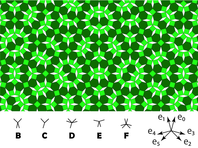
Figure 1: Socolar dodecagonal tiling and five types of vertices. ${\bf e}_{0},{\bf e}_{1},\cdots$, and ${\bf e}_{5}$ are projection of the fundamental translation vectors in six dimensions, ${\bf n}=(1,0,0,0,0,0),(0,1,0,0,0,0),\cdots$, and $(0,0,0,0,0,1)$.

There are some methods to generate the quasiperiodic tilling such as section and strip-projection methods. In our study, we make use of the inflation-deflation rule to generate the lattice Socolar (1989) since it is easy to obtain the exact fractions for various diagrams. The deflation rules for directed hexagons, squares, and rhombuses, are schematically shown in Fig. 2.

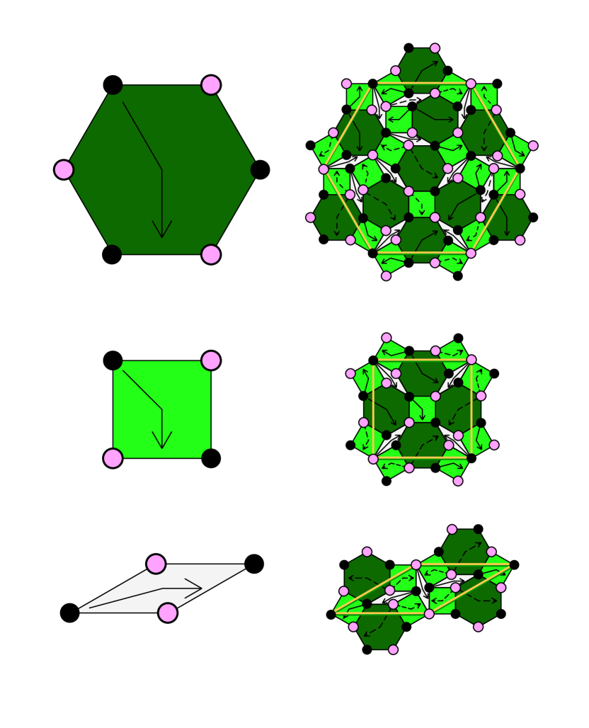
Figure 2: Deflation rule for the dodecagonal tiling Socolar (1989).

It is known that the ratios of the hexagons, squares, and rhombuses are $H:S:R=1:\sqrt{3}:\sqrt{3}$ in the thermodynamic limit Socolar (1989). In the Socolar dodecagonal tiling, there are five kinds of vertices; so-called B, C, D, E, and F vertices (see Fig. 1). We find that, in one deflation process, B, C, D, and E vertices are newly generated in the inside of each hexagon, square, and rhombus, as shown in Fig. 2. On the other hand, the corner sites of the hexagons, squares, and rhombuses are changed into the F vertices under the deflation process. Therefore, we obtain the fractions of the vertices in the thermodynamic limit as

$$p_{B} = \frac{3}{4}\left(5\sqrt{3}-9\right)\sim 0.255,$$ (2)

$$p_{C} = \frac{3}{4}\left(\sqrt{3}-1\right)\sim 0.549,$$ (3)

$$p_{D} = \frac{3}{4}\left(11\sqrt{3}-19\right)\sim 0.0394,$$ (4)

$$p_{E} = \frac{1}{4}\left(9-5\sqrt{3}\right)\sim 0.0849,$$ (5)

$$p_{F} = 7-4\sqrt{3}=\tau^{-2}\sim 0.0718,$$ (6)

where $\tau(=2+\sqrt{3})$ is the ratio characteristic of the dodecagonal tiling.

Next, we consider the sublattice structure in the Socolar dodecagonal tiling since we discuss the magnetically ordered state in the Hubbard model. To this end, we introduce the sublattice-dependent vertices B_σ, C_σ, $\cdots$, F_σ, where $\sigma$ is the sublattice index. Its deflation rule is schematically shown in Fig. 2, where the spin dependence of the vertices is represented by the open and solid circles, and the spin dependence of directed hexagons, squares, and rhombuses are represented by the solid and dashed arrows. Namely, we have defined the spin of one corner vertex, which is located at the root of the arrow, as the spin of the hexagons, squares, and rhombuses. Then, the number of each hexagon, square, and rhombuses at iteration $n$ is changed under the deflation process, which is explicitly given as ${\bf v}_{n+1}=M{\bf v}_{n}$, with ${\bf v}_{n}^{t}=(H_{\uparrow}^{n}\,\,H_{\downarrow}^{n}\,\,S_{\uparrow}^{n}\,\,S_{\downarrow}^{n}\,\,R_{\uparrow}^{n}\,\,R_{\downarrow}^{n})$ and

$$M=\left(\begin{array}[]{cccccc}3&4&1+a&1+a&0&2-2a\\ 4&3&1+a&1+a&2-2a&0\\ 6&6&1+3a&3a&2-3a&4-3a\\ 6&6&3a&1+3a&4-3a&2-3a\\ 6&6&2&2&2&1\\ 6&6&2&2&1&2\end{array}\right),$$ (7)

where $H_{\sigma}^{n}$, $S_{\sigma}^{n}$, and $R_{\sigma}^{n}$ are the number of hexagons, squares, and rhombuses with spin $\sigma$ at the iteration $n$, and $a=2\sqrt{3}/9$. The maximum eigenvalue of the matrix $M$ is $\tau^{2}$, and the corresponding eigenvector is $(1,1,\sqrt{3},\sqrt{3},\sqrt{3},\sqrt{3})^{t}$. Therefore, we can say that no spin imbalance in the hexagons, squares, and rhombuses appears in the thermodynamic limit. As mentioned above, the B, C, D, and E vertices are generated in the inside of the hexagons, squares, and rhombuses in each deflation operation and thereby their fractions do not depend on the spin. Furthermore, F vertices are changed from B, C, D, E, and F vertices in each deflation operation. This concludes no spin dependence in all vertices. Therefore, we can say that the antiferromagnetically ordered state is realized without a net uniform magnetization in the thermodynamic limit Lieb (1989).

When the antiferromagnetically ordered state is considered in the quasiperiodic systems, the density of states in the noninteracting case should play an important role in the weak coupling regime. In fact, the tightbinding model on the Penrose and Ammann-Beenker tilings has a delta function like peak at $E=0$ and the introduction of Coulomb interactions drives the system to the magnetically ordered states with finite magnetizations. Now, we examine the density of states in the tightbinding model on the Socolar dodecagonal tiling. The results for the system with $N=290\,281$ are shown in Fig. 3, where $N$ is the number of site.

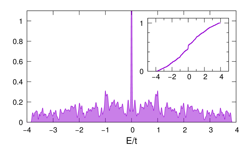
Figure 3: Density of states for the tightbinding model on the Socolar dodecagonal tiling with $N=290\,281$.

Since the vertex model on the Socolar dodecagonal tiling is bipartite, the particle-hole symmetric DOS appears. It is clearly found that the delta function like peak appears at $E=0$, which suggests the existence of the confined states. The fraction of the zero energy states is numerically obtained as $\sim 0.076$. It is known that the value slightly depends on the system size since there are zero energy states around the edge of the system due to the open boundary condition. Nevertheless, in the bulk, there indeed exist the confined states, which is similar to the cases in the Penrose and Ammann-Beenker tilings. In the next section, we examine the confined states in the system in detail.

III Confined states

In the section, we focus on the confined states with $E=0$ in the tightbinding model on the Socolar dodecagonal tiling. Since a wave function described by the linear combination of the confined states is also an eigenstate of the tightbinding Hamiltonian, we can choose the simple state so that its occupied domain is small and has a certain symmetry. Then the domain is represented by a certain point group and the confined state is described by its irreducible representation. Since a certain domain repeats itself in the quasiperiodic tiling, the macroscopically degenerate states are realized in the tightbinding model. This is essentially the same as the Conway’s theorem known in the Penrose tiling. Namely, the fractions of the confined states should be determined exactly.

Table 1: A part of the irreducible characters of the point groups $D_{3}$, $D_{2}$, and $C_{S}$. $E$ is an identity operator, $C_{3}$ is a rotation operator of $2\pi/3$, and $I^{\prime}$ is a reflection operator.

$D_{3}$	$E$	$C_{3}$	$I^{\prime}$
A1	1	1	1
A2	1	1	-1

$D_{2}$	$E$	$C_{2}$	$I_{x}$	$I_{y}$
A	1	1	1	1
B1	1	1	-1	-1
B2	1	-1	1	-1
B3	1	-1	-1	1

$C_{S}$	$E$	$I_{y}$
A1	1	1
A2	1	-1

Now, we focus on the domain in the inside of the Socolar dodecagonal tiling to examine the confined states (see Fig. 1). We find confined states in certain domains represented by the $D_{3}$, $D_{2}$ or $C_{S}$ point group, as shown in Figs. 4, 5, and 6, respectively.

Figure 4: Four confined states in the domains with $D_{3}$ symmetry. The number at the vertices represent the amplitudes of the confined state.

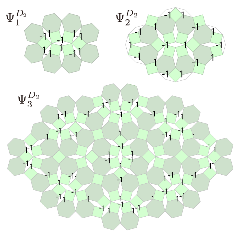
Figure 5: Three confined states in the domains with $D_{2}$ symmetry. The number at the vertices represent the amplitudes of the confined state.

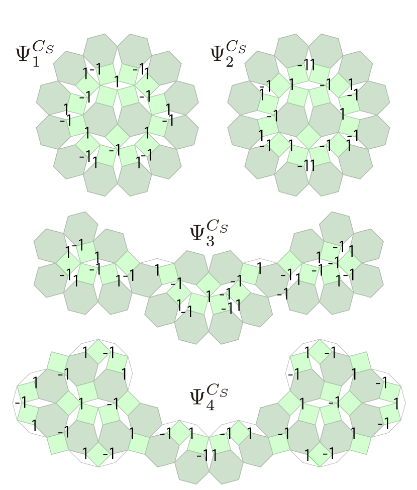
Figure 6: Four confined states in the domains with $C_{S}$ symmetry. The number at the vertices represent the amplitudes of the confined state.

It is also clarified that each confined states should be described by the one-dimensional representation in the corresponding point group, which is explicitly shown in Table 1. The confined state $\Psi_{1}^{D_{3}}$ is described by the representation A₂ in the $D_{3}$ point group, while $\Psi_{2}^{D_{3}}$ is described by A₁, as shown in Fig. 4. We have also found confined states in the larger domains (eg. $\Psi_{3}^{D_{3}}$ and $\Psi_{4}^{D_{3}}$), which can not be described by the linear combinations of the confined states in smaller domains. This should suggest that, in the tightbinding Hamiltonian on the Socolar dodecagonal tiling, there exist infinite kinds of the confined states in larger domains. This is similar to the Ammann-Beenker tiling, while is different from the Penrose tiling. The difference in these confined state properties may be related to the following fact. In the Penrose tiling, due to the existence of the “cluster” structure bounded by “forbidden ladders”, each state is confined only in one cluster and there are no confined states across the forbidden ladders. This should yield a finite gap between the delta-function peak and broad spectrum in the noninteracting density of states Koga and Tsunetsugu (2017). On the other hand, in the Ammann-Beenker and Socolar dodecagonal tilings, there are no “forbidden regions” and therefore the multiple confined states have amplitudes in certain vertices. This should yield energy levels close to the delta function peaks at $E=0$ since the corresponding state should have an amplitude in the whole system. Namely, the gap size $\Delta$ is less than $0.002t$ in the system with $N=290\,281$ (see Fig. 3), which is contrast to the Penrose tiling case with $\Delta\sim 0.17t$ Koga and Tsunetsugu (2017). This should lead to finite magnetization at almost all sites in the Socolar dodecagonal tiling even in the weak coupling limit.

Next, we examine the fraction of each confined state by means of the inflation-deflation rule. First, we consider the confined states described by the $D_{3}$ point group, as shown in Fig. 4. To this end, we consider the region composed of three squares and three rhombuses (${\cal R}_{0}$), which is invariant under $D_{3}$ symmetry operations, as shown in Fig. 7(a). By applying the deflation process to the region ${\cal R}_{0}$, we obtain the larger region ${\cal R}_{1}$, as shown in Fig. 7(b).

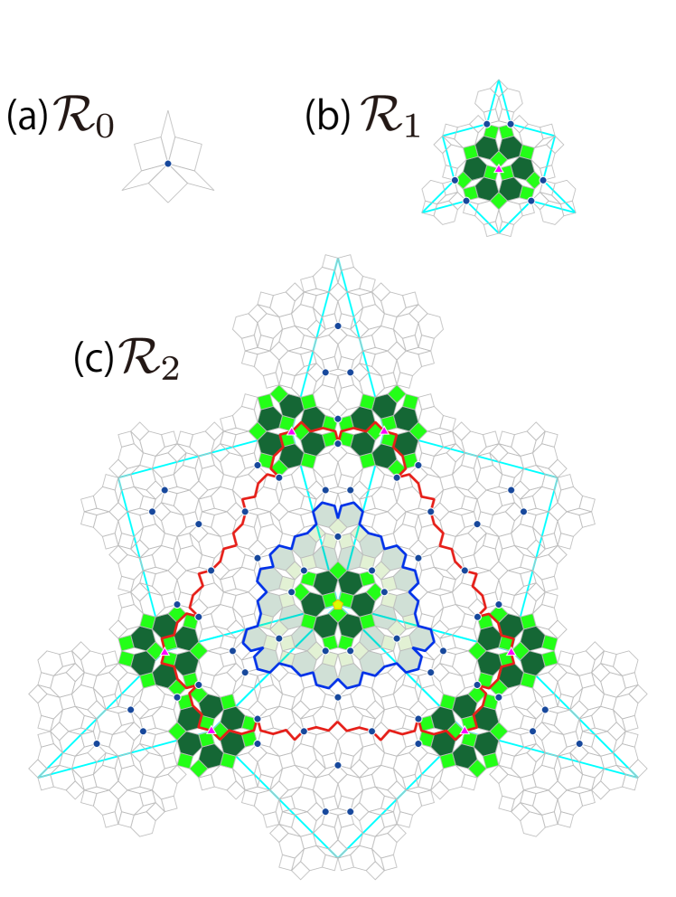
Figure 7: Regions ${\cal R}_{0}$, ${\cal R}_{1}$, and ${\cal R}_{2}$. Circles, triangles, and pentagon represent F₀, F₁, and F₂ vertices. Shaded regions (regions bounded by blue and red lines) represent the domains for $\Psi_{1}^{D_{3}}$ and $\Psi_{2}^{D_{3}}$ $\left(\Psi_{3}^{D_{3}}\right.$ and $\left.\Psi_{4}^{D_{3}}\right)$.

We find that this region includes the structure of the region ${\cal R}_{0}$ around the center and is also invariant under the rotational symmetry. Further application generates the region ${\cal R}_{2}$, as shown in Fig. 7(c). These naturally expect that applying the deflation process to the region ${\cal R}_{i}$, the region ${\cal R}_{i+1}$, in which the structure of ${\cal R}_{i}$ includes, is generated with $D_{3}$ symmetry. Then, one can define the center site of the region ${\cal R}_{i}$ as an F_i vertex, where the integer $i$ strongly depends on the area with local $D_{3}$ symmetry. Namely, in the ${\cal R}_{i}$ region, there should exist F_j vertices away from the center $(j<i)$, which are shown as solid symbols in Fig. 7. The F₀ vertices are newly generated from the B, C, D, E vertices in terms of the deflation operation, and the fraction of the F_i vertices is given as $p_{F_{i}}=(1-\tau^{-2})\tau^{-2i-2}$ in the thermodynamic limit.

Figure 7 shows that there exist the domains for the confined states $\Psi_{1}^{D_{3}}$ and $\Psi_{2}^{D_{3}}$ around the F_i vertices with $i\geq 1$, and the domains for $\Psi_{3}^{D_{3}}$ and $\Psi_{4}^{D_{3}}$ appears around F_i vertices with $i\geq 2$. Therefore, the corresponding fractions are obtained as,

$$p_{1}^{D_{3}} = p_{2}^{D_{3}}=\sum_{i=1}^{\infty}p_{F_{i}}=\frac{1}{\tau^{4}}\sim 0.0052,$$ (8)

$$p_{3}^{D_{3}} = p_{4}^{D_{3}}=\sum_{i=2}^{\infty}p_{F_{i}}=\frac{1}{\tau^{6}}\sim 0.0037.$$ (9)

As for the confined states specified by $D_{2}$ and $C_{S}$ point symmetries, it may be convenient to consider the deflation rule for the hexagons, squares, and rhombuses. Namely, no confined states specified by $D_{2}$ or $C_{S}$ symmetry are obtained by one deflation process (see Fig. 2).

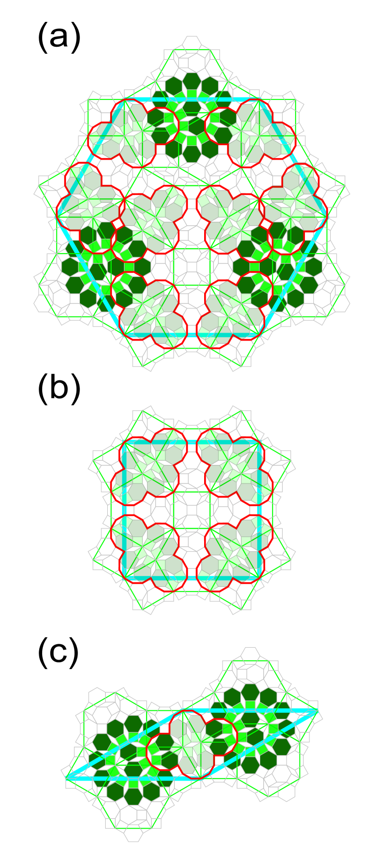
Figure 8: Two deflation processes for (a) hexagon, (b) square, and (c) rhombus. The domains for the confined states $\Psi_{1}^{D_{2}}$ and $\Psi_{1}^{C_{S}}$ are shown as shaded regions.

Figure 8 shows clusters obtained from two deflation processes to one hexagon, square, and rhombus. We find some smallest domains for the confined states $\Psi_{1}^{D_{2}}$ and $\Psi_{2}^{D_{2}}$ ($\Psi_{1}^{C_{S}}$ and $\Psi_{2}^{C_{S}}$). Therefore, the fractions for the confined states are obtained as

$$p_{1}^{D_{2}}=p_{2}^{D_{2}} = \frac{1}{\tau^{4}}\left(8p_{H}+4p_{S}+p_{R}\right)=\frac{1}{\tau^{3}}\sim 0.019,$$ (10)

$$p_{1}^{C_{S}}=p_{2}^{C_{S}} = \frac{1}{\tau^{4}}\left(3p_{H}+2p_{R}\right)=\frac{\tau^{2}+1}{11\tau^{4}}\sim 0.0070,$$ (11)

where the fractions of hexagons, squares, and rhombuses are given as $p_{H}=1/(2\sqrt{3}+1)$ and $p_{S}=p_{R}=\sqrt{3}/(2\sqrt{3}+1)$. The confined states in larger domains, which are shown in Figs. 5 and 6, should appears in the larger regions generated by multiple deflation processes.

In the study, we could find some confined states in smaller domains. Therefore, we can give the lower bound of the fraction of the confined states as,

$$p>p_{lower} = \sum_{i=1}^{4}p_{i}^{D_{3}}+\sum_{i=1}^{2}p_{i}^{D_{2}}+\sum_{i=1}^{2}p_{i}^{C_{S}}$$ (12)

$$= \frac{2}{11\tau^{5}}\left(60\tau+29\right)\sim 0.064.$$ (13)

It is found that the obtained lower bound is consistent with the fraction $0.076$ in the system with $N=290281$. In the following, we clarify how the introduction of the Coulomb interactions realizes the antiferromagnetically ordered states.

IV Effect of the Coulomb interaction

In the section, we consider the Hubbard model with finite $U$. To study the antiferromagnetically ordered state characteristic of the Socolar dodecagonal tiling, we use the real-space Hartree approximation and the Hamiltonian (1) is reduced to

$$H_{MF} = -t\sum_{\langle ij\rangle\sigma}\left(c_{i\sigma}^{\dagger}c_{j\sigma}+h.c.\right)+U\sum_{i\sigma}\langle n_{i\bar{\sigma}}\rangle n_{i\sigma},$$ (14)

where $\langle n_{i\sigma}\rangle$ is the expectation value of the number of electron with spin $\sigma$ at the $i$th site. In our calculations, we deal with finite lattices with $N=72\,274$ and $290\,281$ under the open boundary condition. The lattices are generated by applying the deflation processes to the F vertex. Therefore, the obtained vertex lattices have the global threefold rotational symmetry. For given values of mean-fields, we numerically diagonalize the mean-field Hamiltonian $H_{MF}$ and update the mean-fields, and iterate this selfconsistent procedure until the result converges within numerical accuracy.

We show in Fig. 9 the spatial pattern of the magnetization $m_{i}(=\langle n_{i\uparrow}\rangle-\langle n_{i\downarrow}\rangle)/2$ when $U/t=1.0\times 10^{-7}$, 1, 2, and 5.

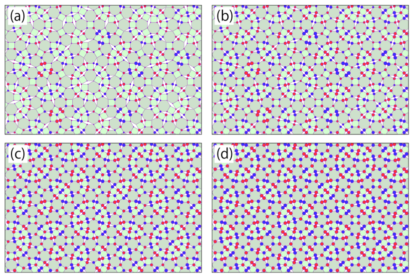
Figure 9: Spatial pattern for the staggered magnetization in the Hubbard model on the Socolar dodecagonal tiling when $U/t=1.0^{-7}$ (essentially the same as $U=0$), 1, 2, and 5. The area of the circles represents the normalized magnitude of the local magnetization.

It is found that finite staggered magnetizations are induced even in the weak coupling limit $U\rightarrow 0$. This originates from the existence of the confined states at $E=0$, as discussed above. In fact, the larger magnetizations appear at the vertices, where the confined states $\Psi_{1}^{D_{2}}$ and $\Psi_{1}^{D_{3}}$ have amplitudes. Increasing the Coulomb interactions, local magnetizations monotonically increase. When $U/t=5$, the staggered magnetizations are almost polarized. It is known that, in the strong coupling case, the system is reduced to the Heisenberg model on the Socolar dodecagonal tiling with nearest neighbor exchanges $J=4t^{2}/U$. The ground state obtained by the mean-field theory is fully polarized with the staggered moment $m_{j}=\pm 1/2$ in the limit. This is different from the results obtained by the spin wave theory for the Heisenberg model, which predicts site-dependent reduction in the spontaneous moments. This reduction originates from intersite quantum fluctuations. Although intersite correlations could not be taken into account in the framework of the mean-field approximations, the essence of crossover behavior in the magnetic properties can be captured correctly.

Finally, we consider the magnetization profile in the perpendicular space. The positions in the perpendicular space have one-to-one correspondence with the positions in the physical space. The vertex sites in the Socolar dodecagonal tiling correspond to a subset of the six-dimensional lattice points $\vec{n}=(n_{0},n_{1},n_{2},n_{3},n_{4},n_{5})$ labeled with integers $n_{m}$ and their coordinates are the projections onto the two-dimensional physical space:

$${\bf r}=(x,y)=\sum_{m=0}^{5}n_{m}{\bf e}_{m},$$ (15)

where ${\bf e}_{m}=(\cos(m\theta+\theta_{0}),\sin(m\theta+\theta_{0}))$ for $m=0,1,4,5$, ${\bf e}_{m}=-(\cos(m\theta+\theta_{0}),\sin(m\theta+\theta_{0}))$ for $m=2,3$, $\theta=2\pi/3$ and the initial phase $\theta_{0}$ is arbitrary, and an example with the choice $\theta_{0}=5\pi/12$. The projection onto the four-dimensional perpendicular space has information specifying the local environment of each site Socolar (1989),

$$\tilde{\bf r} = \sum_{m=0}^{5}n_{m}\tilde{\bf e}_{m},$$ (16)

$${\bf r}^{\perp} = \sum_{m=0}^{5}n_{m}{\bf e}^{\perp}_{m},$$ (17)

where $\tilde{\bf e}_{m}={\bf e}_{5m({\rm mod\,12})}$, ${\bf e}^{\perp}_{m}=(\delta_{m(\rm mod\,2),0},\delta_{m(\rm mod\,2),1})$. ${\bf e}^{\perp}$ takes only four values $(0,0),(0,1),(1,0),(1,1)$, and in each ${\bf e}^{\perp}$ plane the $\tilde{\bf r}$ points densely cover a region with hexagonal shape. The areas and their structures do not depend on planes, which is contrast to the perpendicular space of the Penrose tiling with two distinct planes. Note that the sites with odd and even number of $l={\bf e}^{\perp}\cdot(1,1)$ correspond to the A/B sublattices since upon moving from one site to its neighbor site only one of $n_{m}$’s changes by $\pm 1$. Therefore, the antiferromagnetically ordered state may also be characterized by an alternate sign of the magnetization in the four planes. Then, we can discuss the magnetization profile only in one plane, taking into account the equivalent planes and sign of the magnetization. Figure 10(d) shows one of the planes in the perpendicular space, where each part is the region of the five kinds of vertices. We also find that the F vertices are densely distributed in the hexagonal structure at the center of the perpendicular space. This nested (fractal) structure means that the set of F vertices is the Socolar dodecagonal tiling with larger lattice constant. This is one of the important features characteristic of the Socolar dodecagonal tiling.

The magnetization profile is shown in Fig. 10. In the weak coupling limit, the macroscopically degenerate confined states yield the spatial distribution in the magnetization, which leads to interesting magnetization profile even in the perpendicular space. On the other hand, we could not find the nested structure in the magnetization profile. This is contrast to the magnetic profile in the Hubbard model on the Ammann-Beenker tiling Koga (2020). This may originate from the following. In the Ammann-Beenker tiling case, the confined state located in smaller domains has no amplitudes in the locally symmetric vertices (F vertices), while the confined state has a finite amplitude at the vertices away from the center in the larger domain. The confined states in larger domains have a tiny amplitude in F vertices and their fractions are small, which should lead to the superlattice structure in the magnetic profile. On the other hand, in the Socolar dodecagonal tiling, the confined state $\Psi_{2}^{D_{3}}$ in the smaller domain has an amplitude at the center F vertex, as shown in Fig. 4. Therefore, relatively larger magnetization $|m|\sim 1/26$ is induced although its magnitude should be slightly modified by taking into account the hybridization to other confined states at larger domains.

Increasing $U$, the interesting magnetic pattern smears and magnetic properties become classified by vertices, as shown in Fig. 10. In fact, it seems that, in the perpendicular space, the region of the five kinds of vertices has almost a single staggered magnetization in the system with $U/t=5$, as shown in Fig. 10(c). Then we could find the crossover behavior in the magnetic profile.

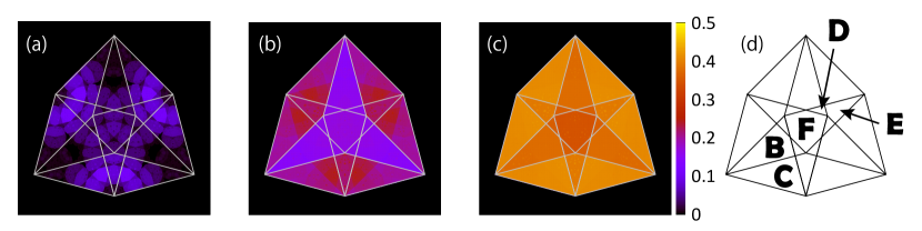
Figure 10: Magnetization profile in the perpendicular space for the system with $N=290\,281$ when $U/t=(a)1.0^{-7}$ (essentially the same as $U=0$), (b) 2, and (c) 5. (d) Each part is the region of the five kinds of vertices shown in Fig. 1.

V Summary

We have studied the antiferromagnetically ordered state in the half-filled Hubbard model on the Socolar dodecagonal tiling. When the interaction is introduced, the staggered magnetizations suddenly appear, which results from the existence of the macroscopically degenerate states in the tightbinding model. By examining the confined states with $E=0$ in detail, we have determined the lower bound of their fraction. The increase of the interaction strength monotonically increases the magnetizations. We have also mapped the spatial distribution of the magnetization to the perpendicular space, and have discussed the magnetization profile. It has been clarified that in the strong coupling regime, the staggered magnetizations are almost classified into five vertices, depending on the site coordination numbers. On the other hand, in the weak coupling regime, the interesting pattern appears in the perpendicular space, which originates from the existence of the confined states.

It has been clarified that the magnetic profile characteristic of the Socolar dodecagonal tiling clearly appears in the real space. Therefore, it may be difficult to observe in the neutron inelastic scattering experiments (the Fourier space). However, we expect that the beautiful magnetic pattern will be observed in the detailed analysis in the spin-dependent scanning tunneling microscopy measurements for the magnetic quasicrystals.