Mostly Harmless Machine Learning:
Learning Optimal Instruments in Linear IV Models

We offer straightforward theoretical results that justify incorporating machine learning in the standard linear instrumental variable setting. The key idea is to use machine learning, combined with sample-splitting, to predict the treatment variable from the instrument and any exogenous covariates, and then use this predicted treatment and the covariates as technical instruments to recover the coefficients in the second-stage. This allows the researcher to extract non-linear co-variation between the treatment and instrument that may dramatically improve estimation precision and robustness by boosting instrument strength. Importantly, we constrain the machine-learned predictions to be linear in the exogenous covariates, thus avoiding spurious identification arising from non-linear relationships between the treatment and the covariates. We show that this approach delivers consistent and asymptotically normal estimates under weak conditions and that it may be adapted to be semiparametrically efficient (Chamberlain, 1992). Our method preserves standard intuitions and interpretations of linear instrumental variable methods, including under weak identification, and provides a simple, user-friendly upgrade to the applied economics toolbox. We illustrate our method with an example in law and criminal justice, examining the causal effect of appellate court reversals on district court sentencing decisions.

1 Introduction

Instrumental variable (IV) designs are a popular method in empirical economics. Over 30% of all NBER working papers and top journal publications considered by Currie et al. (2020) include some discussion of instrumental variables. The vast majority of IV designs used in practice are linear IV estimated via two-stage least squares (TSLS), a familiar technique in standard introductions to econometrics and causal inference (e.g. Angrist and Pischke, 2008). Standard TSLS, however, leaves on the table some variation provided by the instruments that may improve precision of estimates, as it only exploits variation that is linearly related to the endogenous regressors. In the event that the instrument has a low linear correlation with the endogenous variable, but nevertheless predicts the endogenous variable well through a nonlinear transformation, we should expect TSLS to perform poorly in terms of both estimation precision and inference robustness. In particular, in some cases, TSLS would provide spuriously precise but biased estimates (due to weak instruments, see Andrews et al., 2019). Such nonlinear settings become increasingly plausible when exogenous variation includes high dimensional data or alternative data, such as text, images, or other complex attributes like weather. We show that off-the-shelf machine learning techniques provide a general-purpose toolbox for leveraging such complex variation, improving instrument strength and estimate quality.

Replacing the first stage linear regression with more flexible specifications does not come without cost in terms of stronger identifying assumptions. The validity of TSLS hinges only upon the restriction that the instrument is linearly uncorrelated with unobserved disturbances in the response variable. Relaxing the linearity requires that endogenous residuals are mean zero conditional on the exogenous instruments, which is stronger. However, it is rare that a researcher has a compelling reason to believe the weaker non-correlation assumption, but rejects the slightly stronger mean-independence assumption. Indeed, whenever researchers contemplate including higher order polynomials of the instruments, they are implicitly accepting stronger assumptions than TSLS allows. In fact, by not exploiting the nonlinearities, TSLS may accidentally make a strong instrument weak, and deliver spuriously precise inference: Dieterle and Snell (2016) and references therein find that several applied microeconomics papers have conclusions that are sensitive to the specification (linear vs. quadratic) of the first-stage.

A more serious identification concern with leveraging machine learning in the first-stage comes from the parametric functional form in the second stage. When there are exogenous covariates that are included in the parametric structural specification, nonlinear transformations of these covariates could in principle be valid instruments, and provide variation that precisely estimates the parameter of interest. For example, in the standard IV setup of $Y=D^{\top}\tau+X^{\top}\beta+U$ where $X$ is an exogenous covariate, imposing $\mathbb{E}[U\mid X]=0$ would formally result in $X^{2},X^{3}$, etc. being valid “excluded” instruments. However, given that the researcher’s stated source of identification comes from excluded instruments, such “identifying variation” provided by covariates is more of an artifact of parametric specification than any serious information from the data that relates to the researcher’s scientific inquiry.

One principled response to the above concern is to make the second stage structural specification likewise nonparametric, thereby including an infinite dimensional parameter to estimate, making the empirical design a nonparametric instrumental variable (NPIV) design. Significant theoretical and computational progress have been made in this regard (inter alia, Newey and Powell, 2003; Ai and Chen, 2003, 2007; Horowitz and Lee, 2007; Severini and Tripathi, 2012; Ai and Chen, 2012; Hartford et al., 2017; Dikkala et al., 2020; Chen and Pouzo, 2012, 2015; Chernozhukov et al., 2018, 2016). However, regrettably, NPIV has received relatively little attention in applied work in economics, potentially due to theoretical complications, difficulty in interpretation and troubleshooting, and computational scalability. Moreover, in some cases parametric restrictions on structural functions come from theoretical considerations or techniques like log-linearization, where estimated parameters have intuitive theoretical interpretation and policy relevance. In these cases the researcher may have compelling reasons to stick with parametric specifications.

In the spirit of being user-friendly to practitioners, this paper considers estimation and inference in an instrumental variable model where the second stage structural relationship is linear, while allowing for as much nonlinearity in the instrumental variable as possible, without creating unintended and spurious identifying variation from included covariates. Our results provide intuition and justification for using machine learning methods in instrumental variable designs. We show that with sample-splitting, under weak consistency conditions, a simple estimator that uses the predicted values of endogenous and included regressors as technical instruments is consistent, asymptotically normal, and semiparametrically efficient. The constructed instrumental variable also readily provides weak instrument diagnostics and robust procedures. Moreover, standard diagnostics like out-of-sample prediction quality are directly related to quality of estimates. In the presence of exogenous covariates that are parametrically included in the second-stage structural function, adapting machine learning techniques requires caution to avoid spurious identification from functional forms of the included covariates. To that end, we formulate and analyze the problem as a sequential moment restriction, and develop estimators that utilize machine learning for extracting nonlinear variation from and only from instruments.

Related Literature.

The core techniques that allow for the construction of our estimators follow from Chamberlain (1987, 1992). The ideas in our proofs are also familiar in the double machine learning (Chernozhukov et al., 2018; Belloni et al., 2012) and semiparametrics literatures (e.g. Liu et al., 2020); our arguments, however, follow from elementary techniques that are accessible to graduate students and are self-contained. Our proposed estimator is similar to the split-sample IV or jackknife IV estimators in Angrist et al. (1999), but we do not restrict ourselves to linear settings or linear smoothers. Using nonlinear or machine learning in the first stage of IV settings is considered by Xu (2021) (for probit), Hansen and Kozbur (2014) (for ridge), Belloni et al. (2012); Chernozhukov et al. (2015) (for lasso), and Bai and Ng (2010) (for boosting), among others; and our work can be viewed as providing a simple, unified analysis for practitioners, much in the spirit of Chernozhukov et al. (2018). To the best of our knowledge, we are the first to formally explore practical complications of making the first stage nonlinear in a context with exogenous covariates. Finally, we view our work as counterpoint to the recent work by Angrist and Frandsen (2019), which is more pessimistic about combining machine learning with instrumental variables—a point we explore in detail in Section 3.

2 Main theoretical results

We consider the standard cross-sectional setup where the data $(R_{i})_{i=1}^{N}=(Y_{i},D_{i},X_{i},W_{i})_{i=1}^{N}\overset{\mathrm{i.i.d.}}{\sim}P$ are sampled from some infinite population. $Y_{i}$ is some outcome variable, $D_{i}$ is a set of endogenous treatment variables, $X_{i}$ is a set of exogenous controls, and $W_{i}$ is a set of instrumental variables. The researcher is willing to argue that $W_{i}$ is exogenously or quasi-experimentally assigned. Moreover, the researcher believes that $W_{i}$ provides a source of variation that “identifies” an effect $\tau$ of $D_{i}$ on $Y_{i}$. We denote the endogenous variables and covariates as $T_{i}\equiv[1,D_{i}^{\top},X_{i}^{\top}]^{\top}$ and the excluded instrument and covariates as the technical instruments $Z_{i}\equiv[1,W_{i}^{\top},X_{i}^{\top}]^{\top}$.

A typical specification in empirical economics is the linear instrumental variables specification:

$$Y_{i} =\alpha+D_{i}^{\top}\tau+X_{i}^{\top}\beta+U_{i}\quad\mathbb{E}[W_{i}U_{i}]=0.$$ (1)

We believe that often the researcher is willing to assume more than that $U_{i}$ is uncorrelated with $(X_{i},W_{i})$. Common introductions of instrumental variables (Angrist and Pischke, 2008; Angrist and Krueger, 2001) stress that instruments induce variation in $D_{i}$ and are otherwise unrelated to $U_{i}$, and that a common source of instruments is natural experiments. We argue that these narratives imply a stronger form of exogeneity than TSLS requires. After all, a symmetric mean-zero random variable $S$ is uncorrelated with $S^{2}$, but one would be hard pressed to say that $S^{2}$ is unrelated to $S$. Moreover, the condition $\mathbb{E}[W_{i}U_{i}]=0$, strictly speaking, does not automatically make polynomial expansions of $W_{i}$ valid instruments, yet using higher order polynomials is common in empirical research, indicating that the conditional restriction $\mathbb{E}[U_{i}\mid W_{i}]=0$ more accurately captures the assumptions imposed in many empirical projects. With this in mind, we will assume mean independence throughout the paper: $\mathbb{E}[U_{i}\mid W_{i}]=0$. This stronger exogeneity assumption allows researcher to extract more identifying variation from instruments, but doing so calls for more flexible machinery for dealing with the first stage.

2.1 No covariates

Let us first consider the case in which we do not have exogenous covariates $X_{i}$. Our mean-independence restrictions give rise to a conditional moment restriction, $\mathbb{E}[Y_{i}-T_{i}^{\top}\theta\mid W_{i}]=0$, where $\theta=(\alpha,\tau^{\top},\beta^{\top})^{\top}$. The conditional moment restriction encodes an infinite set of unconditional moment restrictions:

$$\text{For all square integrable $\tilde{\upsilon}$}:\mathbb{E}[\tilde{\upsilon}(W_{i})(Y_{i}-T_{i}^{\top}\theta)]=0.$$

Chamberlain (1987) finds that all relevant statistical information in a conditional moment restriction is contained in a single unconditional moment restriction involving an optimal instrument $\Upsilon^{\star}$, and the unconditional moment restriction with the optimal instrument delivers semiparametrically efficient estimation and inference. In our case, $\Upsilon^{\star}(W_{i})=\frac{1}{\sigma^{2}(W_{i})}[1,\mu(W_{i})^{\top}]^{\top}$, where $\mu(W_{i})\equiv\mathbb{E}[D_{i}\mid W_{i}]$ and $\sigma^{2}(W_{i})=\mathbb{E}[U_{i}^{2}\mid W_{i}]$. We estimate $\Upsilon^{\star}$ with $\hat{\Upsilon}$ and form a plug-in estimator for $\theta$:

$$\hat{\theta}_{N}=\left({\frac{1}{N}\sum_{i=1}^{N}\hat{\Upsilon}(W_{i})T_{i}^{\top}}\right)^{-1}\left({\frac{1}{N}\sum_{i=1}^{N}\hat{\Upsilon}(W_{i})Y_{i}}\right).$$ (2)

This is numerically equivalent to estimating (1) with two-stage weighted least-squares with $\hat{\mu}(W_{i})$ as an instrument and weighting with $1/\sigma^{2}(W_{i})$. In particular, if $U_{i}$ is homoskedastic, the optimal instrument is simply $[1,\mu(W_{i})^{\top}]^{\top}$, and two-stage least-squares with an estimate of $\mu(W_{i})$ returns an estimate $\hat{\theta}_{N}$. Under heteroskedasticity, this instrument is no longer optimal (in the sense of semiparametric efficiency) but remains valid. Therefore, we shall refer to the instrument with the weighting $1/\sigma^{2}(W_{i})$ as the optimal instrument under efficient weighting and the instrument without $1/\sigma^{2}(W_{i})$ as the optimal instrument under identity weighting.

Under identity-weighting, estimating $\Upsilon^{\star}$ amounts to learning $\mu(W_{i})\equiv\mathbb{E}[D_{i}\mid W_{i}]$, which is well-suited to machine learning techniques; this is only slightly complicated by the estimation of $\sigma^{2}(W_{i})\equiv\mathbb{E}[U_{i}^{2}\mid W_{i}]$ under efficient weighting. One might worry that the preliminary estimation of $\Upsilon^{\star}$ complicates asymptotic analysis of $\hat{\theta}_{N}$. Under a simple sampling-splitting scheme, however, we state a high-level condition for consistency, normality, and efficiency of $\hat{\theta}_{N}$. Though it simplifies the proof and potentially weakens regularity conditions, sample-splitting does reduce the amount of data used to estimate the optimal instrument $\Upsilon^{\star}$, but such problems can be effectively mitigated by $k$-fold sample-splitting: 20-fold sample-splitting, for instance, limits the loss of data to $5\%$ at the cost of 20 computations that can be effectively parallelized. Such concerns notwithstanding, we focus our exposition to two-fold sample-splitting.

Specifically, assume $N=2n$ for simplicity and let $S_{1},S_{2}\subset[N]$ be the two subsamples with size $n$. Under identity-weighting, for $j\in\{1,2\}$, form $\hat{\Upsilon}^{(j)}$ by estimating $\mu(W_{i})$ with data from the other sample, $S_{-j}$. An estimator for $\mu$ may be a neural network or a random forest trained via empirical risk minimization, or a penalized linear regression such as elastic net. The estimated instrument $\hat{\Upsilon}_{i}$ is then formed by evaluating $\hat{\Upsilon}^{(j)}(W_{i})$ for all $i\in S_{j}$. We may then use (2) to form an (identity-weighted) estimator of $\theta$ by plugging in $\hat{\Upsilon}$. Under efficient weighting, on each $S_{-j}$, we would use the identity-weighted estimator of $\theta$ as an initial estimator to obtain an estimate of $U_{i}$, and similarly predict $U_{i}^{2}$ with $W_{i}$ to form an estimate of $\sigma^{2}(W_{i})$. The resulting estimated optimal instrument under efficient weighting may then be plugged into (2) and form an efficient-weighted estimator. We term such estimators the machine learning split-sample (MLSS) estimators. The pseudocode for major procedures considered in this paper is collected in Algorithm 1.

Theorem 1 shows that the MLSS estimator is consistent and asymptotically normal when the first-stage estimator $\hat{\Upsilon}^{(j)}$ converges to a strong instrument. Moreover, it is semiparametrically efficient when $\hat{\Upsilon}^{(j)}$ is consistent for the optimal instrument $\Upsilon^{\star}(W_{i})\equiv[1,\mu(W_{i})^{\top}]/\sigma^{2}(W_{i})$ in $L^{2}(W)$ norm. The $L^{2}$ consistency condition is not strong—in particular, it is weaker than the $L^{2}$ consistency at $o(N^{-1/4})$-rate conditions commonly required in the double machine learning and semiparametrics literatures (Chernozhukov et al., 2018), where such conditions are considered mild.

Formally, regularity conditions are stated in 1. The first condition simply states that the nuisance estimation attains some limit as sample size tends to infinity, which is a similar requirement as sampling stability in Lei et al. (2018). The second condition states that the limit is a strong instrument. The third condition assumes bounded moments so as to ensure a central limit theorem. The last condition, which is only required for semiparametric efficiency, states that the nuisance estimation is consistent for the optimal instrument in $L^{2}$ norm. For consistency of standard error estimates, we assume more bounded moments in 2.

Assumption 1.

Recall that $Z_{i}=[1,W_{i}^{\top}]$, and so $\Upsilon(W_{i})$ and $\Upsilon(Z_{i})$ denote the same object.

1. ($\hat{\Upsilon}^{(j)}$ attains a limit $\Upsilon$ in $L^{2}$ distance) There exists some measurable function $\Upsilon(Z_{i})$ such that

   $$\mathbb{E}{\lVert\hat{\Upsilon}^{(j)}(Z_{i})-\Upsilon(Z_{i})\rVert^{2}}\to 0\quad\text{ for $j=1,2$,}$$

   where the expectation integrates over both the randomness in $\hat{\Upsilon}^{(j)}$ and in $Z_{i}$, but $\hat{\Upsilon}^{(j)}$ and $Z_{i}$ are assumed to be independent.

2. (Strong identification) The matrix $G\equiv\mathbb{E}[\Upsilon(Z_{i})T_{i}^{\top}]$ exists and is full rank.

3. (Lyapunov condition) (i) For some $\epsilon>0$, the following moments are finite: $\mathbb{E}|U_{i}|^{2+\epsilon}<\infty$, $\mathbb{E}\lVert U_{i}\Upsilon(Z_{i})\rVert^{2+\epsilon}<\infty$, $\mathbb{E}[\lVert T_{i}\rVert^{2}]<\infty$, and (ii) The variance-covariance matrix $\Omega\equiv\mathbb{E}[U_{i}^{2}\Upsilon(Z_{i})\Upsilon(Z_{i})^{\top}]$ exists, and (iii) the conditional variance is uniformly bounded: For some $M$, $\mathbb{E}[U_{i}^{2}\mid Z_{i}]<M<\infty$ a.s.

4. (Consistency to the optimal instrument) We may take the optimal instrument $\Upsilon^{\star}(Z_{i})$ as the limit $\Upsilon(Z_{i})$ in condition 1.

Assumption 2 (Variance estimation).

Let $\Upsilon$ be the object defined in 1. Assume that the following fourth moments are bounded:

$$\max\left\{{\mathbb{E}[\lVert T_{i}\rVert^{4}],\mathbb{E}[U_{i}^{4}],\mathbb{E}\lVert\Upsilon(Z_{i})\rVert^{4},\limsup_{N\to\infty}\mathbb{E}[\lVert\hat{\Upsilon}^{(j)}(Z_{i})\rVert^{4}]}\right\}<\infty.$$

Theorem 1.

Let $\hat{\theta}^{\mathrm{MLSS}}_{N}$ be the MLSS estimator described above. Under conditions 1–3 in 1,

$$\sqrt{N}\left({\hat{\theta}^{\mathrm{MLSS}}_{N}-\theta}\right)\leadsto\mathcal{N}(0,V)\quad\quad V\equiv(G\Omega^{-1}G^{\top})^{-1}=G^{-1}\Omega G^{-\top},$$

where $G,\Omega$ are defined in 1. Moreover, if condition 4 in 1 holds, then the asymptotic variance $V$ attains the semiparametric efficiency bound. Moreover, if we additionally assume 2, then the sample counterparts of $G,\Omega$ are consistent for the two matrices.

Proof of Theorem 1.

We may compute that the scaled estimation error is

$$\sqrt{N}\left({\hat{\theta}^{\mathrm{MLSS}}_{N}-\theta}\right)=\left({\frac{1}{N}\sum_{i=1}^{N}\hat{\Upsilon}(Z_{i})T_{i}^{\top}}\right)^{-1}\frac{1}{\sqrt{N}}\sum_{i=1}^{N}\hat{\Upsilon}(Z_{i})U_{i}.$$

We verify in Lemma 3 that, for $\Upsilon$ defined in condition 1 of 1, the following expansions hold:

$$\hat{G}\equiv\frac{1}{N}\sum_{i=1}^{N}\hat{\Upsilon}(Z_{i})T_{i}^{\top}=\frac{1}{N}\sum_{i=1}^{N}\Upsilon(Z_{i})T_{i}^{\top}+o_{p}(1)\qquad\frac{1}{\sqrt{N}}\sum_{i=1}^{N}\hat{\Upsilon}(Z_{i})U_{i}=\frac{1}{\sqrt{N}}\sum_{i=1}^{N}\Upsilon(Z_{i})U_{i}+o_{p}(1).$$ (3)

Expansion (3) implies that $\hat{\theta}^{\mathrm{MLSS}}_{N}$ is first-order equivalent to the oracle estimator that plugs in $\Upsilon$:

$$\hat{\theta}^{\star}_{N}\equiv\left({\frac{1}{N}\sum_{i=1}^{N}\Upsilon(Z_{i})T_{i}^{\top}}\right)^{-1}\frac{1}{N}\sum_{i=1}^{N}\Upsilon(Z_{i})Y_{i},$$

whose consistency and asymptotic normality follows from usual arguments under condition 3 of 1. Given (3), then we have a law of large numbers $\frac{1}{N}\sum_{i=1}^{N}\hat{\Upsilon}(Z_{i})T_{i}^{\top}\overset{p}{\longrightarrow}G$ by condition 2 of 1; and we obtain a central limit theorem $\frac{1}{\sqrt{N}}\sum_{i=1}^{N}\Upsilon(Z_{i})U_{i}\leadsto\mathcal{N}(0,\Omega)$ by condition 3. Lastly, by Slutsky’s theorem and the fact that $G$ is nonsingular, we obtain the desired convergence $\smash{\sqrt{N}\left({\hat{\theta}^{\mathrm{MLSS}}_{N}-\theta}\right)\leadsto\mathcal{N}(0,V)}$.

If, additionally, we assume the consistency condition 4, then $\hat{\theta}^{\star}_{N}$ is exactly the efficient optimal instrument estimator (Chamberlain, 1987), and hence $V$ attains the semiparametric efficiency bound. Finally, (3) implies that $\hat{G}\overset{p}{\longrightarrow}G$ via a weak law of large numbers, and Lemma 4 implies $\hat{\Omega}\equiv\frac{1}{N}\sum_{i=1}^{N}(Y_{i}-T_{i}^{\top}\hat{\theta}^{\mathrm{MLSS}}_{N})^{2}\hat{\Upsilon}_{i}\hat{\Upsilon}_{i}^{\top}\overset{p}{\longrightarrow}\Omega$, and thus the variance can be consistently estimated. ∎

2.2 Exogenous covariates

The presence of covariates $X_{i}$ complicates the analysis considerably. Under the researcher’s model, both $W_{i}$ and $X_{i}$ are considered exogenous, and thus we may assume $\mathbb{E}[U_{i}\mid Z_{i}]=0$ and use it as a conditional moment restriction, under which the efficient instrument is $\operatorname{Var}(U_{i}\mid Z_{i})^{-1}\mathbb{E}[T_{i}\mid Z_{i}]$ and our analysis from the previous section continues to apply mutatis mutandis. However, if the researcher maintains a linear specification $Y_{i}=T_{i}^{\top}\theta+U_{i}$, estimating $\theta$ based on the conditional moment restriction $\mathbb{E}[U_{i}\mid Z_{i}]=0$ may inadvertently “identify” $\theta$ through nonlinear behavior in $X_{i}$ rather than the variation in $W_{i}$. Such a specification may allow the researcher to precisely estimate $\theta$ even when the instrument $W_{i}$ is completely irrelevant, when, say, higher-order polynomial terms in the scalar $X_{i}$, $X_{i}^{2},X_{i}^{3}$, are strongly correlated with $D_{i}$, perhaps due to misspecification of the linear moment condition. There may well be compelling reasons why these nonlinear terms in $X_{i}$ allow for identification of $\tau$ under an economic or causal model; however, they are likely not the researcher’s stated source of identification, and allowing their influence to leak into the estimation procedure undermines credibility of the statistical exercise.

One idea to resolve such a conundrum is to make the structural function nonparametric as well, and convert the model to a nonparametric instrumental variable regression (Newey and Powell, 2003; Ai and Chen, 2003, 2007, 2012; Chen and Pouzo, 2012) (See Appendix B for discussion). Another idea, which we undertake in this paper, is to weaken the moment condition and rule nonlinearities in $X_{i}$ as inadmissible for inference.

To that end, we analyze the statistical restrictions implied by the model and consider relaxations. The conditional moment restriction $\mathbb{E}[U_{i}\mid Z_{i}]=0$ is equivalent to the following orthgonality constraint

$$\text{For all (square integrable) $\Upsilon$},\,\mathbb{E}[\Upsilon(W_{i},X_{i})(Y_{i}-T_{i}^{\top}\theta)]=0.$$ (4)

Condition (4) is too strong, since it allows nonlinear transforms of $X_{i}$ to be valid instruments. A natural idea is to restrict the class of allowable instruments $\Upsilon(W_{i},X_{i})$ to those that are partially linear in $X_{i}$, $\Upsilon(W_{i},X_{i})=h(W_{i})+X_{i}^{\top}\ell$, thereby deliberately discarding information from nonlinear transformations of $X_{i}$. Doing so yields the following family of orthogonality constraints:

$$\text{For all (square integrable) $\Upsilon$},\,\mathbb{E}[\Upsilon(W_{i})(Y_{i}-T_{i}^{\top}\theta)]=\mathbb{E}[X_{i}(Y_{i}-T_{i}^{\top}\theta)]=0.$$ (5)

We may view (5) as imposing an orthogonality condition on the structural errors $U_{i}$ that is intermediate between that of TSLS and that of (4). In particular, if we define $\mathbb{E}_{\mathrm{(PL)}}[\cdot\mid X_{i},W_{i}]$ as a projection operator that projects onto partially linear functions of $(X_{i},W_{i})$:

$$\mathbb{E}_{\mathrm{(PL)}}[U_{i}\mid X_{i},W_{i}]\equiv\operatorname*{arg\,min}_{\begin{subarray}{c}h(X_{i},W_{i})\\ h(X_{i},W_{i})=X_{i}^{\top}\ell+g(W_{i})\end{subarray}}\mathbb{E}\left({U_{i}-h(X_{i},W_{i})}\right)^{2},$$

then requiring (5) is equivalent to requiring orthogonality under this partially linear projection operator:

$$\mathbb{E}_{\mathrm{(PL)}}[U_{i}\mid X_{i},W_{i}]=0.$$ (6)

In contrast, the $\operatorname{Cov}(U_{i},Z_{i})=0$ orthogonality requirement of TSLS can be written as $\mathbb{E}_{\mathrm{(L)}}[\cdot\mid Z_{i}]=0$, where $\mathbb{E}_{\mathrm{(L)}}[\cdot\mid Z_{i}]$ is analogously defined as a projection operator onto linear functions of $Z_{i}$. We see that (6) is a natural interpolation between the respective orthogonality structures on the errors $U_{i}$ induced by the TSLS and the conditional moment restrictions.

The moment restriction corresponding to (5) is the following sequential moment restriction

$$\mathbb{E}[X_{i}(Y_{i}-T_{i}^{\top}\theta)]=\mathbb{E}[Y_{i}-T_{i}^{\top}\theta\mid W_{i}]=0.$$ (7)

We see that (7) is a natural interpolation between the usual unconditional moment condition, $\mathbb{E}[Z_{i}U_{i}]=0$, and the conditional moment restriction that may be spurious $\mathbb{E}[U_{i}\mid Z_{i}]=0$, by only allowing nonlinear information in $W_{i}$ to be used for estimation and inference.

Having set up the estimation problem as (equivalently) characterized by (5), (6), or (7), efficient estimation is discussed by Chamberlain (1992). In particular, the optimal instrument under identity weighting takes the convenient form

$$\Upsilon^{\star}(Z_{i})=\mathbb{E}_{\mathrm{(PL)}}\left[{T_{i}\mid X_{i},W_{i}}\right]=\begin{bmatrix}1\\ \mathbb{E}_{\mathrm{(PL)}}\left[{D_{i}\mid X_{i},W_{i}}\right]\\ X_{i}\end{bmatrix},$$ (8)

which is simply $(1,X_{i})$, along with the best partially linear prediction of the endogenous treatment $D_{i}$ from $W_{i},X_{i}$. Observe that the only difference between (8) and Chamberlain (1987)’s optimal instrument under homoskedasticity is modifying $\mathbb{E}$ into $\mathbb{E}_{\mathrm{(PL)}}$. Implementing (8) is straightforward, as by Robinson (1988), partially linear regression is reducible to fitting two nonparametric regressions $\mathbb{E}[D_{i}\mid W_{i}]$ and $\mathbb{E}[X_{i}\mid W_{i}]$, and forming the following prediction function

$$\mathbb{E}_{\mathrm{(PL)}}\left[{D_{i}\mid X_{i},W_{i}}\right]=\mathbb{E}[D_{i}\mid W_{i}]+\mathbb{E}_{\mathrm{(L)}}[D_{i}\mid\left({X_{i}-\mathbb{E}[X_{i}\mid W_{i}]}\right)].$$

Table 1: List of nonparametric nuisance parameters that require estimation. Note that nuisance parameters that require the unobserved error $U_{i}$ require additional preliminary consistent estimators of $\theta$.

Covariates $X_{i}$	Identity weighting?	Nonparametric nuisance parameters
No	Yes	$\mathbb{E}[D_{i}\mid W_{i}]$
No	No	$\mathbb{E}[D_{i}\mid W_{i}]$, $\mathbb{E}[U_{i}^{2}\mid W_{i}]$
Yes	Yes	$\mathbb{E}[D_{i}\mid W_{i}]$, $\mathbb{E}[X_{i}\mid W_{i}]$
Yes	No	$\mathbb{E}[D_{i}\mid W_{i}]$, $\mathbb{E}[X_{i}U_{i}^{2}\mid W_{i}]$, $\mathbb{E}[U_{i}^{2}\mid W_{i}]$

Efficient estimation in the heteroskedastic case is more complex. The optimal instrument is the vector

$$\Upsilon^{\star}(Z_{i})=\frac{\mathbb{E}[T_{i}\mid W_{i}]}{\sigma^{2}(W_{i})}+\mathbb{E}\left[{T_{i}\tilde{X}_{i}^{\top}}\right]\mathbb{E}\left[{U_{i}^{2}\tilde{X}_{i}\tilde{X}_{i}^{\top}}\right]^{-1}\tilde{X}_{i},\quad\tilde{X}_{i}\equiv X_{i}-\frac{\mathbb{E}[X_{i}U_{i}^{2}\mid W_{i}]}{\sigma^{2}(W_{i})}$$

and the associated set of unconditional moment restrictions are

$$\mathbb{E}\left[{U_{i}\cdot\Upsilon^{\star}(Z_{i})}\right]=0.$$ (9)

The intuition for (9) is the following: the two moment conditions $\mathbb{E}[U_{i}X_{i}]=\mathbb{E}[U_{i}\mid W_{i}]=0$ provide non-orthogonal information for $\theta$ that prevents us from applying the optimal instrument on each moment condition. However, we may orthogonalize one against the other. In particular, the moment condition $\mathbb{E}[\tilde{X}_{i}U_{i}]=0$ is orthogonal to $\mathbb{E}[U_{i}\mid W_{i}]$ in the sense that $\mathbb{E}[\tilde{X}_{i}U_{i}\cdot U_{i}\mid W_{i}]=0$. Indeed, the term $\frac{\mathbb{E}[X_{i}U_{i}^{2}\mid W_{i}]}{\sigma^{2}(W_{i})}U_{i}\equiv\frac{\langle X_{i}U_{i},U_{i}\rangle}{\langle U_{i},U_{i}\rangle}U_{i}$ is constructed to be the projection of $X_{i}U_{i}$ onto $U_{i}$ under the inner product $\langle A,B\rangle=\mathbb{E}[AB\mid W_{i}]$.

As before, complications in nonparametric estimation can be avoided by sample splitting, where nuisance parameters are estimated on $K-1$ folds of the data and the moment condition is evaluated on the remaining fold. As a summary across our settings, we collect the nuisance parameters that require a first-step estimation in Table 1. The estimator

$$\hat{\theta}^{\mathrm{MLSS}}_{N}=\left({\frac{1}{N}\sum_{i=1}^{N}\hat{\Upsilon}(Z_{i})T_{i}^{\top}}\right)^{-1}\frac{1}{N}\sum_{i=1}^{N}\hat{\Upsilon}(Z_{i})Y_{i}$$

remains the same as (2) and is subjected to the same analysis in Theorem 1—under conditions 1–3 in 1, $\hat{\theta}^{\mathrm{MLSS}}_{N}$ is consistent and asymptotically normal, and additionally, it is semiparametrically efficient if the $L^{2}$-limit of $\hat{\Upsilon}$ coincides with the optimal instrument $\Upsilon^{\star}$ in their respective settings.

Lastly, we make two remarks about the case with exogenous covariates, assuming identity weighting for tractability. First, it is possible for $\mathbb{E}[D_{i}\mid W_{i}]=0$ and for (8) to generate precise estimates of the coefficient $\tau$. The reason is that it is possible for the partially linear specification $D_{i}=h(W_{i})+X_{i}^{\top}\ell+V_{i}$ to generate nonzero $h(W_{i})$ but zero conditional expectation, in much the same way that some regression coefficients may be zero without adjusting for $X_{i}$, but nonzero when adjusted for $X_{i}$. Whether or not this makes $W_{i}$ a plausibly exogenous and strong instrument is likely to be context specific. A robustness check may be generated by replacing $\mathbb{E}_{\mathrm{(PL)}}[D_{i}\mid X_{i},W_{i}]$ with $\mathbb{E}[D_{i}\mid W_{i}]$, which delivers consistent and asymptotically normal estimates (assuming strong instrument) at the cost of efficiency. Second, a Frisch-Waugh-Lovell- or double machine learning-like procedure of first partialling out $X_{i}$ from $Y_{i},D_{i}$ and then treating

$$Y_{i}-\mathbb{E}_{\mathrm{(L)}}[Y_{i}\mid X_{i}]=\tau\left({D_{i}-\mathbb{E}_{\mathrm{(L)}}[D_{i}\mid X_{i}]}\right)+U_{i}\quad\mathbb{E}[U_{i}\mid W_{i}]=0$$ (10)

as a conditional moment restriction also delivers consistent and asymptotically normal estimates. However, using the “optimal” instrument for (10)—the predicted residual $\mathbb{E}[D_{i}-\mathbb{E}_{\mathrm{(L)}}[D_{i}\mid X_{i}]\mid W_{i}]$—does not achieve semiparametric efficiency, since it uses the information in the sequential moment restriction (7) separately, without considering them jointly and orthogonalizing one against the other, resulting in efficiency loss.

Algorithm 1 Machine learning split-sample estimation and inference

A subroutine PredictInstrument($S_{-j},S_{j}$) that returns the estimated instrument $\{\hat{\Upsilon}(Z_{i}):i\in S_{j}\}$, where $\hat{\Upsilon}$ is a function of $S_{-j}$.

procedure GenerateInstrument($K$, Data)

     Randomly split data into $S_{1},\ldots,S_{K}$

     for $j$ in 1,…, $K$ do

         $\hat{\Upsilon}^{(j)}\leftarrow\mathrm{PredictInstrument}(S_{-j},S_{j})$

     end for

     Combine $\hat{\Upsilon}^{(j)}$ into $\hat{\Upsilon}$

     Return $S_{1},\ldots,S_{K},\hat{\Upsilon}$

end procedure

procedure MLSSEstimate($K$, Data)

     $S_{1},\ldots,S_{K},\hat{\Upsilon}\leftarrow\mathrm{GenerateInstrument}(K,\mathrm{Data})$

     For the full parameter vector, return

$$\hat{\theta}=\left({\frac{1}{N}\sum_{i=1}^{N}\hat{\Upsilon}(W_{i})T_{i}^{\top}}\right)^{-1}\left({\frac{1}{N}\sum_{i=1}^{N}\hat{\Upsilon}(W_{i})Y_{i}}\right)$$

and variance estimate

$$\hat{V}=\left({\frac{1}{N}\sum_{i=1}^{N}\hat{\Upsilon}_{i}T_{i}^{\top}}\right)\cdot\left({\frac{1}{N}\sum_{i=1}^{N}(Y_{i}-T_{i}^{\top}\hat{\theta})^{2}\hat{\Upsilon}_{i}\hat{\Upsilon}_{i}^{\top}}\right)\cdot\left({\frac{1}{N}\sum_{i=1}^{N}\hat{\Upsilon}_{i}T_{i}^{\top}}\right)^{-\top}$$

     For the subvector $\hat{\tau}$, residualize $\hat{\Upsilon}_{i},Y_{i},D_{i}$ against $X_{i}$ to obtain $\tilde{\upsilon}_{i},\tilde{Y}_{i},\tilde{D}_{i}$, and compute $\hat{\tau}=\left({\frac{1}{N}\sum_{i=1}^{N}\tilde{\upsilon}_{i}\tilde{D}_{i}^{\top}}\right)^{-1}\left({\frac{1}{N}\sum_{i=1}^{N}\tilde{\upsilon}_{i}\tilde{Y}_{i}}\right).$ $\triangleright$ Assuming identity weighting

end procedure

procedure WeakIVInference($K$, Data, $\alpha$) $\triangleright$ Assuming identity weighting $\triangleright$ Assuming a routine AndersonRubin($\alpha,\mathrm{Data}$) that returns the $1-\alpha$ Anderson–Rubin CI

     $S_{1},\ldots,S_{K},\hat{\Upsilon}\leftarrow\mathrm{GenerateInstrument}(K,\mathrm{Data})$

     for $j$ in 1,…, $K$ do

         On $S_{j}$, residualize $\hat{\Upsilon}^{(j)}(Z_{i}),Y_{i},D_{i}$ against $X_{i}$ to obtain $\tilde{\upsilon}_{i},\tilde{Y}_{i},\tilde{D}_{i}$

         $\mathrm{CI}_{j}\leftarrow\mathrm{AndersonRubin}\left({\alpha/K,\left\{{\tilde{\upsilon}_{i},\tilde{Y}_{i},\tilde{D}_{i}}\right\}_{i\in S_{j}}}\right)$

     end for

     Return $\mathrm{CI}=\bigcap_{j}\mathrm{CI}_{j}$

end procedure

3 Discussion

“Forbidden regression.” Nonlinearities in the first stage are often discouraged due to a “forbidden regression,” where the researcher regresses $Y$ on $\hat{D}$ estimated via nonlinear methods, motivated by a heuristic explanation for TSLS. As Angrist and Krueger (2001) point out, this regression is inconsistent, and consistent estimation follows from using $\hat{D}$ as an instrument for $D$, as we do, rather than replacing $D$ with $\hat{D}$—in the case where the first-stage is linear, the two estimates are numerically equivalent, but not in general.

Interpretation under heterogeneous treatment effects.

Assume $D_{i}$ is binary and suppose $Y_{i}=D_{i}Y_{i}(1)+(1-D_{i})Y_{i}(0)$. Suppose the treatment follows a Roy model, $D_{i}=\mathbbm{1}\left({\mu(W_{i})\geq V_{i}}\right)$, where $V_{i}\sim\operatorname{Unif}[0,1]$. In this setting, the conditional moment restriction (1) is misspecified, since it assumes constant treatment effects, and different choices of the instrument would generate estimators that converge to different population quantities. Nevertheless, the results of Heckman and Vytlacil (2005) (Section 4) show that different choices of the instrument generate estimators that estimate different weightings of marginal treatment effects (MTEs); moreover, optimal instruments, whether under identity weighting or optimal weighting, correspond to convex averages of MTEs, whereas no such guarantees are available for linear IV estimators with $W_{i}$ as the instrument, without assuming that $\mathbb{E}[D_{i}\mid W_{i}]$ is linear. The weights on the MTEs are explicitly stated in Appendix D.

Weak IV detection and robust inference.

A major practical motivation for our work, following Bai and Ng (2010), is to use machine learning to rescue otherwise weak instruments due to a lack of linear correlation; nonetheless, the instrument may be irredeemably weak, and providing weak-instrument robust inference is important in practice. Relatedly, Xu (2021) and Antoine and Lavergne (2019) also consider weak IV inference with nonlinear first-stages; the benefits of split-sampling in the presence of many or weak instruments are recently exploited by Mikusheva and Sun (2020) and date to Dufour (2003), Angrist et al. (1999), Staiger and Stock (1994), and references therein; Kaji (2019) proposes a general theory of weak identification in semiparametric settings.

On weak IV detection, our procedure produces estimated optimal instruments, which result in just-identified moment conditions. As a result, in models with a single endogenous treatment variable, the Stock and Yogo (2005) $F$-statistic rule-of-thumb has its exact interpretation regardless of homo- or heteroskedasticity (Andrews et al., 2019), and the first stage $F$-statistic may be used as a tool for detecting weak instruments.

Pre-testing for weak instruments distorts downstream inferences. Alternatively, weak IV robust inferences, which are inferences of $\tau$ that are valid regardless of instrument strength, are often preferred. The procedure we propose, under identity-weighting, is readily compatible with simple robust procedures. In particular, on each subsample $S_{j}$, we may perform the Anderson–Rubin test (Anderson et al., 1949) and combining the results across subsamples via Bonferroni correction. For a confidence interval at the 95% nominal level with two-fold sample-splitting, this amounts to intersecting two 97.5%-nominal AR confidence intervals on each subsample, and these confidence intervals may be computed using off-the-shelf software implementations of AR confidence intervals.

More formally, consider the null hypothesis $H_{0}:\tau=\tau_{0}$. Consider a Frisch–Waugh–Lovell procedure that partials out the covariates $X_{i}$. Let the residuals be $U_{i}(\tau_{0})\equiv Y_{i}-D_{i}^{\top}\tau_{0}$, and let $\tilde{U}_{i}(\tau_{0})\equiv U_{i}(\tau_{0})-\tilde{\delta}^{\top}\overline{X}_{i}$ be the residual $U_{i}(\tau_{0})$ after partialling out $\overline{X}_{i}\equiv[1,X_{i}^{\top}]^{\top}$. Suppose the estimated instrument takes the form $\hat{\Upsilon}(Z_{i})=[1,\hat{\upsilon}(Z_{i})^{\top},X_{i}^{\top}]^{\top}$, where $\dim\hat{\upsilon}(Z_{i})=\dim D_{i}$; this requirement is satisfied under identity weighting. Similarly, partial out $\overline{X}_{i}$ from the estimated instrument to obtain $\tilde{\upsilon}^{(j)}\equiv\hat{\upsilon}^{(j)}-\tilde{\lambda}^{\top}\overline{X}_{i}$. Finally, consider the covariance $V_{n,j}(\tau_{0})$ between the residual and the instrument, after partialling out the covariates $\overline{X}_{i}$, and let $\Omega_{n,j}$ be an estimate of $V_{n,j}$’s variance matrix: i.e.,

$$V_{n,j}(\tau_{0})\equiv\frac{1}{\sqrt{n}}\sum_{i\in S_{j}}\hat{\upsilon}^{(j)}(Z_{i})\tilde{U}_{i}(\tau_{0})\text{ and }\Omega_{n,j}(\tau_{0})\equiv\frac{1}{n}\sum_{i\in S_{j}}\tilde{U}_{i}(\tau_{0})^{2}\tilde{\upsilon}^{(j)}(Z_{i})\tilde{\upsilon}^{(j)}(Z_{i})^{\top}.$$

The Anderson–Rubin statistic on the $j$-th subsample is then defined as the normalized magnitude of $V_{n,j}$: $\operatorname{AR}_{j}(\tau_{0})\equiv V_{n,j}^{\top}\Omega_{n,j}^{-1}V_{n,j}.$ Under $H_{0}$, by virtue of the exclusion restriction, we should expect $V_{n,j}$ be mean-zero Gaussian, and thus $\operatorname{AR}_{j}$ should be $\chi^{2}$. Indeed, Theorem 2 shows that on each subsample, under mild bounded moment conditions that ensure convergence (3), $\operatorname{AR}_{j}(\tau_{0})$ attains a limiting $\chi^{2}$ distribution. Under weak IV asymptotics, it is not necessarily the case that the AR statistics are asymptotically uncorrelated across subsamples, and so we resort to the Bonferroni procedure in outputting a single confidence interval.

Assumption 3 (Bounded moments for the AR statistic).

Without loss of generality and normalizing if necessary, assume the estimated instruments are normalized: $\sum_{i\in S_{j}}\hat{\upsilon}^{(j)}_{k}(Z_{i})^{2}=1$ for all $k=1,\ldots,\dim D_{i}$. Let $\lambda_{n}\equiv\mathbb{E}[\overline{X}_{i}\overline{X}_{i}]^{-1}\mathbb{E}[\hat{\upsilon}^{(j)}(Z_{i})\overline{X}_{i}^{\top}\mid\hat{\upsilon}^{(j)}]$ be the projection coefficient of $\hat{\upsilon}^{(j)}(Z_{i})$ onto $\overline{X}_{i}$. Assume that with probability 1, the sequence $\hat{\upsilon}^{(j)}=\hat{\upsilon}^{(j)}_{n}$ satisfies the Lyapunov conditions

1. $\mathbb{E}[U_{i}^{4}\lVert\hat{\upsilon}^{(j)}(Z_{i})-\lambda_{n}\overline{X}_{i}\rVert^{4}\mid\hat{\upsilon}^{(j)}]<C_{1}<\infty$ for some $C_{1}>0$

2. $\mathbb{E}[U_{i}^{2}(\hat{\upsilon}^{(j)}(Z_{i})-\lambda_{n}\overline{X}_{i})(\hat{\upsilon}^{(j)}(Z_{i})-\lambda_{n}\overline{X}_{i})^{\top}\mid\hat{\upsilon}^{(j)}]\overset{p}{\longrightarrow}\Omega$.

Moreover, assume (iii) $\max\left\{{\mathbb{E}[\lVert\hat{\upsilon}^{(j)}\rVert^{4}],\mathbb{E}[U_{i}^{4}],\mathbb{E}[\lVert X_{i}\rVert^{4}]}\right\}<C_{2}<\infty$ and that (iv) $\mathbb{E}[\overline{X}_{i}\overline{X}_{i}^{\top}]$ is invertible.

Theorem 2.

Under 3, $\operatorname{AR}_{j}(\tau_{0})\leadsto\chi^{2}_{\dim D_{i}}$.

Proof.

We relegate the proof, which amounts to checking convergences $V_{n,j}\leadsto\mathcal{N}(0,\Omega)$ and $\Omega_{n,j}\overset{p}{\longrightarrow}\Omega$ under 3, to the appendix. ∎

Connection between first-stage fitting and estimate quality.

By using machine learning in the first stage, one may be able to improve the quality of the first-stage fit, as measured by out-of-sample $R^{2}$. We now offer an argument as to why improving that fit may improve the mean squared error of the estimator.

Consider a setting with no covariates and i.i.d. $U_{i}$ and an estimated instrument $\hat{\upsilon}(Z_{i})$, meant to approximate $\mathbb{E}[D_{i}\mid Z_{i}]$. In linear IV, $\hat{\upsilon}(Z_{i})$ is the linear projection of $D_{i}$ onto $Z_{i}$. Define the extra-sample error of an estimator $\hat{\tau}$ based on $\hat{\upsilon}(Z_{i})$ to be the random quantity

$$\mathrm{Err}(\hat{\upsilon}) \equiv{n\cdot\left({\frac{\operatorname{Cov}_{n}(\hat{\upsilon}(Z_{i}),Y_{i})}{\operatorname{Cov}_{n}(\hat{\upsilon}(Z_{i}),D_{i})}-\tau}\right)^{2}}$$

where $(Y_{i},D_{i},Z_{i})_{i=1}^{n}$ is a new and independent sample unrelated to the estimate $\hat{\upsilon}$, and we hold $\hat{\upsilon}$ fixed. The subscript $n$ denotes sample quantities such as sample variances and covariances. The quantity $\mathrm{Err}(\hat{\upsilon})$ is an optimistic measure of the quality of using $\hat{\upsilon}$ as the instrument, as construction of $\hat{\upsilon}$ without sample-splitting typically introduces a bias term since $\operatorname{Cov}(\hat{\upsilon},U_{i})$ cannot be assumed to be small. The following calculation shows that $\mathrm{Err}(\hat{\upsilon})$ scales with the inverse out-of-sample $R^{2}$ of $\hat{\upsilon}$ as a predictor of $D_{i}$:

$$\mathrm{Err}(\hat{\upsilon}) ={n\frac{\operatorname{Cov}_{n}(\hat{\upsilon}(Z_{i}),U_{i})^{2}}{\operatorname{Cov}_{n}(\hat{\upsilon}(Z_{i}),D_{i})^{2}}}$$

$$={\frac{1}{R^{2}_{n}\left({\hat{\upsilon}(Z_{i}),D_{i}}\right)}\cdot\operatorname{Var}_{n}(D_{i})^{-1}\left({\frac{1}{\sqrt{n}}\sum_{i=1}^{n}\frac{\hat{\upsilon}(Z_{i})}{\sqrt{\operatorname{Var}_{n}(\hat{\upsilon}(Z_{i}))}}(U_{i}-\overline{U})}\right)^{2}}$$

$$\leadsto\frac{1}{R^{2}\left({\hat{\upsilon}(Z_{i}),D_{i}}\right)}\frac{\operatorname{Var}(U_{i})}{\operatorname{Var}(D_{i})}\cdot\chi^{2}_{1}\quad\text{as $n\to\infty$},$$

where $R^{2}_{n}$ is the out-of-sample $R^{2}$ of predicting $D_{i}$ with $\hat{\upsilon}(Z_{i})$, and $R^{2}(\cdot,\cdot)$ is its limit in probability.

The out-of-sample $R^{2}$, which can be readily computed from a split-sample procedure, therefore offers a useful indicator for quality of estimation. In particular, if one is comfortable with the strengthened identification assumptions, there is little reason not to use the model that achieves the best out-of-sample prediction performance on the split-sample. In some settings, this best-performing model will be linear regression, but in many settings it may not be, and attempting more complex tools may deliver considerable benefits.

Moreover, much of the discussion on using machine learning for instrumental variables analysis focuses on selecting (relevant or valid) instruments (Belloni et al., 2012; Angrist and Frandsen, 2019) assuming some level of sparsity, motivated by statistical difficulties encountered when the number of instruments is high. In light of the heuristic above, a more precise framing is perhaps combining instruments to form a better prediction of the endogenous regressor, as noted by Hansen and Kozbur (2014).

(When) is machine learning useful?

We conclude this section by discussing our work relative to Angrist and Frandsen (2019), who note that using lasso and random forest methods in the first stage does not seem to provide large performance benefits in practice, on a simulation design based on the data of Angrist and Krueger (1991). We note that, per our discussion above in the connection between first-stage fitting and estimate quality, a good heuristic summary for the estimation precision is the $R^{2}$ between the fitted instrument and the true optimal instrument—$\mathbb{E}[D_{i}\mid W_{i}]$ in the homoskedastic case. It is quite possible that in some settings, the conditional expectation $\mathbb{E}[D_{i}\mid W_{i}]$ is estimated well with linear regression, and lasso or random forest do not provide large benefits in terms of out-of-sample prediction quality. Since Angrist and Krueger (1991)’s instruments are quarter-of-birth interactions and are hence binary, it is in fact likely that predicting $D$ with linear regression performs well relative to nonlinear or complex methods in the setting. Whether or not machine learning methods work well relative to linear methods is something that the researcher may verify in practice, via evaluating performance on a hold-out set, which is standard machine learning practice but is not yet widely adopted in empirical economics. Indeed, we observe that in both real (Section 4) and Monte Carlo (Appendix C) settings where the out-of-sample prediction quality of more complex machine learning methods out-perform linear regression, MLSS estimators perform better than TSLS.

4 Empirical Application

We consider an empirical application in the criminal justice setting of Ash et al. (2019), where we consider the causal effect of appellate court decisions at the U.S. circuit court level on lengths of criminal sentences at the U.S. district courts under the jurisdiction of the circuit court. Ash et al. (2019) exploit the fact that appellate judges are randomly assigned, and use the characteristics of appellate judges—including age, party affiliation, education, and career backgrounds—as instrumental variables. In criminal justice cases, plaintiffs rarely appeal, as it would involve trying the defendant twice for the same offense—generally not permitted in the United States; therefore, an appellate court reversal would typically be in favor of defendants, and we may posit a causal channel in which such reversals affect sentencing; for instance, the district court may be more lenient as a result of a reversal, as would be naturally predicted if the reversal sets up a precedent in favor of the defendant.

To connect the empirical setting with our notation, the outcome variable $Y$ is the change in sentencing length before and after an appellate decision, measured in months, where positive values of $Y$ indicates that sentences become longer after the appellate court decision. The endogenous treatment variable $D$ is whether or not an appellate decision reverses a district court ruling. The instruments $W$ are the characteristics of the randomly assigned circuit judge presiding over the appellate case in question, and covariates $X$ contain textual features from the circuit case, represented by Doc2Vec embeddings (Le and Mikolov, 2014).

We compute two estimators of the optimal instrument under identity weighting based on flexible methods that are often characterized as machine learning (random forest and LightGBM, for light gradient boosting machine), as well as a variety of linear or polynomial regression estimators, with or without sample-splitting. We present our results in Figure 1 (see the notes to the figure for precise definitions of each estimator). For all of the split-sample estimators we have three sets of point estimates and confidence intervals, corresponding to the different splits. We also have specifications that exclude (panel (a)) and include covariates (panel (b)); except where discussed below the results are consistent across both.

The machine learning estimators perform similarly across splits, reporting mildly negative point estimates of between $1$ and $2$ months reduction in sentencing, with confidence intervals that are reasonably tight but include a zero effect. Moreover, the Wald and Anderson–Rubin confidence intervals are similar, suggesting that the instrument constructed by the ML methods is sufficiently strong to result in inferences that are not distorted.

A natural benchmark to compare these results to is TSLS, with the instruments entering either linearly or quadratically (but not interacted). Linear TSLS estimates a slightly positive effect without covariates and a slightly negative one with them. Though it has a tight Wald confidence interval, the AR interval is quite large ($[-3.3,23.8]$). This indicates a weak instruments problem, and indeed the first-stage $F$-statistic is only 1.5. Quadratic TSLS returns a point estimate that is close to the MLSS estimates, with a very tight Wald confidence interval; however, the corresponding Anderson–Rubin interval is empty. Anderson–Rubin tests test model misspecification jointly with point nulls of the structural coefficient, and may report an empty interval if the model is misspecified. Moreover, we should still be concerned with weak instruments: The first-stage $F$-statistic is only $2.2$ (excluding covariates) and $2.3$ (including covariates).

The sample-splitting estimators based on traditional polynomial expansions rather than machine learning all perform poorly, with out-of-sample $R^{2}$ close to zero and consequently huge confidence intervals (the point estimates also vary wildly across splits). Overall, the MLSS estimators successfully extract more variation from the instruments than the alternatives, and consequently deliver more statistical precision.

(a) Excluding covariates

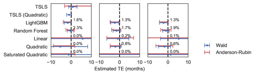
(b) Including covariates

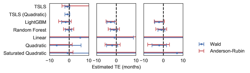
Notes: Point estimate and confidence intervals across three sample splits, represented by the three horizontal panels. TSLS and TSLS (Quadratic) are direct estimates without sample-splitting. Out-of-sample $R^{2}$ of instruments on endogenous treatment in annotation in panel (a).

TSLS is a standard TSLS estimator without sample splitting, using the instruments directly from the dataset. TSLS (Quadratic) includes second-order terms (but not interactions) for the instruments, again without sample-splitting—in particular, it results in an empty Anderson–Rubin interval. LightGBM and RandomForest are MLSS estimators, where LightGBM is an algorithm for gradient boosted trees. Finally, Linear, Quadratic, and Saturated Quadratic are split-sample estimators with linear regression, quadratic regression (without interactions), and quadratic regression with interactions as the estimators for the instrument, respectively.

Figure 1: IV estimation of the effect of appellate court reversal on district court sentencing decisions

5 Conclusion

In this paper, we provide a simple and user-friendly analysis of incorporating flexible prediction into instrumental variable analysis in a manner that is familiar to applied researchers. In particular, we document via elementary techniques that a split-sample IV estimator with machine learning methods as the first stage inherits classical asymptotic and optimality properties of usual instrumental regression, requiring only weak conditions governing the consistency of the first stage prediction. In the presence of covariates, we also formalize moment conditions for instrumental regression that continues to leverage nonlinearities in the excluded instrument without creating spurious identification from the nonlinearities in the included covariates. Leveraging such nonlinearity in the first stage allows the user to extract more identifying variation from the instrumental variables and can have the potential of rescuing seemingly weak instruments into strong ones, as we demonstrate with simulated data and real data from a criminal justice context. Conventional components of an instrumental variable analysis, such as identification-robust confidence sets, extend seamlessly in the presence of a machine learning first stage. We believe that machine learning in IV settings is a mostly harmless addition to the empiricist’s toolbox.

Appendix A Technical lemmas and proofs

Lemma 3.

Under conditions 1 and 3 of 1, we have (3).

Proof.

We first consider the first statement. Observe that

$$\frac{1}{N}\sum_{i=1}^{N}\left({\hat{\Upsilon}(Z_{i})-\Upsilon(Z_{i})}\right)T_{i}^{\top}=\frac{1}{2}\sum_{j\in\{1,2\}}\frac{1}{n}\sum_{i\in S_{j}}\left({\hat{\Upsilon}^{(j)}(Z_{i})-\Upsilon(Z_{i})}\right)T_{i}^{\top}$$

We control the right-hand side, where $\lVert\cdot\rVert_{F}$ is the Frobenius norm:

$$\bigg{\lVert}\frac{1}{n}\sum_{i\in S_{j}}\left({\hat{\Upsilon}^{(j)}(Z_{i})-\Upsilon(Z_{i})}\right)T_{i}^{\top}\bigg{\rVert}_{F}^{2} \leq\left({\frac{1}{n}\sum_{i\in S_{j}}\lVert\hat{\Upsilon}^{(j)}(Z_{i})-\Upsilon(Z_{i})\rVert\cdot\lVert T_{i}\rVert}\right)^{2} \lVert AB\rVert_{F}\leq\lVert A\rVert_{F}\lVert B\rVert_{F}$$ ()

$$\leq\left({\frac{1}{n}\sum_{i\in S_{j}}\lVert\hat{\Upsilon}^{(j)}(Z_{i})-\Upsilon(Z_{i})\rVert^{2}}\right)\left({\frac{1}{n}\sum_{i\in S_{j}}\lVert T_{i}\rVert^{2}}\right)$$ (Cauchy–Schwarz)

$$=O_{p}(1)\frac{1}{n}\sum_{i\in S_{j}}\lVert\hat{\Upsilon}^{(j)}(Z_{i})-\Upsilon(Z_{i})\rVert^{2} \mathbb{E}\lVert T_{i}^{2}\rVert<\infty$$ (Since in condition 3)

$$\overset{p}{\longrightarrow}0$$

The last step follows, because the nonnegative random variable $n^{-1}\sum_{i\in S_{j}}\lVert\hat{\Upsilon}^{(j)}(Z_{i})-\Upsilon(Z_{i})\rVert^{2}\geq 0$ has expectation converging to zero by condition 1 of 1. Therefore

$$\frac{1}{N}\sum_{i=1}^{N}\left({\hat{\Upsilon}(Z_{i})-\Upsilon(Z_{i})}\right)T_{i}^{\top}=\frac{1}{2}\sum_{j\in\{1,2\}}\frac{1}{n}\sum_{i\in S_{j}}\left({\hat{\Upsilon}^{(j)}(Z_{i})-\Upsilon(Z_{i})}\right)T_{i}^{\top}=o_{p}(1).$$

We now consider the second statement. Again we may decompose

$$\frac{1}{N}\sum_{i=1}^{N}\left({\hat{\Upsilon}(Z_{i})-\Upsilon(Z_{i})}\right)U_{i}=\frac{1}{2}\sum_{j\in\{1,2\}}\frac{1}{n}\sum_{i\in S_{j}}\left({\hat{\Upsilon}^{(j)}(Z_{i})-\Upsilon(Z_{i})}\right)U_{i}\equiv\frac{Q_{1}+Q_{2}}{2}$$

and show that $\sqrt{n}Q_{j}\equiv\sqrt{n}\frac{1}{n}\sum_{i\in S_{j}}\left({\hat{\Upsilon}^{(j)}(Z_{i})-\Upsilon(Z_{i})}\right)U_{i}\equiv\sqrt{n}\frac{1}{n}\sum_{i\in S_{j}}\Delta_{i}U_{i}=o_{p}(1),$ where we write $\hat{\Upsilon}^{(j)}(Z_{i})-\Upsilon(Z_{i})=\Delta_{i}$ as a shorthand.

It suffices to show that $\operatorname{Var}\left({Q_{j}}\right)=o(1)$, since $Q_{j}=\mathbb{E}Q_{j}+O_{p}(\sqrt{\operatorname{Var}(Q_{j})})$ and $\mathbb{E}[Q_{j}]=0$. Note that

$$\operatorname{Var}(Q_{j})=\frac{1}{n}\sum_{i}\mathbb{E}[\Delta^{2}_{i}\cdot\mathbb{E}[U_{i}^{2}\mid S_{-j},Z_{i}]]\leq\frac{1}{n}\sum_{i}\mathbb{E}[\Delta_{i}^{2}]\cdot M$$ (Condition 3, 1)

which vanishes. ∎

Lemma 4.

Under 2 and condition 3 of 1, $\hat{\Omega}\equiv\frac{1}{N}\sum_{i=1}^{N}(Y_{i}-T_{i}^{\top}\hat{\theta}^{\mathrm{MLSS}}_{N})^{2}\hat{\Upsilon}_{i}\hat{\Upsilon}_{i}^{\top}\overset{p}{\longrightarrow}\Omega$.

Proof.

Observe that $(Y_{i}-T_{i}^{\top}\hat{\theta}^{\mathrm{MLSS}}_{N})^{2}=U_{i}^{2}+(\theta-\hat{\theta}^{\mathrm{MLSS}}_{N})^{\top}(T_{i}T_{i}^{\top}(\theta-\hat{\theta}^{\mathrm{MLSS}}_{N})+2U_{i}T_{i})\equiv U_{i}^{2}+(\theta-\hat{\theta}^{\mathrm{MLSS}}_{N})^{\top}V_{i}$, where we define $V_{i}=T_{i}T_{i}^{\top}(\theta-\hat{\theta}^{\mathrm{MLSS}}_{N})+2U_{i}T_{i}$ . Note that

$$\bigg{\lVert}(\theta-\hat{\theta}^{\mathrm{MLSS}}_{N})^{\top}\frac{1}{N}\sum_{i=1}^{N}V_{i}\hat{\Upsilon}_{i}\hat{\Upsilon}_{i}^{\top}\bigg{\rVert}_{F} \leq\lVert\theta-\hat{\theta}^{\mathrm{MLSS}}_{N}\rVert\cdot\frac{1}{N}\sum_{i=1}^{N}\lVert V_{i}\rVert\lVert\hat{\Upsilon}_{i}\rVert^{2}$$

$$\leq o_{p}(1)\left({\frac{1}{N}\sum_{i=1}^{N}V_{i}^{2}\cdot\frac{1}{N}\sum_{i=1}^{N}\lVert\hat{\Upsilon}_{i}\rVert^{4}}\right)^{1/2}$$

$\frac{1}{N}\sum_{i=1}^{N}\lVert V_{i}\rVert^{2}$ is $O_{p}(1)$ if $\lVert T_{i}\rVert^{4},\lVert U_{i}\rVert^{4}$ have bounded expectations. $\frac{1}{N}\sum_{i=1}^{N}\lVert\hat{\Upsilon}_{i}\rVert^{4}$ is $O_{p}(1)$ since $\Upsilon$ has bounded fourth moments and so does the difference $\lVert\hat{\Upsilon}-\Upsilon\rVert$. Thus

$$\hat{\Omega}=\frac{1}{N}\sum_{i=1}^{N}U_{i}^{2}\hat{\Upsilon}_{i}\hat{\Upsilon}_{i}^{\top}+o_{p}(1).$$

Next, we may compute

$$\bigg{\lVert}\frac{1}{N}\sum_{i=1}^{N}(\hat{\Upsilon}_{i}\hat{\Upsilon}_{i}^{\top}-\Upsilon_{i}\Upsilon_{i}^{\top})U_{i}^{2}\bigg{\rVert}_{F}\leq\frac{1}{N}\sum_{i=1}^{N}2U_{i}^{2}\lVert\Upsilon_{i}\rVert\lVert\hat{\Upsilon}_{i}-\Upsilon_{i}\rVert+\frac{1}{N}\sum_{i=1}^{N}\lVert\hat{\Upsilon}_{i}-\Upsilon_{i}\rVert^{2}U_{i}^{2}.$$

Note that the expectation of the second term on the right-hand side vanishes:

$$\mathbb{E}[\lVert\hat{\Upsilon}_{i}-\Upsilon_{i}\rVert^{2}\mathbb{E}[U_{i}^{2}\mid S_{-j},Z_{i}]]\leq M\mathbb{E}[\lVert\hat{\Upsilon}_{i}-\Upsilon_{i}\rVert^{2}]\to 0.$$

Thus the second term is a nonnegative sequence with vanishing expectation, and is hence $o_{p}(1)$. To show that the first term is $o_{p}(1)$, it suffices to show that

$$\mathbb{E}[U_{i}^{2}\lVert\Upsilon_{i}\rVert\lVert\hat{\Upsilon}_{i}-\Upsilon_{i}\rVert]=o_{p}(1).$$

This is in turn true since, by condition 3 of 1 and Cauchy–Schwarz

$$\mathbb{E}[U_{i}^{2}\lVert\Upsilon_{i}\rVert\lVert\hat{\Upsilon}_{i}-\Upsilon_{i}\rVert]<M\cdot\sqrt{\mathbb{E}[\lVert\Upsilon_{i}\rVert^{2}]\mathbb{E}[\lVert\hat{\Upsilon}_{i}-\Upsilon_{i}\rVert^{2}]}=o_{p}(1).\qed$$

Theorem 5 (Theorem 2 in the main text).

Under 3, $\operatorname{AR}_{j}(\tau_{0})\leadsto\chi^{2}_{\dim D_{i}}$.

Proof.

We first show that $V_{n,j}\leadsto\mathcal{N}(0,\Omega)$. Observe that $\tilde{U}_{i}=-(\tilde{\delta}-\delta)^{\top}\overline{X}_{i}+U_{i}$ where

$$(\tilde{\delta}-\delta)=\left[{\frac{1}{n}\sum_{i}\overline{X}_{i}\overline{X}_{i}^{\top}}\right]^{-1}\frac{1}{n}\sum_{i}\overline{X}_{i}U_{i}^{\top}.$$

Then

$$V_{n,j} =\frac{1}{\sqrt{n}}\sum_{i\in S_{j}}\hat{\upsilon}^{(j)}(Z_{i})U_{i}-\left({\frac{1}{\sqrt{n}}\sum_{i\in S_{j}}\hat{\upsilon}^{(j)}(Z_{i})\overline{X}_{i}^{\top}}\right)(\tilde{\delta}-\delta)$$

$$=\frac{1}{\sqrt{n}}\sum_{i\in S_{j}}\hat{\upsilon}^{(j)}(Z_{i})U_{i}-\left({\frac{1}{n}\sum_{i\in S_{j}}\hat{\upsilon}^{(j)}(Z_{i})\overline{X}_{i}^{\top}}\right)\sqrt{n}(\tilde{\delta}-\delta)$$

$$=\frac{1}{\sqrt{n}}\sum_{i\in S_{j}}\left({\hat{\upsilon}^{(j)}(Z_{i})-\lambda_{n}^{\top}\overline{X}_{i}}\right)U_{i}+o_{p}(1).$$

The last equality follows from expanding $(\tilde{\delta}-\delta)$ and applying the following laws of large numbers (in triangular arrays):

$$\frac{1}{n}\sum_{i}\overline{X}_{i}\overline{X}_{i}^{\top}=\underbrace{\mathbb{E}[\overline{X}_{i}\overline{X}_{i}]}_{\text{invertible}}+o_{p}(1)\quad\frac{1}{n}\sum_{i}\hat{\upsilon}^{(j)}(Z_{i})\overline{X}_{i}^{\top}=\mathbb{E}[\hat{\upsilon}^{(j)}(Z_{i})X_{i}^{\top}\mid\hat{\upsilon}^{(j)}]+o_{p}(1),$$

for which the fourth-moment conditions (iii), (iv) of 3 are sufficient. The conditions (i) and (ii) are then Lyapunov conditions for the central limit theorem $V_{n,j}\leadsto\mathcal{N}(0,\Omega)$ conditional on $\hat{\upsilon}^{(j)}$. Since the limiting distribution does not depend on $\hat{\upsilon}^{(j)}$ and the conditions are stated as $\hat{\upsilon}^{(j)}$-almost-sure, $V_{n,j}\leadsto\mathcal{N}(0,\Omega)$ unconditionally as well.

Next, we show that $\Omega_{n,j}\overset{p}{\longrightarrow}\Omega$. By condition (ii) and law of large numbers (so that $\frac{1}{n}\sum_{i}U_{i}^{2}(\hat{\upsilon}^{(j)}(Z_{i})-\lambda_{n}\overline{X}_{i})(\hat{\upsilon}^{(j)}(Z_{i})-\lambda_{n}\overline{X}_{i})^{\top}\overset{p}{\longrightarrow}\Omega$), it suffices to show that

$$\Omega_{n,j}=\frac{1}{n}\sum_{i}U_{i}^{2}(\hat{\upsilon}^{(j)}(Z_{i})-\lambda_{n}\overline{X}_{i})(\hat{\upsilon}^{(j)}(Z_{i})-\lambda_{n}\overline{X}_{i})^{\top}+o_{p}(1).$$

Write $\tilde{U}_{i}=U_{i}-(\tilde{\delta}-\delta)^{\top}\overline{X}_{i}$ and $\tilde{\upsilon}^{(j)}=[\hat{\upsilon}^{(j)}-\lambda_{n}\overline{X}_{i}]-(\tilde{\lambda}-\lambda_{n})^{\top}\overline{X}_{i}$. Expanding the sum yields

$$\Omega_{n,j}=\frac{1}{n}\sum_{i}U_{i}^{2}[\hat{\upsilon}^{(j)}-\lambda_{n}\overline{X}_{i}][\hat{\upsilon}^{(j)}-\lambda_{n}\overline{X}_{i}]^{\top}+(\tilde{\delta}-\delta)^{\top}\left({\frac{1}{n}\sum_{i}A_{in}}\right)+(\tilde{\lambda}-\lambda_{n})^{\top}\left({\frac{1}{n}\sum_{i}B_{in}}\right)$$

for some $A_{in},B_{in}$ that involve products of up to four terms of $U_{i},\overline{X}_{i},\hat{\upsilon}^{(j)}$. Since the fourth moments are bounded by (iii), we have that $\frac{1}{n}\sum_{i}A_{in}=O_{p}(1)$ and $\frac{1}{n}\sum_{i}B_{in}=O_{p}(1)$. Since $\tilde{\delta}-\delta$ and $\tilde{\lambda}-\lambda_{n}$ are both $o_{p}(1)$, we have the desired expansion. Therefore, by Slutsky’s theorem, $\operatorname{AR}_{j}(\tau)\leadsto Z^{\top}\Omega^{-1}Z\sim\chi^{2}_{\dim D_{i}}$ where $Z\sim\mathcal{N}(0,\Omega)$. ∎

Appendix B Discussion related to NPIV

A principled modeling approach is the NPIV model, which treats the unknown structural function $g$ as an infinite dimensional parameter and considers the model

$$\mathbb{E}[Y-g(T)\mid Z]=0.$$

The researcher may be interested in $g$ itself, or some functionals of $g$, such as the average derivative $\theta=\mathbb{E}\left[{\frac{\partial{g}}{\partial{D}}(T)\mid Z}\right]$ or the best linear approximation $\beta=\mathbb{E}[TT^{\top}]^{-1}\mathbb{E}[Tg(T)].$ One might wonder whether choosing a parametric functional form in place of $g(T)$ is without loss of generality. Linear regression of $Y$ on $T$, for instance, yields the best linear approximation to the structural function $\mathbb{E}[Y|T]$, and thus has an attractive nonparametric interpretation; it may be tempting to ask whether an analogous property holds for IV regression. If an analogous property does hold, we may have license in being more blasé about linearity in the second stage.

Unfortunately, modeling $g$ as linear does not produce the best linear approximation, at least not with respect to the $L^{2}$-norm. Escanciano and Li (2020) show that the best linear approximation can be written as a particular IV regression estimand

$$\beta=\mathbb{E}[h(Z)T^{\top}]^{-1}\mathbb{E}[h(Z)Y]$$

where $h$ has the property that $\mathbb{E}[h(Z)|T]=T$. Note that with efficient instrument in a homoskedastic, no-covariate linear IV context as we consider in Section 2.1, the optimal instrument is $\hat{D}(W)=\mathbb{E}[D|W]$. A sufficient condition, under which the IV estimand based on the optimal instrument is equal to the best linear approximation $\beta$, is the somewhat strange condition that the projection onto $D$ of predicted $D$ is linear in $D$ itself: For some invertible $A$, $\mathbb{E}[\hat{D}(W)|D]=AD.$ The condition would hold, for instance, in a setting where $D,W$ are jointly Gaussian and all conditional expectations are linear, but it is difficult to think it holds in general. As such, linear IV would not recover the best linear approximation to the nonlinear structural function in general.

A simple calculation can nevertheless characterize the bias of the linear approach if we take the estimand to be the best linear approximation to the structural function. Suppose we form an instrumental variable estimator that converges to an estimand of the form

$$\gamma=\mathbb{E}[f(Z)T^{\top}]^{-1}\mathbb{E}[f(Z)Y].$$

It is easy to see that

$$\gamma-\beta=\langle g-\mathbb{E}^{*}[g|T],\mu-\mathbb{E}^{*}[\mu|T]\rangle,$$

where $\langle A,B\rangle=\mathbb{E}[AB]$, $\mu(T)=\mathbb{E}[f(Z)|T]$, and $\mathbb{E}^{*}[A|B]$ is the best linear projection of $A$ onto $B$. This means that the two estimands are identical if and only if at least one of $\mu(\cdot)$ or $g(\cdot)$ are linear, and all else equal the bias is smaller if $\mu$ or $g$ is more linear. Importantly, $\mu-\mathbb{E}^{*}[\mu|T]$ are objects that we could empirically estimate since they are conditional means, and in practice the researcher may estimate $\mu-\mathbb{E}^{*}[\mu|T]$, which delivers bounds on $\gamma-\beta$ through assumptions on linearity of $g$.

Appendix C Monte Carlo example

C.1 Without covariates

We consider a Monte Carlo experiment where there are three instruments $W_{0},W_{1},W_{2}\overset{\mathrm{i.i.d.}}{\sim}\mathcal{N}(0,1)$, one binary treatment variable $D$, and an outcome $Y$. The probability of treatment is a nonlinear function of the instruments

$$\operatorname{Pr}(D=1\mid W)=\sigma(3\mu(W_{0},W_{1}))\sin(2W_{2})^{2}\quad\sigma(t)=\frac{1}{1+e^{-t}}$$

where

$$\mu(W_{0},W_{1})=\begin{cases}0.1&W_{0}^{2}+W_{1}^{2}>1\\ \operatorname{sgn}(W_{0}W_{1})(W_{0}^{2}+W_{1}^{2})&\text{otherwise}\end{cases}$$

Naturally, the choice of $\mu$ implies an XOR-function-like pattern in the propensity of getting treated, where $D=1$ is more likely when $W_{0},W_{1}$ is the same sign, and less likely when $W_{0},W_{1}$ is of different signs. An empirical illustration of the joint distribution of $D,W_{0},W_{1}$ is in Figure 2.

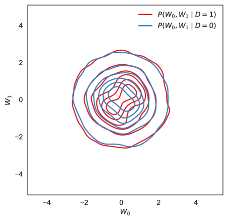
Figure 2: Conditional density of the first two instruments $W_{0},W_{1}$ given treatment status

The outcome $Y$ is generated by $Y=D+v(W_{0},W_{1},W_{2})U$, where

$$U=0.5(D-\operatorname{Pr}(D=1\mid W))|Z_{1}|+\sqrt{1-0.5^{2}}Z_{2}$$

where $Z_{1},Z_{2}\sim\mathcal{N}(0,1)$ independently, and $v(W_{0},W_{1},W_{2})=0.1+\sigma((W_{0}+W_{1})W_{2}).$ Importantly, by construction, $\mathbb{E}[U\mid W]=0$, and the true treatment effect is $\tau=1$.

We consider a variety of estimators for the first stage $\mathbb{E}[D\mid W]$ in a split-sample IV estimation routine. In particular, we consider two machine learning estimators (LightGBM and random forest) versus a variety of more classical linear regression estimators based on taking transformations (polynomial or discretization) of $W_{0},W_{1},W_{2}$ and estimating via OLS on the transformed instruments. For the traditional, linear regression-based estimators, we also consider TSLS without sample splitting. The performances of the estimators, as well as their definitions, are summarized in Figure 3.

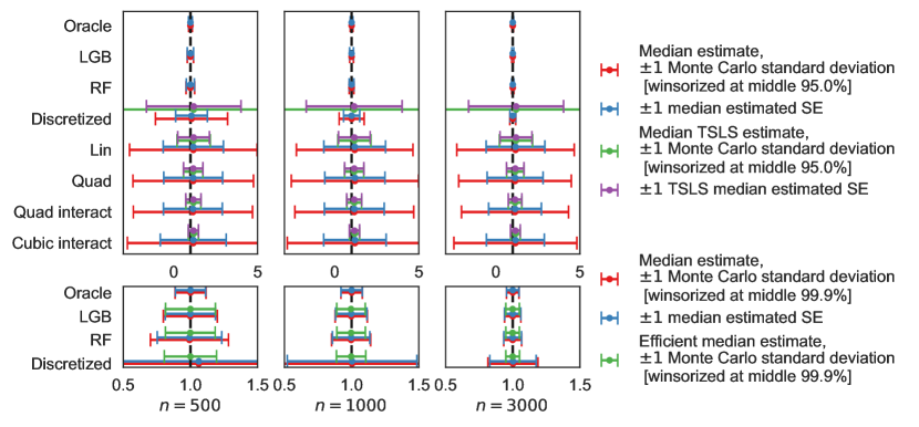
Notes: Median estimates, winsorized standard deviation, and median estimated standard error reported for a variety of estimators. The Monte Carlo standard deviations are computed from winsorized point estimates since the finite-sample variance of the linear IV estimator may not exist.

The estimators are split-sample IV estimators that differ in their construction of the instrument: Oracle refers to using the true form $\operatorname{Pr}(D=1\mid W)$ as the instrument; LGB refers to using LightGBM, a gradient boosting algorithm; RF refers to using random forest; Discretized refers to discretizing $W_{0},W_{1},W_{2}$ into four levels at thresholds $-1,0,1$, and using all $4^{3}$ interactions as categorical covariates; Lin refers to linear regression with $W_{0},W_{1},W_{2}$ untransformed; Quad refers to quadratic regression without interactions; Quad interact refers to quadratic regression with full interactions; and Cubic interact refers to cubic regression with full interactions.

The latter five estimators (Discretized through Cubic interact) may also be implemented directly with TSLS without sample splitting, and we also plot the corresponding performance summaries in the top panel (in green and purple).

The bottom panel is a zoomed-in version of the best performing estimators. We also show the performance of the efficient estimator (estimating the optimal instrument with inverse-variance weighting) in the bottom panel in green.

Figure 3: Performance of a variety of estimators for $\tau$ in the setting of Section C.1

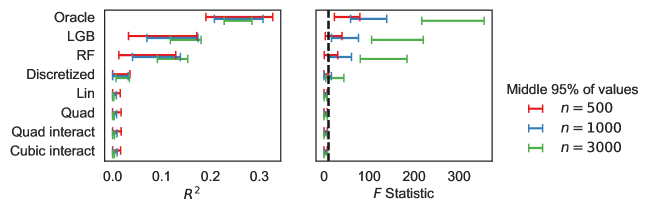
Figure 4: Fit statistics of a variety of estimators for $\tau$ in the setting of Section C.1. The dashed line reports the Stock and Yogo (2005) rule of thumb of $F=10$.

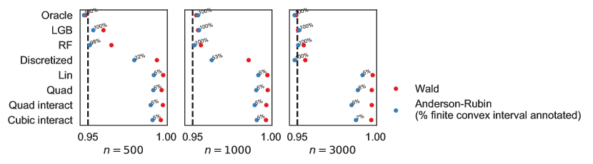
Figure 5: Wald and Anderson–Rubin coverage rates in the setting of Section C.1. The parenthesized values are the percentage empirical Anderson–Rubin intervals of the finite interval form.

We note that flexible estimators appear to be able to discover the complex nonlinear relationship $\mathbb{E}[D\mid W]$ and produce estimates of $\tau$ that perform well, whereas more traditional estimators appear to have some trouble estimating a strong first-stage, resulting in noisy and biased estimates of $\tau$. In particular, polynomial regression-based estimators generally have median-biased second stage coefficients with large variances, particularly if sample-splitting is employed. Among the linear-regression-based estimators, the discretization-based estimator appears to benefit significantly with larger sample sizes and sample-splitting. Unsurprisingly, the flexible estimators have superior measures of fit in $R^{2}$ and the first-stage $F$-statistics Figure 4.

Estimating the optimal instrument with inverse variance weighting appears to deliver modest benefits in improving the precision of the second-stage estimator when LightGBM and random forest are used to estimate the instrument, but the benefit is quite substantial when we consider the discretization-based estimator.

We report inference performance in Figure 5. Again, we see that the flexible methods (“machine learning methods” and, to a lesser extent, the discretization estimator) perform well, with both Wald and Anderson–Rubin intervals covering at close to the nominal level. Meanwhile, methods that fail to estimate a strong instrument produces confidence sets that are very conservative in the split-sample setting, and almost always produces Anderson–Rubin confidence sets which do not take a finite interval shape.

C.2 With covariates

We modify the above design by including covariates. Let

$$X=AW+V,$$

where $V\sim\mathcal{N}(0,I)$ and $A=\begin{bmatrix}1&0.4&0.3\\ 0.5&2&0.2\end{bmatrix},$ be two covariates: $X=[X_{0},X_{1}]^{\top}$. If $X_{0}>0$, then we flip $D$ with probability 0.3 to obtain $\tilde{D}$, and we let

$$\tilde{Y}=\tilde{D}+X^{\top}\begin{bmatrix}0.1\\ 0.3\end{bmatrix}+U.$$

as the modified outcome. As before, $\mathbb{E}[U\mid W]=0$ and the true effect is $\tau=1$. However, we note that the changes in the DGP means that the setting here and the setting in Section C.1 are similar but not directly comparable—it is not clear whether the setting here is easier or harder to estimate, compare to the setting in Section C.1.

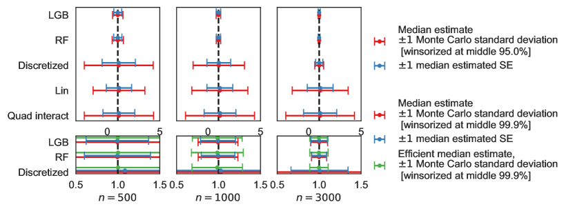
Notes: Median estimates, winsorized standard deviation, and median estimated standard error reported for a variety of estimators. The Monte Carlo standard deviations are computed from winsorized point estimates since the finite-sample variance of the linear IV estimator may not exist.

The estimators are split-sample IV estimators that differ in their construction of the instrument: LGB refers to using LightGBM, a gradient boosting algorithm; RF refers to using random forest; Discretized refers to discretizing $W_{0},W_{1},W_{2}$ into four levels at thresholds $-1,0,1$, and using all $4^{3}$ interactions as categorical covariates; Lin refers to linear regression with $W_{0},W_{1},W_{2}$ untransformed; Quad interact refers to quadratic regression with full interactions.

The bottom panel is a zoomed-in version of the best performing estimators. We also show the performance of the efficient estimator (estimating the optimal instrument with inverse-variance weighting) in the bottom panel in green.

Figure 6: Performance of a variety of estimators for $\tau$ in the setting of Section C.2

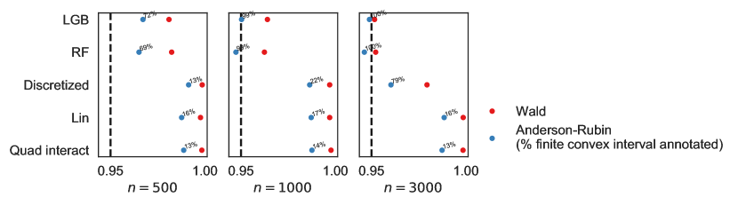
Figure 7: Wald and Anderson–Rubin coverage rates in the setting of Section C.2. The parenthesized values are the percentage empirical Anderson–Rubin intervals of the finite interval form.

We show the estimation performance in Figure 6 and inference performance in Figure 7, much like we did in Figures 3 and 5. Again, we generally have better performance for flexible methods, and polynomial regression methods do not appear to have comparable performance. In this case, it appears that when the sample size is small, even the machine learning based methods sometimes result in an estimated instrument that is weak. Moreover, interestingly, in this case, efficient methods do not produce appreciable improvement over methods without inverse variance weighting, for settings where LGB and RF are used to construct instruments. If anything, inverse variance weighting seems to do somewhat worse in finite samples, potentially due to additional noise in the estimation procedure.

Appendix D Interpretation under heterogeneous treatment effects

Suppose $\Upsilon(W_{i})=a(W_{i})[1,b(W_{i})]^{\prime}$ for some scalar functions $a,b$ with $a(\cdot)\geq 0$ and $\mathbb{E}[a(W_{i})]<\infty$. Then the corresponding linear IV estimand, using $\Upsilon$ as instrument, can be written as a weighted average of marginal treatment effects, a result due to Heckman and Vytlacil (2005), which we reproduce here:

$$\tau_{\Upsilon}=\int_{0}^{1}w(v)\cdot{\operatorname{MTE}_{a}(v)}\,dv\equiv\int_{0}^{1}w(v)\cdot\mathbb{E}\left[{\frac{a(W_{i})}{\mathbb{E}a(W_{i})}(Y_{1}-Y_{0})\mid V=v}\right]\,dv$$

where the weights are

$$w(v)\equiv\frac{\mathbb{E}\left[{a(W_{i})\tilde{b}(W_{i})\mathbbm{1}(\mu(W_{i})>v)}\right]}{\mathbb{E}[a(W_{i})\tilde{b}(W_{i})\mu(W_{i})]}\quad\tilde{b}(W_{i})\equiv b(W_{i})-\mathbb{E}\left[{\frac{a(W_{i})}{\mathbb{E}[a(W_{i})]}b(W_{i})}\right].$$

The weights $w(\cdot)$ integrate to 1 and are nonnegative whenever $b(W_{i})$ is a monotone transformation of $\mu(W_{i})$.

In the special case where $a(W_{i})=1$ and $b(W_{i})=\mu(W_{i})$, which corresponds to using the optimal instrument under identity weighting, the estimand is a convex average of marginal treatment effects. In the case where $a(W_{i})=1/\sigma^{2}(W_{i})$ and $b(W_{i})=\mu(W_{i})$, the estimand is a convex average of precision-weighted marginal treatment effects. In the heterogeneous treatment effects setting, we stress that efficiency comparisons are no longer meaningful, since the estimators do not converge to the same estimand. However, we nonetheless highlight the benefit of using an optimal instrument-based estimator compared to a standard linear IV estimator: Optimal instrument-based estimators are guaranteed to recover convex-weighted average treatment effects, where linear IV estimators with $W_{i}$ as the instrument may not.

References

- Ai and Chen (2003) Ai, C. and Chen, X. (2003). Efficient estimation of models with conditional moment restrictions containing unknown functions. Econometrica, 71 (6), 1795–1843.
- Ai and Chen (2007) — and — (2007). Estimation of possibly misspecified semiparametric conditional moment restriction models with different conditioning variables. Journal of Econometrics, 141 (1), 5–43.
- Ai and Chen (2012) — and — (2012). The semiparametric efficiency bound for models of sequential moment restrictions containing unknown functions. Journal of Econometrics, 170 (2), 442–457.
- Anderson et al. (1949) Anderson, T. W., Rubin, H. et al. (1949). Estimation of the parameters of a single equation in a complete system of stochastic equations. The Annals of Mathematical Statistics, 20 (1), 46–63.
- Andrews et al. (2019) Andrews, I., Stock, J. H. and Sun, L. (2019). Weak instruments in iv regression: Theory and practice. In Annual Review of Economics.
- Angrist and Frandsen (2019) Angrist, J. and Frandsen, B. (2019). Machine labor. Tech. rep., National Bureau of Economic Research.
- Angrist et al. (1999) Angrist, J. D., Imbens, G. W. and Krueger, A. B. (1999). Jackknife instrumental variables estimation. Journal of Applied Econometrics, 14 (1), 57–67.
- Angrist and Krueger (1991) — and Krueger, A. B. (1991). Does compulsory school attendance affect schooling and earnings? The Quarterly Journal of Economics, 106 (4), 979–1014.
- Angrist and Krueger (2001) — and — (2001). Instrumental variables and the search for identification: From supply and demand to natural experiments. Journal of Economic perspectives, 15 (4), 69–85.
- Angrist and Pischke (2008) — and Pischke, J.-S. (2008). Mostly harmless econometrics: An empiricist’s companion. Princeton university press.
- Antoine and Lavergne (2019) Antoine, B. and Lavergne, P. (2019). Identification-robust nonparametric inference in a linear iv model.
- Ash et al. (2019) Ash, E., Chen, D., Zhang, X., Huang, Z. and Wang, R. (2019). Deep iv in law: Analysis of appellate impacts on sentencing using high-dimensional instrumental variables. In Advances in Neural Information Processing Systems (Causal ML Workshop).
- Bai and Ng (2010) Bai, J. and Ng, S. (2010). Instrumental variable estimation in a data rich environment. Econometric Theory, pp. 1577–1606.
- Bekker (1994) Bekker, P. A. (1994). Alternative approximations to the distributions of instrumental variable estimators. Econometrica: Journal of the Econometric Society, pp. 657–681.
- Belloni et al. (2012) Belloni, A., Chen, D., Chernozhukov, V. and Hansen, C. (2012). Sparse models and methods for optimal instruments with an application to eminent domain. Econometrica, 80 (6), 2369–2429.
- Chamberlain (1987) Chamberlain, G. (1987). Asymptotic efficiency in estimation with conditional moment restrictions. Journal of Econometrics, 34 (3), 305–334.
- Chamberlain (1992) — (1992). Comment: Sequential moment restrictions in panel data. Journal of Business & Economic Statistics, 10 (1), 20–26.
- Chen and Pouzo (2012) Chen, X. and Pouzo, D. (2012). Estimation of nonparametric conditional moment models with possibly nonsmooth generalized residuals. Econometrica, 80 (1), 277–321.
- Chen and Pouzo (2015) — and — (2015). Sieve wald and qlr inferences on semi/nonparametric conditional moment models. Econometrica, 83 (3), 1013–1079.
- Chernozhukov et al. (2018) Chernozhukov, V., Chetverikov, D., Demirer, M., Duflo, E., Hansen, C., Newey, W. and Robins, J. (2018). Double/debiased machine learning for treatment and structural parameters.
- Chernozhukov et al. (2016) —, Escanciano, J. C., Ichimura, H., Newey, W. K. and Robins, J. M. (2016). Locally robust semiparametric estimation. arXiv preprint arXiv:1608.00033.
- Chernozhukov et al. (2015) —, Hansen, C. and Spindler, M. (2015). Post-selection and post-regularization inference in linear models with many controls and instruments. American Economic Review, 105 (5), 486–90.
- Currie et al. (2020) Currie, J., Kleven, H. and Zwiers, E. (2020). Technology and big data are changing economics: mining text to track methods. In AEA Papers and Proceedings, vol. 110, pp. 42–48.
- Dieterle and Snell (2016) Dieterle, S. G. and Snell, A. (2016). A simple diagnostic to investigate instrument validity and heterogeneous effects when using a single instrument. Labour Economics, 42, 76–86.
- Dikkala et al. (2020) Dikkala, N., Lewis, G., Mackey, L. and Syrgkanis, V. (2020). Minimax estimation of conditional moment models. arXiv preprint arXiv:2006.07201.
- Dufour (2003) Dufour, J.-M. (2003). Identification, weak instruments, and statistical inference in econometrics. Canadian Journal of Economics/Revue canadienne d’économique, 36 (4), 767–808.
- Escanciano and Li (2020) Escanciano, J. C. and Li, W. (2020). Optimal linear instrumental variables approximations. Journal of Econometrics.
- Friedman et al. (2001) Friedman, J., Hastie, T., Tibshirani, R. et al. (2001). The elements of statistical learning, vol. 1. Springer series in statistics New York.
- Hansen and Kozbur (2014) Hansen, C. and Kozbur, D. (2014). Instrumental variables estimation with many weak instruments using regularized jive. Journal of Econometrics, 182 (2), 290–308.
- Hartford et al. (2017) Hartford, J., Lewis, G., Leyton-Brown, K. and Taddy, M. (2017). Deep iv: A flexible approach for counterfactual prediction. In International Conference on Machine Learning, pp. 1414–1423.
- Heckman and Vytlacil (2005) Heckman, J. J. and Vytlacil, E. (2005). Structural equations, treatment effects, and econometric policy evaluation 1. Econometrica, 73 (3), 669–738.
- Horowitz and Lee (2007) Horowitz, J. L. and Lee, S. (2007). Nonparametric instrumental variables estimation of a quantile regression model. Econometrica, 75 (4), 1191–1208.
- Kaji (2019) Kaji, T. (2019). Theory of weak identification in semiparametric models. arXiv preprint arXiv:1908.10478.
- Le and Mikolov (2014) Le, Q. and Mikolov, T. (2014). Distributed representations of sentences and documents. In International conference on machine learning, pp. 1188–1196.
- Lei et al. (2018) Lei, J., G’Sell, M., Rinaldo, A., Tibshirani, R. J. and Wasserman, L. (2018). Distribution-free predictive inference for regression. Journal of the American Statistical Association, 113 (523), 1094–1111.
- Liu et al. (2020) Liu, R., Shang, Z. and Cheng, G. (2020). On deep instrumental variables estimate.
- Mackey et al. (2018) Mackey, L., Syrgkanis, V. and Zadik, I. (2018). Orthogonal machine learning: Power and limitations. In International Conference on Machine Learning, PMLR, pp. 3375–3383.
- Mikusheva and Sun (2020) Mikusheva, A. and Sun, L. (2020). Inference with many weak instruments. arXiv preprint arXiv:2004.12445.
- Newey and Powell (2003) Newey, W. K. and Powell, J. L. (2003). Instrumental variable estimation of nonparametric models. Econometrica, 71 (5), 1565–1578.
- Raskutti et al. (2011) Raskutti, G., Wainwright, M. J. and Yu, B. (2011). Minimax rates of estimation for high-dimensional linear regression over -balls. IEEE transactions on information theory, 57 (10), 6976–6994.
- Robinson (1988) Robinson, P. M. (1988). Root-n-consistent semiparametric regression. Econometrica: Journal of the Econometric Society, pp. 931–954.
- Severini and Tripathi (2012) Severini, T. A. and Tripathi, G. (2012). Efficiency bounds for estimating linear functionals of nonparametric regression models with endogenous regressors. Journal of Econometrics, 170 (2), 491–498.
- Staiger and Stock (1994) Staiger, D. and Stock, J. H. (1994). Instrumental variables regression with weak instruments. Tech. rep., National Bureau of Economic Research.
- Stock and Yogo (2005) Stock, J. H. and Yogo, M. (2005). Testing for weak instruments in linear iv regression. Identification and inference for econometric models: Essays in honor of Thomas Rothenberg, 80 (4.2), 1.
- Xu (2021) Xu, R. (2021). Weak Instruments with a Binary Endogenous Explanatory Variable. Tech. rep.