A WLAV-based Robust Hybrid State Estimation using Circuit-theoretic Approach
Abstract
For reliable and secure power grid operation, AC state-estimation (ACSE) must provide certain guarantees of convergence while being resilient against bad-data. This paper develops a circuit-theoretic weighted least absolute value (WLAV) based hybrid ACSE that satisfies these needs to overcome some of the limitations of existing ACSE methods. Hybrid refers to the inclusion of RTU and PMU measurement data, and the use of the LAV objective function enables automatic rejection of bad data while providing clear identification of suspicious measurements from the sparse residual vector. Taking advantage of linear construction of the measurement models in circuit-theoretic approach, the proposed hybrid SE is formulated as a LP problem with guaranteed convergence. To address efficiency, we further develop problem-specific heuristics for fast convergence. To validate the efficacy of the proposed approach, we run ACSE on large cases and compare the results against WLS-based algorithms. We further demonstrate the advantages of our solution methodology over standard commercial LP solvers through comparison of runtime and convergence performance.
Index Terms:
AC state estimation, bad data, least absolute value, L1-normI Introduction
Today’s central grid operators run AC state estimation (ACSE) at minute scale to gain situational awareness of the grid states. Network topology and grid measurements are inputs and grid states that include complex bus voltages and angles are produced as output. Furthermore, the output serves as the input to other critical grid analyses such as optimal power flow (OPF) and contingency analysis. It follows that for secure and reliable grid operation and control, robust ACSE is critical.
To ensure robustness, ACSE needs some resilience against faulty input measurements to promote reliable estimation. The grid today is highly susceptible to erroneous data from conventional sensors and networked PMUs due to disturbances (measurement device error, communication error) and malicious attacks. As a result, many methods have been proposed to make ACSE resilient from bad data. Most common amongst these are hypothesis tests that are based on post-processing of the weighted least square (WLS) problem residuals [1],[2],[3]. Within these algorithms, the identification of bad data is followed by adjusting suspicious measurements and rerunning ACSE until residuals are satisfactory. Possible ways of adjustments include removing bad data, modifying [3] bad data, or iterative reweighted least square method [2], where weights on suspicious measurements are set to lower values. Clearly, the iterative re-running of the ACSE problem incurs a computational burden. Other robust estimators include least median of squares [4], yet it is not widely adopted due to numerical difficulty in handling the median.
Built upon the assumption that bad data are typically sparse, researchers have also proposed the use of weighted least absolute value (WLAV) in the objective function [5][6][7][8]. The WLAV based methods enable automatic rejection of bad data, eliminating the need of iterative re-runs while providing clear identification of suspicious measurements from the sparse residual vector. Despite this desirable property, the non-differentiable L1-norm terms in the WLAV approach introduces additional complexity. At present, two approaches to WLAV-ACSE exist: i) those that solve highly non-convex ACSE due to inclusion of power measurements from conventional RTUs [9]; and ii) those that are formulated as a linear programming (LP) problem [7][8] with the assumption that network only consists of PMUs. These convex WLAV formulations based solely on PMUs take advantage of linear relationship between phasor data and grid states; however, assuming PMU-observability of the network is highly unrealistic for grids today.
To be readily applicable to grids today, ACSE must include conventional RTUs. Unfortunately, most methods that include conventional RTUs (hybrid or otherwise) correspond to ACSE methods with highly complex and non-convex solution space that presents convergence challenges and high residuals. To address these problems, there has been some work on convex relaxations of ACSE methods (applicable to WLAV as well). For instance, [10] convexifies the problem by reformulating the voltage magnitude , phase angle , and product of and , in semidefinite programming (SDP) form, through matrix transformation; however the method fails to scale effectively to large scale networks. More recently to overcome the convergence and high residual limitations, the researchers in [11],[12] proposed a circuit theoretic ACSE approach that reduces the problem to an equality constrained quadratic programming (QP) problem by creating linear measurement models following a ‘sensitivity’ based mapping of conventional grid measurements. This approach provides a convex hybrid ACSE forumulation that is scalable to large networks, but it is not implicitly resilient to bad data.
In this paper we extend the work in [11],[12] to create a convex weighted least absolute value (WLAV) based hybrid SE. Exploiting the linear modeling framework for both conventional RTUs and PMUs in [11],[12], we formulate the hybrid SE as a linear programming (LP) problem that provides implicit bad data detection. Also to solve the problem efficiently, this paper develops circuit-theoretic solution methodology with primal-dual interior point (PDIP) approach [13] that is aided by heuristics for fast convergence on large-scale systems. To demonstrate the efficacy of this approach, results are presented for ACSE experiments on large networks to compare efficiency and performance against the simplex method and other general-purpose PDIP solvers.
II Circuit Formulation of SE Problem
II-A Equivalent Circuit Formulation (ECF)
A circuit-theoretic formulation for power flow and grid optimizations was developed in [14], [15]. Instead of describing components with power-based ‘PQV’ parameters, this framework models each component within the power grid as an equivalent circuit characterized by its I-V relationship. The I-V relationships can represent both transmission and distribution grids without loss of generality and, when applied to SE, can include measurement data naturally without incurring the non-linearity associated with state variables. For computational analyticity, the complex relationships are split into real and imaginary sub-circuits whose nodes correspond to power system buses.
II-B Incorporating PMU and RTU
Today, critical states of bulk energy systems (BES) are sensed by conventional remote terminal units (RTUs) and networked phasor measurement units (PMUs) and these measured parameters are continuously sent to grid control rooms through secure telemetry. We have previously shown in [14] that the complete power grid model can be represented as an aggregated equivalent circuit. Now to include RTU and PMU measurements into this circuit model, we apply Substitution Theorem that posits that any measured element in the grid can be replaced with voltage and current sensor measurements from that component or the flow element without changing the overall solution. However, due to inherent noise in the measurement devices, for each measurement model we include an additional slack injection variable, to satisfy Kirchhoff’s current law (KCL). We have previously shown in [11],[12] that with linear measurements models, the ECF framework maps the entire measurement dependent power grid model into a linear equivalent circuit representation of the entire system.
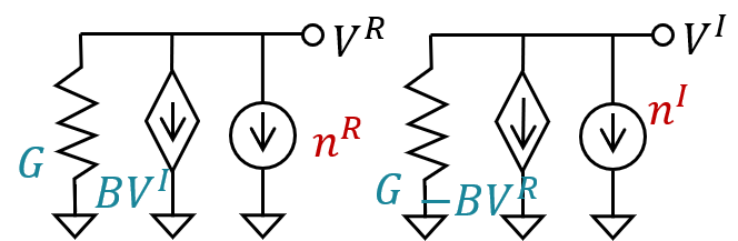
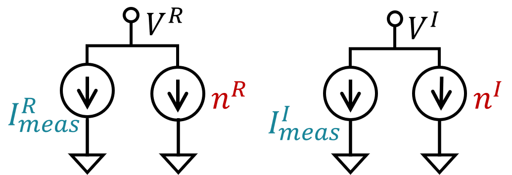
We briefly describe the construction of circuit-theoretic measurement models for RTUs and PMUs here (see [11],[12] for details). Figure 1(a) represents the measurement circuit model for an RTU. In the model, the original injection measurements (voltage magnitude , and power injection ) are mapped into sensitivities () such that the I-V relationship is satisfied to obtain the linear circuit model. PMU measurements () are intrinsically linear under a rectangular coordinate framework and the linear circuit model is characterized by independent current and voltage sources (see Figure 1(b)). Models for line flow measurements from RTU and PMU have been created in a similar way. Meanwhile, to account for possible measurement errors, the models have included noise terms, or slack variables, which are to be minimized.
III WLAV-SE definition and solution
III-A Problem Definition
Even though existing circuit-theoretic WLS-based ACSE methods [11] provide robust convergence guarantees, they lack an implicit bad-data detection capability that is becoming increasingly critical due to higher likelihood of coordinated attacks on grid measurements and naturally occurring faulty meters. Today, WLS-based SE applies a post-processing based method to perform bad data analysis by hypothesis test. This requires examination of residuals followed by updating and rerunning of SE in case any suspicious measurements are determined. Under the presence of bad data, such a methodology even with the existence of closed-form solution can face high computational burden. Moreover, since they are prone to false negatives, these methods can have undetected bad measurements that adversely impact the SE solution.
To enhance the intrinsic reliability of the SE solution and eliminate the need for rerunning SE recursively, this paper develops a circuit-theoretic weighted least-absolute value (WLAV) estimator. By enforcing sparse value for residuals, this method can implicitly detect bad-data without the need for recursive re-runs of SE. Moreover, with the sparse residual vector capturing the pattern and impact of (sparse) measurement error, the solution to WLAV based SE is less corrupted and more reliable. And while existing WLAV SE methods that include both PMUs and RTUs have a non-convex complex solution space, we formulate a convex WLAV SE method with the linear measurement models described in Section II-B. Mathematical formulation is described as follows:
| (1a) | |||
| s.t. KCL equations:
PMU bus : | |||
| (1b) | |||
| (1c) | |||
| RTU bus : | |||
| (1d) | |||
| (1e) | |||
| Zero-injection bus : | |||
| (1f) | |||
| (1g) | |||
| PMU line flow on line : | |||
| (1h) | |||
| (1i) | |||
| RTU line flow on line q: | |||
| (1j) | |||
| (1k) | |||
where is a diagonal matrix of weights, is the state vector containing real and imaginary voltage variables, refers to real/imaginary, is the admittance matrix, and refers to the bus where the line flow measurement device is metering.
Clearly, this is mathematically a linear programming (LP) problem for hybrid state estimation. The convex nature of the problem dispels any concerns regarding convergence issues even with conventional measurements. And built on the assumption that bad data are sparse, the solution to this problem automatically rejects them to return a reliable estimation. We now evaluate various solution methodologies for this problem and propose an algorithm with superior speed and robustness.
III-B Fast and Robust Solution Methodology
This section describes our solution methodology for efficiently solving the problem described in (1k). It applies a primal-dual interior point (PDIP) algorithm [13] with novel problem-specific heuristics to achieve robust and fast convergence. This approach has superior convergence properties over simplex-based [16] algorithms for large-scale problems. The Simplex method is generally better suited for smaller problems since it traverses through a set of vertices of the feasible space until the optimal solution is found. However, as the problem size increases, the number of vertices grow exponentially, making the method impractical for larger networks.
In the PDIP approach, to obtain the optimal solution, we solve the set of perturbed KKT conditions that are necessary and sufficient for optimality under convexity and strong duality. Compared with the exponential computational complexity of the Simplex method, this approach has proven to be effective on large-scale problems [13], with its worst-case complexity being polynomial to problem dimension.
To apply PDIP algorithm to Problem (1k), a standard transformation [6],[13] is performed to convert the non-differentiable L1 terms into differentiable format as below:
| (2a) | |||
| (2b) |
Standard toolboxes can be used to solve the problem described in (2). These include CVXOPT [17], SciPy [18], etc. Yet the (speed) performance of these solvers is limited for large grid cases. Therefore, to further improve the efficiency, we solve the perturbed KKT conditions with problem-specific limiting heuristics. Taking into account that the problem is convex and only local nonlinearity exists in the complementary slackness component of the perturbed KKT conditions, we apply simple step-limiting only on dual variables (corresponding to inequalities) and to make each iteration update faster and more efficient. This approach moves away from standard filter line-search algorithms [17] used by other generic tools. The proposed algorithm is shown in Algorithm 1.
III-C Comparison and Interpretation of WLAV-SE versus WLS-SE
We compared the proposed circuit-theoretic WLAV approach against the circuit-theoretic and traditional WLS approaches. Mathematically, the proposed WLAV problem defined in Section III-A is equivalent to the following form:
| (3a) | |||
In contrast, our previous work [11] has formulated hybrid SE as a quadratic programming (QP) problem
| (4a) | |||
And the classical ’PQV’ based WLS-SE[19] is a direct minimization of measurement error, where is the vector of original measurements and is the non-linear relationship between and :
| (5) |
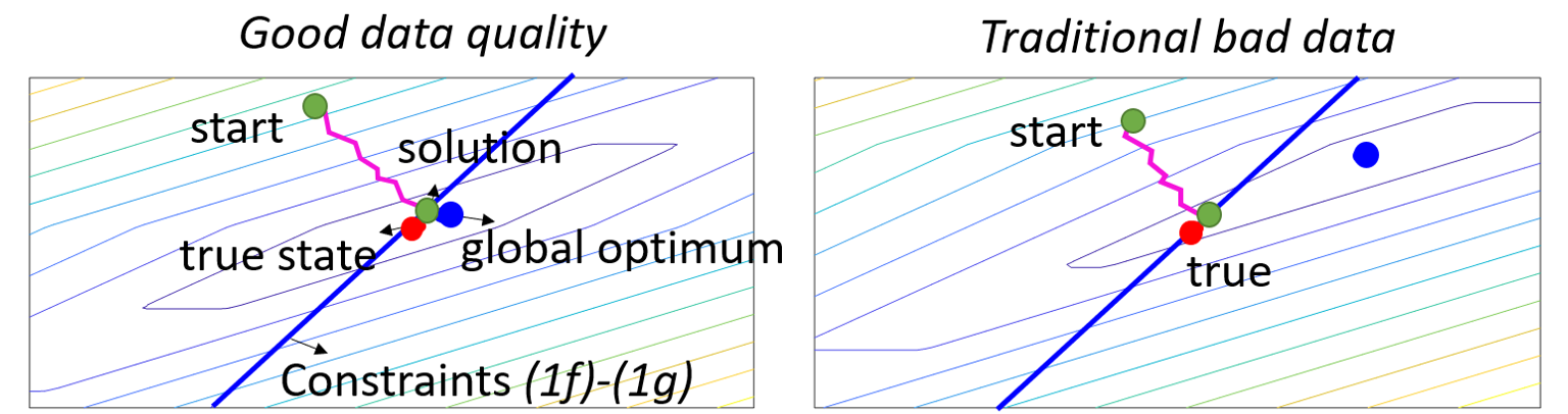
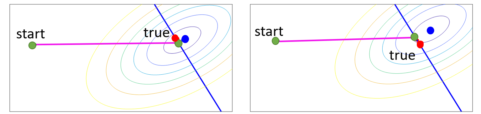
Figure 2 presents the solution trajectory of these different SE formulations. Through comparison from an optimization viewpoint, it is clear that both our proposed method and our previous work [11] benefit from convexity and the additional error-free zero-injection constraints. In contrast, the classical WLS method, which is non-convex and iterative, suffers from convergence to local minimum and saddle points. In addition to being convex, the proposed WLAV method provides additional benefits of implicit bad-data analysis, as justified by the results in later Section (see Table II). This not available with WLS-based methods in general.

IV Results
We conducted experiments to validate our proposed method for rejecting bad data. We constructed synthetic RTU injection and line flow measurements by adding Gaussian noise (std=0.001) to power flow solutions. To construct synthetic bad data, we added large deviations to a few randomly selected measurements. To evaluate the accuracy of the proposed estimation method, we use root mean square error as the performance metric:
Table I shows comparison results for IEEE 14 bus network, where bad measurements exist on bus 6 and 14. From general observation of nodal residuals that benefit from the LAV objective, our proposed method successfully identifies the location of bad data while the WLS method in [11] fails to do so. Furthermore, smaller shows the solution from WLAV SE is more accurate, validating its capability to reject bad data automatically.
| Bus ID | Proposed WLAV-SE | WLS-SE[11] |
| 1 | 0 | 0 |
| 2 | 0.009 | 0.124 |
| 3 | 0 | 0.115 |
| 4 | 0.065 | 0.121 |
| 5 | 0 | 0.131 |
| 6 (bad) | 1.095 | 0.313 |
| 8 | 0.002 | 0.027 |
| 9 | 0.0 | 0.090 |
| 10 | 0.0 | 0.113 |
| 11 | 0.0 | 0.059 |
| 12 | 0.024 | 0.155 |
| 13 | 0.0 | 0.199 |
| 14 (bad) | 0.658 | 0.306 |
| RMSE | 0.042 | 0.090 |
Next, we ran the proposed WLAV-SE on larger networks and compared our solution methodology against some standard optimization toolboxes [17][18]. In each test network, bad data was added on 5 randomly selected locations (data is available in https://github.com/ohCindy/LAV-SE-synthetic-data.git).
| CASE |
|
|
|
|
|||||||||||
|---|---|---|---|---|---|---|---|---|---|---|---|---|---|---|---|
| 14 |
|
|
|||||||||||||
| 118 |
|
|
|||||||||||||
| 2383wp |
|
|
|||||||||||||
| 6468rte |
|
|
|||||||||||||
| 9241pegase | Fails |
|
* We compare 4 methods: The traditional WLS based SE in MATPOWER, and WLAV-based SE defined in Section III-A implemented by 3 different LP solvers: Simplex method in SciPy toolbox, interior-point (IP) method in CVXOPT toolbox, and IP method by our proposed solver
* ’os’ refers to optimization status reported by standard tooxbox. ’optimal’ means optimal solution reached successfully, ’infeasible’ means problem appears to be infeasible for the toolbox, ’unknown’ means algorithm optimization terminated due to maximum iterations or numerical difficulties
Table II compares the accuracy of estimation, by using the metric. The results show that WLAV-based ACSE (see columns 3,4,5 in Table II) provides superior estimates over WLS-based ACSE (see column 2 in Table II).
| CASE |
|
|
|
||||||
|---|---|---|---|---|---|---|---|---|---|
| 14 |
|
|
0.250s, 19 iters | ||||||
| 118 |
|
|
|
||||||
| 2383wp |
|
|
|
||||||
| 6468rte | Fails |
|
|
||||||
| 9241pegase | Fails |
|
|
Additional results in Table III show that the proposed method has faster convergence for large cases when compared against baseline LP solvers. In general, CVXOPT takes fewer iterations to converge but each iteration is expensive due to the delicate computation of step-size and centering parameter to choose a proper search direction. In comparison, the proposed method, with simple heuristics, makes each iteration cheaper but requiring more iterations to converge. In contrast to both solvers, convergence of Simplex method significantly deteriorates when network size increases, which validates its limitation as stated in Section III-B.
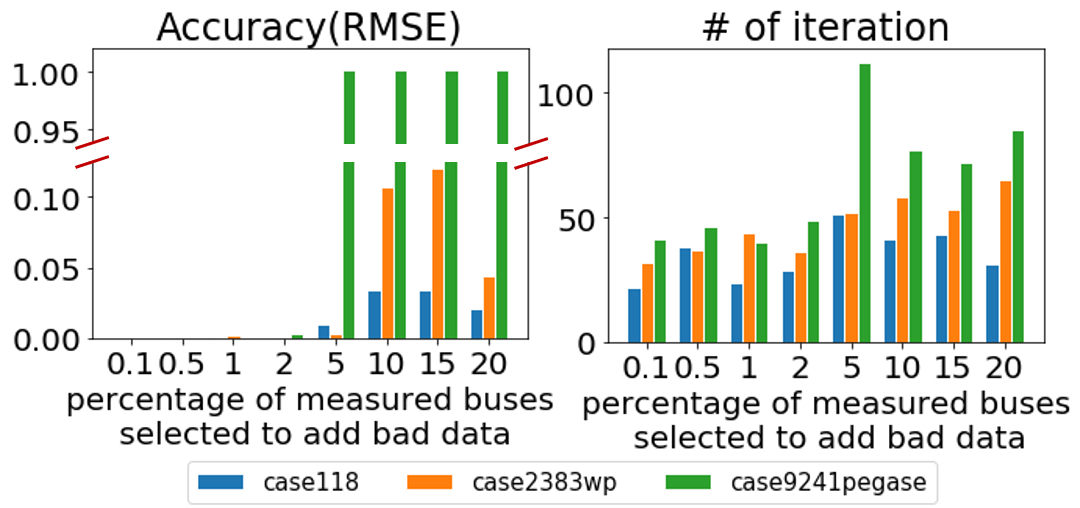
In the final experiment, we explore how our proposed method performs as the amount of bad data increases. Results (see Figure 3) show that the convergence efficiency (#iterations) remains stable under increasing bad-data samples, whereas the solution quality (accuracy) is stable for up to 5% penetration of bad measurement buses and starts to degrade thereafter. With high penetration of bad data the property of sparse residual is not well preserved, which violates the basic assumption of all LAV methods. However, given that non-interactive bad data are highly sparse in reality, our approach is practical and can robustly reject sparse bad data in a manner that is superior to classical methods, like -test[1] which is less effective even for more than single bad data.
V Conclusion
This paper presents a hybrid state estimation built on a circuit-theoretic foundation and models. Benefits include:
-
•
Guaranteed convergence due to formulation as a linear programming (LP) problem
-
•
Intrinsic resilience against bad-data due to use of a least absolute value objective that produces sparse residual
-
•
Fast convergence due to the use of problem specific heuristics for the solution engine
Furthermore, the proposed SE approach that is directly applicable to both transmission and distribution grids is also generalizable to parallel compute techniques; a key need for tomorrow with merging transmission and distribution grids.
Acknowledgment
This work was supported in part by the National Science Foundation (NSF) under contract ECCS-1800812.
References
- [1] E. Handschin, F. C. Schweppe, J. Kohlas, and A. Fiechter, “Bad data analysis for power system state estimation,” IEEE Transactions on Power Apparatus and Systems, vol. 94, no. 2, pp. 329–337, 1975.
- [2] R. C. Pires, A. S. Costa, and L. Mili, “Iteratively reweighted least-squares state estimation through givens rotations,” IEEE Transactions on Power Systems, vol. 14, no. 4, pp. 1499–1507, 1999.
- [3] A. Monticelli and A. Garcia, “Reliable bad data processing for real-time state estimation,” IEEE Transactions on Power Apparatus and Systems, no. 5, pp. 1126–1139, 1983.
- [4] L. Mili, V. Phaniraj, and P. J. Rousseeuw, “Least median of squares estimation in power systems,” IEEE Transactions on Power Systems, vol. 6, no. 2, pp. 511–523, 1991.
- [5] S. Soliman and M. El-Hawary, “Measurement of power systems voltage and flicker levels for power quality analysis: a static lav state estimation based algorithm,” International journal of electrical power & energy systems, vol. 22, no. 6, pp. 447–450, 2000.
- [6] W. W. Kotiuga and M. Vidyasagar, “Bad data rejection properties of weughted least absolute value techniques applied to static state estimation,” IEEE Transactions on Power Apparatus and Systems, no. 4, pp. 844–853, 1982.
- [7] M. Göl and A. Abur, “Lav based robust state estimation for systems measured by pmus,” IEEE Transactions on Smart Grid, vol. 5, no. 4, pp. 1808–1814, 2014.
- [8] Y. Lin and A. Abur, “Robust state estimation against measurement and network parameter errors,” IEEE Transactions on power systems, vol. 33, no. 5, pp. 4751–4759, 2018.
- [9] H. Singh, F. L. Alvarado, and W. . E. Liu, “Constrained lav state estimation using penalty functions,” IEEE Transactions on Power Systems, vol. 12, no. 1, pp. 383–388, 1997.
- [10] Y. Weng, M. D. Ilić, Q. Li, and R. Negi, “Convexification of bad data and topology error detection and identification problems in ac electric power systems,” IET Generation, Transmission & Distribution, vol. 9, no. 16, pp. 2760–2767, 2015.
- [11] S. Li, A. Pandey, S. Kar, and L. Pileggi, “A circuit-theoretic approach to state estimation,” arXiv preprint arXiv:1911.05155, 2019.
- [12] A. Jovicic, M. Jereminov, L. Pileggi, and G. Hug, “An equivalent circuit formulation for power system state estimation including pmus,” in 2018 North American Power Symposium (NAPS). IEEE, 2018, pp. 1–6.
- [13] K. Koh, S.-J. Kim, and S. Boyd, “An interior-point method for large-scale l1-regularized logistic regression,” Journal of Machine learning research, vol. 8, no. Jul, pp. 1519–1555, 2007.
- [14] A. Pandey, M. Jereminov, M. R. Wagner, D. M. Bromberg, G. Hug, and L. Pileggi, “Robust power flow and three-phase power flow analyses,” IEEE Transactions on Power Systems, vol. 34, no. 1, pp. 616–626, 2018.
- [15] M. Jereminov, A. Pandey, and L. Pileggi, “Equivalent circuit formulation for solving ac optimal power flow,” IEEE Transactions on Power Systems, vol. 34, no. 3, pp. 2354–2365, 2018.
- [16] G. B. Dantzig, Linear programming and extensions. Princeton university press, 1998, vol. 48.
- [17] L. Vandenberghe, “The cvxopt linear and quadratic cone program solvers,” Online: http://cvxopt. org/documentation/coneprog. pdf, 2010.
- [18] P. Virtanen, R. Gommers, T. E. Oliphant, M. Haberland, T. Reddy, D. Cournapeau, E. Burovski, P. Peterson, W. Weckesser, J. Bright et al., “Scipy 1.0: fundamental algorithms for scientific computing in python,” Nature methods, vol. 17, no. 3, pp. 261–272, 2020.
- [19] F. C. Schweppe and J. Wildes, “Power system static-state estimation, part i: Exact model,” IEEE Transactions on Power Apparatus and systems, no. 1, pp. 120–125, 1970.