$(f,\Gamma)$-Divergences: Interpolating between $f$-Divergences and Integral Probability Metrics

Abstract

We develop a rigorous and general framework for constructing information-theoretic divergences that subsume both $f$-divergences and integral probability metrics (IPMs), such as the $1$-Wasserstein distance. We prove under which assumptions these divergences, hereafter referred to as $(f,\Gamma)$-divergences, provide a notion of ‘distance’ between probability measures and show that they can be expressed as a two-stage mass-redistribution/mass-transport process. The $(f,\Gamma)$-divergences inherit features from IPMs, such as the ability to compare distributions which are not absolutely continuous, as well as from $f$-divergences, namely the strict concavity of their variational representations and the ability to control heavy-tailed distributions for particular choices of $f$. When combined, these features establish a divergence with improved properties for estimation, statistical learning, and uncertainty quantification applications. Using statistical learning as an example, we demonstrate their advantage in training generative adversarial networks (GANs) for heavy-tailed, not-absolutely continuous sample distributions. We also show improved performance and stability over gradient-penalized Wasserstein GAN in image generation.

Keywords $f$-divergences  $\cdot$ Integral probability metrics  $\cdot$ Wasserstein metric  $\cdot$ Variational representations  $\cdot$ GANs

1 Introduction

Divergences and metrics provide a notion of ‘distance’ between multivariate probability distributions, thus allowing for comparison of models with one another and with data. Divergences are used in many theoretical and practical problems in mathematics, engineering, and the natural sciences, ranging from statistical physics, large deviations theory, uncertainty quantification and statistics to information theory, communication theory, and machine learning. In this work, we introduce and study what we term the $(f,\Gamma)$-divergences, denoted by $D_{f}^{\Gamma}$ and defined by the variational expression

$$D_{f}^{\Gamma}(Q\|P)\equiv \sup_{g\in\Gamma}\left\{E_{Q}[g]-\Lambda_{f}^{P}[g]\right\}\,,$$ (1)

$$\Lambda_{f}^{P}[g]\equiv \inf_{\nu\in\mathbb{R}}\left\{\nu+E_{P}[f^{*}(g-\nu)]\right\}\,,$$ (2)

where $Q$ and $P$ are probability measures, $f$ is a convex function with $f(1)=0$, $f^{*}$ denotes the Legendre Transform (LT) of $f$, and $\Gamma\subset\mathcal{M}_{b}(\Omega)$ is an appropriate function space. The resemblance to the variational representation of the $f$-divergence is evident (see Eq. (4) below), however, the additional optimization over shifts $\nu$ in (2), which is motivated by the Gibbs variational principle [1], will enable the derivation of many theoretical properties of the $(f,\Gamma)$-divergence. In the special case of the Kullback-Leibler (KL) divergence, $\Lambda_{f}^{P}[g]$ is exactly the cumulant generating function that arises in the Donsker-Varadhan variational formula [2]. We will show that the $(f,\Gamma)$-divergences are related to, interpolate between, and inherit key properties from both the $f$-divergences and the integral probability metrics (IPMs). To motivate the definition in (1), we first recall the definition and basic properties of $f$-divergences and IPMs.

The family of $f$-divergences includes among others the KL divergence [3], the total variation distance, the $\chi^{2}$-divergence, the Hellinger distance, and the Jensen-Shannon divergence [4, 5]. The $f$-divergence between two probability measures $Q$ and $P$ induced by a convex function $f$ satisfying $f(1)=0$ is defined by

$$D_{f}(Q\|P)\equiv E_{P}[f(dQ/dP)]\,.$$ (3)

This definition assumes absolute continuity between $Q$ and $P$, $Q\ll P$, which in particular means that the support of $Q$ is included in the support of $P$. The estimation of an $f$-divergence directly from (3) is challenging since it requires knowledge of the likelihood ratio (i.e., Radon-Nikodym derivative) $dQ/dP$, such as when working within a parametric family, or of a reasonable approximation to $dQ/dP$, usually through histogram binning, kernel density estimation [6, 7], or through $k$-nearest neighbor approximation [8]. However, parametric methods greatly restrict the collection of allowed models, resulting in reduced expressivity, whereas non-parametric likelihood-ratio methods do not scale efficiently with the dimension of the data [9]. To address such challenges, statistical estimators which are based on variational representations of divergences have recently been introduced [10, 11].

Variational representation formulas for divergences, often referred to as dual formulations, convert divergence estimation into, in principle, an infinite-dimensional optimization problem over a function space. A typical example of a variational representation is the LT representation of the $f$-divergence between $Q$ and $P$, given by [12, 10]

$$D_{f}(Q\|P)=\sup_{g\in\mathcal{M}_{b}(\Omega)}\big{\{}E_{Q}[g]-E_{P}[f^{*}(g)]\big{\}}\,.$$ (4)

Such representations offer a useful mathematical tool to measure statistical similarity between data collections as well as to build, train, and compare complex probabilistic models. The main practical advantage of variational formulas is that an explicit form of the probability distributions or their likelihood ratio, $dQ/dP$, is not necessary. Only samples from both distributions are required since the difference of expected values in (4) can be approximated by statistical averages. In practice, the infinite-dimensional function space has to be approximated or even restricted. One of the first attempts was the restriction of the function space to a reproducing kernel Hilbert space (RKHS) and the corresponding kernel-based approximation in [10]. More recently, the optimization (4) has been approximated using flexible regression models and particularly by neural networks [11] and these techniques are widely used in the training of generative adversarial networks (GANs) [13, 14, 15, 16]. Variational representations of divergences have also been used to quantify the model uncertainty in a probabilistic model (arising, e.g., from insufficient data and partial expert knowledge). For instance, applying the $f$-divergence formula (4) to $cg-\nu$, solving for $E_{Q}[g]$, and optimizing over $c>0$, $\nu\in\mathbb{R}$ leads to the uncertainty quantification (UQ) bound [17, 18]

$$E_{Q}[g]\leq\inf_{c>0}\left\{\frac{1}{c}\Lambda_{f}^{P}[cg]+\frac{1}{c}D_{f}(Q\|P)\right\}\,.$$ (5)

Similarly, one can obtain a corresponding lower bound for any quantity of interest $g\in\mathcal{M}_{b}(\Omega)$. The UQ inequality (5) bounds the uncertainty in the expectation of $g$ under an alternative model $Q$ in terms of expectations under the baseline model $P$ and the discrepancy between $Q$ and $P$ (quantified via $D_{f}(Q\|P)$). Further discussion of the general connection between variational characterizations of divergences and UQ can be found in [19, 20, 21, 22, 23, 24, 25, 26].

Integral probability metrics are defined directly in terms of a variational formula [27, 28], generalizing the Kantorovich–Rubinstein variational formula for the Wasserstein metric [29]. More specifically, they are defined by maximizing the differences of respective expected values over a function space $\Gamma$,

$$W^{\Gamma}(Q,P)=\sup_{g\in\Gamma}\big{\{}E_{Q}[g]-E_{P}[g]\big{\}}\,,$$ (6)

and we refer to this object as the $\Gamma$-IPM. Despite the name, IPMs are not necessarily metrics in the mathematical sense unless further assumptions on $\Gamma$ are made. This will not be an issue for us going forward, as we are not focused on the metric property; we will be concerned with the divergence property, as defined in Section 2.1 below. Examples of IPMs include: the total variation metric, which is derived when the function space $\Gamma$ is the unit ball in the space of bounded measurable functions; the Wasserstein, metric where $\Gamma$ is the space of Lipschitz continuous functions with Lipschitz constant less than or equal to one; the Dudley metric, where the function space $\Gamma$ is the unit ball in the space of bounded and Lipschitz continuous functions; and the maximum mean discrepancy (MMD), where $\Gamma$ is the the unit ball in a RKHS, see also [27, 28, 30]. The definition of an IPM through the variational formula (6) leads to straightforward and unbiased statistical estimation algorithms [30]. Furthermore, the Wasserstein metric applied to generative adversarial networks (GANs) is known to substantially improve the stability of the training process [14, 16], while MMD offers one of the most reliable two-sample tests for high dimensional statistical distributions [31].

In summary, there are two fundamental mathematical ingredients involved in variational formulas for $f$-divergences and IPMs, with both families having their own strengths and weaknesses.

1. The Objective Functional: The objective functional in a variational representation is the quantity being maximized, namely $E_{Q}[g]-E_{P}[f^{*}(g)]$ for the $f$-divergences and $E_{Q}[g]-E_{P}[g]$ for the IPMs. The former depends on $f$ and for appropriate $f$’s it is strictly concave in $g$, while the latter is the same for all IPMs and is linear in $g$. Stronger convexity/concavity properties could result in improved statistical learning, estimation, and convergence performance. The ability to vary the objective functional by choosing $f$ also allows one to tailor the divergence to the data source, e.g., for heavy tailed data. Finally, note that alternative objective functionals can yield the same divergence [1, 32, 11, 26], and their careful choice can have a substantial impact on their statistical estimation [11, 32, 26].

2. The Function Space: This is the space over which the objective functional is optimized. In (4), it is the same function space for all $f$-divergences, namely $\mathcal{M}_{b}(\Omega)$, while the choice of function space $\Gamma$ is what defines an IPM in (6). The choice of $\Gamma$ has a profound impact on the properties of a divergence, e.g., the ability to meaningfully compare not-absolutely continuous distributions.

As we will show, the properties of the $(f,\Gamma)$-divergences can be tailored to the requirements of a particular problem through the choice of the objective functional (via $f$) and the function space $\Gamma$. The need for such a flexible family of divergences that combines the strengths of both $f$-divergences and IPMs is motivated by problems in machine learning and UQ, where properties of the data source or baseline model dictate the requirements on $f$ and $\Gamma$, e.g., the $f$-divergence UQ bound (5) is unable to treat structurally different alternative models $Q$, which can easily be mutually singular with $P$, as $D_{f}(Q\|P)=\infty$ under a loss of absolute continuity; similar issues appear in GANs, [14].

Related approaches include the recent studies [33, 34, 35, 36, 37, 25, 38]. In [35] the authors studied the use of spectral normalization to impose a Lipschitz constraint on the discriminator of a GAN; this is an example of (1) with a particular choice of function space. In [36], the authors proposed a class of objective functionals with an additional optimization layer, aiming to bridge the gap between the variational formulas for $f$-divergences and Wasserstein metrics and applied it to adversarial training of generative models. However, the paper does not provide a rigorous connection to the Wasserstein metric, since the function space appearing in their main Theorem 1 cannot include a Lipschitz constraint. This is in contrast to their practical implementation in Algorithm 1, which does employ a Lipschitz constraint. Our approach bridges this gap between theory and practice, as we are able to explicitly handle Lipschitz function spaces. Finally, our approach does not require the introduction of a third neural network, no matter what the choice of $f$-divergence may be. On the other hand, the authors in [25] developed a variational formula for general function spaces in the case of the KL divergence, providing a systematic and rigorous interpolation between KL divergence and IPMs. Definition (1) can be also viewed as a regularization of the classical $f$-divergences, and related objects have also been introduced and studied in [33, 37, 34, 38]. While there is some overlap with several prior works, the aim of this paper is to provide a systematic and rigorous development of the $(f,\Gamma)$-divergences, focusing on a number of new properties that are potentially beneficial in learning and UQ applications. Specifically:

1. We derive conditions under which $D_{f}^{\Gamma}$ has the divergence property, and thus provide a well-defined notion of ‘distance’ (Part 4 of Theorem 2.8 and Part 4 of Theorem 2.15). One key novelty is the introduction of the object (2) which is critical in the proof of this property.

2. We show that $D_{f}^{\Gamma}$ interpolates between the $f$-divergence and $\Gamma$-IPM in the sense of infimal convolutions, including existence of an optimizer (Parts 1 and 2 of Theorem 2.15). Again, (2) plays a critical role here.

3. Using the infimal convolution formula, we derive a mass-redistribution/mass-transport interpretation of the $(f,\Gamma)$-divergences (Section 3).

4. We show that the family of $(f,\Gamma)$-divergences includes $f$-divergences and $\Gamma$-IPMs in suitable asymptotic limits (Theorem 2.17).

5. The relaxation of the hard constraint $g\in\Gamma$ in (1) to a soft-constraint penalty term is presented in Theorem 4.4. This is a generalization of the gradient penalty method for Wasserstein metrics [16] to a much larger class of objective functionals and penalties and a key tool in designing numerically efficient implementations while still preserving the divergence property.

6. Relaxation of the condition $\Gamma\subset\mathcal{M}_{b}(\Omega)$ in (1), i.e., allowing $\Gamma$ to contain appropriate unbounded functions, is addressed in Theorem 5.5. This is a necessary point when employing neural network estimation with unbounded activation functions.

7. We show that the $(f,\Gamma)$-divergences inherit several properties from both $f$-divergences and the IPMs. The primary advantage inherited from IPMs is the ability to compare distributions which are not absolute continuous. The primary advantages inherited from the $f$-divergence are the strict concavity of the objective functional with respect to the test function, $g$, and the ability to compare heavy-tailed distributions (Section 6).

When combined, these advantages establish a divergence with better convergence and estimation properties. We numerically demonstrate these merits in the training of GANs. In Section 6.2, we show that the proposed divergence is capable of adversarial learning of lower dimensional sub-manifold distributions with heavy tails. In this example, both $f$-GAN [15] and Wasserstein GAN with gradient penalty (WGAN-GP) [16] fail to converge or perform very poorly. Furthermore, in Section 6.3 we present improvements over WGAN-GP and WGAN with spectral-normalization (WGAN-SN) [35], as measured by the inception score [39] and FID score [40] (two standard performance measures), in real datasets and particularly in CIFAR-10 [41] image generation. Interestingly, the training stability is significantly enhanced when using the proposed $(f,\Gamma)$-divergence, as compared to WGAN, which is evident from the fact that increasing the learning rate (i.e., stochastic gradient descent step size) eventually results in the collapse of WGAN but has comparatively little impact on our newly proposed method. We conjecture that this is due to the strict concavity of the objective functional of the $(f,\Gamma)$-divergence. We refer to these new proposed GANs which are based on $(f,\Gamma)$-divergences as $(f,\Gamma)$-GANs.

The organization of the paper is as follows. The key properties of the $(f,\Gamma)$-divergences are presented in Section 2. The mass-redistribution/mass-transport interpretation of the $(f,\Gamma)$-divergences is discussed in Section 3. Section 4 develops a general theory of soft-constraint penalization. Section 5 provides conditions under which the function space $\Gamma$ can be expanded to contain unbounded functions. The application of the $(f,\Gamma$)-divergences in adversarial generative modelling is presented in Section 6. We conclude the paper and discuss plans for future work in Section 7. Finally, detailed proofs can be found in the appendices.

2 Construction and Properties of the $(f,\Gamma)$-Divergences

In this section, we will derive the divergence property for the $(f,\Gamma)$-divergences and show that they interpolate between $f$-divergences and IPMs as it is described in our main result (Theorem 2.15). First we introduce our notation and recall some important properties of the $f$-divergences.

2.1 Notation

For the remainder of the paper $(\Omega,\mathcal{M})$ will denote a measurable space, $\mathcal{M}(\Omega)$ will be the set of all measurable real-valued functions on $\Omega$, $\mathcal{M}_{b}(\Omega)$ will denote the subspace of bounded measurable functions, $\mathcal{P}(\Omega)$ will denote the space of probability measures on $(\Omega,\mathcal{M})$, and $M(\Omega)$ will be the set of finite signed measures on $(\Omega,\mathcal{M})$. A subset $\Psi\subset\mathcal{M}_{b}(\Omega)$ will be called $\mathcal{P}(\Omega)$-determining if for all $Q,P\in\mathcal{P}(\Omega)$, $\int\psi dQ=\int\psi dP$ for all $\psi\in\Psi$ implies $Q=P$. The integral (expectation) of $g$ with respect to $P\in\mathcal{P}(\Omega)$ will also be written as $E_{P}[g]$. We say that a map $D:\mathcal{P}(\Omega)\times\mathcal{P}(\Omega)\to[0,\infty]$ has the divergence property if $D(Q,P)=0$ if and only if $Q=P$; such maps provide a notion of ‘distance’ between probability measures.

Remark 2.1.

We emphasize that despite the standard (but potentially confusing) terminology, not all $f$-divergences have the divergence property; see Section 2.2 below for further information. Going forward, we will continue to distinguish between what we call a divergence and the divergence property.

$(S,d)$ will denote a complete separable metric space (i.e., a Polish space), $C(S)$ will denote the space of continuous real-valued functions on $S$, and $C_{b}(S)$ will be the subspace of bounded continuous functions. $\text{Lip}(S)$ will denote the space of Lipschitz functions on $S$, $\text{Lip}_{b}(S)$ the subspace of bounded Lipschitz functions, and for $L>0$ we let $\text{Lip}_{b}^{L}(S)$ denote the subspace consisting of bounded $L$-Lipschitz functions (i.e., functions having Lipschitz constant $L$). $\mathcal{P}(S)$ will denote the space of Borel probability measures on $S$ equipped with the Prohorov metric, thus making $\mathcal{P}(S)$ a Polish space. Recall that the Prohorov metric topology on $\mathcal{P}(S)$ is the same as the weak topology induced by the set of functions $\pi_{g}:P\mapsto E_{P}[g]$, $g\in C_{b}(S)$. For $\mu\in M(S)$ (finite signed Borel measures on $S$) we define $\tau_{\mu}:C_{b}(S)\to\mathbb{R}$ by $\tau_{\mu}(g)=\int gd\mu$ and we let $\mathcal{T}=\{\tau_{\mu}:\mu\in M(S)\}$. $\mathcal{T}$ is a separating vector space of linear functionals on $C_{b}(S)$. We equip $C_{b}(S)$ with the weak topology from $\mathcal{T}$ (i.e., the weakest topology on $C_{b}(S)$ for which every $\tau\in\mathcal{T}$ is continuous), which makes $C_{b}(S)$ a locally convex topological vector space with dual space $C_{b}(S)^{*}=\mathcal{T}$ [42, Theorem 3.10]. We will let $\overline{\mathbb{R}}\equiv\mathbb{R}\cup\{-\infty,\infty\}$ denote the extended reals. Given a function $h:\mathbb{R}\to\overline{\mathbb{R}}$, its Legendre transform is defined by $h^{*}(y)\equiv\sup_{x\in\mathbb{R}}\{yx-h(x)\}$. Recall that if $h:\mathbb{R}\to(-\infty,\infty]$ is convex and lower semicontinuous (LSC) then $(h^{*})^{*}=h$ [43, Theorem 2.3.5]. Also recall that if $h$ is convex and finite on $(a,b)$ then the left and right derivatives, which we denote by $h^{\prime}_{-}(x)$ and $h^{\prime}_{+}(x)$ respectively, exist for all $x\in(a,b)$ [44, Chapter 1]. We will denote the closure of a set $A$ by $\overline{A}$ and its interior by $A^{o}$. Finally, we include in Table 1 a list of important notations, some of which are defined elsewhere in the manuscript, with corresponding references.

Table 1: List of main symbols used throughout the manuscript.

Notation	Description	Reference
$(\Omega,\mathcal{M})$	Measurable space	Section 2.1
$(S,d)$	Metric space	Section 2.1
$M(\Omega)$ & $M(S)$	Spaces of finite signed measures	Section 2.1
$\mathcal{P}(\Omega)$ & $\mathcal{P}(S)$	Spaces of probability measures	Section 2.1
$\mathcal{M}(\Omega)$ & $\mathcal{M}_{b}(\Omega)$	Spaces of measurable real-valued functions	Section 2.1
$C(S)$ & $C_{b}(S)$	Spaces of continuous real-valued functions	Section 2.1
$\text{Lip}(S)$ & $\text{Lip}_{b}(S)$	Spaces of Lipschitz continuous functions	Section 2.1
$P$, $Q$	Probability distributions/measures	Section 2.1
$f$	Convex function on $\mathbb{R}$	Definition 2.2
$\mathcal{F}_{1}(a,b)$	Set of convex functions	Definition 2.2
$D_{f}$	$f$-Divergence	Eq. (7)
$\Lambda_{f}^{P}$	Generalization of the cumulant generating function	Eq. (9)
$\Gamma$	Test function space	Definition 2.5
$D_{f}^{\Gamma}$	$(f,\Gamma)$-Divergence	Eq. (15)
$W^{\Gamma}$	$\Gamma$-Integral probability metric	Eq. (16)
$W^{\rho}$	Gradient-penalty Wasserstein divergence	Eq. (51)
$D^{L}_{\alpha}$	Lipschitz $\alpha$-divergence	Eq. (63) - (64)

2.2 Background on $f$-Divergences

The $f$-divergences are constructed using functions of the following form:

Definition 2.2.

For $a,b$ with $-\infty\leq a<1<b\leq\infty$ we define $\mathcal{F}_{1}(a,b)$ to be the set of convex functions $f:(a,b)\to\mathbb{R}$ with $f(1)=0$. For $f\in\mathcal{F}_{1}(a,b)$, if $b$ is finite we extend the definition of $f$ by $f(b)\equiv\lim_{x\nearrow b}f(x)$. Similarly, if $a$ is finite we define $f(a)\equiv\lim_{x\searrow a}f(x)$ (convexity implies these limits exist in $(-\infty,\infty]$). Finally, extend $f$ to $x\not\in[a,b]$ by $f(x)=\infty$. The resulting function $f:\mathbb{R}\to(-\infty,\infty]$ is convex and LSC.

The $f$-divergences are then defined as follows:

Definition 2.3.

For $f\in\mathcal{F}_{1}(a,b)$ and $Q,P\in\mathcal{P}(\Omega)$ the corresponding $f$-divergence is defined by

$$D_{f}(Q\|P)\equiv\begin{cases}E_{P}[f(dQ/dP)],&Q\ll P\\ \infty,&Q\not\ll P\,.\end{cases}$$ (7)

A number of important properties of $f$-divergences are collected in Appendix B. An $f$-divergence defines a notion of ‘distance’ between probability measures, as is made precise by the following divergence property: $D_{f}(Q\|P)\geq 0$ for all $f\in\mathcal{F}_{1}(a,b)$ and if $f$ is furthermore strictly convex at $1$ (i.e., $f$ is not affine on any neighborhood of $1$) then $D_{f}(Q\|P)=0$ if and only if $Q=P$. However, the $f$-divergences are generally not probability metrics. Our primary examples will be the KL divergence and the family of $\alpha$-divergences, which are constructed from the following functions:

$$f_{KL}(x)\equiv x\log(x)\in\mathcal{F}_{1}(0,\infty)\,,\,\,\,\,\,f_{\alpha}(x)=\frac{x^{\alpha}-1}{\alpha(\alpha-1)}\in\mathcal{F}_{1}(0,\infty)\,,\text{ where $\alpha>0$, $\alpha\neq 1$}\,.$$ (8)

See [15, Table 1] for further examples.

Key to our work are a pair of variational formulas that relate the $f$-divergence to the functional

$$\Lambda_{f}^{P}[g]\equiv\inf_{\nu\in\mathbb{R}}\{\nu+E_{P}[f^{*}(g-\nu)]\}\,,\,\,\,\,\,g\in\mathcal{M}_{b}(\Omega)\,,$$ (9)

As we will see, $\Lambda_{f}^{P}$ takes the place of the cumulant generating function when one generalizes from the KL divergence to $f$-divergences. The first of the following formulas expresses $D_{f}$ as an infinite-dimensional convex conjugate of $\Lambda_{f}^{P}$ and the second is the dual variational formula:

1. Let $f\in\mathcal{F}_{1}(a,b)$ and $Q,P\in\mathcal{P}(\Omega)$. Then,

   $$D_{f}(Q\|P)= \sup_{g\in\mathcal{M}_{b}(\Omega)}\{E_{Q}[g]-E_{P}[f^{*}(g)]\}$$ (10)

   $$= \sup_{g\in\mathcal{M}_{b}(\Omega)}\{E_{Q}[g]-\Lambda_{f}^{P}[g]\}\,,$$ (11)

   where the second equality follows from (9) and (10) due to the invariance of $\mathcal{M}_{b}(\Omega)$ under the shift map $g\mapsto g-\nu$ for $\nu\in\mathbb{R}$; see also Proposition B.1.

2. Let $f\in\mathcal{F}_{1}(a,b)$ with $a\geq 0$, $P\in\mathcal{P}(\Omega)$, and $g\in\mathcal{M}_{b}(\Omega)$. Then we can rewrite $\Lambda_{f}^{P}[g]$ as

   $$\Lambda_{f}^{P}[g]=\sup_{Q\in\mathcal{P}(\Omega):D_{f}(Q\|P)<\infty}\{E_{Q}[g]-D_{f}(Q\|P)\}\,.$$ (12)

Remark 2.4.

$f$-divergences can alternatively be defined in terms of the densities of $Q$ and $P$ with respect to some common dominating measure [45]. This definition agrees with Eq. (7) when $Q\ll P$ but in some cases the definition in [45] leads to a finite value even when $Q\not\ll P$. In this paper, we use the definition (7) because it satisfies the variational formula (10), even when $Q\not\ll P$ (see the proof of Proposition B.1), as well as the dual formula (12).

When $f=f_{KL}$ it is straightforward to show that $\Lambda_{f}^{P}$ becomes the cumulant generating function,

$$\Lambda_{f_{KL}}^{P}[g]=\log E_{P}[e^{g}]\,,$$ (13)

and Eq. (11) becomes the Donsker-Varadhan variational formula [2, Appendix C.2]. Subsequently, Eq. (12) becomes the Gibbs variational formula [2, Proposition 1.4.2]. For this reason, we will call (12) the Gibbs variational formula for $f$-divergences. Versions of Eq. (10) were proven in [12, 10]; we provide an elementary proof in Theorem B.1 of Appendix B for completeness. Eq. (11) is implicitly found in [32, Theorem 1]; see [26] for further discussion of this relationship. More specifically, [32, 26] show that when $a\geq 0$ the representation in (10) arises from convex duality over the space of finite positive measures while (11) arises from convex duality over the space of probability measures. On a metric space $S$, the optimizations in (10) - (11) can be restricted to $C_{b}(S)$ via the application of Lusin’s Theorem (see Corollary B.2). The dual formula (12) was proven in [1] and is also implicitly contained in [32, Eq. (5)] (we will require a generalization that also covers the case $a<0$; see Proposition B.8). Under appropriate assumptions [12, Theorem 4.4] the optimizer of (10) is given by

$$g_{*}=f^{\prime}(dQ/dP)\,.$$ (14)

The definition in (7) does not depend on the value of $f(x)$ for $x<0$ and it is invariant under the transformation $f\mapsto f_{c}$ where $f_{c}(x)=f(x)+c(x-1)$, $c\in\mathbb{R}$. However, the objective functionals in the variational formulas (10) and (11) can depend on these choices due to the presence of $f^{*}$. They both depend on the definition of $f(x)$ for $x<0$. The identity $f_{c}^{*}(y)=f^{*}(y-c)+c$ implies that the objective functional in (10) depends on the choice of $c$ but the objective functional in Eq. (11) does not. Substituting $f_{c}$ into Eq. (10) and then taking the supremum over $c\in\mathbb{R}$ is another way to derive Eq. (11), thus providing additional motivation for the introduction of $\Lambda_{f}^{P}$.

2.3 Definition and General Properties of the $(f,\Gamma)$-Divergences

Motivated by Eq. (11) - (12), by working with subsets of test functions $\Gamma\subset\mathcal{M}_{b}(\Omega)$ we can construct a new family of so-called $(f,\Gamma)$-divergences whose convex conjugates at $g\in\Gamma$ equal $\Lambda_{f}^{P}[g]$ and that have variational characterizations akin to Eq. (11). This is an extension of the ideas in [25], which studied generalizations of the KL-divergence. The identification of $\Lambda_{f}^{P}$ as the proper replacement for the cumulant generating function is the key new insight required to extend from the KL case to general $f$. Specifically, we make the following definition:

Definition 2.5.

Let $f\in\mathcal{F}_{1}(a,b)$ and $\Gamma\subset\mathcal{M}_{b}(\Omega)$ be nonempty. For $Q,P\in\mathcal{P}(\Omega)$ we define the $(f,\Gamma)$-divergence by

$$D_{f}^{\Gamma}(Q\|P)\equiv\sup_{g\in\Gamma}\left\{E_{Q}[g]-\Lambda_{f}^{P}[g]\right\}\,,$$ (15)

where $\Lambda_{f}^{P}$ was defined in Eq. (9), and we define the $\Gamma$-IPM by

$$W^{\Gamma}(Q,P)\equiv\sup_{g\in\Gamma}\left\{E_{Q}[g]-E_{P}[g]\right\}\,.$$ (16)

When we want to emphasize the distinction between $D_{f}(Q\|P)$ and $D_{f}^{\Gamma}(Q\|P)$ we will refer to the former as a classical $f$-divergence. When $f$ corresponds to the KL-divergence (see Eq. (8)) we write $R(Q\|P)$ and $R^{\Gamma}(Q\|P)$ in place of $D_{f}(Q\|P)$ and $D_{f}^{\Gamma}(Q\|P)$, respectively.

The definition (15) is an infinite-dimensional convex conjugate, akin to Eq. (11). From (11), we see that $D_{f}=D_{f}^{\Gamma}$ when $\Gamma=\mathcal{M}_{b}(\Omega)$ or, on a metric space $S$ (and for appropriate $f$’s), when $\Gamma=C_{b}(S)$ (see Corollary B.2 and Remark B.4). The $W^{\Gamma}$’s are generalizations of the classical Wasserstein metric on a metric space, which is obtained by setting $\Gamma=\text{Lip}_{b}^{1}(S)$. Neither $W^{\Gamma}$ nor $D_{f}^{\Gamma}$ necessarily have the divergence property, however, our main results present conditions which do imply the divergence property. As we will see, the use of $\Lambda_{f}^{P}$ in (15) is crucial in our proof of the divergence property (see Theorem 2.8), as well as in our derivation of the infimal convolution formula (see Theorem 2.15).

One can alternatively write the $(f,\Gamma)$-divergence as

$$D_{f}^{\Gamma}(Q\|P)=\sup_{g\in\Gamma,\nu\in\mathbb{R}}\left\{E_{Q}[g-\nu]-E_{P}[f^{*}(g-\nu)]\right\}\,.$$ (17)

This formulation is useful when computing a numerical approximation to $D_{f}^{\Gamma}(Q\|P)$. It shows that $\Lambda_{f}^{P}$ in (15) does not need to be computed separately; one can formulate the computation as a single optimization problem, incorporating one additional $1$-dimensional parameter. In addition, if $\Gamma$ is closed under the shift transformations $g\mapsto g-\nu$, $\nu\in\mathbb{R}$ then one can write

$$D_{f}^{\Gamma}(Q\|P)=\sup_{g\in\Gamma}\left\{E_{Q}[g]-E_{P}[f^{*}(g)]\right\}\,,$$ (18)

thus arriving at the objects defined in [33, 37, 34]. In the KL case, one can simplify Eq. (15) by using (13),

$$R^{\Gamma}(Q\|P)=\sup_{g\in\Gamma}\left\{E_{Q}[g]-\log E_{P}[e^{g}]\}\right\}\,,$$ (19)

which results in the special case studied in [25].

Several of our results will require us to work on a metric space (see Section 2.4), but first we present several properties that hold more generally. In the following theorem we derive a dual variational formula to (15), which shows that if $g\in\Gamma$ then Eq. (12) holds with $D_{f}$ replaced by $D_{f}^{\Gamma}$. This lends further credence to the definition (15) and its use of $\Lambda_{f}^{P}$.

Theorem 2.6.

Let $f\in\mathcal{F}_{1}(a,b)$ where $a\geq 0$, $P\in\mathcal{P}(\Omega)$, and $\Gamma\subset\mathcal{M}_{b}(\Omega)$ be nonempty. For $g\in\Gamma$ we have

$$(D_{f}^{\Gamma})^{*}(g;P)\equiv\sup_{Q\in\mathcal{P}(\Omega)}\{E_{Q}[g]-D_{f}^{\Gamma}(Q\|P)\}=\Lambda_{f}^{P}[g]\,.$$ (20)

Remark 2.7.

We refer to Theorem C.2 in Appendix C for the proof. While most cases of interest like Eq. (8) have $a\geq 0$, we also cover the case $a<0$ in Theorem C.2.

Theorem 2.6 establishes $D_{f}^{\Gamma}$ as a natural generalization of $D_{f}$ when $\Gamma$ is used as the test-function space, generalizing the dual formula (12) for $f$-divegences obtained in [1, 32]. Next we show that the $D_{f}^{\Gamma}$ is bounded above by both $D_{f}$ and $W_{\Gamma}$. This fact allows the $(f,\Gamma)$-divergences to inherit many useful properties from both $f$-divergences and IPMs; see the examples in Section 6. We also give conditions under which $D^{\Gamma}_{f}$ has the divergence property and thus provides a notion of ‘distance’ between probability measures. This, along with Theorem 2.15 below, constitute the main theoretical results of this paper. The proof of Theorem 2.8 can be found in Theorem C.3 of Appendix C.

Theorem 2.8.

Let $f\in\mathcal{F}_{1}(a,b)$, $\Gamma\subset\mathcal{M}_{b}(\Omega)$ be nonempty, and $Q,P\in\mathcal{P}(\Omega)$.

1. $$D_{f}^{\Gamma}(Q\|P)\leq\inf_{\eta\in\mathcal{P}(\Omega)}\{D_{f}(\eta\|P)+W^{\Gamma}(Q,\eta)\}\,.$$ (21)

   In particular, $D_{f}^{\Gamma}(Q\|P)\leq\min\{D_{f}(Q\|P),W^{\Gamma}(Q,P)\}$.

2. The map $(Q,P)\in\mathcal{P}(S)\times\mathcal{P}(S)\mapsto D_{f}^{\Gamma}(Q\|P)$ is convex.

3. If there exists $c_{0}\in\Gamma\cap\mathbb{R}$ then $D_{f}^{\Gamma}(Q\|P)\geq 0$.

4. Suppose $f$ and $\Gamma$ satisfy the following:

   1. There exist a nonempty set $\Psi\subset\Gamma$ with the following properties:

      1. $\Psi$ is $\mathcal{P}(\Omega)$-determining.

      2. For all $\psi\in\Psi$ there exists $c_{0}\in\mathbb{R}$, $\epsilon_{0}>0$ such that $c_{0}+\epsilon\psi\in\Gamma$ for all $|\epsilon|<\epsilon_{0}$.

   2. $f$ is strictly convex on a neighborhood of $1$.

   3. $f^{*}$ is finite and $C^{1}$ on a neighborhood of $\nu_{0}\equiv f_{+}^{\prime}(1)$.

   Then:

   1. $D_{f}^{\Gamma}$ has the divergence property.

   2. $W^{\Gamma}$ has the divergence property.

Remark 2.9.

Under stronger assumptions one can show that Eq. (21) is in fact an equality; see Theorem 2.15 below.

Remark 2.10.

Assumptions 4(b) and 4(c) hold, for instance, if $f$ is strictly convex on $(a,b)$ and $\nu_{0}\in\{f^{*}<\infty\}^{o}$ (see Theorem 26.3 in [46]).

Eq. (21) implies the following upper bound on $D^{\Gamma}_{f}$:

Corollary 2.11 (Upper Bounds).

Let $\mathcal{U}\subset\mathcal{P}(\Omega)$. Then

$$D_{f}^{\Gamma}(Q\|P)\leq\inf_{\eta\in\mathcal{U}}\{D_{f}(\eta\|P)+W^{\Gamma}(Q,\eta)\}\,.$$ (22)

For instance, $\mathcal{U}$ could be a pushforward family, i.e., the distributions of $h_{\theta}(X)$, $\theta\in\Theta$ where $h_{\theta}$ are $\Omega$-valued measurable maps and $X$ is a random quantity. Such families are used in GANs; see Section 6.

Examples of $P(\Omega)$-determining sets:

1. Exponentials, $e^{c\cdot x}$, $c\in\mathbb{R}^{n}$, i.e., the moment generating function; see Section 30 in [47].

2. The set of $1$-Lipschitz functions, $g$, on a metric space with $\|g\|_{\infty}\leq 1$. This follows from the Portmanteau Theorem (see, e.g., Theorem 2.1 in [48]).

3. The unit ball of a reproducing kernel Hilbert space (RKHS), under appropriate assumptions (see [49]).

4. The set of ReLU neural networks. This follows from the universal approximation theorem [50] and also applies to other activation functions, e.g., sigmoid.

5. The set of ReLU neural networks with spectral normalization [35].

Several of these classes of functions have been utilized in existing methods; see Table 2 below. Our examples in Section 6 will utilize Lipschitz functions and ReLU neural networks, including spectral normalization in Section 6.3.1.

Remark 2.12.

Note that it is a well-known result that polynomials do not constitute a $\mathcal{P}(\Omega)$-determining set; there exist distinct measures that agree on all moments.

Remark 2.13.

Depending on the domain, several of the above examples of $P(\Omega)$-determining sets consist of unbounded functions. To fit them into our framework it generally suffices to work with truncated versions of these functions; we refer to Section 5 for a detailed discussion.

2.4 $(f,\Gamma)$-Divergences on Polish Spaces

When working on a Polish space, $S$, and under further assumptions on $f$ and $\Gamma$, we are able to show that $D_{f}^{\Gamma}$ interpolates between the classical $f$-divergence, $D_{f}$, and the $\Gamma$-IPM, $W^{\Gamma}$. At various points, we will require $f$ and $\Gamma$ to have the following properties:

Definition 2.14.

We will call $f\in\mathcal{F}_{1}(a,b)$ admissible if $\{f^{*}<\infty\}=\mathbb{R}$ and $\lim_{y\to-\infty}f^{*}(y)<\infty$ (note that this limit always exists by convexity). If $f$ is also strictly convex at $1$ then we will call $f$ strictly admissible. We will call $\Gamma\subset C_{b}(S)$ admissible if $0\in\Gamma$, $\Gamma$ is convex, and $\Gamma$ is closed in the weak topology generated by the maps $\tau_{\mu}$, $\mu\in M(S)$ (see Section 2.1). $\Gamma$ will be called strictly admissible if it also satisfies the following property: There exists a $\mathcal{P}(S)$-determining set $\Psi\subset C_{b}(S)$ such that for all $\psi\in\Psi$ there exists $c\in\mathbb{R}$, $\epsilon>0$ such that $c\pm\epsilon\psi\in\Gamma$.

Our main result, Theorem 2.15, will require admissibility of both $f$ and $\Gamma$. The functions $f_{KL}$ and $f_{\alpha}$, $\alpha>1$, defined in Eq. (8), are strictly admissible but $f_{\alpha}$, $\alpha\in(0,1)$ is not admissible (however, Theorem 2.8 above does apply to $f_{\alpha}$ for $\alpha\in(0,1)$). The admissibility requirements that $\Gamma$ be convex and closed will let us express $D_{f}^{\Gamma}$ as the infinite-dimensional convex conjugate of a convex and LSC functional. This will allow us to analyze $D_{f}^{\Gamma}$ using tools from convex analysis. Strict admissibility will be key in proving the divergence property for both $W^{\Gamma}$ and $D_{f}^{\Gamma}$.

Examples of strictly admissible $\Gamma$:

1. $\Gamma=C_{b}(S)$, which leads to the classical $f$-divergences.

2. $\Gamma=\text{Lip}_{b}^{1}(S)$, i.e. all bounded 1-Lipschitz functions, which leads to generalizations of the Wasserstein metric.

3. $\Gamma=\{g\in C_{b}(S):|g|\leq 1\}$, which leads to generalizations of the total variation metric.

4. $\Gamma=\{g\in\text{Lip}^{1}_{b}(S):|g|\leq 1\}$, which leads to generalizations of the Dudley metric.

5. $\Gamma=\{g\in X:\|g\|_{X}\leq 1\}$, the unit ball in a RKHS $X\subset C_{b}(S)$ (under appropriate assumptions given in Lemma C.9). This yields a generalization of MMD and is also related to the recent KL - MMD interpolation method in [38]; the latter employs a soft constraint rather than working on the RKHS unit ball and is based on the representation (10) instead of (11).

Note that the first two examples are shift invariant (hence Eq. (18) is applicable) while the latter three are not.

We are now ready to present the second key theorem in this paper, where we derive the infimal convolution representation of $D_{f}^{\Gamma}$ and provide alternative (to Theorem 2.8) conditions that ensure $D_{f}^{\Gamma}$ possesses the divergence property. The proof can be found in Appendix C, Theorem C.6.

Theorem 2.15.

Suppose $f$ and $\Gamma$ are admissible. For $Q,P\in\mathcal{P}(S)$ let $D^{\Gamma}_{f}(Q\|P)$ be defined by (15) and let $W^{\Gamma}(Q,P)$ be defined as in (16). These have the following properties:

1. Infimal Convolution Formula:

   $$D_{f}^{\Gamma}(Q\|P)=\inf_{\eta\in\mathcal{P}(S)}\{D_{f}(\eta\|P)+W^{\Gamma}(Q,\eta)\}\,.$$ (23)

   In particular, $0\leq D_{f}^{\Gamma}(Q\|P)\leq\min\{D_{f}(Q\|P),W^{\Gamma}(Q,P)\}$.

2. If $D_{f}^{\Gamma}(Q\|P)<\infty$ then there exists $\eta_{*}\in\mathcal{P}(S)$ such that

   $$D_{f}^{\Gamma}(Q\|P)=D_{f}(\eta_{*}\|P)+W^{\Gamma}(Q,\eta_{*})\,.$$ (24)

   If $f$ is strictly convex then there is a unique such $\eta_{*}$.

3. Divergence Property for $W^{\Gamma}$: If $\Gamma$ is strictly admissible then $W^{\Gamma}$ has the divergence property.

4. Divergence Property for $D^{\Gamma}_{f}$: If $f$ and $\Gamma$ are both strictly admissible then $D_{f}^{\Gamma}$ has the divergence property.

Remark 2.16.

If $a\geq 0$ in Definition 2.2 then $f^{*}$ is nondecreasing and so the condition $\lim_{y\to-\infty}f^{*}(y)<\infty$ is satisfied; see Lemma A.6. In many cases, the divergence property for $D_{f}^{\Gamma}$ still holds even if one or both of the conditions $\lim_{y\to-\infty}f^{*}(y)<\infty$, $\{f^{*}<\infty\}=\mathbb{R}$ are violated and also under relaxed conditions on $\Gamma$; this was shown in Theorem 2.8.

The infimal convolution formula (23) - (24) gives one precise sense in which the $(f,\Gamma)$-divergence variationally interpolates between the $\Gamma$-IPM, $W^{\Gamma}$, and the classical $f$-divergence, $D_{f}$. It is a generalization of the results in [34, 25], the former assuming compactly supported measures and the latter covering the KL case. We end this subsection by referring the reader to Table 2, which lists related works and connections to our general framework.

Table 2: Summarizing how our main Theorems extend or relate to certain existing methods. Our theory either applies directly to the cited methods or motivates the construction of closely related interpolation and/or regularization methods that are based on (11).

Extension of & connections to related work
Related Paper	Function Space $\Gamma$	Objective Functional	Relevant Theorems
Goodfellow et al., [13]	Neural networks	JS divergence using (10)	Theorem 2.8
Nowozin et al., [15]	Neural networks	f-divergence using (10)	Theorem 2.8
Belghazi et al., [11]	Neural networks	KL-div. using (10) & (11)	Theorem 2.8
Miyato et al., [35]	Neural networks & spectral normalization	IPM (16) or f-divergence (10)	Theorem 2.8
Arjovsky et al., [14]	$\text{Lip}_{b}^{1}(S)$	IPM (16)	Theorem 2.15
Gulrajani et al., [16]	$\text{Lip}_{b}(S)$	IPM (16) & gradient penalty	Theorem 2.15 & Theorem 4.4
Song et al., [36] (Algorithm 1)	$\text{Lip}_{b}^{1}(S)$	KL divergence using (10)	Theorem 2.15
Nguyen et al., [10]	RKHS	KL, f-divergence using (10)	Theorem 2.15
Gretton et al., [31]	Unit ball in RKHS	IPM (16)	Theorem 2.15
Glaser et al., [38]	RKHS	KL-div. using (10) & RKHS norm penalty	Theorem 2.15 & Theorem 4.4
Dupuis et al., [25]	convex & closed $\Gamma$	KL-divergence	Theorem 2.15

2.5 Additional Properties

The following theorem details the behavior of $D_{f}^{\Gamma}$ in a pair of limiting regimes and further illustrates the manner in which $D_{f}^{\Gamma}$ interpolates between $D_{f}$ and $W^{\Gamma}$. These results again require (strict) admissibility (see Definition 2.14).

Theorem 2.17.

Let $Q,P\in\mathcal{P}(S)$ and $\Gamma$, $f$ both be admissible. Then for all $c>0$ the set $\Gamma_{c}\equiv\{cg:g\in\Gamma\}$ is admissible and we have the following two limiting formulas.

1. If $\Gamma$ is strictly admissible then the sets $\Gamma_{L}$ are strictly admissible for all $L>0$ and

   $$\lim_{L\to\infty}D^{\Gamma_{L}}_{f}(Q\|P)=D_{f}(Q\|P)\,.$$ (25)

2. If $f$ is strictly admissible then

   $$\lim_{\delta\searrow 0}\frac{1}{\delta}D_{f}^{\Gamma_{\delta}}(Q\|P)=W^{\Gamma}(Q,P)\,.$$ (26)

The proof of Theorem 2.17 is very similar to that of the corresponding results in the KL case [25, Proposition 5.1 and 5.2]. For completeness, we include its proof in Appendix C (Theorem C.11).

Theorem 2.8 implies the following convergence and continuity properties (see Theorem C.12 in Appendix C for the proof):

Theorem 2.18.

Let $f\in\mathcal{F}_{1}(a,b)$ and $\Gamma\subset\mathcal{M}_{b}(\Omega)$. Then:

1. If there exists $c_{0}\in\Gamma\cap\mathbb{R}$ then $W^{\Gamma}(Q_{n},P)\to 0\implies D_{f}^{\Gamma}(Q_{n}\|P)\to 0$ and $D_{f}(Q_{n}\|P)\to 0\implies D_{f}^{\Gamma}(Q_{n}\|P)\to 0$, and similarly if one permutes the order of $Q_{n}$ and $P$.

2. Suppose $f$ and $\Gamma$ satisfy the following:

   1. There exist a nonempty set $\Psi\subset\Gamma$ with the following properties:

      1. $\Psi$ is $\mathcal{P}(\Omega)$-determining.

      2. For all $\psi\in\Psi$ there exists $c_{0}\in\mathbb{R}$, $\epsilon_{0}>0$ such that $c_{0}+\epsilon\psi\in\Gamma$ for all $|\epsilon|<\epsilon_{0}$.

   2. $f$ is strictly convex on a neighborhood of $1$.

   3. $f^{*}$ is finite and $C^{1}$ on a neighborhood of $\nu_{0}\equiv f_{+}^{\prime}(1)$.

   Let $P,Q_{n}\in\mathcal{P}(\Omega)$, $n\in\mathbb{Z}_{+}$. If $D_{f}^{\Gamma}(Q_{n}\|P)\to 0$ or $D_{f}^{\Gamma}(P\|Q_{n})\to 0$ then $E_{Q_{n}}[\psi]\to E_{P}[\psi]$ for all $\psi\in\Psi$.

3. On a metric space $S$, if $f$ is admissible then the map $(Q,P)\in\mathcal{P}(S)\times\mathcal{P}(S)\mapsto D_{f}^{\Gamma}(Q\|P)$ is lower semicontinuous.

Corollary 2.19.

Under the assumptions of Part 2 of Theorem 2.18 we have the following: If $\Gamma=\text{Lip}_{b}^{1}(S)$ where $S$ is a compact metric space then one can take $\Psi=\Gamma$ and thereby conclude that $D_{f}^{\Gamma}(Q_{n}\|P)\to 0$ iff $D_{f}^{\Gamma}(P\|Q_{n})\to 0$ iff $Q_{n}\to P$ in distribution iff $W^{\Gamma}(Q_{n},P)\to 0$.

Remark 2.20.

Corollary 2.19 follows from the equivalence between weak convergence and convergence in the Wasserstein metric on compact spaces; see Theorem 2 in [51] for this further relations between convergence in the Wasserstein metric and other notions of convergence.

Finally, we derive a data processing inequality for $(f,\Gamma)$-divergences (see Theorem C.13 in Appendix C for the proof). This result applies to general measurable spaces. We will need the following notation: Let $(N,\mathcal{N})$ be another measurable space and $K$ be a probability kernel from $\Omega$ to $N$. Given $P\in\mathcal{P}(\Omega)$ we denote the composition of $P$ with $K$ by $P\otimes K$ (a probability measure on $\Omega\times N$) and we denote the marginal distribution on $N$ by $K[P]$. Given $g\in\mathcal{M}_{b}(\Omega\times N)$ we let $K[g]$ denote the bounded measurable function on $\Omega$ given by $x\to\int g(x,y)K_{x}(dy)$.

Theorem 2.21 (Data Processing Inequality).

Let $f\in\mathcal{F}_{1}(a,b)$, $Q,P\in\mathcal{P}(\Omega)$, and $K$ be a probability kernel from $(\Omega,\mathcal{M})$ to $(N,\mathcal{N})$.

1. Let $\Gamma\subset\mathcal{M}_{b}(N)$ be nonempty. Then

   $$D_{f}^{\Gamma}\left(K[Q]\|K[P]\right)\leq D_{f}^{K[\Gamma]}(Q\|P)\,.$$ (27)

2. Let $\Gamma\subset\mathcal{M}_{b}(\Omega\times N)$ be nonempty. Then

   $$D_{f}^{\Gamma}\left(Q\otimes K\|P\otimes K\right)\leq D_{f}^{K[\Gamma]}(Q\|P)\,.$$ (28)

Remark 2.22.

In Eq. (27) we use the obvious embedding of $\mathcal{M}_{b}(N)\subset\mathcal{M}_{b}(\Omega\times N)$ to define $K[\Gamma]\equiv\{K[g]:g\in\Gamma\}$.

3 Mass-Redistribution/Mass-Transport Interpretation of the $(f,\Gamma)$-Divergences

The bound

$$D_{f}^{\Gamma}(Q\|P)\leq W^{\Gamma}(Q,P)\,,$$ (29)

which follows from Part 1 of either Theorem 2.8 or Theorem 2.15, makes it clear that $D_{f}^{\Gamma}(Q\|P)$ can be finite and informative even if $Q\not\ll P$. For instance, if $\Gamma=\text{Lip}_{b}^{1}(S)$ then $W^{\Gamma}$ is the classical Wasserstein metric, and this can be finite even for mutually singular $Q$ and $P$. It is well-known that the Wasserstein metric can be understood in terms of mass transport [29]. Generalizing this idea, the variational formula (24) allows us to interpret the $(f,\Gamma)$-divergences in terms of a two-stage mass-redistribution/mass-transport process:

1. First the ‘mass’ distribution, $P$, is redistributed to form an intermediate measure, $\eta_{*}$. This has cost $D_{f}(\eta_{*}\|P)$, which depends on the relative amount of mass moved from or added to each point, but is insensitive to the distance that the mass is moved. However, the support of $\eta_{*}$ cannot be enlarged or shifted outside the support of $P$ during its construction, otherwise the cost would be infinite.

2. Next, the mass is transported from $\eta_{*}$ to $Q$ with a cost $W^{\Gamma}(Q,\eta_{*})$ that depends on the distance the mass must be moved. In this step, the support of $\eta_{*}$ could be drastically different from the support of $Q$, if necessary.

The optimizing $\eta_{*}$ achieves the optimal balance between the cost of redistributing mass in step 1 and the cost of transporting mass in step 2.

Remark 3.1.

When $\Gamma\neq\text{Lip}_{b}^{1}(S)$, $D_{f}^{\Gamma}$ is still characterized by the above two-stage procedure, with the only difference being that the interpretation of $W^{\Gamma}$ may differ.

In this section we derive a characterization of the solution to the infimal convolution problem (23) (in the case where $f\in\mathcal{F}_{1}(a,b)$ with $a\geq 0$) and will use this to provide further insight into the mass-redistribution/mass-transport interpretation. A key step will be to first obtain existence and uniqueness results regarding the dual optimization problem (12) for the classical $f$-divergences. The proof is found in Appendix C, Theorem C.14.

Theorem 3.2.

Let $P\in\mathcal{P}(\Omega)$, $g\in\mathcal{M}_{b}(\Omega)$, and $f\in\mathcal{F}_{1}(a,b)$ be admissible with $a\geq 0$. If $f$ is strictly convex on $(a,b)$ then there exists $\nu_{*}\in\mathbb{R}$ such that

$$dQ_{*}\equiv(f^{*})^{\prime}(g-\nu_{*})dP$$ (30)

is a probability measure and

$$\sup_{Q\in\mathcal{P}(\Omega)}\{E_{Q}[g]-D_{f}(Q\|P)\}=E_{Q_{*}}[g]-D_{f}(Q_{*}\|P)=\nu_{*}+E_{P}[f^{*}(g-\nu_{*})]=\Lambda_{f}^{P}[g]\,.$$ (31)

Moreover, $Q_{*}$ is the unique solution to the optimization problem

$$\sup_{Q\in\mathcal{P}(\Omega)}\{E_{Q}[g]-D_{f}(Q\|P)\}\,.$$ (32)

Theorem 3.2 (specifically, the generalization found in Theorem C.14) allows us to derive in Theorem 3.3 a characterization of the solution, $\eta_{*}$, to the infimal convolution problem (23). First we present a formal calculation; a precise statement of the result can be found in Theorem 3.3 and a rigorous proof is given in Theorem C.15 of Appendix C. This result generalizes Theorem 4.12 from [25], which considered the KL case: First assume $(g_{*},\nu_{*})$ is a maximizer of (15), and assume $\eta_{*}$ solves (23). Then

$$D_{f}^{\Gamma}(Q\|P) =E_{Q}[g_{*}]-(\nu_{*}+E_{P}[f^{*}(g_{*}-\nu_{*})])$$ (33)

$$=E_{Q}[g_{*}]-E_{\eta_{*}}[g_{*}]+E_{\eta_{*}}[g_{*}]-(\nu_{*}+E_{P}[f^{*}(g_{*}-\nu_{*})])$$

$$\leq W^{\Gamma}(Q,\eta_{*})+D_{f}(\eta_{*}\|P)=D_{f}^{\Gamma}(Q\|P)\,.$$

Therefore, as the inequalities become equalities, we have

$$W^{\Gamma}(Q,\eta_{*})=E_{Q}[g_{*}]-E_{\eta_{*}}[g_{*}]$$

and

$$D_{f}(\eta_{*}\|P)=E_{\eta_{*}}[g_{*}]-(\nu_{*}+E_{P}[f^{*}(g_{*}-\nu_{*})])\,.$$ (34)

Note that this also implies $E_{P}[(f^{*})^{\prime}_{+}(g_{*}-\nu_{*})]=1$.

$$d\eta_{*} =(f^{*})^{\prime}(g_{*}-\nu_{*})dP\,,$$ (35)

$$g_{*} =f^{\prime}(d\eta_{*}/dP)+\nu_{*}\,\,\,\,\,P\text{-a.s.}$$ (36)

In particular, in the KL case [25, Remark 4.11]), one has

$$g_{*}=\log(d\eta_{*}/dP)+c_{0}\,\,\,\,\,P\text{-a.s.}$$ (37)

for some $c_{0}\in\mathbb{R}$ and if $Q\ll P$ this leads to

$$R^{\Gamma}(Q\|P)=E_{Q}[\log(d\eta_{*}/dP)]\,,$$ (38)

which has an obvious similarity to the formula for the classical KL divergence.

Theorem 3.3.

Let $\Gamma\subset C_{b}(S)$ be admissible and $f\in\mathcal{F}_{1}(a,b)$ be admissible, where $a\geq 0$ and $f^{*}$ is $C^{1}$. Fix $Q,P\in\mathcal{P}(S)$ and suppose we have $g_{*}\in\Gamma$ and $\nu_{*}\in\mathbb{R}$ that satisfy the following:

1. $f((f^{*})^{\prime}(g_{*}-\nu_{*}))\in L^{1}(P)$,

2. $E_{P}[(f^{*})^{\prime}(g_{*}-\nu_{*})]=1$,

3. $W^{\Gamma}(Q,\eta_{*})=E_{Q}[g_{*}]-E_{\eta_{*}}[g_{*}]$, where $d\eta_{*}\equiv(f^{*})^{\prime}(g_{*}-\nu_{*})dP$.

Then $\eta_{*}\in\mathcal{P}(S)$ solves the infimal convolution problem (23) and

$$D_{f}^{\Gamma}(Q\|P)=E_{Q}[g_{*}]-(\nu_{*}+E_{P}[f^{*}(g_{*}-\nu_{*})])\,.$$ (39)

If $f$ is strictly convex then $\eta_{*}$ is the unique solution to the infimal convolution problem.

Remark 3.4.

In the context of MMD, $g_{*}$ is called the witness function [31]. In the KL case, the existence of $g_{*}$ can be proven under appropriate compactness assumptions [25, Theorem 4.8].

Remark 3.5.

Eq. (24) from Theorem 2.15 makes it clear that $D_{f}^{\Gamma}(Q\|P)<D_{f}(Q\|P)$ in ‘most’ cases. An exception to this occurs when Eq. (10) has an optimizer $g_{*}$ with $g_{*}\in\Gamma$. In such cases we have $D_{f}^{\Gamma}(Q\|P)=D_{f}(Q\|P)$, the supremum (15) will also be achieved at $g_{*}$ since Eq. (39) holds with $\nu_{*}=0$, and the solution to the infimal convolution problem is $\eta_{*}=Q$.

In general, the task of computing the intermediate measure $\eta_{*}$ in (24) is difficult, though a naive approach could proceed as follows:

1. Approximate $\eta\in\mathcal{P}(S)$ by a neural network family $h_{\theta}(X)$, where $X$ is some random noise source (as in the generator of a GAN; see Section 6); in this step we are using Corollary 2.11 to construct an upper bound.

2. Approximate $D_{f}(\eta\|P)$ and $W^{\Gamma}(Q,\eta)$ via their variational formulas (10) or (11) and (16) respectively, with the function spaces being approximated via neural network families (as in the discriminator of a GAN; again, see Section 6).

3. Solve the resulting min-max problem (23) via a stochastic-gradient-descent method to approximate $\eta_{*}$ (and also $g_{*}$).

We did not explore the effectiveness of this naive method here, as it is tangential to the goals of this paper; we leave the computation of $\eta_{*}$ for a future work. Nevertheless, the following subsection presents a simple example that provides useful intuition.

3.1 Example: Dirac Masses

Here we consider a simple example involving Dirac masses where the $(f,\Gamma)$-divergence can be explicitly computed using Theorem 3.3. This example further illustrates the two-stage mass-redistribution/mass-transport interpretation of the infimal convolution formula (24) and demonstrates how the location and distribution of probability mass impacts the result; see Figure 1. Further explicit examples in the KL case can be found in [52].

Let $0=x_{1}<x_{2}<x_{3}$ and define the uniform distributions

$$P=\frac{1}{2}\delta_{x_{1}}+\frac{1}{2}\delta_{x_{2}}\,,\,\,\,\,\,Q=\frac{1}{3}\delta_{x_{1}}+\frac{1}{3}\delta_{x_{2}}+\frac{1}{3}\delta_{x_{3}}\,.$$ (40)

Note that $Q\not\ll P$ and so $D_{f}(Q\|P)=\infty$; we will see that the $(f,\Gamma)$-divergences can be finite. Specifically, we will compute the $(f_{\alpha},\text{Lip}_{b}^{1}(\mathbb{R}))$-divergence for $\alpha>1$ via Theorem 3.3. To do this we must find $g_{*}\in\text{Lip}_{b}^{1}(\mathbb{R})$ and $\nu_{*}\in\mathbb{R}$ such that

$$\frac{1}{2}(f_{\alpha}^{*})^{\prime}(g_{*}(x_{1})-\nu_{*})+\frac{1}{2}(f_{\alpha}^{*})^{\prime}(g_{*}(x_{2})-\nu_{*})=1\,,$$ (41)

$$g_{*}\in\operatorname*{argmax}_{g\in\text{Lip}_{b}^{1}(\mathbb{R})}\left\{\frac{1}{3}(g(x_{1})+g(x_{2})+g(x_{3}))-\frac{1}{2}\left(g(x_{1})(f^{*}_{\alpha})^{\prime}(g_{*}(x_{1})-\nu_{*})+g(x_{2})(f^{*}_{\alpha})^{\prime}(g_{*}(x_{2})-\nu_{*})\right)\right\}\,,$$ (42)

where

$$(f_{\alpha}^{*})^{\prime}(y)=(\alpha-1)^{1/(\alpha-1)}y^{1/(\alpha-1)}1_{y>0}$$ (43)

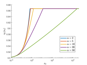
Figure 1: Solution of the infimal convolution problem (24) for $D_{f_{\alpha}}^{\Gamma}(Q\|P)$, where $\Gamma=\text{Lip}_{b}^{1}(\mathbb{R})$ and $Q$ and $P$ are given by Eq. (40). The left panel shows the mass $\eta_{*}(x_{2})$ as a function of $x_{2}$. For each value of $\alpha$ there is a transition point where all of the mass required by $Q$ at $x_{3}$ is first redistributed to $x_{2}$ when forming $\eta_{*}$, resulting in $\eta_{*}(x_{2})=2/3$. Note that the amount of mass moved to $x_{2}$ in the redistribution step does not depend on the distance of $x_{3}$ from $x_{2}$, only on the distance of $x_{2}$ from $x_{1}=0$. The right panel shows $D_{f_{2}}^{\Gamma}(Q\|P)$ as a function of $x_{2}$ and for several different values of the ratio $x_{3}/x_{2}$.

(see Eq. (97)); Eq. (41) is a simplification of Assumption 2 from Theorem 3.3 and (42) corresponds to Assumption 3. The solution to the infimal convolution problem then has the form

$$d\eta_{*}=\frac{1}{2}(f_{\alpha}^{*})^{\prime}(g_{*}(x_{1})-\nu_{*})\delta_{x_{1}}+\frac{1}{2}(f_{\alpha}^{*})^{\prime}(g_{*}(x_{2})-\nu_{*})\delta_{x_{2}}\,.$$ (44)

We will now outline how one solves for $\nu_{*}$ and $g_{*}$. Without loss of generality we can assume $g_{*}(x_{1})=0$ (the objective functional for $W^{\Gamma}$ is invariant under constant shifts and at the same time, shifting $g_{*}$ in $\eta_{*}$ can be achieved by redefining $\nu_{*}$). The only dependence on $g(x_{3})$ in Eq. (42) is in the $g(x_{3})/3$ term, hence the optimal solution has $g(x_{3})=x_{3}-x_{2}+g(x_{2})$. Therefore we need to solve

$$\frac{1}{2}(f_{\alpha}^{*})^{\prime}(-\nu_{*})+\frac{1}{2}(f_{\alpha}^{*})^{\prime}(g_{*}(x_{2})-\nu_{*})=1\,,$$ (45)

$$g_{*}(x_{2})\in\operatorname*{argmax}_{g(x_{2})\in[-x_{2},x_{2}]}\left\{\frac{1}{3}(x_{3}-x_{2})+\left(\frac{2}{3}-\frac{1}{2}(f^{*}_{\alpha})^{\prime}(g_{*}(x_{2})-\nu_{*})\right)g(x_{2})\right\}$$

for $\nu_{*}$ and $g_{*}(x_{2})$. The solution to this is obtained as follows:

1. Let $\nu_{*}(g_{2})$ be the unique solution to $\frac{1}{2}(f_{\alpha}^{*})^{\prime}(-\nu_{*})+\frac{1}{2}(f_{\alpha}^{*})^{\prime}(g_{2}-\nu_{*})=1$; the two terms on the left hand side will be used to obtain the redistributed weights in $\eta_{*}$.

2. Take $g_{*,2}$ such that $\frac{1}{2}(f_{\alpha}^{*})^{\prime}(g_{*,2}-\nu_{*}(g_{*,2}))=2/3$; this is inspired by the second line in Eq. (45).

3. If $0<x_{2}<g_{*,2}$ then the solution to Eq. (45) is obtained at $\nu_{*}=\nu_{*}(x_{2})$ and

   $$g_{*}(x)=\begin{cases}0,&x<0\\ x,&x\in[0,x_{3})\\ x_{3},&x\geq x_{3}\,.\end{cases}$$ (46)

   In this case, the optimal solution has $1/3<\eta_{*}(x_{2})<2/3$, i.e., some amount of mass is redistributed from $x_{1}=0$ to $x_{2}$ when forming $\eta_{*}$ and then mass is transported from both $x_{1}$ and $x_{2}$ to $x_{3}$ to form $Q$.

4. If $x_{2}\geq g_{*,2}$ then the solution to Eq. (45) is obtained at $\nu_{*}=\nu_{*}(g_{*,2})$ and

   $$g_{*}(x)=\begin{cases}0,&x<0\\ \frac{g_{*,2}}{x_{2}}x,&x\in[0,x_{2})\\ x-x_{2}+g_{*,2},&x\in[x_{2},x_{3})\\ x_{3}-x_{2}+g_{*,2},&x\geq x_{3}\,.\end{cases}$$ (47)

   In this case, $x_{2}$ is sufficiently far away from $x_{1}=0$ that the optimal solution, $\eta_{*}$, is obtained by first redistributing mass from $x_{1}=0$ to $x_{2}$ so that $\eta_{*}(x_{1})=1/3$, $\eta_{*}(x_{2})=2/3$. In the second step, mass is transported solely from $x_{2}$ to $x_{3}$ in order to form $Q$.

This completes the construction of $\eta_{*}$ from Eq. (44). The value of the $(f_{\alpha},\text{Lip}_{b}^{1}(\mathbb{R}))$-divergence can then be computed via Eq. (39). The computation of $g_{*,2}$ and $\nu_{*}(g_{*,2})$ from steps 1 and 2 must be done numerically and so we illustrate the solution graphically in Figure 1 by plotting $\eta_{*}(x_{2})$ as a function of $x_{2}$ for a number of $\alpha$’s. This shows how the mass must be redistributed when forming $\eta_{*}$ from $P$. The above calculations reveal an interesting transition; when $x_{2}$ is not close to $x_{1}$ then the mass is transferred solely from $x_{2}$ after it has been redistributed from $x_{1}$. However, when $x_{1}$ and $x_{2}$ are close enough then redistributing all the necessary mass from $x_{1}$ to $x_{2}$ is not optimal and it is cheaper to transport probability mass from both $x_{1}$ and $x_{2}$ to $x_{3}$. The transition between these cases corresponds to the point where $x_{2}$ crosses above $g_{*,2}$ (which depends on $\alpha$) and hence $\eta_{*}(x_{2})$ saturates at the value $2/3$.

4 Soft Constraints and the Divergence Property

For computational purposes, it is often advantageous to replace the hard (i.e., strict) constraint $g\in\Gamma$ with a soft constraint in the form of a penalty term, $V$, subtracted from the objective functional; by a penalty term, we mean $V$ ‘activates’ (i.e., is nonzero) when the constraint $g\in\Gamma$ is violated. In this way we can construct a new divergence $D_{f}^{V}$ with $D_{f}^{\Gamma}\leq D_{f}^{V}\leq D_{f}$ (we let the context distinguish between cases where the superscript denotes a constraint space and cases where it denotes a penalty term); see Theorem 4.4 for the main result of this section.

Of particular interest is the case $\Gamma=\text{Lip}^{1}_{b}(\mathbb{R}^{n})$ (we equip $\mathbb{R}^{n}$ with the Euclidean metric), where the $1$-Lipschtiz constraint can be relaxed to a one-sided gradient penalty term, thus defining objects such as

$$D_{f}^{\rho}(Q\|P)=\sup_{g\in\text{Lip}_{b}(\mathbb{R}^{n})}\left\{E_{Q}[g]-\Lambda_{f}^{P}[g]-\lambda\int\max\{0,\|\nabla g\|^{2}-1\}d\rho_{Q,P}\right\}\,,$$ (48)

where $\lambda>0$ is the strength of the penalty term and $\rho_{Q,P}$ is a positive measure (often depending on $Q$ and $P$). Here we are relying on Rademacher’s theorem (see Theorem 5.8.6 in [53]): $L$-Lipschitz functions on $\mathbb{R}^{n}$ are differentiable Lebesgue-a.e. and the norm of the gradient is bounded by $L$. The penalty term in Eq. (48) will therefore be activated only when $g$ is not $1$-Lipschitz.

Divergences with soft Lipschitz constraints were first applied to Wasserstein GAN [16] with great success, but the theoretical properties of such objects have not been explored; specifically, it has not been shown that they satisfy the divergence property. Here we show in great generality that the relaxation of a hard constraint to a soft constraint preserves the divergence property, and therefore objects such as (48) still provide a well-defined notion of ‘distance’ between probability measures. The basic requirement is that the penalty term, which we denote by $V$, vanishes on the constraint space $\Gamma$.

Lemma 4.1.

Let $(\Omega,\mathcal{M})$ be a measurable space, $\Gamma\subset\widetilde{\Gamma}\subset\mathcal{M}(\Omega)$, $H:\widetilde{\Gamma}\times\mathcal{P}(\Omega)\times\mathcal{P}(\Omega)\to\overline{\mathbb{R}}$, and $V:\widetilde{\Gamma}\times\mathcal{P}(\Omega)\times\mathcal{P}(\Omega)\to[0,\infty]$ with $V|_{\Gamma\times\mathcal{P}(\Omega)\times\mathcal{P}(\Omega)}=0$. Define

$$D^{\Gamma}(Q\|P)=\sup_{g\in\Gamma}H[g;Q,P]\,,\,\,\,\,\,D^{\widetilde{\Gamma}}(Q\|P)=\sup_{g\in{\widetilde{\Gamma}}}H[g;Q,P]\,,$$ (49)

$$D^{V}(Q\|P)=\sup_{g\in{\widetilde{\Gamma}}}\{H[g;Q,P]-V[g;Q,P]\}\,,$$

where $\infty-\infty\equiv-\infty$. If $D^{\Gamma}$ and $D^{\widetilde{\Gamma}}$ both have the divergence property then so does $D^{V}$.

Remark 4.2.

The convention $\infty-\infty\equiv-\infty$ is simply a convenient rigorous shorthand for restricting the supremum to those $g$’s for which this generally undefined operation does not occur.

Remark 4.3.

More generally, if the supremum $\sup_{g\in\Gamma}H[g;Q,P]$ is achieved at $g_{*}\in\Gamma$ (depending on $Q,P$) then the requirement $V|_{\Gamma\times\mathcal{P}(\Omega)\times\mathcal{P}(\Omega)}=0$ can be relaxed to $V[g_{*};Q,P]=0$ for all $Q,P$.

Proof.

Using $\Gamma\subset{\widetilde{\Gamma}}$, $V\geq 0$, and $V|_{\Gamma}=0$ we have $D^{\Gamma}\leq D^{V}\leq D^{\widetilde{\Gamma}}$. $D^{\Gamma}$ satisfies the divergence property, hence is non-negative. Therefore $D^{V}\geq 0$. $D^{\widetilde{\Gamma}}$ has the divergence property, hence if $Q=P$ then $0=D^{\widetilde{\Gamma}}(Q\|P)\geq D^{V}(Q\|P)\geq 0$. Therefore $D^{V}(Q\|P)=0$. Finally, if $D^{V}(Q\|P)=0$ then $D^{\Gamma}(Q\|P)=0$ and hence the divergence property for $D^{\Gamma}$ implies $Q=P$. ∎

Using Theorem 2.15 and Corollary B.19, we can apply Lemma 4.1 to the $(f,\Gamma)$-divergences and thereby conclude the following:

Theorem 4.4.

Let $f$ and $\Gamma\subset C_{b}(S)$ be strictly admissible. Let $\Gamma\subset{\widetilde{\Gamma}}\subset\mathcal{M}(S)$ and $V:{\widetilde{\Gamma}}\times\mathcal{P}(S)\times\mathcal{P}(S)\to[0,\infty]$ with $V|_{\Gamma\times\mathcal{P}(S)\times\mathcal{P}(S)}=0$. For $Q,P\in\mathcal{P}(S)$ define

$$D^{V}_{f}(Q\|P)\equiv\sup_{g\in{\widetilde{\Gamma}}}\left\{\left(E_{Q}[g]-\Lambda_{f}^{P}[g]\right)-V[g;Q,P]\right\}\,,$$ (50)

where $\infty-\infty\equiv-\infty$, $-\infty+\infty\equiv-\infty$. Then $D^{V}_{f}$ has the divergence property and $D_{f}^{\Gamma}\leq D_{f}^{V}\leq D_{f}$.

Proof.

Combine Lemma 4.1 with Part 4 of Theorem 2.15 and Theorem B.16 below; the latter shows that the variational formula for $D_{f}$ also holds when using the test-function space $\mathcal{M}(\Omega)$. ∎

4.1 Soft-Lipschitz Constraints on $\mathbb{R}^{n}$: One-Sided Versus Two-Sided Penalties

The gradient penalty term in Eq. (48) is one-sided, meaning that it penalizes $\|\nabla g\|>1$ but not $\|\nabla g\|\leq 1$. This is consistent with the hard constraint that the Lipschitz constant be less than or equal to $1$. The first use of soft Lipschitz penalties in [16], which considered the Wasserstein metric, also used a two-sided gradient penalty,

$$W^{\rho}(Q,P)=\sup_{g\in\text{Lip}_{b}(\mathbb{R}^{n})}\left\{E_{Q}[g]-E_{P}[g]-\lambda\int(\|\nabla g\|-1)^{2}d\rho_{Q,P}\right\}\,,$$ (51)

which penalizes $\|\nabla g\|\neq 1$. An intuitively reasonable requirement to impose on any soft constraint is that it vanish on the exact optimizer (if one exists) of the original strictly-constrained optimization problem. The justification for a two-sided gradient penalty in the Wasserstein case rests on Proposition 1 in [16], which shows that the exact optimizer of the Kantorovich-Rubinstein variational formula for the classical Wasserstein metric has gradient with norm $1$ a.e. As the two-sided gradient penalty vanishes on such functions, the object (51) will still possess the divergence property (see Remark 4.3). However, two-sided gradient penalties are not appropriate constraint-relaxations of the $(f,\Gamma)$-divergences, as the gradient of the exact optimizer generally does not have norm $1$ a.e. We demonstrate this via the following simple counterexample: Let $\Gamma=\text{Lip}^{1}_{b}(\mathbb{R}^{n})$, $P\in\mathcal{P}(\mathbb{R}^{n})$, and define $Q$ by $dQ/dP=Z^{-1}e^{-\min\{\|x\|,1\}/2}$. The optimizer of the variational formula defined in (14) is given for the classical KL divergence by

$$g_{*}=\log(dQ/dP)+1=-\min\{\|x\|,1\}/2+1+\log(Z^{-1})\,,$$ (52)

which is bounded and $1/2$-Lipschitz, and so $g_{*}\in\Gamma$. Therefore it is straightforward to see that $g_{*}$ is also the optimizer for $R^{\Gamma}(Q\|P)$ and it satisfies $\|\nabla g_{*}\|\leq 1/2$ a.e. This proves that the 2-sided penalty does not vanish on $g_{*}$. Similar counterexamples can be constructed using Eq. (14) for other choices of $f$.

5 Extension of the $(f,\Gamma)$-Divergence Variational Formula to Unbounded Functions

The assumption that all of the test functions $g\in\Gamma$ are bounded can be very restrictive in practice. In this section we provide general conditions under which the test-function space can be expanded to include (possibly) unbounded functions without changing the value of $D_{f}^{\Gamma}$. This fact will be used in the numerical examples in Section 6 below. The main result in this Section in Theorem 5.5.

The key step in the extension to unbounded $g$’s is the following lower bound.

Lemma 5.1.

Let $f$, $\Gamma$ be admissible and, in addition, suppose $f^{*}$ is bounded below. Fix $Q,P\in\mathcal{P}(S)$. If $g\in L^{1}(Q)$ and there exists $g_{n}\in\Gamma$, a measurable set $A$, and $C\in\mathbb{R}$ with $g_{n}\to g$ pointwise, $|g_{n}|\leq|g|$ for all $n$, and $g_{n}\leq g1_{A}+C1_{A^{c}}$ for all $n$, then

$$D_{f}^{\Gamma}(Q\|P)\geq E_{Q}[g]-\Lambda_{f}^{P}[g]\,.$$ (53)

Remark 5.2.

The additional assumption that $f^{*}$ is bounded below is satisfied in many cases of interest, e.g., the KL divergence and $\alpha$-divergences for $\alpha>1$.

Proof.

We need to show that

$$D_{f}^{\Gamma}(Q\|P)\geq E_{Q}[g]-(\nu+E_{P}[f^{*}(g-\nu)])$$ (54)

for all $\nu\in\mathbb{R}$. Note that we have assumed $f^{*}$ is bounded below by some $D\in\mathbb{R}$, hence $E_{P}[f^{*}(g-\nu)]$ exists in $(-\infty,\infty]$. If $E_{P}[f^{*}(g-\nu)]=\infty$ then the claim is trivial, so for the remainder of this proof we suppose $f^{*}(g-\nu)\in L^{1}(P)$.

The assumptions on $g$ allow us to use the dominated convergence theorem to conclude $E_{Q}[g_{n}]\to E_{Q}[g]$. Continuity of $f^{*}$ implies $f^{*}(g_{n}-\nu)\to f^{*}(g-\nu)$. The admissibility assumption implies $\lim_{y\to-\infty}f^{*}(y)<\infty$. Using this together with Lemma A.4 we see that $f^{*}$ is nondecreasing, hence

$$D\leq f^{*}(g_{n}-\nu)\leq f^{*}(g-\nu)1_{A}+f^{*}(C-\nu)1_{A^{c}}\in L^{1}(P)\,.$$ (55)

Therefore the dominated convergence theorem implies $E_{P}[f^{*}(g_{n}-\nu)]\to E_{P}[f^{*}(g-\nu)]$. We have $g_{n}\in\Gamma$, hence Eq. (15) implies

$$D_{f}^{\Gamma}(Q\|P)\geq \lim_{n\to\infty}\left(E_{Q}[g_{n}]-(\nu+E_{P}[f^{*}(g_{n}-\nu)])\right)$$ (56)

$$= E_{Q}[g]-(\nu+E_{P}[f^{*}(g-\nu)])\,.$$

This completes the proof. ∎

Using Lemma 5.1, one can augment $\Gamma$ by including any functions that satisfy the stated assumptions; this will not change the value of the supremum in (15). Rather than formulating a general result of this type, we consider one of the most useful special cases, the set of Lipschitz functions. Other cases can be treated similarly.

Lemma 5.3.

Let $c:S\times S\to[0,\infty]$, $L\in(0,\infty)$, and define

$$\text{Lip}_{b}^{L}(S,c)=\{g\in C_{b}(S):|g(x)-g(y)|\leq Lc(x,y)\text{ for all }x,y\in S\}\,.$$ (57)

If $c=d$ (the metric on $S$) then we use our earlier notation, $\text{Lip}_{b}^{L}(S)$, in place of $\text{Lip}_{b}^{L}(S,d)$.

The set $\text{Lip}_{b}^{L}(S,c)$ is admissible and if $d\leq Kc$ for some $K\in(0,\infty)$ then $\text{Lip}_{b}^{L}(S,c)$ is strictly admissible.

Proof.

Convexity is trivial. Weak convergence in $C_{b}(S)$ implies pointwise convergence (take $\mu=\delta_{x}$, $x\in S$), hence $\text{Lip}_{b}^{L}(S,c)$ is closed. Finally, if $d\leq Kc$ then strict admissibility follows from the fact that $\text{Lip}_{b}^{L/K}(S)$ is $\mathcal{P}(S)$-determining and $\text{Lip}_{b}^{L/K}(S)\subset\text{Lip}_{b}^{L}(S,c)$. ∎

Remark 5.4.

For $L>0$ we have $\text{Lip}^{L}_{b}(S,c)=\{Lg:g\in\text{Lip}^{1}_{b}(S,c)\}$ and so (under appropriate assumptions) Theorem 2.17 implies the following limiting formulas:

$$\lim_{L\to\infty}D_{f}^{\text{Lip}^{L}_{b}(S,c)}(Q\|P)=D_{f}(Q\|P)\,,$$ (58)

$$\lim_{L\searrow 0}L^{-1}D_{f}^{\text{Lip}^{L}_{b}(S,c)}(Q\|P)=W^{\text{Lip}^{1}_{b}(S,c)}(Q,P)\,.$$

Using Lemma 5.1 we can show that the boundedness constraint can be dropped in the formula for $D_{f}^{\Gamma}$ when $\Gamma=\text{Lip}_{b}^{L}(S,c)$; we exploit this fact in the numerical examples in Section 6 below.

Theorem 5.5.

Let $c:S\times S\to[0,\infty]$, $L\in(0,\infty)$, and define

$$\text{Lip}^{L}(S,c)=\{g\in C(S):|g(x)-g(y)|\leq Lc(x,y)\text{ for all }x,y\in S\}\,.$$ (59)

Let $f$ be admissible such that $f^{*}$ is bounded below. Then for $Q,P\in\mathcal{P}(S)$ we have

$$D_{f}^{\text{Lip}_{b}^{L}(S,c)}(Q\|P)= \sup_{g\in\text{Lip}^{L}(S,c)\cap L^{1}(Q)}\left\{E_{Q}[g]-\Lambda_{f}^{P}[g]\right\}\,.$$ (60)

Proof.

Lemma 5.3 shows that $\Gamma\equiv\text{Lip}_{b}^{L}(S,c)$ satisfies the conditions of Theorem 2.15. Fix $g\in\text{Lip}^{L}(S,c)\cap L^{1}(Q)$. For $n\in\mathbb{Z}^{+}$ define $g_{n}=n1_{g>n}+g1_{-n\leq g\leq n}-n1_{g<-n}$. It is easy to see that $g_{n}\in\text{Lip}_{b}^{L}(S,c)$, $g_{n}\to g$, $|g_{n}|\leq|g|$, $g_{n}\leq g1_{g\geq 0}$. Therefore Lemma 5.1 implies

$$D_{f}^{\Gamma}(Q\|P)\geq E_{Q}[g]-\inf_{\nu\in\mathbb{R}}\{\nu+E_{P}[f^{*}(g-\nu)]\}\,.$$ (61)

One inequality in Eq. (60) follows from taking the supremum over all $g\in\text{Lip}^{L}(S,c)\cap L^{1}(Q)$ in Eq. (61) and the reverse follows from the fact that $\text{Lip}_{b}^{L}(S,c)\subset\text{Lip}^{L}(S,c)\cap L^{1}(Q)$. ∎

6 $(f,\Gamma)$-GANs

Generative adversarial networks constitute a class of methods for ‘learning’ a probability distribution, $Q$, via a two-player game between a discriminator and a generator (both neural networks) [13, 15, 14, 16, 54]. Mathematically, most GANs can be formulated as divergence minimization problems for a divergence, $D$, that has a variational characterization $D(Q\|P)=\sup_{g\in\Gamma}H[g;Q,P]$. The goal is then to solve the following optimization problem:

$$\inf_{\theta\in\Theta}D(Q\|P_{\theta})=\inf_{\theta\in\Theta}\sup_{g\in\Gamma}H[g;Q,P_{\theta}] \,.$$ (62)

Here, $g$ is called the discriminator and $P_{\theta}$ is the distribution of $h_{\theta}(X)$, where $X$ is a random noise source and $h_{\theta}$, $\theta\in\Theta$ is a neural network family (the generator). The minimax problem (62) can be interpreted as two-player zero-sum game. GANs based on the Wasserstein-metric have been very successful [14, 16] and GANs based on the classical $f$-divergences have also been explored [15]. Here we show that GANs based on the $D_{f}^{\Gamma}$ divergences, which generalize and interpolate between the above two extremes, inherit desirable properties from both IPM-GANs (e.g., Wasserstein GAN) and $f$-GANs. Specifically, we focus on the following:

1. $(f,\Gamma)$-GANs can perform well when applied to heavy-tailed distributions. This property is inherited from the classical $f$-divergences.

2. $(f,\Gamma)$-GANs can perform well even when there is a lack of absolute continuity. This property is inherited from the $\Gamma$-IPMs.

We will specifically focus on the cases where $f=f_{\alpha}$, $\alpha>1$, (see Eq. (8)) and $\Gamma=\text{Lip}_{b}^{L}(\mathbb{R}^{n})$ (see Lemma 5.3). We call the corresponding $(f,\Gamma)$-divergences the Lipschitz $\alpha$-divergences and will denote them by $D_{\alpha}^{L}$. As $\Gamma$ is closed under shifts, we can express these divergences in one of two ways (see Eq. (18)):

$$D^{L}_{\alpha}(Q\|P)= \sup_{g\in\text{Lip}_{b}^{L}(\mathbb{R}^{n})}\{E_{Q}[g]-\Lambda_{f_{\alpha}}^{P}[g]\}$$ (63)

$$= \sup_{g\in\text{Lip}_{b}^{L}(\mathbb{R}^{n})}\{E_{Q}[g]-E_{P}[f_{\alpha}^{*}(g)]\}\,.$$ (64)

The formula for $f_{\alpha}^{*}$ can be found in Eq. (97) below.

Remark 6.1.

Formally taking the $\alpha\to\infty$ limit of (64) we arrive at what we call the Lipschitz $\infty$-divergence:

$$D^{L}_{\infty}(Q\|P)= \sup_{g\in\text{Lip}_{b}^{L}(\mathbb{R}^{n})}\{E_{Q}[g]-E_{P}[\max\{g,0\}]\}\,.$$ (65)

It is straightforward to show that $D^{L}_{\infty}(Q\|P)=LW(Q,P)$, where $W$ is classical Wasserstein metric

$$W(Q,P)=\sup_{g\in\text{Lip}_{b}^{1}(\mathbb{R}^{n})}\{E_{Q}[g]-E_{P}[g]\}\,,$$ (66)

though they are expressed in terms of different objective functionals (hence their performance can differ in practice).

In numerical computations it can be inconvenient to restrict one’s attention to bounded discriminators only. Fortunately, as shown in Theorem 5.5 above, the equality (15) remains true when $\Gamma$ is expanded to include many unbounded $g$’s. This fact justifies our use of unbounded discriminators (i.e., unbounded activation functions) in the following computations.

As our baseline method we take the two-sided gradient-penalized Wasserstein GAN (WGAN-GP) from [16]:

WGAN-GP:

$$\inf_{\theta}\sup_{g\in\text{Lip}(\mathbb{R}^{n})}\left\{E_{Q}[g]-E_{P_{\theta}}[g]-\lambda\int(\|\nabla g\|/L-1)^{2}d\rho_{\theta}\right\}\,,$$ (67)

where $\lambda>0$ is the strength of the penalty regularization. Here, and below, we have relaxed the Lipschitz constraint to a gradient penalty (two-sided for WGAN-GP and one-sided otherwise; see Section 4 for further discussion). We approximate the supreumum over $g$ by the supremum over a neural network family (the discriminator network). Again, the family of measures $P_{\theta}$ are the distributions of $X_{\theta}=h_{\theta}(X)$ where $h_{\theta}$ is the generator neural network, parameterized by $\theta\in\Theta$, and we let $X$ be a Gaussian noise source. Finally, we let $\rho_{\theta}\sim TX_{\theta}+(1-T)Y$ where $X_{\theta}$, $Y\sim Q$, $T\sim Unif([0,1])$ are all independent (this choice of $\rho_{\theta}$ was used in [16]).

We compare WGAN-GP to the Lipschitz $\alpha$-GANs and Lipschitz KL-GAN, defined based on (64) and (63) respectively:

Lipschitz $\alpha$-GAN

$$\inf_{\theta\in\Theta}\sup_{g\in\text{Lip}(\mathbb{R}^{n})}\left\{E_{Q}[g]-E_{P_{\theta}}[f_{\alpha}^{*}(g)]-\lambda\int\max\{0,\|\nabla g\|^{2}/L^{2}-1\}d\rho_{\theta}\right\}\,.$$ (68)

When we want to make the values of $\alpha$ and/or $L$ explicit we will refer to these as the $D_{\alpha}^{L}$-GANs. By swapping $Q$ and $P_{\theta}$ one obtains another family of GANs, which we call the reverse Lipschitz $\alpha$-GANs (when clarity is needed, (68) will be called a forward GAN). We note that forward and reverse GANs can have very different properties [55].

In the case of the KL-divergence one can evaluate the optimization over $\nu$ in (63) (see Eq. (19)), leading to the following:

Lipschitz KL-GAN

$$\inf_{\theta\in\Theta}\sup_{g\in\text{Lip}(\mathbb{R}^{n})}\left\{E_{Q}[g]-\log E_{P_{\theta}}[e^{g}]-\lambda\int\max\{0,\|\nabla g\|^{2}/L^{2}-1\}d\rho_{\theta}\right\}\,.$$ (69)

Remark 6.2.

For numerical purposes the GAN (69), obtained using the representation (11), performs significantly better than the GAN obtained from (10). This is due to the numerical issues inherent in computing $E_{P}[f^{*}_{KL}(g)]=E_{P}[\exp(g-1)]$, as compared to computing the cumulant generating function $\log E_{P}[\exp(g)]$; see also [11]. We also refer to [26] for a more general perspective on finding tighter variational representations of divergences.

6.1 Statistical Estimation of $(f,\Gamma)$-Divergences

In numerical computations, we approximate the $(f,\Gamma)$-divergence by replacing expectations under $Q$ and $P$ in (15) or (17) with their $m$-sample empirical means using i.i.d. samples from $Q$ and $P$ respectively, i.e., we estimate

$$E[D_{f}^{\Gamma}(Q_{m}\|P_{m})]=E\left[\sup_{g\in\Gamma,\nu\in\mathbb{R}}\{E_{Q_{m}}[g-\nu]-E_{P_{m}}[f^{*}(g-\nu)]\}\right]\,.$$ (70)

Note that, at fixed $g$ and $\nu$, the objective functional on the right-hand-side of (70) is an unbiased estimator of the $(f,\Gamma)$-divergence objective functional. Including the optimization over $g$ and $\nu$ we obtain a biased estimator which is an upper bound on $D_{f}^{\Gamma}$, as shown in the lemma below.

Lemma 6.3.

Let $f\in\mathcal{F}_{1}(a,b)$, $\Gamma\subset\mathcal{M}_{b}(\Omega)$ be nonempty, $Q,P\in\mathcal{P}(\Omega)$, and $Q_{m}$, $P_{m}$ be empirical distributions constructed from $m$ i.i.d. samples from $Q$ and $P$ respectively. Then

$$E[D_{f}^{\Gamma}(Q_{m}\|P_{m})]\geq D_{f}^{\Gamma}(Q\|P)\,.$$ (71)

Proof.

Using (17) we can compute

$$E[D_{f}^{\Gamma}(Q_{m}\|P_{m})]= E\left[\sup_{g\in\Gamma,\nu\in\mathbb{R}}\{E_{Q_{m}}[g-\nu]-E_{P_{m}}[f^{*}(g-\nu)]\}\right]$$ (72)

$$\geq \sup_{g\in\Gamma,\nu\in\mathbb{R}}E\left[E_{Q_{m}}[g-\nu]-E_{P_{m}}[f^{*}(g-\nu)]\right]$$

$$= \sup_{g\in\Gamma,\nu\in\mathbb{R}}\{E_{Q}[g-\nu]-E_{P}[f^{*}(g-\nu)]\}=D_{f}^{\Gamma}(Q\|P)\,.$$

∎

Remark 6.4.

As noted above, in the KL case one can evaluate the optimization over $\nu$ in (70). This results in a biased objective functional due to the presence of the logarithm outside the expectation in (19). This same issue was addressed earlier in [11], e.g., by using sufficiently large minibatch sizes or an exponential moving average. This concern is not present in the objective functional for (70) (or (68)).

In the following GAN examples we work with Lipschitz functions and approximate the optimization over $\text{Lip}(\mathbb{R}^{n})$ by the optimization over some neural network family $g_{\phi}$, $\phi\in\Phi$, and estimate the expectations using the $m$-sample empirical measures $Q_{m}$, $P_{m,\theta}$, $\rho_{m,\theta}$, e.g., we approximate the Lipschitz $\alpha$-GAN (68) by

$$\inf_{\theta\in\Theta}\sup_{\phi\in\Phi}\left\{E_{Q_{m}}[g_{\phi}]-E_{P_{m,\theta}}[f_{\alpha}^{*}(g_{\phi})]-\lambda\int\max\{0,\|\nabla g_{\phi}\|^{2}/L^{2}-1\}d\rho_{m,\theta}\right\}\,.$$ (73)

Various neural network architectures are known to be universal approximators [56, 50, 57, 58, 59]. Approximating the supremum over $g\in\text{Lip}(\mathbb{R}^{n})$ by the supremum over a finite-dimensional neural network family essentially results in a lower bound on the original, intended divergence. In the case of KL and Rényi divergences, such an approximation scheme is known to lead to consistent estimators as the sample size and network complexity grows (see [11] and [60] respectively). Investigating the analogous consistency result for the $(f,\Gamma)$-divergence estimator is one avenue for future work.

6.2 $(f,\Gamma)$-GANs for Non-Absolutely-Continuous Heavy-Tailed Distributions

We mentioned above that the $f$-divergences are better suited to heavy-tailed distributions, as compared to the Wasserstein metric. Before demonstrating this in the context of GANs we provide a simple explicit example. Let $dQ=x^{-2}1_{x\geq 1}dx$ and $dP=(1+\delta)x^{-(2+\delta)}1_{x\geq 1}dx$ for $\delta>0$, i.e., the tail of $P$ decays faster than that of $Q$. For $\alpha>1$ we can use Eq. (7) to compute

$$D_{f_{\alpha}}(Q\|P)=\frac{1}{\alpha(\alpha-1)(1+\delta)^{\alpha-1}}\int_{1}^{\infty}x^{\delta\alpha-(2+\delta)}dx-\frac{1}{\alpha(\alpha-1)}\,,$$ (74)

and so $D_{f_{\alpha}}(Q\|P)<\infty$ for all $\delta\in(0,1/(\alpha-1))$. On the other hand, we can use the formula for the Wasserstein metric on $\mathcal{P}(\mathbb{R})$ from [61] to compute

$$W(Q,P)= \int_{-\infty}^{\infty}|F_{Q}(t)-F_{P}(t)|dt=\int_{1}^{\infty}t^{-1}-t^{-(1+\delta)}dt=\infty$$ (75)

for all $\delta>0$ ($F_{P}$ and $F_{Q}$ denote the cumulative distribution functions).

This calculation suggests that Lipschtiz $\alpha$-GANs may succeed for heavy-tailed distributions, even when WGAN-GP fails to converge. On the other hand the Wasserstein metric can be finite and informative even when $Q$ and $P$ are non-absolutely continuous, unlike the classical $f$-divergences (7). The $(f,\Gamma)$-divergences inherit both of these strengths from the Wasserstein and $f$-divergences (see Part 1 of Theorem 2.15), thus allowing for the training of GANs with heavy-tailed data and in the absence of absolute continuity. We demonstrate this via the following example, where both the WGAN-GP and classical $f$-GAN (i.e., without gradient penalty) fail to converge but the $(f,\Gamma)$-GANs succeed.

Here the data source, $Q$, is a mixture of four 2-dimensional t-distributions with $0.5$ degrees of freedom, embedded in a plane in 12-dimensional space; note that this is a heavy-tailed distribution, as the mean does not exist; this suggests that WGAN will have difficulty learning this distribution. The generator uses a 10-dimensional noise source and so the generator and data source are generally not absolutely continuous with respect to one another (the former has support equal to the full 12-dimensional space while the latter is supported on a 2-dimensional plane). This suggests one cannot use the classical $f$-GAN [15], i.e., without gradient penalty (we confirmed that they perform very poorly on this problem). The $(f,\Gamma)$-GANs allow us to address both of the above difficulties; heavy tails can be accommodated by an appropriate choice of $f$ and the lack of absolute continuity is addressed by using a $1$-Lipschitz constraint (as in the Wasserstein metric).

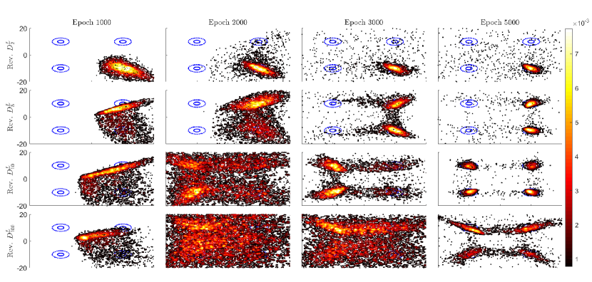
(a)

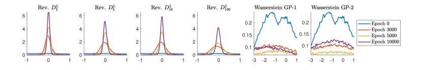
(b)

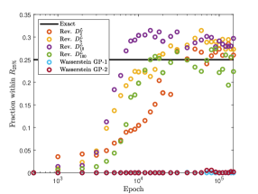
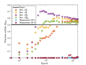
(c)

Figure 2: We present generator samples and their statistical behavior from Wasserstein and reverse Lipschitz $\alpha$-GAN methods. The dataset used in training consists of 5000 samples from a mixture of four 2-dimensional t-distributions with $0.5$ degrees of freedom that are embedded in a plane in 12-dimensional space. Panel (a) shows the projection onto the 2-dimensional support plane (each column shows the result after a given number of training epochs; the solid and dashed blue ovals mark the 25% and 50% probability regions, respectively, of the data source while the heat-map shows the generator samples. Panel (b) shows the generator distribution, projected onto components orthogonal to the support plane. Values concentrated around zero indicate convergence to the sub-manifold. In Panel (c) we show the fraction of generator samples, projected onto the 2D support plane of the measure, that are within the $25\%$ and $50\%$ probability regions. In this example we used gradient-penalty parameter values $\lambda=10$, $L=1$; Wasserstein GAN was run with both 1-sided and 2-sided gradient penalties (GP-1 and GP-2 respectively). In all cases the generator and discriminator have three fully connected hidden layers of 64, 32, and 16 nodes respectively, and with ReLU activation functions. The generator uses a 10-dimensional Gaussian noise source. Each SGD iteration was performed with a minibatch size of 1000 and 5 discriminator iterations were performed for every one generator iteration. Computations were done in TensorFlow and we used the RMSProp SGD algorithm with a learning rate of $2\times 10^{-4}$.

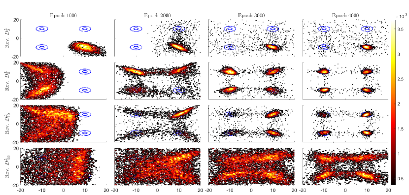
(a)

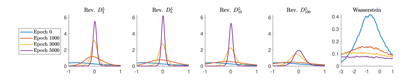
(b)

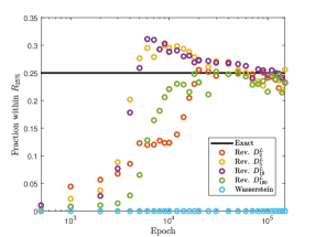
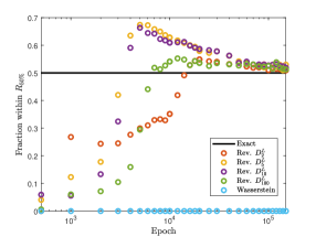
(c)

Figure 5: Here we present generator samples and their statistical behavior from Wasserstein and reverse Lipschitz $\alpha$-GAN methods using the same setup as in Figure 5, except that training was done with a much larger set of samples (100000 samples). We obtain similar results, with the primary difference being that the training converges faster.

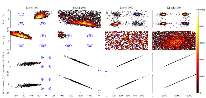
Figure 6: Here we present generator samples from WGAN-GP, reverse classical $f$-GAN (denoted $D_{\alpha}$), and reverse Lipschitz $\alpha$-GAN using the setup described in Section 6.2 and Figure 5, except that we do not embed in higher-dimensional space; the results are similar to what was described in Section 6.2. In the case of classical $f$-GAN this is intriguing since, unlike in Figure 5, here we have $D_{f}(P_{\theta}\|Q)<\infty$ yet the classical $f$-GAN still fails to converge. This suggests that the Lipschitz constraint aids in the stability of the training even in such cases where the classical $f$-divergence is finite. We show the result only for $\alpha=5$ but the behavior for other values of $\alpha$ is similar.

In Figure 2 below we show generator samples for Wasserstein GAN, as in Eq. (67) and [16], and for various reverse Lipschitz $\alpha$-GANs (68). Specifically, panel (a) shows the projection onto the 2-dimensional support plane of $Q$ (the heat-map shows samples from the generator and the data source, $Q$, is illustrated by the blue ovals) and panel (b) shows the generator distribution, projected onto components orthogonal to the support plane. Panel (a) does not show WGAN-GP samples, as WGAN-GP failed to converge in this example; this is demonstrated in panel (b) wherein we see that the Lipschitz $\alpha$-GAN samples concentrate near the support plane (at $0$) while the WGAN-GP samples spread out away from the support plane. The classical $f$-GAN without gradient penalty [15], which we don’t show here, similarly failed to converge; this is unsurprising due to the lack of absolute continuity. Again, we can see that WGAN-GP fails to converge, while the Lipschitz $\alpha$-GANs perform well. Some $\alpha$’s perform significantly better than others, making it an important hyperparameter to tune in this case. Results from a second set of runs, using a larger sample set, are shown in Figure 5 in Appendix E; the conclusions are similar. Forward Lipschitz GANs and forward Lipschitz KL-GANs all experienced blow-up and so they are not shown here. This behavior is reasonable when one considers the fact that $Q$ is heavy tailed, while $P_{\theta}$ is not (it is generated by pushing forward Gaussian noise by Lipschitz functions), and so $D_{f}(Q\|P_{\theta})=\infty$, while $D_{f}(P_{\theta}\|Q)<\infty$ (see Eq. (7)). As we have already demonstrated the inability of the Wasserstein metric to compare heavy-tailed distributions (see Eq. (75)), it is reasonable to conjecture that the finiteness of $D_{f_{\alpha}}$ is key in determining the success of the $D_{\alpha}^{L}$-GAN. Interestingly, the Lipschitz constraint also appears to be key to the convergence of the method, something one would not anticipate solely based on finiteness of the corresponding divergences. We illustrate this with Figure 6 in Appendix E, where we apply the same method to the mixture of four 2-dimensional t-distributions, but without the high-dimensional embedding. In this case, the classical $f$-divergence is finite, however we find that the classical $f$-GAN fails to converge –WGAN also fails– but the $(f,\Gamma)$-GANs succeed. The theoretical understanding of this behavior is an interesting question, but we will not pursue it further here.

6.3 Strict Convexity and Enhanced Stability of $(f,\Gamma)$-GANs

Even in the absence of heavy tails, we find that the Lipschitz $\alpha$-GANs can outperform WGAN-GP, as measured both by accuracy on quantities of interest as well as improved stability. The improved stability can be motivated by a simple (formal) calculation of the Hessian of the objective functional in Eq. (18),

$$H_{f}[g;Q,P]\equiv E_{Q}[g]-E_{P}[f^{*}(g)]$$ (76)

(see Appendix D for an analysis of the objective functional in the non shift-invariant case (15)). Let $g_{0}\in\Gamma$ and perturb in some direction $\psi$, i.e., take a line segment $g_{\epsilon}=g_{0}+\epsilon\psi\in\Gamma$. Then

$$\frac{d^{2}}{d\epsilon^{2}}|_{\epsilon=0}H_{f}[g_{\epsilon};Q,P]=-E_{P}[(f^{*})^{\prime\prime}(g_{0})\psi^{2}]\,.$$ (77)

Convexity of $f^{*}$ implies $(f^{*})^{\prime\prime}\geq 0$. If we have $(f^{*})^{\prime\prime}>0$ then (77) implies the objective functional is strictly concave at $g_{0}$ in all directions, $\psi$, are nonzero on a set of positive $P$-probability. This strict concavity implies that the maximization problem (15) is a strictly convex optimization problem and suggests that numerical computation of $D_{f}^{\Gamma}(Q\|P)$ via (15) may generally be more stable than computation of the $\Gamma$-IPM (16), as the latter uses a linear objective functional. Indeed, in [62] the authors demonstrated that gradient descent/ascent dynamics (used for training of GANs) oscillate without converging to the optimum for the Wasserstein-GAN loss function (16) in the special case where $\Gamma$ consists of a parametric family of linear functions. In this case, more sophisticated algorithms such as training with optimism [62] or two-step extra-gradient approaches [63] were required to guarantee convergence. Here our $(f,\Gamma)$ interpolation replaces the optimization of a linear objective functional in the case of the $\Gamma$-IPM (16) with the strictly concave problem (15). In the case of a linear discriminator space $\Gamma$, we obtain a complete theoretical justification based on the concavity calculation (77). In particular, we consider (76) where

$$H_{f}[g_{\phi};Q,P]=E_{Q}[g_{\phi}]-E_{P}[f^{*}(g_{\phi})]\,,$$ (78)

and where we assume that $\Gamma=\{g=g_{\phi}(x):\phi=(\phi_{1},\phi_{2},...,\phi_{k})\in D\}$ is a parametric linear family ($D$ is a closed, convex subset of $\mathbb{R}^{k}$), i.e., for any constants $a_{0},a_{1}$ and any parameter values $\phi_{0}$, $\phi_{1}$ we have

$$g_{a_{0}\phi_{0}+a_{1}\phi_{1}}(x)=a_{0}g_{\phi_{0}}(x)+a_{1}g_{\phi_{1}}(x)\,.$$ (79)

Using (79) and considering (77) for any $g=g_{\phi_{0}}$ and $\psi(x)=g_{\phi_{1}}$, $g_{\epsilon}=g_{\phi_{0}}+\epsilon g_{\phi_{1}}$, we readily have

$$\phi_{1}^{\intercal}\nabla_{\phi}^{2}H_{f}[g_{\phi_{0}};Q,P]\phi_{1}=\frac{d^{2}}{d\epsilon^{2}}|_{\epsilon=0}H_{f}[g_{\epsilon};Q,P]=-E_{P}[(f^{*})^{\prime\prime}(g_{\phi_{0}})g_{\phi_{1}}^{2}]\,,$$ (80)

provided all expected values are finite. As in (77), this analysis implies the strict concavity of (78) with respect to the linear parametrization $\phi$. Thus our analysis covers linear spaces $\Gamma$ such as linear combinations of splines or reproducing kernel Hilbert spaces (RKHS). However, when $\Gamma$ is a family of neural networks then the $g_{\phi}$’s are not linear in $\phi$ and the above analysis does not apply. We will not pursue the theoretical analysis of this important case here but instead we will carry out an empirical study that explores the improved stability that (local) strict concavity would imply.

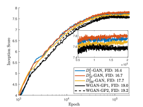
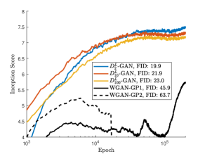
Figure 3: Comparison between Lipschitz $\alpha$-GAN and WGAN-GP (both 1 and 2-sided) on the CIFAR-10 dataset. Here we plot the inception score as a function of the number of training epochs (moving average over the last 5 data points, with results averaged over 5 runs). We also show the averaged final FID score in the legend, computed using 50000 samples from both $Q$ and $P$. The neural network architecture is as in Appendix F of [16]; in particular, it employs residual blocks. The left panel used an initial learning rate of $0.0002$ (the same as in [16]) while in the right panel we used an initial learning rate of $0.001$. Here, and in other similar tests, we find the Lipschitz $\alpha$-GANs to be significantly more stable and require less tuning of the learning rate; in particular, none of the WGAN-GP2 runs shown in the right panel were able to complete successfully.

In Figure 3 we demonstrate both improved performance and improved stability of the Lipschitz $\alpha$-GANs, as compared to WGAN-GP, on the CIFAR-10 dataset [41], which consists of 32x32 RGB images from 10 classes. We use the same ResNet neural network architecture as in [16, Appendix F] and focus on evaluating the benefits of simply modifying the objective functional. We employ the adaptive learning rate Adam Optimizer method [64] using the hyperparameter values shown in Algorithm 1 of [16] (note that in [16], $\alpha$ denotes the learning rate parameter and should not be confused with our use for $\alpha$-divergences). We show the inception score as a function of the number of training epochs; the inception score [39] is a commonly used performance measure for evaluating the diversity of images produced by a GAN. It uses a pre-trained classifier to estimate the number of distinct classes produced by the generator and so, when applied to CIFAR-10, values closer to 10 are considered better. In the legends we also show the final FID score achieved by each method. FID score is a performance measure that computes a distance between feature vectors of a classification model when applied to the original data, as compared to the generated samples [40]; a lower FID score is better. In the left panel of Figure 3 we show the results using an initial learning rate of $0.0002$; we find a small improvement in inception score and substantial improvement in FID score when using the Lipschitz $\alpha$-GANs, as compared to WGAN-GP (either $1$ or $2$-sided). In this example we find the performance to be relatively insensitive to the value of $\alpha$.

In addition to the performance improvement, we find the Lipschitz $\alpha$-GANs to be far less sensitive to the choice of learning rate. In the right panel of Figure 3 we show results using an initial learning rate of $0.001$; here we observe significant degradation of the performance of WGAN-GP, but only a slight impact on the Lipschitz $\alpha$-GANs. We conjecture that this increased stability is due to the strong concavity of the $(f,\Gamma)$-divergence objective functionals. Regarding increased stability, these numerical findings, the analysis for a general (non-parameterized) function space $\Gamma$ in (77), as well as for the linear parametric case (80) provide only preliminary indications for the conjecture; a dedicated analysis for general parameterized $\Gamma$’s that will include nonconvex parametric families such as neural networks is clearly necessary but we will not pursue it further here.

6.3.1 Enhanced Stability and Spectral Normalization

In [35] the authors showed that spectral normalization, which directly controls the Lipschitz constant of each layer of a neural network by setting the largest singular value of its weight matrix to $1$, provides enhanced stability as compared to WGAN-GP and at a lower computational cost (see Figures 1 and 2 in [35]). Their method, which uses the Jensen-Shannon divergence, is equivalent to Eq. (18) (i.e., they do not include an optimization over shifts as in (17)) with a change of variables $g=\log(D)$ and using a function space $\Gamma$ that consists of a neural network family with spectral normalization. In this example we use a spectral normalization function space in our method (17); this falls under the purview of Theorem 2.8 (see Table 2). We provide empirical evidence that the improved stability they observed is at least partially due to the strict concavity of the objective functional. Specifically, we find that WGAN with spectral normalization fails to inherit this improved stability and even fails to outperform WGAN-GP. Our results demonstrate that combining spectral normalization with other (strictly convex) objective functionals can enhance stability, similar both to what was observed in [35] and also to what we found in Figure 3. Here we again study the case $f=f_{\alpha}$, denoting these methods by $D_{\alpha}^{SN}$; results are shown in Figure 4.

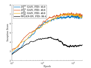
Figure 4: A comparison between Lipschitz $\alpha$-GAN and WGAN, both using spectral normalization (SN) to enforce Lipschitz constraints. We used an initial learning rate of $0.0001$ and otherwise employed same ResNet architecture and hyperparameters as in Figure 3. In particular, we did not attempt to further optimize the architecture when changing from a gradient penalty to SN. None of the methods performed as well as their gradient penalty counterparts from Figure 3, but note the especially poor performance of WGAN-SN. This suggests a further robustness of our methods to the use of sub-optimal architecture and hyperparameters.

7 Conclusion

We have provided a systematic and rigorous exploration of the properties of the $(f,\Gamma)$-divergences, as defined in Eq. (1). This work was motivated by the need for a flexible collection of novel divergences that combine key properties from $f$-divergences and Wasserstein metrics, such as the ability to work with heavy tails and with not-absolutely continuous distributions. A large list of proposed GANs fall under the presented mathematical framework (see Table 2), unifying to a considerable extent the loss formulation of GANs. We have illustrated the utility of the $(f,\Gamma)$-divergences in the training of GANs, showing both an increased domain of applicability and improved convergence stability. The theoretical results allow for a wide range of choices on $f$ and $\Gamma$. We have shown that there are families of distributions that are better suited for $(f,\Gamma)$-divergence over either $f$-divergence or $\Gamma$-IPM. A more systematic exploration on the selection of proper $f$ and $\Gamma$ will add practical value from a practitioner’s perspective, but further and more elaborate experimentation is required, along with a need for new theoretical insights. In the future we intend to further study the stability, the related statistical estimation theory, and explore these new divergences in additional challenging settings such as high-dimensional time-series generation, extreme events prediction, mutual information estimation, and uncertainty quantification for heavy-tailed distributions and in the absence of absolute continuity.

Appendix A Properties of the Legendre Transform of $f\in\mathcal{F}_{1}(a,b)$

Here we collect a number of important properties regarding the LT of function in $\mathcal{F}_{1}(a,b)$. Recall that we use the same notation for the convex LSC extension $f:\mathbb{R}\to(-\infty,\infty]$ (see Definition 2.2). First we state an important continuity result [46, Theorem 10.1].

Lemma A.1.

Let $f\in\mathcal{F}_{1}(a,b)$. Then $f^{*}(y)=\sup_{x\in(a,b)}\{yx-f(x)\}$ and $f^{*}$ is continuous on $\overline{\{f^{*}<\infty\}}$.

Lemma A.2.

Let $f\in\mathcal{F}_{1}(a,b)$. Then $f^{*}(y)\geq y$ for all $y\in\mathbb{R}$.

Proof.

$f^{*}(y)=\sup_{x\in\mathbb{R}}\{yx-f(x)\}\geq 1\cdot y-f(1)=y$. ∎

Lemma A.3.

If $f\in\mathcal{F}_{1}(a,b)$ is superlinear, i.e., $\lim_{x\to\pm\infty}f(x)/|x|=\infty$, then $\{f^{*}<\infty\}=\mathbb{R}$.

Proof.

Suppose $y\in\mathbb{R}$ with $f^{*}(y)=\infty$, i.e., $\sup_{x\in(a,b)}\{yx-f(x)\}=\infty$. Then there exists $x_{n}\in(a,b)$ with $yx_{n}-f(x_{n})\to\infty$. We can take a subsequence $x_{n_{j}}$ with $x_{n_{j}}\to x\in[a,b]$. If $x$ is finite then continuity of $f$ on $\overline{(a,b)}$ allows us to compute $f(x)=-\infty$, a contradiction. If $x$ is infinite then we write

$$|x_{n_{j}}|(\text{sgn}(x_{n_{j}})y-f(x_{n_{j}})/|x_{n_{j}}|)\to\infty\,,$$ (81)

which contradicts $f(x_{n_{j}})/|x_{n_{j}}|\to\infty$. This completes the proof. ∎

Lemma A.4.

Let $f\in\mathcal{F}_{1}(a,b)$ and suppose there exists $x_{n}\in\mathbb{R}$ with $x_{n}\to-\infty$ and $f^{*}(x_{n})$ uniformly bounded above. Then $f^{*}$ is nondecreasing.

Proof.

Suppose not. Then there exists $y_{1}<y_{2}$ with $f^{*}(y_{1})>f^{*}(y_{2})$ (in particular, $f^{*}(y_{2})<\infty$). Take $N$ such that for $n\geq N$ we have $x_{n}<y_{1}$. For $n\geq N$ let $t_{n}=(y_{1}-x_{n})/(y_{2}-x_{n})$. Then $t_{n}\in(0,1)$, $1-t_{n}=(y_{2}-y_{1})/(y_{2}-x_{n})\to 0$ as $n\to\infty$ and $t_{n}y_{2}+(1-t_{n})x_{n}=y_{1}$. Hence

$$f^{*}(y_{1})\leq t_{n}f^{*}(y_{2})+(1-t_{n})f^{*}(x_{n})\,.$$ (82)

Note that this implies $f^{*}(y_{1})<\infty$. We therefore have

$$f^{*}(x_{n})\geq\frac{f^{*}(y_{1})-f^{*}(y_{2})}{1-t_{n}}+f^{*}(y_{2})\to\infty$$ (83)

as $n\to\infty$. This is a contradiction and so we are done. ∎

Lemma A.5.

Let $f\in\mathcal{F}_{1}(a,b)$. Then one of the following holds:

1. $f^{*}$ is bounded below.

2. The set $I=\{y:f^{*}(y)<\infty\}$ is of the form $I=(-\infty,d)$ or $I=(-\infty,d]$ for some $d\in(-\infty,\infty]$ and $f^{*}$ is nondecreasing.

In addition, if $f^{*}$ is not bounded below then there exists $b\leq 0$ such that $f^{*}|_{(-\infty,b]}\leq 0$ and $f^{*}|_{(b,\infty)}\geq 0$.

Proof.

Suppose $f^{*}$ is not bounded below. Take $y_{n}\in I$ with $f^{*}(y_{n})\to-\infty$. We know $f^{*}(y)\geq y$, hence $y_{n}\to-\infty$. Let $d=\sup I$. The set $I$ is convex, therefore $(y_{n},d)\subset I$ for all $n$. Hence $(-\infty,d)\subset I\subset(-\infty,d]$.

Now suppose we have $x_{1}<x_{2}$ with $f^{*}(x_{1})>f^{*}(x_{2})$. With $y_{n}$ as above, take $n$ such that $y_{n}<x_{1}$ and $f^{*}(y_{n})<f^{*}(x_{2})$ and let $t=(x_{2}-x_{1})/(x_{2}-y_{n})\in(0,1)$. $f^{*}$ is convex, hence

$$f^{*}(x_{1})= f^{*}(ty_{n}+(1-t)x_{2})\leq tf^{*}(y_{n})+(1-t)f^{*}(x_{2})$$ (84)

$$\leq tf^{*}(x_{2})+(1-t)f^{*}(x_{2})=f^{*}(x_{2})<f^{*}(x_{1})\,.$$

This is a contradiction, therefore $f^{*}$ is nondecreasing.

If $f^{*}$ is not bounded below then let $b=\sup\{x:x\leq 0,f^{*}(x)\leq 0\}$. The properties $f^{*}|_{(-\infty,b]}\leq 0$ and $f^{*}|_{(b,\infty)}\geq 0$ follow from the fact that $f^{*}(0)\geq 0$ and $f^{*}$ is non-decreasing and is continuous on $\overline{I}$ (see Lemma A.1). ∎

Lemma A.6.

Let $f\in\mathcal{F}_{1}(a,b)$ with $a\geq 0$. Then $f^{*}$ is nondecreasing and $\{f^{*}<\infty\}=(-\infty,d)$ for $d\in(-\infty,\infty]$ or $\{f^{*}<\infty\}=(-\infty,d]$ for $d\in\mathbb{R}$.

Proof.

Let $y_{1}<y_{2}$. Then $xy_{1}-f(x)\leq xy_{2}-f(x)$ for all $x\geq 0$. $f|_{(-\infty,0)}=\infty$, hence

$$f^{*}(y_{1})=\sup_{x\in\mathbb{R}}\{y_{1}x-f(x)\}=\sup_{x\geq 0}\{y_{1}x-f(x)\}\leq\sup_{x\geq 0}\{y_{2}x-f(x)\}=f^{*}(y_{2})\,.$$ (85)

∎

Next we give several results pertaining to the derivative of a convex function and its LT. A key tool will be the following decomposition of a convex function into an affine part and a remainder which can be found in [45]:

Lemma A.7.

Let $f\in\mathcal{F}_{1}(a,b)$. For $x,y\in(a,b)$ we have

$$f(y)=f(x)+f_{+}^{\prime}(x)(y-x)+R_{f}(x,y)\,,$$ (86)

where $R_{f}\geq 0$, $R_{f}(x,x)=0$, and if $z$ is between $x$ and $y$ then $R_{f}(x,z)\leq R_{f}(x,y)$.

Using this we can derive an explicit formula for $f^{*}$ and prove several useful identities.

Lemma A.8.

Let $f\in\mathcal{F}_{1}(a,b)$ and $y\in\{f^{*}<\infty\}^{o}$. Then

$$f^{*}(y)=y(f^{*})^{\prime}_{+}(y)-f((f^{*})^{\prime}_{+}(y))\,.$$ (87)

Proof.

By assumption, $I\equiv\{f^{*}<\infty\}$ has nonempty interior and so

$$f(x)=\sup_{z\in I^{o}}\{zx-f^{*}(z)\}$$ (88)

for all $x$. Applying Lemma A.7 to the convex function $f^{*}$ on the interval $I^{o}$ gives

$$f^{*}(z)=f^{*}(y)+(f^{*})^{\prime}_{+}(y)(z-y)+R_{f^{*}}(y,z)$$ (89)

for all $z\in I^{o}$. The assumption $y\in I$ implies $(f^{*})^{\prime}_{+}(y)$ exists and is finite. Hence

$$f((f^{*})^{\prime}_{+}(y))= \sup_{z\in I^{o}}\{z(f^{*})^{\prime}_{+}(y)-f^{*}(z)\}$$ (90)

$$= \sup_{z\in I^{o}}\{z(f^{*})^{\prime}_{+}(y)-f^{*}(y)-(f^{*})^{\prime}_{+}(y)(z-y)-R_{f^{*}}(y,z)\}$$

$$= (f^{*})^{\prime}_{+}(y)y-f^{*}(y)-\inf_{z\in I^{o}}R_{f^{*}}(y,z)=(f^{*})^{\prime}_{+}(y)y-f^{*}(y)\,.$$

∎

Lemma A.9.

Let $f\in\mathcal{F}_{1}(a,b)$ and define $\nu_{0}=f_{+}^{\prime}(1)$. Then:

1. $f^{*}(\nu_{0})=\nu_{0}$.

2. If $\nu_{0}\in\{f^{*}<\infty\}^{o}$ and $f$ is strictly convex on a neighborhood of $1$ then $(f^{*})^{\prime}_{+}(\nu_{0})=1$.

Proof.

1. Using Lemma A.7 we can compute

   $$f^{*}(\nu_{0})= \sup_{x\in(a,b)}\{\nu_{0}x-f(x)\}=\sup_{x\in(a,b)}\{\nu_{0}x-(\nu_{0}(x-1)+R_{f}(1,x))\}$$ (91)

   $$= \nu_{0}-\inf_{x\in(a,b)}R_{f}(1,x)=\nu_{0}\,.$$

2. Using Lemma A.8 along with Part 1 of this lemma we can write

   $$f((f^{*})^{\prime}_{+}(\nu_{0}))=\nu_{0}(f^{*})^{\prime}_{+}(\nu_{0})-f^{*}(\nu_{0})=\nu_{0}((f^{*})^{\prime}_{+}(\nu_{0})-1)\,.$$ (92)

   In particular, we see that $(f^{*})^{\prime}_{+}(\nu_{0})\in\{f<\infty\}\subset\overline{(a,b)}$. Using Lemma A.7 we can write

   $$f(x)=f_{+}^{\prime}(1)(x-1)+R_{f}(1,x)$$ (93)

   for $x\in(a,b)$. Therefore

   $$f((f^{*})^{\prime}_{+}(\nu_{0}))=\nu_{0}((f^{*})^{\prime}_{+}(\nu_{0})-1)+R_{f}(1,(f^{*})^{\prime}_{+}(\nu_{0}))$$ (94)

   (this holds even if $(f^{*})^{\prime}_{+}(\nu_{0})$ equals either $a$ or $b$, as can be seen by taking limits in (93) and using the continuous extension of $R_{f}(1,\cdot)$). Combining this with Eq. (92) we find

   $$R_{f}(1,(f^{*})^{\prime}_{+}(\nu_{0}))=0\,.$$ (95)

   Using Lemma A.7 (and taking limits if necessary) we obtain $0\leq R_{f}(1,z)\leq R_{f}(1,(f^{*})^{\prime}_{+}(\nu_{0}))$ for all $z$ between $1$ and $(f^{*})^{\prime}_{+}(\nu_{0})$, and hence $R_{f}(1,z)=0$ for all such $z$. If $(f^{*})^{\prime}_{+}(\nu_{0})\neq 1$ then this, combined with Eq. (86), implies that $f$ is affine on the (non-trivial) line segment from $1$ to $(f^{*})^{\prime}_{+}(\nu_{0})$, which would contradict the assumption that $f$ is strictly convex on a neighborhood of $1$. Therefore we conclude that $(f^{*})^{\prime}_{+}(\nu_{0})=1$.

∎

Finally, we will need formulas for $f_{KL}^{*}$ and $f_{\alpha}^{*}$ from Eq. (8):

$$f_{KL}^{*}(y)=\exp(y-1),$$ (96)

$$f_{\alpha}^{*}(y)=\begin{cases}\alpha^{-1}(\alpha-1)^{\alpha/(\alpha-1)}y^{\alpha/(\alpha-1)}1_{y>0}+\frac{1}{\alpha(\alpha-1)},&\alpha>1\\ \infty 1_{y\geq 0}+\left(\alpha^{-1}(1-\alpha)^{-\alpha/(1-\alpha)}|y|^{-\alpha/(1-\alpha)}-\frac{1}{\alpha(1-\alpha)}\right)1_{y<0},&\alpha\in(0,1)\,.\end{cases}$$ (97)

Note that $f_{KL}$ and $f_{\alpha}$ for $\alpha>1$ are all strictly admissible but $f_{\alpha}$ is not admissible if $\alpha\in(0,1)$ (see Definition 2.14). Theorem 2.15 applies to $f_{KL}$ and to $f_{\alpha}$, $\alpha>1$ while Theorem 2.8 applies to the case $\alpha\in(0,1)$.

Appendix B Properties of the Classical $f$-Divergences

Here we collect a number of important properties of the classical $f$-divergences; see Definition 2.3. Perhaps most important is the following variational characterization; versions of this were proven in [12, 10].

Proposition B.1.

Let $f\in\mathcal{F}_{1}(a,b)$ and $P$, $Q$ be probability measures on $(\Omega,\mathcal{M})$. Then

$$D_{f}(Q\|P)= \sup_{g\in\mathcal{M}_{b}(\Omega)}\{E_{Q}[g]-E_{P}[f^{*}(g)]\}$$ (98)

$$= \sup_{g\in\mathcal{M}_{b}(\Omega)}\{E_{Q}[g]-\Lambda_{f}^{P}[g]\}.$$

Proof.

Lemma A.2 implies that $f^{*}(y)\geq y$ and so for $g\in\mathcal{M}_{b}(\Omega)$ we have $E_{P}[f^{*}(g)]\geq E_{P}[g]>-\infty$. Therefore the objective functional in Eq. (98) is well defined. Fix $y_{0}\in\mathbb{R}$ with $f^{*}(y_{0})\in\mathbb{R}$ and first consider the case $Q\not\ll P$. Then there exists a measurable set $A$ with $P(A)=0$ and $Q(A)>0$. If we define $g=R1_{A}+y_{0}1_{A^{c}}$ then $g$ is bounded, measurable, and

$$E_{Q}[g]-E_{P}[f^{*}(g)]=RQ(A)+y_{0}Q(A^{c})-f^{*}(y_{0})P(A^{c})$$ (99)

for all $R$. Hence

$$\sup_{g\in\mathcal{M}_{b}(\Omega)}\{E_{Q}[g]-E_{P}[f^{*}(g)]\}\geq\lim_{R\to\infty}(RQ(A)+y_{0}Q(A^{c})-f^{*}(y_{0})P(A^{c}))=\infty\,.$$ (100)

Therefore $\sup_{g\in\mathcal{M}_{b}(\Omega)}\{E_{Q}[g]-E_{P}[f^{*}(g)]\}=\infty=D_{f}(Q\|P)$.

Now suppose $Q\ll P$: $f$ is convex and LSC on $\mathbb{R}$, hence we can use convex duality to compute

$$E_{Q}[g]-E_{P}[f^{*}(g)]= E_{P}[gdQ/dP-f^{*}(g)]\leq E_{P}[\sup_{y\in\mathbb{R}}\{ydQ/dP-f^{*}(y)\}]$$ (101)

$$= E_{P}[(f^{*})^{*}(dQ/dP)]=E_{P}[f(dQ/dP)]=D_{f}(Q\|P)$$

for all $g\in\mathcal{M}_{b}(\Omega)$. Therefore it suffices to show $\sup_{g\in\mathcal{M}_{b}(\Omega)}\{E_{Q}[g]-E_{P}[f^{*}(g)]\}\geq D_{f}(Q\|P)$. Let $I\equiv\{f^{*}<\infty\}$. This is a nonempty interval in $\mathbb{R}$, hence we can find compact intervals $I_{n}\subset I_{n+1}\subset I$ with $\cup_{n}I_{n}=I$. $f^{*}$ is convex and LSC on $\mathbb{R}$, hence it is continuous on ${\overline{I}}$. In particular, $y\to yx-f^{*}(y)$ is continuous on the compact set $I_{n}$. Therefore there exists measurable $g_{n}:\Omega\to I_{n}$ such that $|g_{n}dQ/dP-f^{*}(g_{n})-\sup_{y\in I_{n}}\{ydQ/dP-f^{*}(y)\}|<1/n$. The functions $g_{n}$ are also bounded since $\text{Range}(g_{n})\subset I_{n}$, a compact subset of $\mathbb{R}$, hence

$$\sup_{g\in\mathcal{M}_{b}(\Omega)}\{E_{Q}[g]-E_{P}[f^{*}(g)]\}\geq E_{Q}[g_{n}]-E_{P}[f^{*}(g_{n})]=E_{P}[dQ/dPg_{n}-f^{*}(g_{n})]$$ (102)

$$\geq E_{P}[\sup_{y\in I_{n}}\{ydQ/dP-f^{*}(y)\}]-1/n$$

for all $n$. Therefore

$$\sup_{g\in\mathcal{M}_{b}(\Omega)}\{E_{Q}[g]-E_{P}[f^{*}(g)]\}\geq\liminf_{n\to\infty}E_{P}[\sup_{y\in I_{n}}\{ydQ/dP-f^{*}(y)\}]\,.$$ (103)

Fix a large enough $N$ such that $y_{0}\in I_{N}$. Then for $n\geq N$ we have $\sup_{y\in I_{n}}\{ydQ/dP-f^{*}(y)\}\geq y_{0}dQ/dP-f^{*}(y_{0})\in L^{1}(P)$ (recall that $f^{*}(y_{0})$ is finite). Therefore we can use Fatou’s Lemma to compute

$$\liminf_{n\to\infty}E_{P}[\sup_{y\in I_{n}}\{ydQ/dP-f^{*}(y)\}]\geq E_{P}[\liminf_{n\to\infty}\sup_{y\in I_{n}}\{ydQ/dP-f^{*}(y)\}]=E_{P}[\sup_{y\in I}\{ydQ/dP-f^{*}(y)\}]$$ (104)

$$= E_{P}[(f^{*})^{*}(dQ/dP)]=D_{f}(Q\|P)\,.$$

This completes the proof of the first equality. To prove the second we compute

$$\sup_{g\in\mathcal{M}_{b}(\Omega)}\{E_{Q}[g]-\Lambda_{f}^{P}[g]\}= \sup_{g\in\mathcal{M}_{b}(\Omega)}\{E_{Q}[g]-\inf_{\nu\in\mathbb{R}}\{\nu+E_{P}[f^{*}(g-\nu)]\}\}$$ (105)

$$= \sup_{g\in\mathcal{M}_{b}(\Omega),\nu\in\mathbb{R}}\{E_{Q}[g-\nu]-E_{P}[f^{*}(g-\nu)]\}$$

$$= \sup_{g\in\mathcal{M}_{b}(\Omega)}\{E_{Q}[g]-E_{P}[f^{*}(g)]\}\,,$$ (106)

where in the last line we used the fact that the map $\mathbb{R}\times\mathcal{M}_{b}(\Omega)\to\mathcal{M}_{b}(\Omega)$, $(\nu,g)\mapsto g-\nu$ is surjective. ∎

On a metric space, and assuming $f^{*}$ is everywhere finite, one can restrict the optimization in (98) to the set of bounded continuous functions.

Corollary B.2.

Let $f\in\mathcal{F}_{1}(a,b)$, $S$ be a metric space, and $Q,P\in\mathcal{P}(S)$. If $\{f^{*}<\infty\}=\mathbb{R}$ then

$$D_{f}(Q\|P)=\sup_{g\in C_{b}(S)}\{E_{Q}[g]-E_{P}[f^{*}(g)]\}\,.$$ (107)

In particular, $(Q,P)\mapsto D_{f}(Q\|P)$ is lower semicontinuous.

Proof.

To prove Eq. (107) we start with Eq. (98) and use the extension of Lusin’s theorem found in Appendix D of [65] (which applies to an arbitrary metric space) to approximate bounded measurable functions with bounded continuous functions. The assumption $\{f^{*}<\infty\}$ implies $f^{*}(g)\in C_{b}(S)$ for all $g\in C_{b}(S)$ and so $(Q,P)\mapsto E_{Q}[g]-E_{P}[f^{*}(g)]$ is continuous. The supremum over $g$ is therefore lower semicontinuous. ∎

One can further restrict the optimization to Lipschitz functions.

Corollary B.3.

Let $f\in\mathcal{F}_{1}(a,b)$, $S$ be a metric space, $Q,P\in\mathcal{P}(S)$. If $\{f^{*}<\infty\}=\mathbb{R}$ then

$$D_{f}(Q\|P)=\sup_{g\in\text{Lip}_{b}(S)}\{E_{Q}[g]-E_{P}[f^{*}(g)]\}\,,$$ (108)

where $\text{Lip}_{b}(S)$ denotes the set of real-valued bounded Lipschitz functions on $S$.

Proof.

The result follows from Corollary B.2, together with the fact that every $g\in C_{b}(S)$ is the pointwise limit of Lipschitz functions, $g_{n}$, with $\|g_{n}\|_{\infty}\leq\|g\|_{\infty}$ (see Box 1.5 on page 6 of [66]). ∎

Remark B.4.

Due to the invariance of the spaces $\mathcal{M}_{b}(S)$, $C_{b}(S)$, and $\text{Lip}_{b}(S)$ under shifting by a constant, one can replace $E_{P}[f^{*}(g)]$ in any of Eq. (98), Eq. (107), or Eq. (108) by $\inf_{\nu\in\mathbb{R}}\{\nu+E_{P}[f^{*}(g-\nu)]\}$ without changing the left-hand-side.

Lemma B.5.

Let $f\in\mathcal{F}_{1}(a,b)$, $S$ be a Polish space, and $P\in\mathcal{P}(S)$. If $\{f^{*}<\infty\}=\mathbb{R}$ then the map $\mathcal{P}(S)\to[0,\infty]$, $Q\mapsto D_{f}(Q\|P)$ has compact sublevel sets.

Proof.

Let $c\in\mathbb{R}$ and consider the sublevel set $L_{c}=\{Q:D_{f}(Q\|P)\leq c\}$. If $c<0$ then $L_{c}=\emptyset$ and the claim is trivial, hence let $c\geq 0$. Corollary B.2 implies that the map $\mathcal{P}(S)\times\mathcal{P}(S)\to[0,\infty]$, $(Q,P)\mapsto D_{f}(Q\|P)$ is LSC, therefore $L_{c}$ is closed. By Prohorov’s theorem, if $L_{c}$ is tight then $L_{c}$ is precompact which will complete the proof: $S$ is Polish, hence $P$ is tight. Therefore for every $\delta>0$ there exists a compact set $K$ such that $P(K^{c})\leq\delta$. Given $\epsilon>0$ choose $d>0$ large enough that $(c+f^{*}(0))/d\leq\epsilon/2$ and choose $\delta>0$ such that $\frac{1}{d}(f^{*}(d)-f^{*}(0))\delta\leq\epsilon/2$. Then for any $Q\in L_{c}$, letting $g=d1_{K^{c}}$ (a bounded measurable function) and using the variational formula (98) we find

$$c\geq D_{f}(Q\|P)\geq E_{Q}[g]-E_{P}[f^{*}(g)]=dQ(K^{c})-f^{*}(0)-(f^{*}(d)-f^{*}(0))P(K^{c})\,.$$ (109)

Hence

$$Q(K^{c})\leq(f^{*}(0)+c)/d+d^{-1}(f^{*}(d)-f^{*}(0))P(K^{c})\leq\epsilon\,.$$ (110)

Therefore we conclude that $L_{c}$ is tight. This completes the proof. ∎

In light of Corollary B.2 and Lemma B.5, it is useful to have simple conditions that ensure $\{f^{*}<\infty\}=\mathbb{R}$; see Lemma A.3 above for such a result.

Next we show that $D_{f}(Q\|P)$ is strictly convex in $Q$ when $f$ is strictly convex.

Lemma B.6.

Let $f\in\mathcal{F}_{1}(a,b)$ be strictly convex and $P\in\mathcal{P}(\Omega)$. Then $Q\mapsto D_{f}(Q\|P)$ is strictly convex on $\{Q:D_{f}(Q\|P)<\infty\}$.

Proof.

First note that strict convexity of $f$ on $(a,b)$ implies strict convexity of the convex LSC extension (also denoted by $f$) on $\{f<\infty\}$. Fix distinct $Q_{0},Q_{1}\in\{D_{f}(Q\|P)<\infty\}$ and $t\in(0,1)$, and define $Q_{t}=tQ_{1}+(1-t)Q_{0}$. Convexity of $Q\mapsto D_{f}(Q\|P)$ (which follows from Eq. (98)) implies $D_{f}(Q_{t}\|P)<\infty$.

Define $F=\{f(dQ_{1}/dP)<\infty\text{ and }f(dQ_{0}/dP)<\infty\}$ and $G=\{dQ_{1}/dP\neq dQ_{0}/dP\}$. Finiteness of $D_{f}(Q_{i}\|P)$ implies $P(F)=1$ and $Q_{0}\neq Q_{1}$ implies $P(F\cap G)>0$. We can write

$$tD_{f}(Q_{1}\|P)+(1-t)D_{f}(Q_{0}\|P)-D_{f}(Q_{t}\|P)$$ (111)

$$= E_{P}[1_{F}tf(dQ_{1}/dP)+1_{F}(1-t)f(dQ_{0}/dP)-1_{F}f(dQ_{t}/dP)]\,,$$

where convexity of $f$ implies the integrand is non-negative and strict convexity of $f$ implies the integrand is positive on $F\cap G$. Therefore we can bound it below by integrating only over $F\cap G$, a set of positive measure. Hence the expectation is positive and we have proven the claim. ∎

The following lemma is the key step in the proof of the Gibbs variational principle for $f$-divergences in Proposition B.8 below.

Lemma B.7.

Let $f\in\mathcal{F}_{1}(a,b)$, $P$ be a probability measure on $(\Omega,\mathcal{M})$, and $g\in\mathcal{M}_{b}(\Omega)$. Then

$$E_{P}[f^{*}(g)]= \sup_{h\in\mathcal{M}_{b}(\Omega):E_{P}[f(h)]<\infty}\{E_{P}[gh]-E_{P}[f(h)]\}$$ (112)

$$= \sup_{h\in\mathcal{M}_{cr}(\Omega,(a,b))}\{E_{P}[gh]-E_{P}[f(h)]\}\,,$$

where $\mathcal{M}_{cr}(\Omega,(a,b))$ denotes the set of measurable functions on $\Omega$ whose range is contained in a compact subset of $(a,b)$.

Proof.

$f$ is convex and $f(1)=0$, hence $f(x)\geq f_{+}^{\prime}(1)(x-1)$. This implies $E_{P}[f(h)]$ exists in $(-\infty,\infty]$. Therefore the right-hand-sides of (112) are well defined and the terms inside the suprema are finite for all $h$’s satisfying the indicated conditions. The left-hand-side is well defined in $(-\infty,\infty]$ since $f^{*}(g)\geq g$ (see Lemma A.2). For $h\in\mathcal{M}_{b}(\Omega)$ with $E_{P}[f(h)]<\infty$ we have

$$E_{P}[gh]-E_{P}[f(h)]=E_{P}[gh-f(h)]\leq E_{P}[\sup_{x\in\mathbb{R}}\{gx-f(x)\}]=E_{P}[f^{*}(g)]$$ (113)

and hence

$$\sup_{h\in\mathcal{M}_{b}(\Omega):E_{P}[f(h)]<\infty}\{E_{P}[gh]-E_{P}[f(h)]\}\leq E_{P}[f^{*}(g)]\,.$$ (114)

For the other direction, let $a<a_{n}<1<b_{n}<b$ with $a_{n}\searrow a$, $b_{n}\nearrow b$. Then

$$f^{*}(g)=\sup_{n}\sup_{x\in[a_{n},b_{n}]}\{gx-f(x)\}=\lim_{n}\sup_{x\in[a_{n},b_{n}]}\{gx-f(x)\}\,.$$ (115)

By letting $x=1$ we see that $\sup_{x\in[a_{n},b_{n}]}\{gx-f(x)\}\geq g\in L^{1}(P)$, and therefore Fatou’s Lemma implies

$$E_{P}[f^{*}(g)]=E_{P}[\lim_{n}\sup_{x\in[a_{n},b_{n}]}\{gx-f(x)\}]\leq\liminf_{n}E_{P}[\sup_{x\in[a_{n},b_{n}]}\{gx-f(x)\}]\,.$$ (116)

Using continuity of $gx-f(x)$ on $x\in(a,b)$ and finiteness of $\sup_{x\in[a_{n},b_{n}]}\{gx-f(x)\}$ we see that there exists measurable $h_{n}:\Omega\to[a_{n},b_{n}]$ such that

$$\sup_{x\in[a_{n},b_{n}]}\{gx-f(x)\}\leq\frac{1}{n}+gh_{n}-f(h_{n})\,.$$ (117)

$h_{n}\in\mathcal{M}_{cr}(\Omega,(a,b))$, hence

$$E_{P}[\sup_{x\in[a_{n},b_{n}]}\{gx-f(x)\}]\leq\frac{1}{n}+\sup_{h\in\mathcal{M}_{cr}(\Omega,(a,b))}\{E_{P}[gh]-E_{P}[f(h)]\}\,.$$ (118)

Therefore

$$E_{P}[f^{*}(g)]\leq\liminf_{n}E_{P}[\sup_{x\in[a_{n},b_{n}]}\{gx-f(x)\}]\leq\sup_{h\in\mathcal{M}_{cr}(\Omega,(a,b))}\{E_{P}[gh]-E_{P}[f(h)]\}\,.$$ (119)

We have $\mathcal{M}_{cr}(\Omega,(a,b))\subset\{h\in\mathcal{M}_{b}(\Omega):E_{P}[f(h)]<\infty\}$ and so

$$E_{P}[f^{*}(g)]\leq\sup_{h\in\mathcal{M}_{cr}(\Omega,(a,b))}\{E_{P}[gh]-E_{P}[f(h)]\}\leq\sup_{h\in\mathcal{M}_{b}(\Omega):E_{P}[f(h)]<\infty}\{E_{P}[gh]-E_{P}[f(h)]\}\,.$$ (120)

When combined with Eq. (114), this completes the proof. ∎

We can now prove the Gibbs variational formula for $f$-divergences in full generality; note that Corollary B.9, which covers the case where $a\geq 0$, as proven in [1], but to the best of our knowledge the case (121), which covers $a<0$, is new:

Proposition B.8.

Let $f\in\mathcal{F}_{1}(a,b)$, $P\in\mathcal{P}(\Omega)$, and $g\in\mathcal{M}_{b}(\Omega)$. Then

$$\sup_{h\in\mathcal{M}_{b}(\Omega):E_{P}[h]=1,E_{P}[f(h)]<\infty}\{E_{P}[gh]-E_{P}[f(h)]\}=\inf_{\nu\in\mathbb{R}}\{\nu+E_{P}[f^{*}(g-\nu)]\}\,.$$ (121)

Corollary B.9.

If $a\geq 0$ then (121) can be written as

$$\sup_{Q\in\mathcal{P}(\Omega):D_{f}(Q\|P)<\infty}\{E_{Q}[g]-D_{f}(Q\|P)\}=\inf_{\nu\in\mathbb{R}}\{\nu+E_{P}[f^{*}(g-\nu)]\}\,.$$ (122)

Remark B.10.

Eq. (121) is an optimization over signed measures, $d\mu=hdP$, of net ‘charge’ $1$.

Remark B.11.

The most commonly used case where $a<0$ is the $\chi^{2}$-divergence, which corresponds to the choice $f(x)=x^{2}-1$, $a=-\infty$, $b=\infty$.

Proof.

Define the convex set $X=\{h\in\mathcal{M}_{b}(\Omega):E_{P}[f(h)]<\infty\}$ (note that convexity of $f$ implies $E_{P}[f(h)]>-\infty$ for all $h\in\mathcal{M}_{b}(\Omega)$), define the convex function $F:X\to\mathbb{R}$ by $F[h]=E_{P}[f(h)]-E_{P}[gh]$, and define the affine function $H:\mathcal{M}_{b}(\Omega)\to\mathbb{R}$ by $H[h]=1-E_{P}[h]$. These satisfy the Slater conditions (see Theorem 8.3.1 and Problem 8.7 in [67]) and so we have strong duality:

$$\sup_{h\in\mathcal{M}_{b}(\Omega):E_{P}[h]=1,E_{P}[f(h)]<\infty}\{E_{P}[gh]-E_{P}[f(h)]\}$$ (123)

$$= \inf_{\nu\in\mathbb{R}}\{\nu+\sup_{h\in\mathcal{M}_{b}(\Omega):E_{P}[f(h)]<\infty}\{E_{P}[(g-\nu)h]-E_{P}[f(h)]\}$$

$$= \inf_{\nu\in\mathbb{R}}\{\nu+E_{P}[f^{*}(g-\nu)]\}\,,$$

where we used Lemma B.7 to obtain the last line. If $a\geq 0$ then $E_{P}[f(h)]=\infty$ unless $h\geq 0$ $P$-a.s. and so the supremum in (123) can be restricted to non-negative $h$. Defining $dQ=hdP$ we can then rewrite (123) as the supremum over $Q\in\mathcal{P}(\Omega)$ with $D_{f}(Q\|P)<\infty$. ∎

B.1 Variational Characterization over Unbounded $g$’s

In many cases it is useful to extend the variational formula (98) to unbounded $g$’s. In this section we give several such results. First we prove a pair of lemmas that ensure certain expectations are finite. The first of these can also be found in Lemma 2 of [26].

Lemma B.12.

Let $f\in\mathcal{F}_{1}(a,b)$ and $Q,P\in\mathcal{P}(\Omega)$ with $D_{f}(Q\|P)<\infty$. If $g\in L^{1}(Q)$ then $E_{P}[f^{*}(g)^{-}]<\infty$.

Remark B.13.

Recall that we use $g^{\pm}$ to denote the positive and negative parts of a function $g$ (so that $g^{\pm}\geq 0$ and $g=g^{+}-g^{-}$).

Proof.

Fix $g\in L^{1}(Q)$. The result it trivial if $f^{*}$ is bounded below, so suppose not. Lemma A.5 therefore implies that $I=\{y:f^{*}(y)<\infty\}$ is of the form $I=(-\infty,d)$ or $I=(-\infty,d]$ for some $d\in(-\infty,\infty]$, $f^{*}$ is nondecreasing, and there exists $b\in\mathbb{R}$ such that $f^{*}\leq 0$ on $(-\infty,b]$ and $f^{*}\geq 0$ on $(b,\infty)$. Define $g_{b}=g1_{g\leq b}+b1_{g>b}$, so that $g_{b}\leq b$ and $g_{b}\in L^{1}(Q)$. We have

$$E_{P}[f^{*}(g)^{-}]=E_{P}[1_{g\leq b}f^{*}(g)^{-}]=E_{P}[1_{g\leq b}f^{*}(g_{b})^{-}]$$ (124)

$$\leq E_{P}[f^{*}(g_{b})^{-}]=E_{P}[-f^{*}(g_{b})]\,,$$

hence

$$E_{P}[f^{*}(g_{b})]\leq-E_{P}[f^{*}(g)^{-}]\,.$$ (125)

Let $g_{b,n}=-n1_{g_{b}<-n}+g_{b}1_{g_{b}\geq-n}$. The $g_{b,n}$ are bounded, therefore we can use (98) to obtain

$$E_{Q}[g_{b,n}]-E_{P}[f^{*}(g_{b,n})]\leq D_{f}(Q\|P)\,,$$ (126)

where $E_{P}[f^{*}(g_{b,n})]\in(-\infty,\infty]$. This implies

$$E_{Q}[g_{b,n}]\leq D_{f}(Q\|P)+E_{P}[f^{*}(g_{b,n})]\,.$$ (127)

$g_{b,n}\to g_{b}$ pointwise, $|g_{b,n}|\leq|g_{b}|$, and $g_{b}\in L^{1}(Q)$, so we use the dominated convergence theorem to compute

$$E_{Q}[g_{b}]\leq\liminf_{n}(D_{f}(Q\|P)+E_{P}[f^{*}(g_{b,n})])=D_{f}(Q\|P)+\liminf_{n}E_{P}[f^{*}(g_{b,n})]\,.$$ (128)

(The assumption that $D_{f}(Q\|P)<\infty$ implies the right-hand-side of (128) is well-defined). We have $g_{b,{n+1}}\leq g_{b,n}$, hence $f^{*}(g_{b,{n+1}})\leq f^{*}(g_{b,n})$. The function $f^{*}$ is continuous on $(-\infty,b]$ and for $N$ large enough we have $g_{b,n}\leq b$ for all $n\geq N$, hence

$$0\leq-f^{*}(g_{b,n})\nearrow-f^{*}(g_{b})$$ (129)

as $n\to\infty$. Therefore the monotone convergence theorem gives $\lim_{n}E_{P}[f^{*}(g_{b,n})]=E_{P}[f^{*}(g_{b})]$ and we find

$$-\infty<E_{Q}[g_{b}]\leq D_{f}(Q\|P)+E_{P}[f^{*}(g_{b})]\leq D_{f}(Q\|P)-E_{P}[f^{*}(g)^{-}]\,.$$ (130)

This proves $E_{P}[f^{*}(g)^{-}]<\infty$, as claimed. ∎

Lemma B.14.

Let $f\in\mathcal{F}_{1}(a,b)$, $P\in\mathcal{P}(\Omega)$, and $g\in\mathcal{M}(\Omega)$. Suppose $E_{P}[f^{*}(cg-\nu)^{+}]<\infty$ for some $\nu\in\mathbb{R}$ and $c>0$. Then for all $Q\in\mathcal{P}(\Omega)$ with $D_{f}(Q\|P)<\infty$ we have $E_{Q}[g^{+}]<\infty$.

Proof.

Fix $d$ for which $f^{*}(d)$ is finite and define $g_{n}=g1_{g\in[0,n)}+(d+\nu)/c1_{g\not\in[0,n)}\in\mathcal{M}_{b}(\Omega)$. Hence $cg_{n}-\nu\in L^{1}(Q)$ and the variational formula (98) gives

$$D_{f}(Q\|P)\geq E_{Q}[cg_{n}-\nu]-E_{P}[f^{*}(cg_{n}-\nu)]\,,$$ (131)

where $E_{P}[f^{*}(cg_{n}-\nu)]$ is defined in $(-\infty,\infty]$. Hence

$$E_{Q}[cg_{n}]-D_{f}(Q\|P)\leq\nu+E_{P}[f^{*}(cg_{n}-\nu)]\,.$$ (132)

We can bound

$$f^{*}(cg_{n}-\nu)=f^{*}(cg-\nu)1_{g\in[0,n)}+f^{*}(d)1_{g\not\in[0,n)}\leq f^{*}(cg-\nu)^{+}+|f^{*}(d)|\,,$$ (133)

and so

$$E_{P}[f^{*}(cg_{n}-\nu)]\leq E_{P}[f^{*}(cg-\nu)^{+}]+|f^{*}(d)|\,.$$ (134)

Therefore

$$E_{Q}[cg_{n}]-D_{f}(Q\|P)\leq\nu+E_{P}[f^{*}(cg-\nu)^{+}]+|f^{*}(d)|<\infty$$ (135)

for all $n$. Taking $n\to\infty$ we obtain

$$\liminf_{n}E_{Q}[g_{n}]\leq c^{-1}(\nu+E_{P}[f^{*}(cg-\nu)^{+}]+|f^{*}(d)|+D_{f}(Q\|P))<\infty\,.$$ (136)

The functions $g_{n}$ are uniformly bounded below, therefore Fatou’s Lemma implies

$$E_{Q}[\liminf_{n}g_{n}]\leq\liminf_{n}E_{Q}[g_{n}]\leq c^{-1}(\nu+E_{P}[f^{*}(cg-\nu)^{+}]+|f^{*}(d)|+D_{f}(Q\|P))<\infty\,.$$ (137)

We have $g_{n}\to g1_{g\geq 0}+c^{-1}(d+\nu)1_{g<0}$ pointwise, hence

$$E_{Q}[g^{+}]+c^{-1}(d+\nu)Q(g<0)=E_{Q}[g^{+}+c^{-1}(d+\nu)1_{g<0}]<\infty\,.$$ (138)

This implies $E_{Q}[g^{+}]<\infty$, as claimed. ∎

We can now prove variational characterizations of $D_{f}$ that allow for $g$ to be unbounded. The following is found in Theorem 2 of [26].

Proposition B.15.

Let $f\in\mathcal{F}_{1}(a,b)$ and $P,Q$ be probability measures on $(\Omega,\mathcal{M})$. If $f^{*}$ is bounded below or $D_{f}(Q\|P)<\infty$ then

$$D_{f}(Q\|P)= \sup_{g\in L^{1}(Q)}\{E_{Q}[g]-E_{P}[f^{*}(g)]\}\,,$$ (139)

where $E_{P}[f^{*}(g)]$ exists in $(-\infty,\infty]$.

Proof.

If $f^{*}$ is bounded below then $E_{P}[f^{*}(g)^{-}]<\infty$ for all $g\in L^{1}(Q)$. If $D_{f}(Q\|P)<\infty$ then Lemma B.12 also implies $E_{P}[f^{*}(g)^{-}]<\infty$. So in either case we find that $E_{P}[f^{*}(g)]$ is defined in $(-\infty,\infty]$. In particular, the objective functional in (139) is well defined. Due to the variational characterization (98), to prove (139) it suffices to prove $E_{Q}[g]-E_{P}[f^{*}(g)]\leq D_{f}(Q\|P)$ for all $g\in L^{1}(Q)$.

Fix $g\in L^{1}(Q)$. If $D_{f}(Q\|P)=\infty$ or $E_{P}[f^{*}(g)]=\infty$ then the required bound is trivial, so suppose not. In this case we have $f^{*}(g)<\infty$ $P$-a.s., i.e., $g$ maps into $I\equiv\{f^{*}<\infty\}$ $P$-a.s. We are in the case where $D_{f}(Q\|P)<\infty$ so $Q\ll P$, hence $g$ maps into $I$ $Q$-a.s. as well. Therefore, by redefining $g$ on a measure zero set (under both $Q$ and $P$) we can assume that $\text{Range}(g)\subset I$. In summary, we have now reduced the problem to showing that $E_{Q}[g]-E_{P}[f^{*}(g)]\leq D_{f}(Q\|P)$ in the case where $g\in L^{1}(Q)$, $f^{*}(g)\in L^{1}(P)$, $D_{f}(Q\|P)<\infty$, $\text{Range}(g)\subset I$: Fix $y_{0}\in I$ and define $g_{n}=y_{0}1_{g<-n}+g1_{-n\leq g\leq n}+y_{0}1_{g>n}\in\mathcal{M}_{b}(\Omega)$. Eq. (98) implies

$$D_{f}(Q\|P)\geq E_{Q}[g_{n}]-E_{P}[f^{*}(g_{n})]\,.$$ (140)

$g_{n}\to g$ pointwise, and $|g_{n}|\leq|g|+|y_{0}|\in L^{1}(Q)$, hence the dominated convergence theorem gives $E_{Q}[g_{n}]\to E_{Q}[g]$. $\text{Range}(g_{n}),\text{Range}(g)\subset I$ and $f^{*}$ is continuous on $I$, hence $f^{*}(g_{n})\to f^{*}(g)$ pointwise. We have

$$|f^{*}(g_{n})|= |f^{*}(g_{n})|1_{g<-n}+|f^{*}(g_{n})|1_{-n\leq g\leq n}+|f^{*}(g_{n})|1_{g>n}$$ (141)

$$\leq |f^{*}(y_{0})|+|f^{*}(g)|\in L^{1}(P)\,.$$

Therefore the dominated convergence theorem implies $E_{P}[f^{*}(g_{n})]\to E_{P}[f^{*}(g)]$. Hence

$$D_{f}(Q\|P)\geq\lim_{n\to\infty}(E_{Q}[g_{n}]-E_{P}[f^{*}(g_{n})])=E_{Q}[g]-E_{P}[f^{*}(g)]\,.$$ (142)

This completes the proof. ∎

In some cases it is convenient to define conventions regarding infinities that result in a variational formula involving the supremum over all measurable $g$:

Theorem B.16.

Let $f\in\mathcal{F}_{1}(a,b)$, $Q,P\in\mathcal{P}(\Omega)$, and $\mathcal{M}_{b}(\Omega)\subset\Gamma\subset\mathcal{M}(\Omega)$. Then

$$D_{f}(Q\|P)= \sup_{g\in\Gamma}\{E_{Q}[g]-E_{P}[f^{*}(g)]\}\,,$$ (143)

where we define $\infty-\infty\equiv-\infty$, $-\infty+\infty\equiv-\infty$.

Remark B.17.

Our convention regarding infinities ensures that $\int gd\eta\equiv\int g^{+}d\eta-\int g^{-}d\eta$ is defined in $\overline{\mathbb{R}}$ for all $\eta\in\mathcal{P}(\Omega)$, $g\in\mathcal{M}(\Omega)$.

Remark B.18.

The above conventions regarding infinities can be viewed as a convenient but rigorous shorthand for restricting the optimization in (143) to those $g\in\Gamma$ for which such infinitities do not occur. However, there is more content to Theorem B.16 than this simple convention. For instance, the equality Eq. (143) implies that if $D_{f}(Q\|P)<\infty$ and $g\in\Gamma$ with $E_{Q}[g]=\infty$ then it must also be the case that $E_{P}[f^{*}(g)]=\infty$.

Proof.

From (98) we have

$$D_{f}(Q\|P)= \sup_{g\in\mathcal{M}_{b}(\Omega)}\{E_{Q}[g]-E_{P}[f^{*}(g)]\}$$ (144)

$$\leq \sup_{g\in\Gamma}\{E_{Q}[g]-E_{P}[f^{*}(g)]\}$$

$$\leq \sup_{g\in\mathcal{M}(\Omega)}\{E_{Q}[g]-E_{P}[f^{*}(g)]\}\,.$$

If $D_{f}(Q\|P)=\infty$ then the above inequalities are all equalities and we are done. In the case where $D_{f}(Q\|P)<\infty$, Proposition B.15 implies

$$D_{f}(Q\|P)\geq E_{Q}[g]-E_{P}[f^{*}(g)]$$ (145)

for all $g\in L^{1}(Q)$. In light of Eq. (144), if we can show (145) holds for all $g\in\mathcal{M}(\Omega)$ then we are done. If $g^{-}\not\in L^{1}(Q)$ then (145) is a trivial consequence of our conventions regarding infinities. This leaves only the case where $g\in\mathcal{M}(\Omega)$ with $g^{+}\not\in L^{1}(Q)$ and $g^{-}\in L^{1}(Q)$.

First we show that $E_{P}[f^{*}(g)^{-}]<\infty$ in this case: If $f^{*}$ is bounded below this is trivial so suppose not. Therefore Lemma A.5 implies $f^{*}$ is nondecreasing and there exists $b\leq 0$ such that $f^{*}|_{(-\infty,b]}\leq 0$ and $f^{*}|_{(b,\infty)}\geq 0$. Define $g_{n}=g1_{g\leq n}+b1_{g>n}$ for $n\in\mathbb{Z}^{+}$. $g_{n}\in L^{1}(Q)$ and $f^{*}(g)^{-}1_{g\geq n}=0$, hence $E_{P}[f^{*}(g_{n})]\in(-\infty,\infty]$ and

$$\infty>E_{P}[f^{*}(g_{n})^{-}]=E_{P}[f^{*}(g)^{-}1_{g\leq n}+f^{*}(b)^{-}1_{g>n}]=E_{P}[f^{*}(g)^{-}]+f^{*}(b)^{-}E_{P}[1_{g>n}]\,.$$ (146)

Therefore $E_{P}[f^{*}(g)^{-}]<\infty$ as claimed. Lemma B.14 together with $D_{f}(Q\|P)<\infty$ and $g^{+}\not\in L^{1}(Q)$ implies $E_{P}[f^{*}(g)^{+}]=\infty$. Therefore we conclude that $E_{Q}[g]-E_{P}[f^{*}(g)]=\infty-\infty=-\infty<D_{f}(Q\|P)$. This completes the proof. ∎

The following alternative form is also useful:

Corollary B.19.

Let $f\in\mathcal{F}_{1}(a,b)$ and $Q,P\in\mathcal{P}(\Omega)$. Then

$$D_{f}(Q\|P)= \sup_{g\in\mathcal{M}(\Omega)}\{E_{Q}[g]-\inf_{\nu\in\mathbb{R}}\{\nu+E_{P}[f^{*}(g-\nu)]\}\}\,,$$ (147)

where we define $\infty-\infty\equiv-\infty$, $-\infty+\infty\equiv-\infty$.

Proof.

The bound

$$\sup_{g\in\mathcal{M}(\Omega)}\{E_{Q}[g]-\inf_{\nu\in\mathbb{R}}\{\nu+E_{P}[f^{*}(g-\nu)]\}\}\geq D_{f}(Q\|P)$$ (148)

is an obvious consequence of Theorem B.16. To conclude the reverse inequality, we need to show that

$$E_{Q}[g]-\inf_{\nu\in\mathbb{R}}\{\nu+E_{P}[f^{*}(g-\nu)]\}\leq D_{f}(Q\|P)$$ (149)

for all $g\in\mathcal{M}(\Omega)$. If $E_{Q}[g]=\infty$ and $\inf_{\nu\in\mathbb{R}}\{\nu+E_{P}[f^{*}(g-\nu)]\}\neq\infty$ then $E_{Q}[g^{-}]<\infty$ and there exists $\nu_{0}$ with $E_{P}[f^{*}(g-\nu_{0})]<\infty$. Hence Theorem B.16 implies

$$D_{f}(Q\|P)\geq E_{Q}[g-\nu_{0}]-E_{P}[f^{*}(g-\nu_{0})]=\infty\,.$$ (150)

Therefore the claim holds in this case. Otherwise, we are in the case where $\inf_{\nu\in\mathbb{R}}\{\nu+E_{P}[f^{*}(g-\nu)]\}=\infty$ or $E_{Q}[g]=-\infty$ or $E_{Q}[g]\in\mathbb{R}$. The first two of these immediately imply (149), due to our conventions regarding infinities. Finally, if $E_{Q}[g]\in\mathbb{R}$ then

$$E_{Q}[g]-\inf_{\nu\in\mathbb{R}}\{\nu+E_{P}[f^{*}(g-\nu)]\}= \sup_{\nu\in\mathbb{R}}\{E_{Q}[g-\nu]-E_{P}[f^{*}(g-\nu)]\}$$ (151)

$$\leq \sup_{g\in\mathcal{M}(\Omega)}\{E_{Q}[g]-E_{P}[f^{*}(g)]\}=D_{f}(Q\|P)\,.$$

This completes the proof. ∎

Appendix C Proofs of Properties of $(f,\Gamma)$-Divergences

In this appendix we prove the $(f,\Gamma)$-divergence properties from Section 2; some results will be proven in greater generality than were stated earlier. Our method of proof will require us to work with finite signed measures (at least during the intermediate steps), and not just with probability measures. For that reason we provide a more general definition of the $(f,\Gamma)$-divergences here:

Definition C.1.

Let $f\in\mathcal{F}_{1}(a,b)$ and $\Gamma\subset\mathcal{M}_{b}(\Omega)$ be nonempty. For $P\in\mathcal{P}(\Omega)$ and $\mu\in M(\Omega)$ we define the $(f,\Gamma)$-divergence by

$$D_{f}^{\Gamma}(\mu\|P)=\sup_{g\in\Gamma}\left\{\int gd\mu-\inf_{\nu\in\mathbb{R}}\{\nu+E_{P}[f^{*}(g-\nu)]\}\right\}$$ (152)

and for $\mu,\kappa\in M(\Omega)$ we define the $\Gamma$-IPM by

$$W^{\Gamma}(\mu,\kappa)=\sup_{g\in\Gamma}\left\{\int gd\mu-\int gd\kappa\right\}\,.$$ (153)

We start with the proof of the dual variational formula from Theorem 2.6, which we restate below. In addition, we treat the case $a<0$, which requires the more general definition (152).

Theorem C.2.

Let $f\in\mathcal{F}_{1}(a,b)$, $P\in\mathcal{P}(\Omega)$, and $\Gamma\subset\mathcal{M}_{b}(\Omega)$ be nonempty. For $g\in\Gamma$ we have

$$(D_{f}^{\Gamma})^{*}(g;P)\equiv\sup_{\mu\in M_{1}(\Omega)}\left\{\int gd\mu-D_{f}^{\Gamma}(\mu\|P)\right\}=\inf_{\nu\in\mathbb{R}}\{\nu+E_{P}[f^{*}(g-\nu)]\}\,,$$ (154)

where $M_{1}(\Omega)\equiv\{\mu\in M(\Omega):\mu(\Omega)=1\}$. If $a\geq 0$ then

$$(D_{f}^{\Gamma})^{*}(g;P)\equiv\sup_{Q\in\mathcal{P}(\Omega)}\{E_{Q}[g]-D_{f}^{\Gamma}(Q\|P)\}=\inf_{\nu\in\mathbb{R}}\{\nu+E_{P}[f^{*}(g-\nu)]\}\,.$$ (155)

Proof.

Let $g\in\Gamma\subset\mathcal{M}_{b}(\Omega)$. Using the definition of $D_{f}^{\Gamma}$ along with Proposition B.8 we have

$$\sup_{\mu\in M_{1}(\Omega)}\left\{\int gd\mu-D_{f}^{\Gamma}(\mu\|P)\right\}$$ (156)

$$= \sup_{\mu\in M_{1}(\Omega)}\left\{\int gd\mu-\sup_{\widetilde{g}\in\Gamma}\left\{\int\widetilde{g}d\mu-\inf_{\nu\in\mathbb{R}}\left\{\nu+E_{P}[f^{*}(\widetilde{g}-\nu)]\right\}\right\}\right\}$$

$$\leq \sup_{\mu\in M_{1}(\Omega)}\left\{\int gd\mu-\left(\int gd\mu-\inf_{\nu\in\mathbb{R}}\left\{\nu+E_{P}[f^{*}(g-\nu)]\right\}\right)\right\}$$

$$= \inf_{\nu\in\mathbb{R}}\{\nu+E_{P}[f^{*}(g-\nu)]\}$$

$$= \sup_{h\in\mathcal{M}_{b}(\Omega):E_{P}[h]=1,E_{P}[f(h)]<\infty}\left\{\int gdP_{h}-E_{P}[f(h)]\right\}\,,$$

where $dP_{h}=hdP$. Noting that $P_{h}\in M_{1}(\Omega)$ and using $(f^{*})^{*}=f$ we obtain the bound

$$D_{f}^{\Gamma}(P_{h}\|P)= \sup_{g\in\Gamma}\sup_{\nu\in\mathbb{R}}E_{P}[(g-\nu)h-f^{*}(g-\nu)]\leq E_{P}[f(h)]\,.$$ (157)

Hence

$$\sup_{h\in\mathcal{M}_{b}(\Omega):E_{P}[h]=1,E_{P}[f(h)]<\infty}\left\{\int gdP_{h}-E_{P}[f(h)]\right\}$$ (158)

$$\leq \sup_{h\in\mathcal{M}_{b}(\Omega):E_{P}[h]=1,E_{P}[f(h)]<\infty}\left\{\int gdP_{h}-D_{f}^{\Gamma}(P_{h}\|P)\right\}$$

$$\leq \sup_{\mu\in M_{1}(\Omega)}\left\{\int gd\mu-D_{f}^{\Gamma}(\mu\|P)\right\}\,.$$

Combining these we arrive at Eq. (154). If $a\geq 0$ then we can use Eq. (154), the bound $D_{f}^{\Gamma}(Q\|P)\leq D_{f}(Q\|P)$, and then Eq. (122) to obtain

$$\inf_{\nu\in\mathbb{R}}\{\nu+E_{P}[f^{*}(g-\nu)]\}\geq \sup_{Q\in\mathcal{P}(\Omega)}\{E_{Q}[g]-D_{f}^{\Gamma}(Q\|P)\}$$ (159)

$$\geq \sup_{Q\in\mathcal{P}(\Omega)}\{E_{Q}[g]-D_{f}(Q\|P)\}$$

$$= \inf_{\nu\in\mathbb{R}}\{\nu+E_{P}[f^{*}(g-\nu)]\}\,,$$

which proves (155). ∎

Next we prove that the $(f,\Gamma)$-divergences are bounded above by the classical $f$-divergence and $\Gamma$-IPM and also derive the convexity and divergence properties from Theorem 2.8.

Theorem C.3.

Let $f\in\mathcal{F}_{1}(a,b)$, $\Gamma\subset\mathcal{M}_{b}(\Omega)$ be nonempty, and $Q,P\in\mathcal{P}(\Omega)$.

1. $$D_{f}^{\Gamma}(Q\|P)\leq\inf_{\eta\in\mathcal{P}(\Omega)}\{D_{f}(\eta\|P)+W^{\Gamma}(Q,\eta)\}\,.$$ (160)

   In particular, $D_{f}^{\Gamma}(Q\|P)\leq\min\{D_{f}(Q\|P),W^{\Gamma}(Q,P)\}$.

2. The map $(Q,P)\in\mathcal{P}(S)\times\mathcal{P}(S)\mapsto D_{f}^{\Gamma}(Q\|P)$ is convex.

3. If there exists $c_{0}\in\Gamma\cap\mathbb{R}$ then $D_{f}^{\Gamma}(Q\|P)\geq 0$.

4. Suppose $f$ and $\Gamma$ satisfy the following:

   1. There exist a nonempty set $\Psi\subset\Gamma$ with the following properties:

      1. $\Psi$ is $\mathcal{P}(\Omega)$-determining.

      2. For all $\psi\in\Psi$ there exists $c_{0}\in\mathbb{R}$, $\epsilon_{0}>0$ such that $c_{0}+\epsilon\psi\in\Gamma$ for all $|\epsilon|<\epsilon_{0}$.

   2. $f$ is strictly convex on a neighborhood of $1$.

   3. $f^{*}$ is finite and $C^{1}$ on a neighborhood of $\nu_{0}\equiv f_{+}^{\prime}(1)$.

   Then:

   1. $D_{f}^{\Gamma}$ has the divergence property.

   2. $W^{\Gamma}$ has the divergence property.

Proof.

1. Let $f_{0}$ be the restriction of $f$ to the interval $(\max\{a,0\},b)$, so that $f_{0}\in\mathcal{F}_{1}(\max\{a,0\},b)$. Note that $f$ and $f_{0}$ agree on $[0,\infty)$ and so $D_{f}=D_{f_{0}}$ (see (7)). The definition of the Legendre transform implies $f_{0}^{*}\leq f^{*}$ and so $\Lambda_{f_{0}}^{P}\leq\Lambda_{f}^{P}$ (see (9)). We can now compute

   $$\inf_{\eta\in\mathcal{P}(\Omega)}\{D_{f}(\eta\|P)+W^{\Gamma}(Q,\eta)\}= \inf_{\eta\in\mathcal{P}(\Omega)}\{D_{f_{0}}(\eta\|P)+W^{\Gamma}(Q,\eta)\}$$ (161)

   $$= \inf_{\eta\in\mathcal{P}(\Omega)}\{\sup_{g\in\Gamma}\{D_{f_{0}}(\eta\|P)+E_{Q}[g]-E_{\eta}[g]\}\}$$

   $$\geq \sup_{g\in\Gamma}\{\inf_{\eta\in\mathcal{P}(\Omega)}\{D_{f_{0}}(\eta\|P)+E_{Q}[g]-E_{\eta}[g]\}\}$$

   $$= \sup_{g\in\Gamma}\{E_{Q}[g]-\Lambda_{f_{0}}^{P}[g]\}$$

   $$\geq \sup_{g\in\Gamma}\{E_{Q}[g]-\Lambda_{f}^{P}[g]\}=D_{f}^{\Gamma}(Q\|P)\,,$$

   where we used Eq. (12) to obtain the second-to-last line.

   Remark C.4.

   We emphasize that $\Lambda_{f}^{P}$ naturally appears when working with the infimal convolution of an $f$-divergence and a $\Gamma$-IPM, due to the identity (12).

2. Convexity of $D_{f}^{\Gamma}$ on $\mathcal{P}(S)\times\mathcal{P}(S)$ follows from (17), which shows that $D_{f}^{\Gamma}(Q\|P)$ is the supremum of functions that are affine in $(Q,P)$.

3. Lemma A.9 implies $f^{*}(\nu_{0})=\nu_{0}$, where $\nu_{0}\equiv f_{+}^{\prime}(1)$. By assumption, $c_{0}\in\Gamma\cap\mathbb{R}$, hence bounding (17) below by its value at $g=c_{0}$, $\nu=c_{0}-\nu_{0}$ we find

   $$D_{f}^{\Gamma}(Q\|P)\geq E_{Q}[c_{0}-(c_{0}-\nu_{0})]-E_{P}[f^{*}(c_{0}-(c_{0}-\nu_{0}))]$$ (162)

   $$= \nu_{0}-f^{*}(\nu_{0})=0\,.$$

   Remark C.5.

   Note the importance of the infimum over $\nu$ in $\Lambda_{f}^{P}$, which allowed us to obtain a lower bound at an appropriate value of $\nu$. This same technique will be used several times below and highlights the importance of employing $\Lambda_{f}^{P}$ in the definition (15) of $D_{f}^{\Gamma}$. See also Remark C.7.

4. Now suppose $f$ and $\Gamma$ satisfy 2.a - 2.c Lemma A.9 implies that

   $$f^{*}(\nu_{0})=\nu_{0}\,,\,\,\,\,(f^{*})^{\prime}(\nu_{0})=1\,.$$ (163)

   Assumption 2.a.ii implies there exists $c_{0}\in\Gamma\cap\mathbb{R}$ hence Part 3 of this theorem implies $D_{f}^{\Gamma}(Q\|P)\geq 0$. From Eq. (160) we have $D_{f}^{\Gamma}(Q\|P)\leq D_{f}(Q\|P)$. Combining this with the non-negativity of $D_{f}^{\Gamma}$ and the fact that $D_{f}(P\|P)=0$ we see that if $Q=P$ then $D_{f}^{\Gamma}(Q\|P)=0$.

   Next assume $D_{f}^{\Gamma}(Q\|P)=0$: From assumption 2.a.ii, given $\psi\in\Psi$ there exists $c_{0}\in\mathbb{R}$, $\epsilon_{0}>0$ such that $g_{\epsilon}\equiv c_{0}+\epsilon\psi\in\Gamma\cap\mathcal{M}_{b}(\Omega)$ for all $|\epsilon|<\epsilon_{0}$. Therefore

   $$0= D_{f}^{\Gamma}(Q\|P)\geq E_{Q}[g_{\epsilon}]-\inf_{\nu\in\mathbb{R}}\{\nu+E_{P}[f^{*}(g_{\epsilon}-\nu)]\}$$ (164)

   $$\geq E_{Q}[g_{\epsilon}]-(c_{0}-\nu_{0}+E_{P}[f^{*}(\nu_{0}+\epsilon\psi)])$$

   $$= (\nu_{0}+\epsilon E_{Q}[\psi])-E_{P}[f^{*}(\nu_{0}+\epsilon\psi)])\equiv h(\epsilon)\,.$$

   By assumption 2.c, there exists $\delta>0$ such that $f^{*}$ is finite and $C^{1}$ on the ball of radius $\delta$ centered at $\nu_{0}$, denoted by $B_{\delta}(\nu_{0})$. $\psi$ is bounded, therefore we can find $C>0$ with $|\psi|\leq C$. For $|\epsilon|<\min\{\epsilon_{0},\delta/(2C)\}$ we have $\text{Range}(\nu_{0}+\epsilon\psi)\subset B_{\delta/2}(\nu_{0})$. On $B_{\delta/2}(\nu_{0})$, $f^{*}$ is $C^{1}$ and $f^{*}$, $(f^{*})^{\prime}$ are both bounded. Hence the dominated convergence theorem implies $h$ is $C^{1}$ on $|\epsilon|<\min\{\epsilon_{0},\delta/C\}$ and $h^{\prime}(\epsilon)=E_{Q}[\psi]-E_{P}[(f^{*})^{\prime}(\nu_{0}+\epsilon\psi)\psi]$. Evaluating this at $\epsilon=0$ and using Eq. (163) we find

   $$h^{\prime}(0)=E_{Q}[\psi]-E_{P}[(f^{*})^{\prime}(\nu_{0})\psi]=E_{Q}[\psi]-E_{P}[\psi]\,.$$ (165)

   Again using (163) we can also compute $h(0)=\nu_{0}-E_{P}[f^{*}(\nu_{0})]=0$. Combining these facts with the bound $h(\epsilon)\leq 0$ we can conclude that $h^{\prime}(0)=0$ and hence $E_{Q}[\psi]=E_{P}[\psi]$ for all $\psi\in\Psi$. By assumption 2.a.i, $\Psi$ is $\mathcal{P}(\Omega)$-determining and so $Q=P$. This completes the proof of the divergence property for $D_{f}^{\Gamma}$.

   The divergence property for $W^{\Gamma}$ then follows from the divergence property for $D^{\Gamma}_{f}$ together with the bound $D^{\Gamma}_{f}(Q\|P)\leq W^{\Gamma}(Q,P)$ and the definition (16).

∎

Next we prove the infimal convolution formula, (23), as well as the other properties from Theorem 2.15, again in somewhat greater generality.

Theorem C.6.

Suppose $f$ and $\Gamma$ are admissible. For $P\in\mathcal{P}(S)$, $\mu\in M(S)$ let $D^{\Gamma}_{f}(\mu\|P)$ be defined by (152) and for $\mu,\kappa\in M(S)$ let $W^{\Gamma}(\mu,\kappa)$ be defined as in (153). These have the following properties:

1. Infimal Convolution Formula:

   $$D_{f}^{\Gamma}(\mu\|P)=\inf_{\eta\in\mathcal{P}(S)}\{D_{f}(\eta\|P)+W^{\Gamma}(\mu,\eta)\}\,.$$ (166)

   In particular, $D_{f}^{\Gamma}(\mu\|P)\leq W^{\Gamma}(\mu,P)$ and if $Q\in\mathcal{P}(S)$ then $D_{f}^{\Gamma}(Q\|P)\leq D_{f}(Q\|P)$.

2. If $D_{f}^{\Gamma}(\mu\|P)<\infty$ then there exists $\eta_{*}\in\mathcal{P}(S)$ such that

   $$D_{f}^{\Gamma}(\mu\|P)=D_{f}(\eta_{*}\|P)+W^{\Gamma}(\mu,\eta_{*})\,.$$ (167)

   If $f$ is strictly convex then there is a unique such $\eta_{*}$.

3. Divergence Property for $W^{\Gamma}$: $W^{\Gamma}\geq 0$ and $W^{\Gamma}(\mu,\mu)=0$ for all $\mu\in M(S)$. If $\Gamma$ is strictly admissible then for all $Q,P\in\mathcal{P}(S)$ we have $W^{\Gamma}(Q,P)=0$ if and only if $Q=P$.

4. Divergence Property for $D^{\Gamma}_{f}$: For $Q,P\in\mathcal{P}(S)$ we have $D_{f}^{\Gamma}(Q\|P)\geq 0$ and $D_{f}^{\Gamma}(P\|P)=0$. If $f$ and $\Gamma$ are both strictly admissible then $D_{f}^{\Gamma}(Q\|P)=0$ if and only if $Q=P$.

Proof.

1. Define $H_{1},H_{2}:C_{b}(S)\to(-\infty,\infty]$ by

   $$H_{1}(g)=\inf_{\nu\in\mathbb{R}}\{\nu+E_{P}[f^{*}(g-\nu)]\}$$ (168)

   and $H_{2}(g)=\infty 1_{\Gamma^{c}}(g)$ (note that $H_{1}>-\infty$ follows from the bound $f^{*}(y)\geq y$; see Lemma A.2). We first show that $H_{1}$ and $H_{2}$ are convex and LSC. To see that $H_{1}$ is convex, note that convexity of $f^{*}$ implies that the map $(g,\nu)\mapsto\nu+E_{P}[f^{*}(g-\nu)]$ is convex on $C_{b}(S)\times\mathbb{R}$. Therefore, taking the infimum over $\nu$ results in a convex function of $g$; see Theorem 2.2.6 in [43]. To show lower semicontinuity of $H_{1}$, first recall the variational formula (121)

   $$\inf_{\nu\in\mathbb{R}}\{\nu+E_{P}[f^{*}(g-\nu)]\}= \sup_{h\in\mathcal{M}_{b}(S):E_{P}[h]=1,E_{P}[f(h)]<\infty}\{E_{P}[gh]-E_{P}[f(h)]\}\,.$$ (169)

   We can write $E_{P}[gh]=\int gdP_{h}$ where $dP_{h}\equiv hdP\in M(S)$. Recalling that $C_{b}(S)^{*}=\{\tau_{\eta}:\eta\in M(S)\}$, $\tau_{\eta}(g)\equiv\int gd\eta$ we see that $g\mapsto E_{P}[gh]$ is continuous on $C_{b}(S)$. Therefore Eq. (169) expresses $H_{1}$ as the supremum of a family of continuous functions, thus proving $H_{1}$ is LSC. $H_{2}$ is LSC and convex since $\Gamma$ is closed and convex. We can write $D_{f}^{\Gamma}(\mu\|P)$ as the infinite-dimensional convex conjugate of $H_{1}+H_{2}$:

   $$D_{f}^{\Gamma}(\mu\|P)= \sup_{g\in C_{b}(S)}\{\tau_{\mu}(g)-(H_{1}(g)+H_{2}(g))\}=(H_{1}+H_{2})^{*}(\tau_{\mu})\,.$$ (170)

   We will now use the theory of infimal convolutions to compute the convex conjugate of $H_{1}+H_{2}$. Under appropriate assumptions, this theory allows one to show

   $$(H_{1}+H_{2})^{*}(\tau)=\inf\{H_{1}^{*}(\tau_{1})+H_{2}^{*}(\tau_{2}):\tau_{1}+\tau_{2}=\tau\}\equiv(H_{1}^{*}\Box H_{2}^{*})(\tau)\,,\,\,\,\tau\in C_{b}(S)^{*}\,,$$ (171)

   where $H_{1}^{*}\Box H_{2}^{*}$ is called the infimal convolution; see, e.g., Chapter 2 in [43] for further information on infimal convolutions. Specifically, using Theorem 2.3.10 in [43], if $\text{dom}H_{1}\cap\text{dom}H_{2}\neq\emptyset$ and $H_{1}^{*}\Box H_{2}^{*}$ is LSC in the weak-* topology on $C_{b}(S)^{*}$ then $(H_{1}+H_{2})^{*}=H_{1}^{*}\Box H_{2}^{*}$. To show the first condition, note that $f^{*}$ is not identically equal to $\infty$ and $0\in\Gamma$; using these facts it is straightforward to show that $0\in\text{dom}H_{1}\cap\text{dom}H_{2}$. Therefore if we can prove lower semicontinuity of $H_{1}^{*}\Box H_{2}^{*}$ then we can conclude (171). To accomplish this, first rewrite

   $$H_{1}^{*}\Box H_{2}^{*}(\tau_{\mu})=\inf_{\eta\in M(S)}\{H_{1}^{*}(\tau_{\eta})+W^{\Gamma}(\mu,\eta)\}\,.$$ (172)

   Next we show that the infimum in (172) can be restricted to $\mathcal{P}(S)$. We do this in two steps:

   1. $H_{1}^{*}(\tau_{\eta})=\infty$ when $\eta$ is not positive: To show this, first note that

      $$H_{1}^{*}(\tau_{\eta})\geq\sup_{g\in C_{b}(S)}\left\{\int gd\eta-E_{P}[f^{*}(g)]\right\}\,.$$ (173)

      If there exists a measurable set $F\subset S$ with $\eta(F)<0$ then by the extension of Lusin’s theorem found in Appendix D of [65], for any $\epsilon>0$ there exists a closed set $E_{\epsilon}\subset S$ such that $|\eta|(E_{\epsilon}^{c})<\epsilon$ and a $g_{\epsilon}\in C_{b}(S)$ such that $0\leq g_{\epsilon}\leq 1$ and $g_{\epsilon}=1_{F}$ on $E_{\epsilon}$. For $n\in\mathbb{Z}^{+}$ define $g_{n,\epsilon}=-ng_{\epsilon}\in C_{b}(S)$. The assumption that $f$ is admissible implies $\lim_{y\to-\infty}f^{*}(y)<\infty$. Therefore $f^{*}(g_{n,\epsilon})$ is bounded above independent of $n,\epsilon$, and so there exists $D\in\mathbb{R}$ with

      $$H_{1}^{*}(\tau_{\eta})\geq-n\int g_{\epsilon}d\eta-D=n|\eta(F)|+n\int 1_{E_{\epsilon}^{c}}1_{F}d\eta-n\int_{E_{\epsilon}^{c}}g_{\epsilon}d\eta-D$$ (174)

      $$\geq n|\eta(F)|-2\epsilon n-D\,.$$

      Letting $\epsilon<|\eta(F)|/2$ and sending $n\to\infty$ proves the claim.

   2. $H_{1}^{*}(\tau_{\eta})=\infty$ if $\eta(S)\neq 1$: For $c\in\mathbb{R}$ we can use the fact that $(f^{*})^{*}=f$ to compute

      $$H_{1}^{*}(\tau_{\eta})\geq c\eta(S)-\inf_{\nu\in\mathbb{R}}\{\nu+f^{*}(c-\nu)\}=c(\eta(S)-1)+\sup_{\nu\in\mathbb{R}}\{c-\nu-f^{*}(c-\nu)\}$$ (175)

      $$= c(\eta(S)-1)+f(1)=c(\eta(S)-1)\,.$$

      Taking $c\to\pm\infty$ proves the claim.

      Remark C.7.

      In light of the variational formula (10), one might be motivated to define $D_{f}^{\Gamma}$ using $E_{P}[f^{*}(g)]$ in place of $H_{1}(g)$. However, the property proven in Eq. (175) would fail in that case and we would be unable to proceed with our method of proof. If $\Gamma$ is closed under the shift transformations $g\mapsto g-\nu$, $\nu\in\mathbb{R}$, then the choice of $H_{1}(g)$ versus $E_{P}[f^{*}(g)]$ does not impact the value of $D^{\Gamma}_{f}(\mu\|P)$ when $\mu=Q\in\mathcal{P}(S)$, but it can change the value if $\mu\in M(S)\setminus\mathcal{P}(S)$ and the choice can also impact the performance of numerical computations (see [32, 26] for discussion of this issue in the context of classical $f$-divergences).

   Having proven the above two properties we can now conclude that $H_{1}^{*}(\tau_{\eta})=\infty$ if $\eta\not\in\mathcal{P}(S)$, hence

   $$H_{1}^{*}\Box H_{2}^{*}(\tau_{\mu})=\inf_{\eta\in\mathcal{P}(S)}\{D_{f}(\eta\|P)+W^{\Gamma}(\mu,\eta)\}\,,$$ (176)

   where we used Corollary B.2 and Remark B.4 to evaluate $H_{1}^{*}(\tau_{\eta})$. To prove lower semicontinuity of $H_{1}^{*}\Box H_{2}^{*}$, let $a\in\mathbb{R}$ and take a net $\{\tau_{\mu_{\alpha}}\}_{\alpha\in A}$ in $\{H_{1}^{*}\Box H_{2}^{*}\leq a\}$ with $\tau_{\mu_{\alpha}}\to\tau_{\mu}$. For any $\epsilon>0$, Eq. (176) implies there exists $\eta_{\alpha,\epsilon}\in\mathcal{P}(S)$ with

   $$\epsilon+a>D_{f}(\eta_{\alpha,\epsilon}\|P)+W^{\Gamma}(\mu_{\alpha},\eta_{\alpha,\epsilon})\geq D_{f}(\eta_{\alpha,\epsilon}\|P)\,,$$ (177)

   where in the second inequality we used the fact that $W^{\Gamma}\geq 0$ (to see this, bound it below by taking $g=0$ in (153)). $D_{f}(\cdot\|P)$ is lower semicontinuous (see Corollary B.2) and has compact sublevel sets in the Prohorov-metric topology (see Lemma B.5), so there exists a subnet $\eta_{\alpha_{\beta},\epsilon}$, $\beta\in B$ (where $B$ is some directed set) with $\eta_{\alpha_{\beta},\epsilon}\to\eta_{\epsilon}$ in the Prohorov metric (i.e., weakly) and

   $$D_{f}(\eta_{\epsilon}\|P)\leq\liminf_{\beta}D_{f}(\eta_{\alpha_{\beta},\epsilon}\|P)\equiv\sup_{\tilde{\beta}}\inf_{\beta\geq\tilde{\beta}}D_{f}(\eta_{\alpha_{\beta},\epsilon}\|P)\,.$$ (178)

   The weak-* topology on $C_{b}(S)^{*}$ is generated by $\{\pi_{g}:g\in C_{b}(S)\}$, $\pi_{g}(\tau)\equiv\tau(g)$ and we have

   $$W^{\Gamma}(\mu,\eta)=w^{\Gamma}(\tau_{\mu},\tau_{\eta})\,,$$ (179)

   where $w^{\Gamma}:C_{b}(S)^{*}\times C_{b}(S)^{*}\to[0,\infty]$ is given by

   $$w^{\Gamma}=\sup_{g\in\Gamma}\{\pi_{g}\circ\pi_{1}-\pi_{g}\circ\pi_{2}\}$$ (180)

   and is therefore LSC in the product topology ($\pi_{1}$, $\pi_{2}$ denote the projection maps onto the first and second components). By assumption, $\tau_{\mu_{\alpha}}\to\tau_{\mu}$ in the weak-* topology. The fact that $\eta_{\alpha_{\beta},\epsilon}\to\eta_{\epsilon}$ weakly implies that $\tau_{\eta_{\alpha_{\beta},\epsilon}}\to\tau_{\eta_{\epsilon}}$ in the weak-* topology as well. Therefore $(\tau_{\mu_{\alpha_{\beta}}},\tau_{\eta_{{\alpha_{\beta}},\epsilon}})\to(\tau_{\mu},\tau_{\eta_{\epsilon}})$ in the product topology on $C_{b}(S)^{*}\times C_{b}(S)^{*}$. Lower semicontinuity of $w^{\Gamma}$ and the equality (179) then imply

   $$W^{\Gamma}(\mu,\eta_{\epsilon})\leq\liminf_{\beta}W^{\Gamma}(\mu_{\alpha_{\beta}},\eta_{\alpha_{\beta},\epsilon})\,.$$ (181)

   Next we need the following simple to prove lemma about nets in $(-\infty,\infty]$: Let $x_{\beta},y_{\beta}$, $\beta\in B$ be nets in $(-\infty,\infty]$. If $x_{\beta}$ and $y_{\beta}$ are nondecreasing then

   $$\sup_{\beta}\{x_{\beta}+y_{\beta}\}=\sup_{\beta}x_{\beta}+\sup_{\beta}y_{\beta}\,.$$ (182)

   Using this we have

   $$\epsilon+a\geq \sup_{\tilde{\beta}\in B}\inf_{\beta\geq\tilde{\beta}}\left\{D_{f}(\eta_{\alpha_{\beta},\epsilon}\|P)+W^{\Gamma}(\mu_{\alpha_{\beta}},\eta_{\alpha_{\beta},\epsilon})\right\}$$ (183)

   $$\geq \sup_{\tilde{\beta}\in B}\left\{\inf_{\beta\geq\tilde{\beta}}D_{f}(\eta_{\alpha_{\beta},\epsilon}\|P)+\inf_{\beta\geq\tilde{\beta}}W^{\Gamma}(\mu_{\alpha_{\beta}},\eta_{\alpha_{\beta},\epsilon})\right\}$$

   $$= \sup_{\tilde{\beta}\in B}\inf_{\beta\geq\tilde{\beta}}D_{f}(\eta_{\alpha_{\beta},\epsilon}\|P)+\sup_{\tilde{\beta}\in B}\inf_{\beta\geq\tilde{\beta}}W^{\Gamma}(\mu_{\alpha_{\beta}},\eta_{\alpha_{\beta},\epsilon})$$

   $$= \liminf_{\beta}D_{f}(\eta_{\alpha_{\beta},\epsilon}\|P)+\liminf_{\beta}W^{\Gamma}(\mu_{\alpha_{\beta}},\eta_{\alpha_{\beta},\epsilon})$$

   $$\geq D_{f}(\eta_{\epsilon}\|P)+W^{\Gamma}(\mu,\eta_{\epsilon})$$

   $$\geq \inf_{\eta\in\mathcal{P}(S)}\{D_{f}(\eta\|P)+W^{\Gamma}(\mu,\eta)\}$$

   $$= H_{1}^{*}\Box H_{2}^{*}(\tau_{\mu})\,.$$

   This holds for all $\epsilon>0$ and so $\tau_{\mu}\in\{H_{1}^{*}\Box H_{2}^{*}\leq a\}$. This proves that $\{H_{1}^{*}\Box H_{2}^{*}\leq a\}$ is closed for all $a\in\mathbb{R}$ and hence we have proven lower semicontinuity of $H_{1}^{*}\Box H_{2}^{*}$. Therefore we can conclude that

   $$D_{f}^{\Gamma}(\mu\|P)= (H_{1}+H_{2})^{*}(\tau_{\mu})=H_{1}^{*}\Box H_{2}^{*}(\tau_{\mu})$$ (184)

   $$= \inf_{\eta\in\mathcal{P}(S)}\{D_{f}(\eta\|P)+W^{\Gamma}(\mu,\eta)\}$$

   as claimed.

2. If $D_{f}^{\Gamma}(\mu\|P)<\infty$ then there exists $\eta_{n}\in\mathcal{P}(S)$ such that

   $$D_{f}^{\Gamma}(\mu\|P)=\lim_{n}(D_{f}(\eta_{n}\|P)+W^{\Gamma}(\mu,\eta_{n}))\,,$$ (185)

   with $D_{f}(\eta_{n}\|P)+W^{\Gamma}(\mu,\eta_{n})$ finite for all $n$. $W^{\Gamma}\geq 0$ and so (185) implies $D_{f}(\eta_{n}\|P)$ is a bounded sequence, i.e., there exists $M\in\mathbb{R}$ with $\eta_{n}\in\{Q:D_{f}(Q\|P)\leq M\}$. Lemma B.5 implies $Q\mapsto D_{f}(Q\|P)$ has compact sublevel sets, hence there exists a convergence subsequence $\eta_{n_{j}}\to\eta_{*}\in\mathcal{P}(S)$. By Corollary B.2, $(Q,P)\mapsto D_{f}(Q\|P)$ is LSC and so $D_{f}(\eta_{*}\|P)\leq\liminf_{j}D_{f}(\eta_{n_{j}}\|P)$. $\eta\mapsto W^{\Gamma}(\mu,\eta)$ is the supremum of a collection of continuous functions on $\mathcal{P}(S)$, and so is also LSC. Therefore $W^{\Gamma}(\mu,\eta_{*})\leq\liminf_{j}W^{\Gamma}(\mu,\eta_{n_{j}})$ and we have

   $$D_{f}^{\Gamma}(\mu\|P)\leq D_{f}(\eta_{*}\|P)+W^{\Gamma}(\mu,\eta_{*})\leq\liminf_{j}D_{f}(\eta_{n_{j}}\|P)+\liminf_{j}W^{\Gamma}(\mu,\eta_{n_{j}})$$ (186)

   $$\leq \liminf_{j}(D_{f}(\eta_{n_{j}}\|P)+W^{\Gamma}(\mu,\eta_{n_{j}}))=D_{f}^{\Gamma}(\mu\|P)\,.$$

   This completes the proof of (167). If $f$ is strictly convex then the map $\eta\mapsto D_{f}(\eta\|P)$ is strictly convex on the set $\{\eta:D_{f}(\eta\|P)<\infty\}$ (see Lemma B.6). It is straightforward to see that $\eta\mapsto W^{\Gamma}(\mu,\eta)$ is convex. Therefore the objective functional in (166) is strictly convex and hence has at most one minimizer.

3. We have already noted that $W^{\Gamma}\geq 0$. The property $W^{\Gamma}(\mu,\mu)=0$ is trivial from the definition. If $\Gamma$ is strictly admissible and $Q,P\in\mathcal{P}(S)$ with $W^{\Gamma}(Q,P)=0$ then for $\psi\in\Psi$ we can find $c\in\mathbb{R}$, $\epsilon>0$ such that $c\pm\epsilon\psi\in\Gamma$. Therefore

   $$0=W^{\Gamma}(Q,P)\geq E_{Q}[c\pm\epsilon\psi]-E_{P}[c\pm\epsilon\psi]=\pm\epsilon(E_{Q}[\psi]-E_{P}[\psi])\,.$$ (187)

   From this we can conclude that $E_{Q}[\psi]=E_{P}[\psi]$ for all $\psi\in\Psi$ and hence $Q=P$.

4. Both $D_{f}$ and $W^{\Gamma}$ are non-negative, hence the infimal convolution formula (166) implies $D_{f}^{\Gamma}\geq 0$. By taking $\eta=P$ in (166) it is easy to see that $D_{f}^{\Gamma}(P\|P)=0$. Now suppose $f$ and $\Gamma$ are strictly admissible. Strict convexity of $f$ at $1$ implies that $D_{f}$ has the divergence property [45]. If $Q,P\in\mathcal{P}(S)$ with $D_{f}^{\Gamma}(Q\|P)=0$ then Eq. (167) implies there exists $\eta_{*}\in\mathcal{P}(S)$ with

   $$0=D_{f}^{\Gamma}(Q\|P)=D_{f}(\eta_{*}\|P)+W^{\Gamma}(Q,\eta_{*})\,.$$ (188)

   Therefore $D_{f}(\eta_{*}\|P)=0=W^{\Gamma}(Q,\eta_{*})$. The first equality implies $\eta_{*}=P$ and so we have $W^{\Gamma}(Q,P)=0$. We have assumed $\Gamma$ is strictly admissible, hence Part 3 implies $Q=P$.

∎

Under slightly stronger assumptions we find that $D_{f}^{\Gamma}(\mu\|P)$ is infinite when $\mu\not\in M_{1}(S)\equiv\{\mu\in M(S):\mu(S)=1\}$.

Corollary C.8.

Suppose $f$ and $\Gamma$ are admissible and $\Gamma$ contains the constant functions. Then for $P\in\mathcal{P}(S)$, $\mu\in M(S)\setminus M_{1}(S)$ we have $D_{f}^{\Gamma}(\mu\|P)=\infty$.

Proof.

We have assumed that $\Gamma$ contains the constant functions. Therefore, for any $\eta\in\mathcal{P}(S)$ we have

$$W^{\Gamma}(\mu,\eta)\geq c(\mu(S)-\eta(S))=c(\mu(S)-1)$$ (189)

for all $c\in\mathbb{R}$. If $\mu(S)\neq 1$ then taking $c\to\pm\infty$ implies $W^{\Gamma}(\mu,\eta)=\infty$. This holds for all $\eta\in\mathcal{P}(S)$ and so Eq. (166) implies $D_{f}^{\Gamma}(\mu\|P)=\infty$. ∎

Here we prove that, under appropriate assumptions, the unit ball in a RKHS is an admissible set and hence falls under the purview of Theorem 2.15. See Chapter 4 in [68] for a detailed treatment of the properties of an RKHS, several of which are used below.

Lemma C.9.

Let $X\subset C_{b}(S)$ be a separable RKHS with reproducing-kernel $k:S\times S\to\mathbb{R}$. Let $\Gamma=\{g\in X:\|g\|_{X}\leq 1\}$ be the unit ball in $X$. Then $\Gamma$ is admissible.

Proof.

We clearly have $0\in\Gamma$ and $\Gamma$ is convex. Therefore we just need to show that $\Gamma$ is a closed subset of $C_{b}(S)$ under the weak topology generated by $M(S)$: First note that $\Gamma$ is compact in the weak topology induced by $X^{*}$; this follows from Alaoglu’s theorem (see, e.g., Theorem 5.18 in [69]) together with the fact that $X$ is reflexive.

Next we show that the topology on $\Gamma$ induced by $M(S)$ is the same as the topology induced by $X^{*}$. To do this, first recall that the assumption $X\subset C_{b}(S)$ implies $k$ is bounded, separately continuous, and jointly measurable. This allows us to define the linear map $\mu_{X}:M(S)\to X$ by $\mu_{X}(\nu)=\int k(\cdot,x)\nu(dx)$ that satisfies

$$\tau_{\nu}(g)\equiv\int gd\nu=\langle g,\mu_{X}(\nu)\rangle_{X}$$ (190)

for all $g\in X$. This shows that $\tau_{\nu}\in X^{*}$ for all $\nu\in M(S)$. Therefore the topology on $\Gamma$ induced by $M(S)$ is weaker than the topology induced by $X^{*}$. The former is Hausdorff (since $M(S)$ separates points) and, as shown above, the latter is compact. Therefore the two topologies are in fact equal (see, e.g., Proposition 4.28 in [69]).

Combining the above two properties we conclude that the weak topology on $\Gamma$ induced by $M(S)$ is compact. The topology induced by $M(S)$ on $C_{b}(S)$ is Hausdorff (again because $M(S)$ separates points) and $\Gamma$ is a compact subset of this space, hence we have proven that $\Gamma$ is closed in $C_{b}(S)$. ∎

Remark C.10.

By imposing various additional conditions on the kernel (e.g., if it is characteristic or universal) one can ensure that the unit ball in $X$ is measure determining and hence is strictly admissible; see [49] and references therein.

Now we prove the limiting properties from Theorem 2.17, which are repeated below.

Theorem C.11.

Let $Q,P\in\mathcal{P}(S)$ and $\Gamma$, $f$ both be admissible. Then for all $c>0$ the set $\Gamma_{c}\equiv\{cg:g\in\Gamma\}$ is admissible and we have the following two limiting formulas.

1. If $\Gamma$ is strictly admissible then the sets $\Gamma_{L}$ are strictly admissible for all $L>0$ and

   $$\lim_{L\to\infty}D^{\Gamma_{L}}_{f}(Q\|P)=D_{f}(Q\|P)\,.$$ (191)

2. If $f$ is strictly admissible then

   $$\lim_{\delta\searrow 0}\frac{1}{\delta}D_{f}^{\Gamma_{\delta}}(Q\|P)=W^{\Gamma}(Q,P)\,.$$ (192)

Proof.

1. From the definition, it is straightforward to see that $\Gamma_{c}$ is strictly admissible for all $c>0$ and $W^{\Gamma_{c}}(\mu,\kappa)=cW^{\Gamma}(\mu,\kappa)$. To prove that $\lim_{L\to\infty}D_{f}^{\Gamma_{L}}(Q\|P)=D_{f}(Q\|P)$, first suppose that $D_{f}(Q\|P)<\infty$: From Eq. (166) we see that $D^{\Gamma_{L}}_{f}(Q\|P)\leq D_{f}(Q\|P)<\infty$ for all $L>0$ and (167) implies that there exists $\eta_{*,L}\in\mathcal{P}(S)$ such that $D_{f}^{\Gamma_{L}}(Q\|P)=D_{f}(\eta_{*,L}\|P)+W^{\Gamma_{L}}(Q,\eta_{*,L})$. Take a sequence $L_{n}\nearrow\infty$. We have

   $$D_{f}(\eta_{*,L_{n}}\|P)\leq D_{f}^{\Gamma_{L}}(Q\|P)\leq D_{f}(Q\|P)\equiv M<\infty\,,$$ (193)

   and so for all $n$ we have $\eta_{*,L_{n}}\in\{D_{f}(\cdot\|P)\leq M\}$, a compact set (see Lemma B.5). Hence there exists a weakly convergence subsequence $\eta_{*,L_{n_{j}}}\to\eta_{*}$. We can compute

   $$W^{\Gamma}(Q,\eta_{*})\leq \liminf_{j}W^{\Gamma}(Q,\eta_{*,L_{n_{j}}})=\liminf_{j}\frac{1}{L_{n_{j}}}W^{\Gamma_{L_{n_{j}}}}(Q,\eta_{*,L_{n_{j}}})$$ (194)

   $$\leq \liminf_{j}\frac{1}{L_{n_{j}}}D_{f}^{\Gamma_{L_{n_{j}}}}(Q\|P)\leq\liminf_{j}\frac{1}{L_{n_{j}}}D_{f}(Q\|P)=0\,.$$

   Therefore $W^{\Gamma}(Q,\eta_{*})=0$. $\Gamma$ is strictly admissible, hence $W^{\Gamma}$ has the divergence property (see Part 3 of Theorem 2.15) and so $\eta_{*}=Q$. Therefore we can use lower semicontinuity of $D_{f}$ to compute

   $$\liminf_{j}D_{f}^{\Gamma_{L_{n_{j}}}}(Q\|P)= \liminf_{j}(D_{f}(\eta_{*,L_{n_{j}}}\|P)+W^{\Gamma_{L}}(Q,\eta_{*,L_{n_{j}}}))$$ (195)

   $$\geq \liminf_{j}D_{f}(\eta_{*,L_{n_{j}}}\|P)\geq D_{f}(Q\|P)\,.$$

   Combining this with the fact that $D_{f}^{\Gamma_{L_{n}}}(Q\|P)\leq D_{f}(Q\|P)$ we see that $\lim_{j}D_{f}^{\Gamma_{L_{n_{j}}}}(Q\|P)=D_{f}(Q\|P)$. Therefore we have shown that every sequence $L_{n}\nearrow\infty$ has a subsequence with $D_{f}^{\Gamma_{L_{n_{j}}}}(Q\|P)\to D_{f}(Q\|P)$. This implies $D_{f}^{\Gamma_{L_{n}}}(Q\|P)\to D_{f}(Q\|P)$ and so we have proven the result in the case where $D_{f}(Q\|P)<\infty$.

   Now suppose $D_{f}(Q\|P)=\infty$: If $\lim_{L\to\infty}D_{f}^{\Gamma_{L}}(Q\|P)\neq\infty$ then there exists $R\in\mathbb{R}$ and $L_{n}\to\infty$ with $D_{f}^{\Gamma_{L_{n}}}(Q\|P)\leq R$ for all $n$. Eq. (167) implies there exists $\eta_{*,n}\in\mathcal{P}(S)$ such that

   $$R\geq D_{f}^{\Gamma_{L_{n}}}(Q\|P)=D_{f}(\eta_{*,n}\|P)+W^{\Gamma_{L_{n}}}(Q,\eta_{*,n})\geq D_{f}(\eta_{*,n}\|P)\,.$$ (196)

   Using compactness of sublevel sets we again see that there is a convergent subsequence $\eta_{*,{n_{j}}}\to\eta_{*}$. Similarly to (196), we can compute

   $$R\geq D_{f}^{\Gamma_{L_{n}}}(Q\|P)=D_{f}(\eta_{*,n}\|P)+W^{\Gamma_{L_{n}}}(Q,\eta_{*,n})\geq W^{\Gamma_{L_{n}}}(Q,\eta_{*,n})=L_{n}W^{\Gamma}(Q,\eta_{*,n})\,.$$ (197)

   This implies

   $$R/L_{n}\geq W^{\Gamma}(Q,\eta_{*,n})\geq 0\,,$$ (198)

   and so $W^{\Gamma}(Q,\eta_{*,n})\to 0$. $\Gamma$ is strictly admissible and $\eta_{*,{n_{j}}}\to\eta_{*}$ weakly, hence a similar argument to that of the previous case implies $Q=\eta_{*}$ and

   $$D_{f}(Q\|P)\leq \liminf_{j}D_{f}(\eta_{*,{n_{j}}}\|P)\leq\liminf_{j}(D_{f}(\eta_{*,{n_{j}}}\|P)+W^{\Gamma_{L_{n_{j}}}}(Q,\eta_{*,n_{j}}))$$

   $$= \liminf_{j}D_{f}^{\Gamma_{L_{n_{j}}}}(Q\|P)\leq R\,.$$ (199)

   Therefore $D_{f}(Q\|P)\leq R<\infty$, a contradiction. This completes the proof.

2. It is again straightforward to see that $\Gamma_{\delta}$ is admissible and $W^{\Gamma_{\delta}}=\delta W^{\Gamma}$. Fix $Q,P\in\mathcal{P}(S)$ and take a sequence $\delta_{n}\searrow 0$. Using the infimal convolution formula (166) we see that

   $$\frac{1}{\delta_{n}}D_{f}^{\Gamma_{\delta_{n}}}(Q\|P)=\inf_{\eta\in\mathcal{P}(S)}\{\delta_{n}^{-1}D_{f}(\eta\|P)+W^{\Gamma}(Q,\eta)\}\leq W^{\Gamma}(Q,P)$$ (200)

   and the left-hand-side is nondecreasing in $n$. Therefore

   $$\lim_{n\to\infty}\frac{1}{\delta_{n}}D_{f}^{\Gamma_{\delta_{n}}}(Q\|P)=\sup_{n}\frac{1}{\delta_{n}}D_{f}^{\Gamma_{\delta_{n}}}(Q\|P)\leq W^{\Gamma}(Q,P)\,.$$ (201)

   Suppose $\sup_{n}\frac{1}{\delta_{n}}D_{f}^{\Gamma_{\delta_{n}}}(Q\|P)<W^{\Gamma}(Q,P)$: This implies $D_{f}^{\Gamma_{\delta_{n}}}(Q\|P)<\infty$ for all $n$, hence Eq. (167) implies there exists $\eta_{*,n}\in\mathcal{P}(S)$ such that $D_{f}^{\Gamma_{\delta_{n}}}(Q\|P)=D_{f}(\eta_{*,n}\|P)+W^{\Gamma_{\delta_{n}}}(Q,\eta_{*,n})$. Therefore

   $$\infty>\sup_{n}\frac{1}{\delta_{n}}D_{f}^{\Gamma_{\delta_{n}}}(Q\|P)\geq\sup_{n}\frac{1}{\delta_{n}}D_{f}(\eta_{*,n}\|P)\,.$$ (202)

   $\delta_{n}\searrow 0$ and so this implies $D_{f}(\eta_{*,n}\|P)$ is uniformly bounded. $\eta\mapsto D_{f}(\eta\|P)$ has compact sublevel sets (see Lemma B.5), hence there exists a weakly convergent subsequence $\eta_{*,{n_{j}}}\to\eta_{*}$. The fact that $\sup_{n}\frac{1}{\delta_{n}}D_{f}(\eta_{*,n}\|P)<\infty$ together with $\delta_{n}\searrow 0$ implies $D_{f}(\eta_{*,n}\|P)\to 0$. $D_{f}$ is LSC and $\eta_{*,{n_{j}}}\to\eta_{*}$ so this implies

   $$0\leq D_{f}(\eta_{*}\|P)\leq\liminf_{j}D_{f}(\eta_{*,{n_{j}}}\|P)=0\,,$$ (203)

   i.e., $D_{f}(\eta_{*}\|P)=0$. $f$ is strictly convex at $1$, hence $D_{f}$ has the divergence property and so $\eta_{*}=P$. Therefore $\eta_{*,{n_{j}}}\to P$ weakly and we can compute

   $$W^{\Gamma}(Q,P)> \sup_{n}\frac{1}{\delta_{n}}D_{f}^{\Gamma_{\delta_{n}}}(Q\|P)\geq\liminf_{j}\frac{1}{\delta_{n_{j}}}D_{f}^{\Gamma_{\delta_{n_{j}}}}(Q\|P)$$ (204)

   $$\geq \liminf_{j}\frac{1}{\delta_{n_{j}}}W^{\Gamma_{\delta_{n_{j}}}}(Q,\eta_{*,{n_{j}}})=\liminf_{j}W^{\Gamma}(Q,\eta_{*,{n_{j}}})\geq W^{\Gamma}(Q,P)\,.$$

   This is a contradiction, hence we can conclude that

   $$\lim_{n\to\infty}\frac{1}{\delta_{n}}D_{f}^{\Gamma_{\delta_{n}}}(Q\|P)=\sup_{n}\frac{1}{\delta_{n}}D_{f}^{\Gamma_{\delta_{n}}}(Q\|P)=W^{\Gamma}(Q,P)\,.$$ (205)

   $\delta_{n}\searrow 0$ was arbitrary, therefore

   $$\lim_{\delta\searrow 0}\frac{1}{\delta}D_{f}^{\Gamma_{\delta}}(Q\|P)=W^{\Gamma}(Q,P)\,.$$ (206)

∎

Next we prove the convergence and continuity results from Theorem 2.18.

Theorem C.12.

Let $f\in\mathcal{F}_{1}(a,b)$ and $\Gamma\subset\mathcal{M}_{b}(\Omega)$. Then:

1. If there exists $c_{0}\in\Gamma\cap\mathbb{R}$ then $W^{\Gamma}(Q_{n},P)\to 0\implies D_{f}^{\Gamma}(Q_{n}\|P)\to 0$ and $D_{f}(Q_{n}\|P)\to 0\implies D_{f}^{\Gamma}(Q_{n}\|P)\to 0$, and similarly if one exchanges $Q_{n}$ and $P$.

2. Suppose $f$ and $\Gamma$ also satisfy the following:

   1. There exist a nonempty set $\Psi\subset\Gamma$ with the following properties:

      1. $\Psi$ is $\mathcal{P}(\Omega)$-determining.

      2. For all $\psi\in\Psi$ there exists $c_{0}\in\mathbb{R}$, $\epsilon_{0}>0$ such that $c_{0}+\epsilon\psi\in\Gamma$ for all $|\epsilon|<\epsilon_{0}$.

   2. $f$ is strictly convex on a neighborhood of $1$.

   3. $f^{*}$ is finite and $C^{1}$ on a neighborhood of $\nu_{0}\equiv f_{+}^{\prime}(1)$.

   Let $P,Q_{n}\in\mathcal{P}(\Omega)$, $n\in\mathbb{Z}_{+}$. If $D_{f}^{\Gamma}(Q_{n}\|P)\to 0$ or $D_{f}^{\Gamma}(P\|Q_{n})\to 0$ then $E_{Q_{n}}[\psi]\to E_{P}[\psi]$ for all $\psi\in\Psi$.

3. On a metric space $S$, if $f$ is admissible then the map $(Q,P)\in\mathcal{P}(S)\times\mathcal{P}(S)\mapsto D_{f}^{\Gamma}(Q\|P)$ is lower semicontinuous.

Proof.

Part 1 follows from the upper bound (21) and the lower bound from Part 3 of Theorem 2.8. Now work under the assumptions of Part 2 and suppose $D_{f}^{\Gamma}(Q_{n}\|P)\to 0$. Fix $\delta>0$ and take $N_{\delta}$ such that for all $n\geq N_{\delta}$ we have $D_{f}^{\Gamma}(Q_{n}\|P)\leq\delta$. Fix $\psi\in\Psi$ and, per Assumption 2.a.ii, take $c_{0}\in\mathbb{R}$ and $\epsilon_{0}>0$ such that $c_{0}+\epsilon\psi\in\Gamma$ for all $|\epsilon|<\epsilon_{0}$. Using (17) we obtain

$$E_{Q_{n}}[\nu_{0}+\epsilon\psi]-E_{P}[f^{*}(\nu_{0}+\epsilon\psi)]\leq D_{f}^{\Gamma}(Q_{n}\|P)\leq\delta$$ (207)

for all $n\geq N_{\delta}$, $|\epsilon|<\epsilon_{0}$, where $\nu_{0}$ is as in (163). Taylor expanding $f^{*}$ then gives

$$E_{Q_{n}}[\nu_{0}+\epsilon\psi]-E_{P}[f^{*}(\nu_{0})+(f^{*})^{\prime}(\nu_{0})\epsilon\psi+R(\epsilon\psi)\epsilon\psi]\leq\delta$$ (208)

for all $n\geq N_{\delta}$, $|\epsilon|<\epsilon_{0}$ (using a possibly smaller $\epsilon_{0}$), where the remainder, $R$, is continuous, bounded, and satisfies $R(0)=0$. The identities (163) then imply

$$\epsilon(E_{Q_{n}}[\psi]-E_{P}[\psi])\leq\delta+\epsilon E_{P}[R(\epsilon\psi)\psi]$$ (209)

for all $n\geq N_{\delta}$, $|\epsilon|<\epsilon_{0}$. By appropriately choosing the sign of $\epsilon$, we therefore find

$$\sup_{n\geq N_{\delta}}|E_{Q_{n}}[\psi]-E_{P}[\psi]|\leq\delta/\epsilon+\|\psi\|_{\infty}\sup_{[-\epsilon\|\psi\|_{\infty},\epsilon\|\psi\|_{\infty}]}|R|$$ (210)

for all $0<\epsilon<\epsilon_{0}$. For $\delta$ sufficiently small we can let $\epsilon=\delta^{1/2}$ and therefore find

$$\sup_{n\geq N_{\delta}}|E_{Q_{n}}[\psi]-E_{P}[\psi]|\leq\delta^{1/2}+\|\psi\|_{\infty}\sup_{[-\delta^{1/2}\|\psi\|_{\infty},\delta^{1/2}\|\psi\|_{\infty}]}|R|\to 0$$ (211)

as $\delta\to 0$. Hence $E_{Q_{n}}[\psi]\to E_{P}[\psi]$ as claimed. The proof in the case where $D_{f}^{\Gamma}(P\|Q_{n})\to 0$ is similar. Finally, Part 3 follows from (17), which show that $D_{f}^{\Gamma}(Q\|P)$ is the supremum of functions that are continuous in $(Q,P)$ (recall that Lemma A.1 implies $f^{*}$ is finite and continuous on $\mathbb{R}$ and hence $f^{*}(g-\nu)\in C_{b}(S)$), where the topology on $\mathcal{P}(S)$ is induced by the Prohorov metric. ∎

Now we derive the data processing inequality from Theorem 2.21.

Theorem C.13 (Data Processing Inequality).

Let $f\in\mathcal{F}_{1}(a,b)$, $Q,P\in\mathcal{P}(\Omega)$, and $K$ be a probability kernel from $(\Omega,\mathcal{M})$ to $(N,\mathcal{N})$.

1. Let $\Gamma\subset\mathcal{M}_{b}(N)$ be nonempty. Then

   $$D_{f}^{\Gamma}\left(K[Q]\|K[P]\right)\leq D_{f}^{K[\Gamma]}(Q\|P)\,.$$ (212)

2. Let $\Gamma\subset\mathcal{M}_{b}(\Omega\times N)$ be nonempty. Then

   $$D_{f}^{\Gamma}\left(Q\otimes K\|P\otimes K\right)\leq D_{f}^{K[\Gamma]}(Q\|P)\,.$$ (213)

Proof.

From Eq. (17) we have

$$D_{f}^{\Gamma}(K[Q]\|K[P])=\sup_{g\in\Gamma,\nu\in\mathbb{R}}\left\{\int\int(g(y)-\nu)K_{x}(dy)Q(dx)-\int\int f^{*}(g(y)-\nu)K_{x}(dy)P(dx)\right\}\,.$$ (214)

Using convexity of $f^{*}$ we can apply Jensen’s inequality to find

$$\int f^{*}(g(y)-\nu)K_{x}(dy)\geq f^{*}\left(\int(g(y)-\nu)K_{x}(dy)\right)$$ (215)

for all $x\in\Omega$. Hence

$$D_{f}^{\Gamma}(K[Q]\|K[P])\leq \sup_{g\in\Gamma,\nu\in\mathbb{R}}\left\{E_{Q}[K[g]-\nu]-E_{P}[f^{*}(K[g]-\nu)]\right\}=D_{f}^{K[\Gamma]}(Q\|P)\,.$$ (216)

This proves Eq. (212). The proof of Eq. (213) is very similar and so we omit it. ∎

Next we prove (a generalization of) Theorem 3.2, which gives existence and uniqueness results regarding the dual optimization problem (12) for the classical $f$-divergences.

Theorem C.14.

Let $f\in\mathcal{F}_{1}(a,b)$, $a\geq 0$, $P\in\mathcal{P}(\Omega)$, and $g\in\mathcal{M}_{b}(\Omega)$.

1. If $f$ is strictly convex then the optimization problem

   $$\sup_{Q\in\mathcal{P}(\Omega)}\{E_{Q}[g]-D_{f}(Q\|P)\}$$ (217)

   has at most one optimizer.

2. Suppose there exists $\nu_{*}\in\mathbb{R}$ such that $\text{Range}(g-\nu_{*})\subset\{f^{*}<\infty\}^{o}$ and

   $$E_{P}[(f^{*})^{\prime}_{+}(g-\nu_{*})]=1\,.$$ (218)

   Then

   $$dQ_{*}\equiv(f^{*})^{\prime}_{+}(g-\nu_{*})dP$$ (219)

   is a probability measure and

   $$\sup_{Q\in\mathcal{P}(\Omega)}\{E_{Q}[g]-D_{f}(Q\|P)\}=E_{Q_{*}}[g]-D_{f}(Q_{*}\|P)$$ (220)

   $$= \nu_{*}+E_{P}[f^{*}(g-\nu_{*})]=\inf_{\nu\in\mathbb{R}}\{\nu+E_{P}[f^{*}(g-\nu)]\}\,.$$

3. If $f$ is strictly convex on $(a,b)$ and $\{f^{*}<\infty\}=\mathbb{R}$ then there exists $\nu_{*}\in\mathbb{R}$ such that

   $$E_{P}[(f^{*})^{\prime}(g-\nu_{*})]=1\,.$$ (221)

Proof.

1. We obviously have

   $$\sup_{Q\in\mathcal{P}(\Omega)}\{E_{Q}[g]-D_{f}(Q\|P)\}=\sup_{Q\in\mathcal{P}(\Omega):D_{f}(Q\|P)<\infty}\{E_{Q}[g]-D_{f}(Q\|P)\}\,,$$ (222)

   and optimizers (if they exist) must be in $\{Q:D_{f}(Q\|P)<\infty\}$. If $f$ is strictly convex then Lemma B.6 implies that the map $Q\mapsto D_{f}(Q\|P)$ is strictly convex on the set $\{Q:D_{f}(Q\|P)<\infty\}$. The objective functional $Q\mapsto E_{Q}[g]-D_{f}(Q\|P)$ is therefore strictly concave and hence has at most one maximizer.

2. Lemma A.6 implies $f^{*}$ is nondecreasing, and so $(f^{*})^{\prime}_{+}\geq 0$. Together with the assumption (218), this implies $Q_{*}$ is a probability measure. From Lemma A.8 we have

   $$f((f^{*})_{+}^{\prime}(g-\nu_{*}))=(g-\nu_{*})(f^{*})_{+}^{\prime}(g-\nu_{*})-f^{*}(g-\nu_{*})$$ (223)

   and so we can compute

   $$\sup_{Q\in\mathcal{P}(\Omega)}\{E_{Q}[g]-D_{f}(Q\|P)\}\geq E_{Q_{*}}[g]-D_{f}(Q_{*}\|P)$$ (224)

   $$= \nu_{*}+E_{P}[(g-\nu_{*})(f^{*})^{\prime}_{+}(g-\nu_{*})-f((f^{*})^{\prime}_{+}(g-\nu_{*}))]$$

   $$= \nu_{*}+E_{P}[f^{*}(g-\nu_{*})]\geq\inf_{\nu\in\mathbb{R}}\{\nu+E_{P}[f^{*}(g-\nu)]\}$$

   $$= \sup_{Q:D_{f}(Q\|P)<\infty}\{E_{Q}[g]-D_{f}(Q\|P)\}\,,$$

   where we used Eq. (223) to go from the second to the third line and we used Eq. (122) to obtain the last line. The equality (222) then completes the proof.

3. Strict convexity of $f$ implies $f^{*}$ is $C^{1}$ (see Theorem 26.3 in [46]). $g$ is bounded and so the dominated convergence theorem implies that the map $h:\mathbb{R}\to\mathbb{R}$, $h(\nu)=E_{P}[(f^{*})^{\prime}(g-\nu)]$ is continuous. From Lemma A.9 we see that $\nu_{0}\equiv f_{+}^{\prime}(1)$ satisfies $(f^{*})^{\prime}(\nu_{0})=1$. Convexity of $f^{*}$ implies that $(f^{*})^{\prime}$ is nondecreasing, therefore

   $$h(\|g\|_{\infty}-\nu_{0})\leq(f^{*})^{\prime}(\nu_{0})=1$$ (225)

   and

   $$h(-\|g\|_{\infty}-\nu_{0})\geq(f^{*})^{\prime}(\nu_{0})=1\,.$$ (226)

   Continuity therefore implies there exists $\nu_{*}\in[-\|g\|_{\infty}-\nu_{0},\|g\|_{\infty}-\nu_{0}]$ with $h(\nu_{*})=1$ as claimed.

∎

Finally, we prove the characterization from Theorem 3.3 in the more general case of $D_{f}^{\Gamma}(\mu\|P)$ where $\mu\in M(S)$.

Theorem C.15.

Let $\Gamma\subset C_{b}(S)$ be admissible and $f\in\mathcal{F}_{1}(a,b)$ be admissible, where $a\geq 0$. Fix $P\in\mathcal{P}(S)$, $\mu\in M(S)$. Suppose we have $g_{*}\in\Gamma$ and $\nu_{*}\in\mathbb{R}$ that satisfy the following:

1. $f((f^{*})^{\prime}_{+}(g_{*}-\nu_{*}))\in L^{1}(P)$,

2. $E_{P}[(f^{*})^{\prime}_{+}(g_{*}-\nu_{*})]=1$,

3. $W^{\Gamma}(\mu,\eta_{*})=\int g_{*}d\mu-\int g_{*}d\eta_{*}$, where $d\eta_{*}\equiv(f^{*})^{\prime}_{+}(g_{*}-\nu_{*})dP$.

Then $\eta_{*}\in\mathcal{P}(S)$ solves the infimal convolution problem (166) (Eq. (23) for the case of $\mu=Q\in\mathcal{P}(S)$) and

$$D_{f}^{\Gamma}(\mu\|P)=\int g_{*}d\mu-(\nu_{*}+E_{P}[f^{*}(g_{*}-\nu_{*})])\,.$$ (227)

If $f$ is strictly convex then $\eta_{*}$ is the unique solution to the infimal convolution problem.

Proof.

Admissibility of $f$ implies $\{f^{*}<\infty\}=\mathbb{R}$. Convexity of $f^{*}$ then implies that the right derivative $(f^{*})_{+}^{\prime}$ exists everywhere and so $\text{Range}(g_{*}-\nu_{*})\subset\{(f^{*})^{\prime}_{+}<\infty\}$. Therefore we can use Theorem C.14 to conclude that

$$d\eta_{*}=(f^{*})^{\prime}_{+}(g_{*}-\nu_{*})dP$$ (228)

is a probability measure, $D_{f}(\eta_{*}\|P)<\infty$, and

$$\sup_{Q:D_{f}(Q\|P)<\infty}\{E_{Q}[g_{*}]-D_{f}(Q\|P)\}= E_{\eta_{*}}[g_{*}]-D_{f}(\eta_{*}\|P)=\nu_{*}+E_{P}[f^{*}(g_{*}-\nu_{*})]$$ (229)

$$= \inf_{\nu\in\mathbb{R}}\{\nu+E_{P}[f^{*}(g_{*}-\nu)]\}\,.$$

In particular,

$$D_{f}(\eta_{*}\|P)-E_{\eta_{*}}[g_{*}]=-(\nu_{*}+E_{P}[f^{*}(g_{*}-\nu_{*})])\,.$$ (230)

Using Part 1 of Theorem C.6 we can compute

$$D_{f}^{\Gamma}(\mu\|P)\leq D_{f}(\eta_{*}\|P)+W^{\Gamma}(\mu,\eta_{*})$$ (231)

$$= D_{f}(\eta_{*}\|P)+\int g_{*}d\mu-\int g_{*}d\eta_{*}$$

$$= \int g_{*}d\mu-(\nu_{*}+E_{P}[f^{*}(g_{*}-\nu_{*})])$$

$$= \int g_{*}d\mu-\inf_{\nu\in\mathbb{R}}\{\nu+E_{P}[f^{*}(g_{*}-\nu)]\}$$

$$\leq \sup_{g\in\Gamma}\left\{\int gd\mu-\inf_{\nu\in\mathbb{R}}\{\nu+E_{P}[f^{*}(g-\nu)]\}\right\}=D_{f}^{\Gamma}(\mu\|P)\,.$$

Therefore $\eta_{*}$ solves the infimal convolution problem and (227) holds. If $f$ is strictly convex then, as shown in Theorem C.6, the solution to the infimal convolution problem is unique. ∎

Appendix D Strict Concavity of the $(f,\Gamma)$-Divergence Objective Functional

Here we will (formally) compute the Taylor expansion of the objective functional in (15) for the $(f,\Gamma)$-divergences. The computation is very similar to the classical $f$-divergence case considered in Appendix C of [26]. First define

$$H_{f}[g;Q,P]=E_{Q}[g]-\inf_{\nu\in\mathbb{R}}\{\nu+E_{P}[f^{*}(g-\nu)]\}$$ (232)

and note that this map is concave in $g$, due to the convexity of $f^{*}$. In fact, under weak assumptions it is strictly concave, as we now show. Take a line segment $g_{\epsilon}=g_{0}+\epsilon\psi\in\Gamma$, $\epsilon\in(-\delta,\delta)$. We will compute $\frac{d^{2}}{d\epsilon^{2}}|_{\epsilon=0}H_{f}[g_{\epsilon};Q,P]$.

The optimization problem $\inf_{\nu\in\mathbb{R}}\{\nu+E_{P}[f^{*}(g_{\epsilon}-\nu)]\}$ is solved by $\nu_{\epsilon}$ that satisfies

$$0=\partial_{\nu}|_{\nu=\nu_{\epsilon}}\{\nu+E_{P}[f^{*}(g_{\epsilon}-\nu)]\}\,,$$ (233)

i.e.,

$$E_{P}[(f^{*})^{\prime}(g_{\epsilon}-\nu_{\epsilon})]=1$$ (234)

for all $\epsilon$. Differentiating this at $\epsilon=0$ we find

$$\nu^{\prime}_{0}=E_{P_{0}}[\psi]\,,\,\,\,\,\,dP_{0}\equiv\frac{(f^{*})^{\prime\prime}(g_{0}-\nu_{0})}{E_{P}[(f^{*})^{\prime\prime}(g_{0}-\nu_{0})]}dP\,.$$ (235)

Note that convexity of $f^{*}$ implies $E_{P}[(f^{*})^{\prime\prime}(g_{0}-\nu_{0})]\geq 0$. We assume this inequality is strict. We can compute

$$\frac{d}{d\epsilon}|_{\epsilon=0}H[g_{\epsilon};Q,P]= E_{Q}[\psi]-\nu_{0}^{\prime}-E_{P}[(f^{*})^{\prime}(g_{0}-\nu_{0})\psi]+E_{P}[(f^{*})^{\prime}(g_{0}-\nu_{0})]\nu_{0}^{\prime}$$

$$= E_{Q}[\psi]-E_{P}[(f^{*})^{\prime}(g_{0}-\nu_{0})\psi]\,,$$ (236)

$$\frac{d^{2}}{d\epsilon^{2}}|_{\epsilon=0}H_{f}[g_{\epsilon};Q,P]= -\nu_{0}^{\prime\prime}-E_{P}[(f^{*})^{\prime\prime}(g_{0}-\nu_{0})(\psi-\nu_{0}^{\prime})^{2}]+E_{P}[(f^{*})^{\prime}(g_{0}-\nu_{0})]\nu_{0}^{\prime\prime}$$

$$= -E_{P}[(f^{*})^{\prime\prime}(g_{0}-\nu_{0})]\operatorname{Var}_{P_{0}}[\psi]\,,$$ (237)

where we used Eq. (234) and Eq. (235) to simplify and

$$\nu_{0}={\mbox{argmin}}_{\nu\in\mathbb{R}}\{\nu+E_{P}[f^{*}(g_{0}-\nu)]\}\,.$$ (238)

In particular, the second derivative is strictly negative when $\operatorname{Var}_{P_{0}}[\psi]\neq 0$, i.e., $H_{f}[g;Q,P]$ is strictly concave at $g_{0}$ in all directions, $\psi$, of nonzero variance under $P_{0}$. This can be made more explicit in the KL case. First recall the objective functional from Eq. (13),

$$H_{KL}[g;Q,P]\equiv E_{Q}[g]-\inf_{\nu\in\mathbb{R}}\{\nu+E_{P}[f_{KL}^{*}(g-\nu)]\}=E_{Q}[g]-\log E_{P}[e^{g}]\,.$$ (239)

Fixing $g_{0}\in\Gamma$ and perturbing in a direction $\psi$ we can compute

$$\frac{d^{2}}{d\epsilon^{2}}|_{\epsilon=0}H_{KL}[g_{0}+\epsilon\psi;Q,P]= -(E_{P}[\psi^{2}e^{g_{0}}]E_{P}[e^{g_{0}}]^{-1}-E_{P}[\psi e^{g_{0}}]^{2}E_{P}[e^{g_{0}}]^{-2})$$ (240)

$$= -\operatorname{Var}_{P_{0}}[\psi],\,\,\,\,dP_{0}\equiv e^{g_{0}}dP/E_{P}[e^{g_{0}}]\,.$$

Thus we again have strict convexity in all directions $\psi$ of nonzero variance under $P_{0}$.

Appendix E Additional Figures

References

- [1] Aharon Ben-Tal and Marc Teboulle. An old-new concept of convex risk measures: The optimized certainty equivalent. Mathematical Finance, 17(3):449–476, 2007.
- [2] P. Dupuis and R.S. Ellis. A Weak Convergence Approach to the Theory of Large Deviations. Wiley series in probability and statistics. John Wiley & Sons, New York, 1997. A Wiley-Interscience Publication.
- [3] S. Kullback and R. A. Leibler. On information and sufficiency. Ann. Math. Statist., 22(1):79–86, 03 1951.
- [4] S. M. Ali and S. D. Silvey. A general class of coefficients of divergence of one distribution from another. Journal of the Royal Statistical Society: Series B (Methodological), 28(1):131–142, 1966.
- [5] Imre Csiszár. Information-type measures of difference of probability distributions and indirect observation. Studia Scientiarum Mathematicarum Hungarica, 2:229–318, 1967.
- [6] Qing Wang, S. R. Kulkarni, and S. Verdu. Divergence estimation of continuous distributions based on data-dependent partitions. IEEE Transactions on Information Theory, 51(9):3064–3074, 2005.
- [7] Kirthevasan Kandasamy, Akshay Krishnamurthy, Barnabas Poczos, Larry Wasserman, et al. Nonparametric von Mises estimators for entropies, divergences and mutual informations. In Advances in Neural Information Processing Systems, pages 397–405, 2015.
- [8] Q. Wang, S. R. Kulkarni, and S. Verdu. A nearest-neighbor approach to estimating divergence between continuous random vectors. In 2006 IEEE International Symposium on Information Theory, pages 242–246, 2006.
- [9] Akshay Krishnamurthy, Kirthevasan Kandasamy, Barnabas Poczos, and Larry Wasserman. Nonparametric estimation of Renyi divergence and friends. In Eric P. Xing and Tony Jebara, editors, Proceedings of the 31st International Conference on Machine Learning, volume 32 of Proceedings of Machine Learning Research, pages 919–927, Bejing, China, 22–24 Jun 2014. PMLR.
- [10] X. Nguyen, M. J. Wainwright, and M. I. Jordan. Estimating divergence functionals and the likelihood ratio by convex risk minimization. IEEE Transactions on Information Theory, 56(11):5847–5861, 2010.
- [11] Mohamed Ishmael Belghazi, Aristide Baratin, Sai Rajeshwar, Sherjil Ozair, Yoshua Bengio, Aaron Courville, and Devon Hjelm. Mutual information neural estimation. In Jennifer Dy and Andreas Krause, editors, Proceedings of the 35th International Conference on Machine Learning, volume 80 of Proceedings of Machine Learning Research, pages 531–540, Stockholmsmässan, Stockholm Sweden, 10–15 Jul 2018. PMLR.
- [12] Michel Broniatowski and Amor Keziou. Minimization of divergences on sets of signed measures. Studia Scientiarum Mathematicarum Hungarica, 43(4):403–442, 2006.
- [13] Ian J. Goodfellow, Jean Pouget-Abadie, Mehdi Mirza, Bing Xu, David Warde-Farley, Sherjil Ozair, Aaron Courville, and Yoshua Bengio. Generative adversarial nets. In Proceedings of the 27th International Conference on Neural Information Processing Systems - Volume 2, NIPS’14, page 2672–2680, Cambridge, MA, USA, 2014. MIT Press.
- [14] Martin Arjovsky, Soumith Chintala, and Léon Bottou. Wasserstein generative adversarial networks. In Doina Precup and Yee Whye Teh, editors, Proceedings of the 34th International Conference on Machine Learning, volume 70 of Proceedings of Machine Learning Research, pages 214–223, International Convention Centre, Sydney, Australia, 06–11 Aug 2017. PMLR.
- [15] Sebastian Nowozin, Botond Cseke, and Ryota Tomioka. F-GAN: Training Generative Neural Samplers Using Variational Divergence Minimization. In Proceedings of the 30th International Conference on Neural Information Processing Systems, NIPS’16, page 271–279, Red Hook, NY, USA, 2016. Curran Associates Inc.
- [16] Ishaan Gulrajani, Faruk Ahmed, Martin Arjovsky, Vincent Dumoulin, and Aaron Courville. Improved Training of Wasserstein GANs. In Proceedings of the 31st International Conference on Neural Information Processing Systems, NIPS’17, page 5769–5779, Red Hook, NY, USA, 2017. Curran Associates Inc.
- [17] K. Chowdhary and P. Dupuis. Distinguishing and integrating aleatoric and epistemic variation in uncertainty quantification. ESAIM: Mathematical Modelling and Numerical Analysis, 47(3):635–662, 2013.
- [18] Paul Dupuis, Markos A. Katsoulakis, Yannis Pantazis, and Petr Plechac. Path-space information bounds for uncertainty quantification and sensitivity analysis of stochastic dynamics. SIAM/ASA Journal on Uncertainty Quantification, 4(1):80–111, 2016.
- [19] Paul Glasserman and Xingbo Xu. Robust risk measurement and model risk. Quantitative Finance, 14(1):29–58, 2014.
- [20] Rami Atar, Kenny Chowdhary, and Paul Dupuis. Robust bounds on risk-sensitive functionals via Rényi divergence. SIAM/ASA Journal on Uncertainty Quantification, 3(1):18–33, 2015.
- [21] H. Lam. Robust sensitivity analysis for stochastic systems. Mathematics of Operations Research, 41(4):1248–1275, 2016.
- [22] Thomas Breuer and Imre Csiszár. Measuring distribution model risk. Mathematical Finance, 26(2):395–411, 2016.
- [23] K. Gourgoulias, M. A. Katsoulakis, L. Rey-Bellet, and J. Wang. How biased is your model? concentration inequalities, information and model bias. IEEE Transactions on Information Theory, 66(5):3079–3097, 2020.
- [24] Paul Dupuis, Markos A. Katsoulakis, Yannis Pantazis, and Luc Rey-Bellet. Sensitivity analysis for rare events based on Rényi divergence. Ann. Appl. Probab., 30(4):1507–1533, 08 2020.
- [25] Paul Dupuis and Yixiang Mao. Formulation and properties of a divergence used to compare probability measures without absolute continuity. arXiv e-prints, page arXiv:1911.07422, November 2019.
- [26] Jeremiah Birrell, Markos A. Katsoulakis, and Yannis Pantazis. Optimizing variational representations of divergences and accelerating their statistical estimation. arXiv:2006.08781, 2020.
- [27] Alfred Müller. Integral probability metrics and their generating classes of functions. Advances in Applied Probability, 29(2):429–443, 1997.
- [28] Bharath K. Sriperumbudur, Kenji Fukumizu, Arthur Gretton, Bernhard Schölkopf, and Gert R. G. Lanckriet. On integral probability metrics, -divergences and binary classification, 2009.
- [29] Cédric Villani. Optimal Transport: Old and New. Grundlehren der mathematischen Wissenschaften. Springer Berlin Heidelberg, 2008.
- [30] Bharath K. Sriperumbudur, Kenji Fukumizu, Arthur Gretton, Bernhard Schölkopf, and Gert R. G. Lanckriet. On the empirical estimation of integral probability metrics. Electron. J. Statist., 6:1550–1599, 2012.
- [31] Arthur Gretton, Karsten M. Borgwardt, Malte J. Rasch, Bernhard Schölkopf, and Alexander Smola. A kernel two-sample test. J. Mach. Learn. Res., 13(1):723–773, 2012.
- [32] Avraham Ruderman, Mark D. Reid, Darío García-García, and James Petterson. Tighter variational representations of f-divergences via restriction to probability measures. In Proceedings of the 29th International Coference on International Conference on Machine Learning, ICML’12, page 1155–1162, Madison, WI, USA, 2012. Omnipress.
- [33] Shuang Liu and Kamalika Chaudhuri. The Inductive Bias of Restricted f-GANs. arXiv:1809.04542, 2018.
- [34] Farzan Farnia and David Tse. A convex duality framework for GANs. In S. Bengio, H. Wallach, H. Larochelle, K. Grauman, N. Cesa-Bianchi, and R. Garnett, editors, Advances in Neural Information Processing Systems 31, pages 5248–5258. Curran Associates, Inc., 2018.
- [35] Takeru Miyato, Toshiki Kataoka, Masanori Koyama, and Yuichi Yoshida. Spectral normalization for generative adversarial networks. In International Conference on Learning Representations, 2018.
- [36] Jiaming Song and Stefano Ermon. Bridging the Gap Between -GANs and Wasserstein GANs. arXiv e-prints, page arXiv:1910.09779, October 2019.
- [37] Hisham Husain, Richard Nock, and Robert C Williamson. A primal-dual link between GANs and autoencoders. In Advances in Neural Information Processing Systems, volume 32, pages 415–424. Curran Associates, Inc., 2019.
- [38] Pierre Glaser, Michael Arbel, and Arthur Gretton. KALE Flow: A Relaxed KL Gradient Flow for Probabilities with Disjoint Support. arXiv e-prints, page arXiv:2106.08929, June 2021.
- [39] T. Salimans, I. Goodfellow, W. Zaremba, V. Cheung, A. Radford, and X. Chen. Improved techniques for training GANs. In Proceedings of the Advances in Neural Information Processing Systems, pages 2234–2242, 2016.
- [40] Martin Heusel, Hubert Ramsauer, Thomas Unterthiner, Bernhard Nessler, and Sepp Hochreiter. Gans trained by a two time-scale update rule converge to a local nash equilibrium. In Proceedings of the 31st International Conference on Neural Information Processing Systems, NIPS’17, page 6629–6640, Red Hook, NY, USA, 2017. Curran Associates Inc.
- [41] A. Krizhevsky and G. Hinton. Learning multiple layers of features from tiny images. Technical report, Citeseer, 2009.
- [42] W. Rudin. Functional Analysis. International series in pure and applied mathematics. McGraw-Hill, 2006.
- [43] R.I. Bot, S.M. Grad, and G. Wanka. Duality in Vector Optimization. Vector Optimization. Springer Berlin Heidelberg, 2009.
- [44] A.W. Roberts and D.E. Varberg. Convex Functions. ISSN. Elsevier Science, 1974.
- [45] F. Liese and I. Vajda. On divergences and informations in statistics and information theory. IEEE Transactions on Information Theory, 52(10):4394–4412, 2006.
- [46] R.T. Rockafellar. Convex Analysis. Princeton Landmarks in Mathematics and Physics. Princeton University Press, 1970.
- [47] P. Billingsley. Probability and Measure. Wiley Series in Probability and Statistics. Wiley, 2012.
- [48] P. Billingsley. Convergence of Probability Measures. Wiley Series in Probability and Statistics. Wiley, 2013.
- [49] Bharath K. Sriperumbudur, Kenji Fukumizu, and Gert R.G. Lanckriet. Universality, characteristic kernels and rkhs embedding of measures. Journal of Machine Learning Research, 12(70):2389–2410, 2011.
- [50] G. Cybenko. Approximation by superpositions of a sigmoidal function. Math. Control Signal Systems, 2:303–314, 1989.
- [51] Martin Arjovsky, Soumith Chintala, and Léon Bottou. Wasserstein generative adversarial networks. In Doina Precup and Yee Whye Teh, editors, Proceedings of the 34th International Conference on Machine Learning, volume 70 of Proceedings of Machine Learning Research, pages 214–223. PMLR, 06–11 Aug 2017.
- [52] Yixiang Mao. Formulation and properties of a divergence used to compare probability measures without absolute continuity and its application to uncertainty quantification. arXiv:2011.08441, 2020.
- [53] L.C. Evans. Partial Differential Equations. Graduate studies in mathematics. American Mathematical Society, 2010.
- [54] Yannis Pantazis, Dipjyoti Paul, Michail Fasoulakis, Yannis Stylianou, and Markos A. Katsoulakis. Cumulant GAN. arXiv:2006.06625, 2020.
- [55] Ian Goodfellow. NIPS 2016 Tutorial: Generative Adversarial Networks. arXiv:1701.00160, 2016.
- [56] Kurt Hornik, Maxwell Stinchcombe, and Halbert White. Multilayer feedforward networks are universal approximators. Neural Networks, 2(5):359 – 366, 1989.
- [57] Allan Pinkus. Approximation theory of the MLP model in neural networks. Acta Numerica, 8:143–195, 1999.
- [58] Zhou Lu, Hongming Pu, Feicheng Wang, Zhiqiang Hu, and Liwei Wang. The expressive power of neural networks: A view from the width. In Proceedings of the 31st International Conference on Neural Information Processing Systems, NIPS’17, page 6232–6240, Red Hook, NY, USA, 2017. Curran Associates Inc.
- [59] Patrick Kidger and Terry Lyons. Universal Approximation with Deep Narrow Networks. In Jacob Abernethy and Shivani Agarwal, editors, Proceedings of Thirty Third Conference on Learning Theory, volume 125 of Proceedings of Machine Learning Research, pages 2306–2327. PMLR, 09–12 Jul 2020.
- [60] Jeremiah Birrell, Paul Dupuis, Markos A. Katsoulakis, Luc Rey-Bellet, and Jie Wang. Variational Representations and Neural Network Estimation for Rényi Divergences. arXiv:2007.03814, 2020.
- [61] S. S. Vallender. Calculation of the Wasserstein distance between probability distributions on the line. Theory of Probability & Its Applications, 18(4):784–786, 1974.
- [62] Constantinos Daskalakis, Andrew Ilyas, Vasilis Syrgkanis, and Haoyang Zeng. Training GANs with optimism. In Proceedings of the International Conference on Learning Representations, 2018.
- [63] A. Mokhtari, A. E. Ozdaglar, and S. Pattathil. A unified analysis of extra-gradient and optimistic gradient methods for saddle point problems: Proximal point approach. CoRR, abs/1901.08511, 2019.
- [64] Diederik P. Kingma and Jimmy Ba. Adam: A method for stochastic optimization. arXiv:1412.6980, 2014.
- [65] R.M. Dudley. Uniform Central Limit Theorems. Cambridge Studies in Advanced Mathematics. Cambridge University Press, 2014.
- [66] F. Santambrogio. Optimal Transport for Applied Mathematicians: Calculus of Variations, PDEs, and Modeling. Progress in Nonlinear Differential Equations and Their Applications. Springer International Publishing, 2015.
- [67] D.G. Luenberger. Optimization by Vector Space Methods. Professional Series. Wiley, 1997.
- [68] I. Steinwart and A. Christmann. Support Vector Machines. Information Science and Statistics. Springer New York, 2008.
- [69] G.B. Folland. Real Analysis: Modern Techniques and Their Applications. Pure and Applied Mathematics: A Wiley Series of Texts, Monographs and Tracts. Wiley, 2013.