On contraction coefficients, partial orders and approximation of capacities for quantum channels
Abstract
The data processing inequality is the most basic requirement for any meaningful measure of information. It essentially states that distinguishability measures between states decrease if we apply a quantum channel and is the centerpiece of many results in information theory. Moreover, it justifies the operational interpretation of most entropic quantities. In this work, we revisit the notion of contraction coefficients of quantum channels, which provide sharper and specialized versions of the data processing inequality. A concept closely related to data processing is partial orders on quantum channels. First, we discuss several quantum extensions of the well-known less noisy ordering and relate them to contraction coefficients. We further define approximate versions of the partial orders and show how they can give strengthened and conceptually simple proofs of several results on approximating capacities. Moreover, we investigate the relation to other partial orders in the literature and their properties, particularly with regards to tensorization. We then examine the relation between contraction coefficients with other properties of quantum channels such as hypercontractivity. Next, we extend the framework of contraction coefficients to general f-divergences and prove several structural results. Finally, we consider two important classes of quantum channels, namely Weyl-covariant and bosonic Gaussian channels. For those, we determine new contraction coefficients and relations for various partial orders.
1 Introduction
One of the arguably most fundamental concepts in (quantum) information theory is that of data processing111“If you don’t have data processing, you’re toast”, Mark M. Wilde, ISL Colloquium, 17/09/2020. Many relevant quantities are monotone under the application of a quantum channel. That is what allows us to assign them an operational meaning in terms of distinguishability and, in turn, makes them useful in assessing physical properties. A commonly considered quantity is the relative entropy for which, when considering an arbitrary channel , data processing manifests as
| (1.1) |
for any two states . This mathematical statement also gives rise to an operational interpretation of data processing: The relative entropy gives the optimal rate at which one can asymptotically discriminate two quantum states in an asymmetric setting [36, 66]. It is now immediately apparent that applying a quantum channel to the state can never make the discrimination task easier; therefore the relative entropy has to become smaller.
Since the relative entropy acts as a parent quantity for several other entropic quantities, they also inherit its data processing property. An important example is the mutual information: Given a bipartite quantum state and a quantum channel , we always have
| (1.2) |
Although data processing is a potent tool, often it is not sufficient to know that a quantity is decreasing when applying a channel, one also needs to quantify by how much. When fixing the reference state and varying , in many cases it is possible to show that is strictly smaller than unless . A natural approach is then to consider contraction coefficients,
| (1.3) |
and we say that satisfies a strong data processing inequality at input state when . These contraction coefficients have already found many applications in information theory [72, 75] and were studied in the quantum setting in [51, 37].
The contraction coefficient (1.3) has been extensively studied in the classical setting. In their pioneering work, Ahlswede and Gács [1] discovered a deep relationship between and several other quantities, among which the maximal correlation and hypercontractive properties of the channel. After this, the notion of entropic contraction coefficients were extended to general -divergences and other relevant measures of distinguishability between two probability distributions such as the Dobrushin contraction coefficient (for the trace distance), or that of the -divergence. [17, 14, 59, 16, 30] (see also the more recent contributions [74, 72, 71, 55]).
Another closely related question is to compare channels based on how much they contract a certain quantity. In this case, comparing the contraction coefficients is only of limited use. A more direct approach is to define partial orders on the set of channels based on how much the channels contract each possible input state individually. While many such orders are known, the most commonly used ones are the less noisy and the more capable order [47], especially in the classical setting.
In the quantum setting, Watanabe introduced quantum generalizations of the less noisy and more capable orders [85]. A noteworthy difference to the classical case is that the definitions in [85] include a regularization, in the sense that the property has to hold not just for but for all . This choice proved to be useful in the context of capacities and was therefore operationally motivated. However, in many cases it can also be useful to look at the case, see e.g. [80]. We go a step further and also consider two additional quantum generalizations: a third version with additional reference system that turns out to have some desirable properties such as tensorization and a fourth where all systems are fully quantum.
In this work we revisit the concepts of contraction coefficients and partial orders in quantum information theory. Most importantly we show how both contraction coefficients and the less noisy order can be understood in very similar terms as either relative entropy or mutual information based tools. From this starting point, we discuss properties such as tensorization, bounds and the relation to other partial orders in the spirit of [55, 74].
We then discuss the application of partial orders in the context of quantum capacities, revisiting the recently introduced concept of approximate degradability and the resulting capacity bounds [78] and introducing approximate versions of the different less noisy and more capable definitions. This leads to weaker requirements for approximating the quantum, private and classical capacities. Moreover, as corollaries we get the approximate degradability capacity bounds via conceptually straightforward proofs.
The main drawback of the entropy based partial orders discussed here is that compared to (approximate) degradability, they are rather complicated to verify. It can be nontrivial to check whether two quantum channels fulfill the conditions of the partial order of choice. To this end, we investigate alternative characterizations and conditions, providing some progress towards this question. We also draw connections to the notions of hypercontractivity and other functional inequalities.
Finally, we discuss both generalizations and special cases of the discussed concepts. First, we investigate generalizations of contraction coefficients and the less noisy order to -divergences [67, Chapter 7]. Then we present several results for the setting where the channels are from the special classes of either Weyl-covariant channels or bosonic Gaussian channels. In particular we find examples of Weyl-covariant channels that satisfy the less noisy ordering without one being the degraded version of the other. We end this paper with a derivation of precise contraction coefficients for the most important classes of quantum Gaussian channels, namely the attenuator, the amplifier and the additive noise channels. We also consider the case of tensor products of the latter, under the constrained minimum output entropy conjecture.
Some Notations:
In what follows, we denote by a finite dimensional Hilbert space. is the set of linear operators acting on . The set of quantum states is denoted by , and that of full-rank states by . Given two quantum systems , the set of quantum channels , that is of completely positive, trace preserving superoperators, is denoted by . For a quantum channel , we will denote the channel in the Heisenberg picutre by . The set of probability mass functions over sets of cardinality is denoted by . We also use standard quantum information conventions, denoting quantum systems by capital letters and classical ones by and .
Furthermore, for two states we define their relative entropy as
| (1.4) |
if the support of is contained in that of . It this condition is not satisfied, it is defined to be . We define the von Neumann entropy of a quantum state as
| (1.5) |
For other standard definitions such as most entropic quantities and channel capacities we refer to [81, 88].
2 Contraction coefficients and partial orders of quantum channels
In this section we will first review the main partial orders used throughout the manuscript: Degradable, less noisy and more capable. In the case of the latter two, we introduce several variants that are all valid generalizations of the corresponding classical formulations. Next, we review contraction coefficients and in particular, the one based on the relative entropy for which we then show an alternative formulation in terms of mutual information. This provides us with a theme throughout the rest of the manuscript. Finally, we briefly discuss some connections between contraction coefficients and partial orders.
2.1 Channel preorders in quantum information theory, and related tasks
Channel preorders can be understood as ways of quantifying a channel’s noisiness as compared to another one. However, the notion of noise varies according to the tasks for which a given channel is being used. For this reason, a zoo of preorders can be found already in the classical setting [55]. We recall some of the main preorders one can find in the literature and recall their relations here. We start with the most common partial order: Degradability.
The first condition is the well-known standard definition of degradability, while the equivalence with the second was recently shown in [8]. We recall that the conditional entropy is defined as
| (2.3) |
While the first condition is often more useful due to data processing the second will make the close familiarity to the remaining partial orders easily evident.
We will continue by defining what can be considered the basic version of the less noisy and more capable partial orders.
We recall that the mutual information of a bipartite state is defined as
where denotes the von Neumann entropy of a state on a subsystem . In the classical setting, these definitions are well motivated by their applications to wiretap and broadcast channels [47, 20, 57]. In the quantum setting, the less noisy and more capable relations determine properties and relations of the quantum and private capacities [85]. Furthermore, it is immediately clear that
| (2.4) |
where is the Holevo quantity of the channel defined as
Note that we stated the condition here in its most common form via the mutual information. It can however easily be written in terms of the conditional entropy, , as
| (2.5) |
and similarly for the more capable relation, which bears noticeable similarity with the alternative definition of degradability. The lack of a reference system here is crucial and we will discuss this in more details later. Indeed, one can also find a different partial order in the literature called less ambiguous that is defined as a mix of the above characteristics: min-entropy, but no reference system (see e.g. [9]).
| (2.6) |
As expected in the quantum setting, the notions of less noisy and more capable need in general to be regularized in order to lead to an operational interpretation [85]222Strictly speaking, Watanabe defined the notion of regularized less noisy and more capable between a channel and its complementary, which he simply referred to as less noisy and more capable.:
In general the regularized version of the partial orders give a strictly stronger condition than the unregularized one. We will discuss the problem of tensorization in more details in Section 3. Similar to the standard definition we can also here directly observe that
| (2.7) |
where is the classical capacity of the channel . An alternative quantum generalization is to provide the channel input with an additional quantum reference system. We will later see that this also leads to an order that obeys additional desirable properties such as tensorization.
Note that there is no known restriction on the dimension of the system, making this condition generally even harder to check than the standard variants. This is a common problem in quantum information theory, see e.g. [5, 41, 15, 22, 90].
At this point it should be briefly noticed that, in the classical less noisy setting, allowing a classical reference system does not change the order itself. Even more, one can easily see that even in the quantum setting a classical reference system would not help.
Lemma 2.1.
If one restricts the reference system in the completely less noisy ordering to be classical the order would become equivalent to the usual less noisy ordering, meaning
| (2.8) |
Proof.
The “” direction is obvious. The “” direction follows by noticing that
The first equivalence follows by subtracting on both sides and the second because is assumed to be classical. Now the proof follows by the definition of the less noisy ordering. ∎
As quantum conditioning is significantly more complex, the same argument does not hold for quantum reference systems [5, 39].
All previously discussed definitions of quantum extensions of the classical less noisy order in this work have in common that the system correlated to the input is classical. However, one could envision a fully quantum extension of the less noisy order where this restriction is lifted.
Similar to before we can also here directly observe that
| (2.9) |
where is the entanglement assisted classical capacity of the channel .
We remark here that the fully quantum less noisy order has previously been defined in [19] where it was called informationally degradable. Furthermore, in line with the previous discussion, when considering the entropy this partial order is the more coherent order discussed e.g. in [9].
The relations between the different partial orders are summarized in Figure 1 and we defer their proofs to Section 3.
As customary we also define the anti-orders, i.e. anti-degradable, anti-less noisy and so on, as above but with the roles of and interchanged. This will become relevant when we discuss capacities where we often consider to be the complementary channel of .
Before ending this section we state some elementary facts about the channels dominated by a fixed channel . To that end, given a channel , define the less noisy domination region
as well as the degradation region of
Proposition 2.2.
Given the channel , its less noisy domination region and its degradation region are non-empty, closed, convex and for any channel
Proof.
Non-emptiness is obvious since and . The closure of the sets is proved as follows: first, as we show later in Proposition 6.2 (see also Proposition 2.3), the condition
| (2.10) |
for all state with marginal is equivalent to
| (2.11) |
for any state with . Thus, we will work with the equivalent characterization of the less noisy ordering given by Eq. (2.11) to show closure. Given two states consider a sequence of channels such that (say with respect to the norm). Then we also have that and (say in Hilbert-Schmidt norm). Therefore
where the first inequality arises from lower semicontinuity of Umegaki’s relative entropy, and the second one holds because for all . Therefore the set is closed. Since , itself is closed as an intersection of closed sets. The closure of follows similarly: consider a sequence of channels such that . Since for each , for some belonging to the compact set of quantum channels, there exists a subsequence that converges by sequential compactness: . Hence since , proving closedness of . The convexity of the sets is obvious from the convexity of the relative entropy for and the linearity of the defining condition for degradability. Invariance under output channels is obvious by DPI for and using the direct definition for . ∎
2.2 Contraction coefficients and the strong data processing inequality
The central objects of this section are contraction coefficients and strong data processing constants. Given a fixed state and a quantum channel , define the relative entropy strong data processing inequality (SDPI) constants [1, 37]:
| (2.12) |
and the contraction coefficient is then .
It turns out that these coefficients and the notion of (regularized/completely) less noisiness can be understood on a very similar footing, allowing us to treat them with the same tools by expressing the partial orders in terms of relative entropies and the contraction coefficients in terms of mutual information. The key argument here is the following proposition that is a quantum generalization of [85, Proposition 4]:
Proposition 2.3.
Given two channels and , , and , the following are equivalent:
-
(i)
For all state with marginal , where is an arbitrary classical system,
-
(ii)
For any state with ,
(2.13)
Proof.
Note that the above Proposition also applies to our regularized quantities by choosing and to the complete ones by choosing . A direct consequence is that, if and only if Equation 2.13 holds for , whereas if and only if Equation 2.13 holds for and all and . Finally, if and only if Equation 2.13 holds for and .
The next result is another direct consequence of the above Proposition and provides us with an alternative way to express in terms of the mutual information.
Lemma 2.4.
| (2.14) |
Proof.
The proof follows directly from Proposition 2.3. ∎
The above result suggests the introduction of the following so-called less noisy domination factor [55]: given two channels and , and a state :
and . In the case when , we retrieve the usual SDPI constants of . In particular, from Proposition 2.3 we directly have
One can of course also define complete and regularized versions of these coefficients. However, it can be easily seen that the complete contraction coefficient is equal to for any channel , which limits its usefulness severely.
Finally, we want to end this section by pointing out some relations between the less noisy order in relation to erasure channels and contraction coefficients which will serve as an example of the close relation of the two concepts and reappear throughout this work. It is immediately clear from the above discussion that we have
| (2.15) | ||||
| (2.16) |
Now consider to be the quantum erasure channel of erasure parameter : and for any ,
| (2.17) |
where .
The following is a direct consequence of Proposition 2.3:
Proposition 2.5.
Let and . Then the following are equivalent:
-
(i)
.
-
(ii)
.
Proof.
First, a simple calculation gives the following (see [88, Proposition 21.6.1]):
The result then follows directly from Proposition 2.3. ∎
Thus, we conclude that a bound on the relative entropy contraction coefficient is equivalent to a less noisy relation for the corresponding channel when compared to the erasure channel. In the next section we will discuss further properties of the concepts introduced in this section.
3 Properties and Bounds
In this section we discuss properties of partial orders and contraction coefficients. First we will discuss tensorization properties of different partial orders and their relation with each other, then we discuss bounds on contraction coefficients and finally we illustrate our results with several simple examples.
3.1 Tensorization and relationships of partial orders
In the classical setting, it is a well-known fact that the notion of less noisiness tensorizes (see e.g. [72, Proposition 16],[77, Proposition 5]): Given channels and ,
In particular, we have as expected that the notions of less noisy and regularized less noisy are equivalent. This is false in general in the quantum case, as we will also discuss in more details further down. Often tensorization properties can be recovered when allowing for an additional reference system. The same is true in the case of the less noisy ordering and we show in the following that the completely less noisy ordering tensorizes.
Lemma 3.1 (The complete less noisy preorder tensorizes).
For any four channels with and , it follows that
Proof.
Assume that and . Therefore, for any two tripartite states , we have
where we successively used that for the reference system and for the reference system . ∎
The previous result shows in particular that the notion of complete less noisiness is more stringent than the one of (regularized) less noisiness, but potentially less than that of degradation. We will now further investigate the implications between the different partial orders. The relations are also summarized in Figure 1.
Proposition 3.2.
Given two channels and
| (3.1) | ||||
| (3.2) |
Proof.
We first prove Equation (3.1): The last implication is obvious and was already discussed in Section 2.1. The first implication follows by the data processing inequality: Assume that . Therefore, by definition there exists a channel such that , which also implies that for any reference system , . Then for any two states
where the inequality follows by DPI for the channel . Therefore . Finally, that then is a simple consequence of Lemma 3.1 and the characterization of in Proposition 2.3.
For Equation (3.2) the first implication was already shown and the last is obvious because classical-quantum states are a special case of general quantum states. It remains to show the middle one. Using Proposition 2.3 we can express the condition for as one of relative entropies involving two arbitrary states with reference system. Now note that, for a state , we have
Using this to rewrite the condition for it becomes clear that it is indeed a special case of the completely less noisy relation. ∎
It remains an interesting open problem whether any relation between the regularized and the fully quantum less noisy ordering can be found.
Sometimes, further relationships between partial orders can be uncovered when one restricts to the commonly used special case when is the complementary channel of 333For detailed definitions, we refer to [88].. One such example is given by the following proposition.
Proposition 3.3.
Given a channel and its complementary channel one has
| (3.3) |
Proof.
Note that the coherent information of a pure state can be written as a difference of two mutual informations with respect to a classical quantum state (see e.g. [88, Theorem 13.6.1]):
| (3.4) |
We can use this in the following chain of equivalences,
| (3.5) | |||||
| (3.6) | |||||
| (3.7) | |||||
| (3.8) |
which holds for all pure input states and therefore the first line corresponds to the fully quantum more capable condition and the last line to the usual more capable condition. ∎
It is currently unclear whether something similar holds for an arbitrary second channel .
We will now briefly discuss whether the less noisy ordering tensorizes. It does in the classical case [72, Proposition 16],[77, Proposition 5]. In the quantum setting tensorzation does not hold. Namely, we can find such that , but . This follows directly from superactivation of the private capacity. If we have , it follows that the channel to Eve is less noisy than that to Bob. On the other hand, from , it follows that this order does not carry over to the two copy case. Note that the additivity of the private information questions has been recently considered in [80], showing that when the sender is quantum but the receivers are classical additivity still holds. However, when either one of the receivers is quantum, additivity is violated, even when the sender is classical. Since the counterexamples in [80] exhibit the desired superactivation feature, the results directly carry over to the tenzorization problem for the less noisy order.
It should be noted that all the examples above are based on wiretap channels that are not necessarily isometric. It would be interesting to find similar examples in the isometric case, i.e. where the channel to Eve is the complement of that to Bob. From the same argument, it can easily be seen that anti-less noisy channels have , however anti-regularized less noisy is needed to ensure that . Another consequence is that the less noisy ordering and the completely less noisy ordering (and therefore the degradable ordering) cannot be equivalent. An interesting open problem is whether the regularized or complete less noisy ordering could still be equivalent to the degradable ordering.
From the above it also follows that when checking for the regularized less noisy order one has to check . On the other hand, one can show that it is sufficient to check the condition in the asymptotic limit.
Lemma 3.4.
The following two conditions are equivalent:
-
1.
.
-
2.
For all states ,
Proof.
Since regularized less noisy requires the mutual information condition to hold for all the direction is obvious. The other direction follows by noting that if the condition holds for some it also holds for : This is simply because if the condition holds for all states it in particular also holds for those of the form , for which we have
| (3.9) |
This directly implies the result for and therefore the claim follows by starting at and stepwise reducing . ∎
We could also ask for a weaker requirement than tensorization. We call a partial order tensor stable if for all channels the following holds: If then for all . Every partial order that tensorizes is automatically tensor stable, however also those that do not tensorize can potentially still possess this property. We will show that for the less noisy ordering, while the property holds for some channels, in general the order is not tensor stable. Again an example based on erasure channels can serve as a primer.
Lemma 3.5.
Fix any two erasure channels and with erasure probabilities and , respectively. For any channel we have the following:
| (3.10) |
Proof.
First note that is clearly equivalent to . We now need to show that
| (3.11) |
We are using
| (3.12) |
which follows essentially from [88, Eqn. (20.90) – (20.94)], to show that the above is equivalent to
| (3.13) |
which holds since the first term in the product is negative by assumption and the second positive by the data processing inequality. This concludes the proof. ∎
A direct implication is that for two erasure channels,
| (3.14) |
The same would generalize to all channels if less noisy were tensor stable in general. In that case, the less noisy and the completely less noisy orderings would be equivalent, which we know they are not. Therefore, the less noisy ordering cannot be tensor stable in general.
3.2 Bounds on contraction coefficients
In this section, we will discuss several properties and bounds of SDPI constants and contraction coefficients. Let’s start with a simple bound for concatenated channels.
Lemma 3.6.
We have
| (3.15) | |||
| (3.16) |
Proof.
Observe,
| (3.17) |
assuming that is the optimizing state, from which the first claim follows directly. The second then follows by taking the supremum over on both sides. ∎
A common approach to bounding capacities is to consider flagged channels. This approach also translates to contraction coefficients. Let for some positive numbers and completely positive maps , and define
| (3.18) |
Lemma 3.7.
For all states , we have
| (3.19) |
In fact, the two above bounds are generally true for any contraction coefficient based on a divergence satisfying the data processing inequality. The first inequality also extends to the case of non-trace preserving .
Proof.
The first inequality follows from data processing. The second from the properties of flagged channels and splitting the supremum. ∎
Note that, in general, the flags do not have to be orthogonal and one could define an extension
| (3.20) |
leading to a potentially tighter bound
| (3.21) |
This approach has recently been employed to find very tight bounds on quantum capacities [32, 84].
We will now discuss whether contraction coefficients tensorize and give some simples examples to the contrary. We start with the contraction coefficient . Our counterexample is going to be based on the erasure channel. As mentioned before, we have
| (3.22) |
Our goal will be to show that . First, we will see that the contraction coefficient cannot get smaller under tensorization.
Lemma 3.8.
The following holds for any two quantum channels:
Proof.
Recall that
| (3.23) |
Pick as the optimizer in . With with arbitrary , we immediately have
| (3.24) |
and
| (3.25) |
follows by symmetry. ∎
Upper bounds are more involved, but one can give a nice one when one channel is an erasure channel.
Lemma 3.9.
For all quantum channel , we have
| (3.26) |
Proof.
The main ingredient is the following equality
| (3.27) |
which follows essentially from [88, Eqn. (20.90) – (20.94)]. We have,
| (3.28) | ||||
| (3.29) | ||||
| (3.30) |
where the first inequality follows from applying data-processing twice and the second by taking the supremum over all .
Now the second inequality follows by noting that
| (3.31) |
and considering the two cases and . ∎
This allows us to calculate the contraction coefficient .
Lemma 3.10.
Given the erasure channel of parameter , we have
| (3.32) |
Proof.
The direction follows from Lemma 3.9. Set and define a function by and for . It can easily be shown by induction that and therefore we have .
For the opposite direction we have to show that this bound is indeed achievable. Consider the following state
| (3.33) |
It can be checked that
| (3.34) | ||||
| (3.35) | ||||
| (3.36) | ||||
| (3.37) |
where the only non-trivial one is Equation 3.36, which follows from observing that the only overlap in support between the two output states of the erasure channels corresponds to the state being completely deleted. From this the desired result follows immediately. ∎
This completes our argument that the contraction coefficient does not tensorize.
However, might still tensorize. Indeed, this is the case for erasure channels. Consider two erasure channels and with erasure probability and , respectively. By Lemma 3.9 we immediately get
| (3.38) |
Opposed to that, in the restricted case, tensorization holds as can be seen in the following lemma.
Lemma 3.11.
For the erasure channels defined above and any two states and , we have
| (3.39) |
Proof.
As before, we can use Equation 3.27, however, this time we apply it twice and we get
| (3.40) |
The second main ingredient is the following argument:
| (3.41) | ||||
| (3.42) | ||||
| (3.43) | ||||
| (3.44) |
where the first two inequalities follow by the chain rule, the third because and the inequality by data processing.
Now, we have to distinguish two cases. First, consider . We have,
| (3.45) | |||
| (3.46) | |||
| (3.47) | |||
| (3.48) |
where the first inequality follows by using the previously derived argument, the equality is simple rearranging and the final inequality is data-processing together with the assumption that . It follows directly that in this case
| (3.49) |
The second part follows directly by assuming and exchanging the roles of and in the previous derivation. Putting both cases together concludes the proof. ∎
Whether SDPI constants based on the relative entropy with respect to a fixed tensor product state tensorize in general remains an important open problem.
3.3 Additional examples
First, we recall an example from [37] for qubit channels. The original theorem applies to several contraction coefficients, however we state it here for the relative entropy. Recall that any unital qubit channel can be represented by a real matrix describing how the channel acts on the Pauli matrices . This representation is usually referred to as the Bloch sphere representation. We then have:
Lemma 3.12 ([37, Theorem 6.1]).
For any unital map where is a real matrix with ,
| (3.50) |
Examples to which this result applies include the depolarizing channel,
| (3.51) |
and the dephasing and bit-flip channels,
| (3.52) | |||
| (3.53) |
We get,
| (3.54) | ||||
| (3.55) |
We can combine this with results from the previous section to test our bounds on products of channels. Let be an erasure channel with erasure probability , using the first upper bound in Lemma 3.9 and lower bounding by fixing the input state as that from Equation (3.33), we get
| (3.56) |
These simple bounds already limit the possible values significantly to the green area in Figure 2, where we also plot the looser second bound from Lemma 3.9 and the lower bound from Lemma 3.8 for comparison.
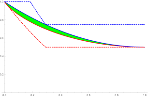
Let us consider one more example. A channel that has recently proven useful in investigating the properties of quantum capacities is the dephrasure channel [50],
| (3.57) |
We can easily get a lower bound on the contraction coefficient by picking the input state in Equation 3.33. An upper bound can either be found from using Lemma 3.6 or Lemma 3.7 (for the latter note that the dephrasure channel can directly be written as a flag channel). Together we get,
| (3.58) |
Finally, a simple observation is that a replacer channel that always outputs a state ,
| (3.59) |
is the noisiest channel and an isometric channel for some isometry is the least noisy channel:
Lemma 3.13.
For any channel , replacer channel and isometric channel , we have
| (3.60) | |||
| (3.61) | |||
| (3.62) |
where the final line implies a similar statement for all other partial orders defined here via Proposition 3.2.
Proof.
Note that
| (3.63) | ||||
| (3.64) | ||||
| (3.65) |
by additivity, faithfulness and data processing of the relative entropy. The proof of the first two lines follows easily from there. The third line is obvious by choosing in the first step and in the second step as the degrading maps. ∎
4 Approximate partial orders and capacities
In this section, we explore approximations of the partial orders introduced in Section 2. These are powerful tools which can be used for instance in approximating capacities of a quantum channel in terms of the ones of another channel when the latter are simpler to compute.
4.1 Approximate partial orders
We recall that the diamond norm distance between two quantum channels is defined as
Previously, Sutter et. al. [78] defined -approximate degradation as follows.
Definition 4.1.
A channel is said to be an -degraded version of if there exists a channel such that .
Now, one can also define approximate versions of other partial orders, as we will do in the following.
Definition 4.2.
A channel is said to be -completely less noisy than (denoted ) if
| (4.1) |
-regularized less noisy than (denoted ) if
| (4.2) |
-less noisy than (denoted ) if
| (4.3) |
-fully quantum less noisy than (denoted ) if
| (4.4) |
One defines similarly the approximate versions of the different more capable orders introduced in Section 2. -anti orders are defined in the same way by exchanging and .
Following the same arguments as in the exact case, see Proposition 3.2, we have immediately that
| (4.5) | ||||||
| (4.6) |
We would of course hope that -approximate degradability implies the above orders. This is indeed the case as we will see in a moment. To relate the two partial orders we will make use of the continuity bounds introduced in [2] and [92]. In what follows, , , denotes the binary entropy.
Lemma 4.3 (Continuity bound, Theorem 1 in [2]).
For quantum states and , if , then
| (4.7) |
Lemma 4.4 (Alicki-Fannes-Winter bound, Lemma 2 in [92]).
For quantum states and , if , then
| (4.8) |
where we recall that the conditional entropy of a state is defined as .
This allows us to directly show the following relation.
Lemma 4.5.
If is an -degraded version of then is -completely less noisy than , with
Therefore,
Proof.
We assume that and start with an input state . Define and . First, observe the following:
where the first inequality follows by data-processing to remove the degrading map. The first equality follows by the definition of the mutual information, the second by adding a zero twice and the fact that and the last inequality by applying Lemma 4.4 twice. The second claim follows from (4.5). ∎
In the same manner, one can go via the fully quantum less noisy order.
Lemma 4.6.
If is an -degraded version of then is -fully quantum less noisy than , with
Therefore,
Proof.
We assume that and start with an input state . Define and . First, observe the following:
where the first inequality follows by data-processing to remove the degrading map, the first equality is by definition of the mutual information, the second by adding a zero once and the fact that , the last inequality by applying Lemma 4.3 and Lemma 4.4. The second claim follows from (4.5). ∎
Clearly, the diamond norm is symmetric under exchanging the arguments. This motivates the following definition.
Definition 4.7.
Two channels and are said to be comparably -completely less noisy if and also , and similarly for comparably - regularized less noisy and comparably - less noisy.
Corollary 4.8.
Assuming , if , then and are comparably -completely less noisy, with .
Proof.
This follows easily by Lemma 4.5 and the symmetry of the diamond norm. ∎
As a special case, of course also the non-complete version is implied. Furthermore, it can be easily seen that -completely less noisy implies -completely more capable. Again, the same holds for the non-complete case. In a similar way, we can directly derive a few other Lemmas.
Lemma 4.9.
If is an -anti-degraded version of , then is -anti-completely less noisy than , with .
Proof.
The proof follows by simply exchanging the roles of and in the proof of Lemma 4.5. ∎
Lemma 4.10.
If is an -conjugate degraded version of , then is -completely less noisy than , with .
Proof.
We again use the same technique as in the proof of Lemma 4.5. However, we need one additional step. Since we only want to show that a less noisy type ordering is implied we can restrict the input state to be classical-quantum. It needs to be shown that going from to does not change the mutual information, where is the conjugation map. We have that,
| (4.9) | ||||
| (4.10) |
Now, since it follows that the mutual information remains unchanged. ∎
4.2 Approximating capacities of a quantum channel
Next, we consider a quantum channel with associated complementary channel 444For detailed definitions, we refer to [88].. We want to investigate properties of the private capacity and the quantum capacity . Let us start with the following.
Theorem 4.11.
Let be a quantum channel.
-
(i)
If is -more capable, then .
-
(ii)
If is -regularized more capable, then .
-
(iii)
If is -fully quantum less noisy, then
-
(iv)
If is -fully quantum less noisy and -regularized more capable, then
Proof.
The proof of the first part is similar to that of [85, Proposition 1]. The second part is simply the same proof for arbitrary and taking the limit, see also [85, Theorem 1]. The third part is similar to the proof of [19, Proposition J.1]. Finally, the last part follows directly from the previous bounds. ∎
To compare the above results to [78, Theorem 3.4], we can easily make the following corollary:
Corollary 4.12.
Let be either -degradable or -conjugate degradable. Then we have
| (4.11) | |||
| (4.12) | |||
| (4.13) | |||
| (4.14) |
with
| (4.15) | ||||
| (4.16) |
Proof.
Follows directly from Theorem 4.11 and Lemma 4.6. ∎
We can furthermore bound the quantum and private capacity of almost anti-less noisy or anti-more capable channels.
Theorem 4.13.
Let be a quantum channel.
-
(i)
be -anti more capable. Then .
-
(ii)
If is -regularized anti more capable, then .
-
(iii)
If be -anti less noisy, then .
-
(iv)
If is -regularized anti less noisy, then .
Proof.
The first two bounds follow immediately by noting that the coherent information can be written as a difference of two mutual informations (see e.g. [88, Theorem 13.6.1]):
| (4.17) |
The proof of the next two bounds follows immediately from the definitions of the private information and the less noisy partial order. ∎
Again, this immediately implies the previously known results about degradable channels (and adding analog ones for conjugate degradable).
Corollary 4.14.
Let be either -anti degradable or -conjugate anti degradable. Then we have
| (4.18) | |||
| (4.19) |
with
| (4.20) | ||||
| (4.21) |
This should be compared to [78, Theorem 3.8].
In a similar fashion we can also reproduce the results in [49].
Lemma 4.15.
If is -less noisy than , we have
| (4.22) |
If is -regularized less noisy than , we have
| (4.23) |
If and are comparably -regularized less noisy and is weakly additive, we have
| (4.24) |
If is -fully quantum more capable than , we have
| (4.25) |
Proof.
The first two statements essentially follow by definition of the involved quantities. The third statement follows by chaining them together and applying the additivity:
| (4.26) |
The final statement again follows trivially from the definitions. ∎
Combining the previous results we easily get the following corollary.
Corollary 4.16.
If and is weakly additive, we have
| (4.27) |
| (4.28) | ||||
| (4.29) |
Proof.
This follows along Equation (4.26) and noting that the final inequality only requires the unregularized -less noisy property. ∎
5 Characterizations of strong data processing
As we discussed in Sec. 2.2, it is possible to show that a channel is less noisy than another channel by considering their respective contraction coefficients. Thus, contraction coefficients can be used to determine if two channels are related in the order. In this section we will now gather characterizations and new properties of contraction coefficients that are of interest beyond the study of partial orders. Indeed, SDPIs are now also becoming a standard tool to understand the computational power of noisy quantum devices [33, 83, 82, 26] and for that application tensorization is also key.
5.1 SDPI via hypercontractivity
Let us prove some characterizations of strong data processing inequalities (SDPI), i.e. the relative entropy contraction coefficient. Obtaining characterizations of strong SDPIs has been the focus of recent activity in quantum information theory. For instance, in [7] the authors show that for a channel :
and
are equivalent. Here we will focus on a hypercontractive approach. In short, hypercontractive inequalities are bounds on various norms of quantum channels . As we will see, these bounds are closely related to entropic inequalities for the channel. But by reducing an entropic inequality to a norm inequality it is often easier to obtain tensorization.
In the classical setting, results connecting hypercontractivity of a Markov kernel and SDPIs go back to Alswede and Gács [1] and have also been the focus of the more recent paper [73, Theorem 6]. In order to state our results, let us define the weighted -quasi-norms for and as:
For these quantities are norms, while for only quasi-norms. They are closely related to the sandwiched Rényi divergences of [63, 91], which can be defined as
for and are known to satisfy a data processing inequality for [3]. Moreover, we have that as , they converge to the usual relative entropy and that these entropies are monotone increasing in the parameter [63]. The connection between these norms and Rényi divergences will allow us to obtain several conditions that imply bounds on the relative entropy contraction coefficients and the less noisy ordering based on the Petz recovery map of the channel. For a quantum channel and a reference state , define with the convention and the Petz recovery map as
We omit the reference state in the definition, as it should always be clear from the context. One can readily check that restricting to the support of it is a quantum channel that satisfies and it is known that if , then [70]. That is, the relative entropy does not contract under if and only if one can reverse the action of the channel on two input states simultaneously with the Petz recovery map.
Our techniques will mostly be based on studying how the norms contract for different values of and reference states under the Petz recovery map. Such statements are intimately related to strong data processing inequalities. Indeed, as shown in [61], the data-processing inequality for the Rényi divergences is equivalent to the statement that for all choices of input state and channels . The basic idea of this section is that if the inequality
| (5.1) |
holds for , then we also obtain a strong data processing inequality for and some Rényi entropy. Note that this statement is stronger than the one with , as the norms are monotone increasing in . Denote by the Hölder conjugates of . One can show by duality of norms that Eq. (5.1) is in fact equivalent to
| (5.2) |
for all states . As we will see in Proposition (5.4), the expression above is equivalent to an SDPI for Rényi entropies.
We start with the following standard Lemma:
Lemma 5.1.
For any two quantum states s.t. we have:
Proof.
Note that
where is the sandwiched Renyi divergence. Define the functions
As and we have:
As , it follows that
which yields the claim after noting that . ∎
The following characterization of a strong DPI then follows:
Proposition 5.2.
For some and a quantum channel , let be the Petz recovery map with respect to . Then the following are equivalent:
-
1.
We have for all
(5.3) -
2.
there exists an s.t. for all we have
(5.4) -
3.
there exists an s.t. for all we have
(5.5)
Proof.
Let us start by showing that (5.4) implies (5.3). Note that by setting , (5.4) gives:
Taking the logarithm and rewriting the Equation above in terms of sandwiched Renyi divergences gives
and Eq. (5.9) follows by taking the limit . Let us show the other direction. It follows from Lemma 5.1 and a Taylor expansion that
from which it follows that
for all small enough. The claim follows from the fact that is suffices to restrict to positive operators when computing norms of completely positive maps [69]. Finally, Eq. (5.5) follows from a duality argument. Indeed, it is easy to show that Eq. (5.4) is equivalent to Eq. (5.2). Taking the logarithm, we obtain the inequality in terms of the Petz recovery map. ∎
Thus, we see that an SDPI is equivalent to a nontrivial inequality for the Petz recovery map for for all slightly larger than . We also immediately obtain a contractive characterization of the less noisy order:
Corollary 5.3.
Let be two quantum channels. Then the following are equivalent:
-
1.
-
2.
For all there and there exists an such that for all we have:
(5.6)
Proof.
It is straightforward to adapt the results above to the completely less noisy ordering by suitably adapting the involved channels and states.
However, it might be difficult to compute the norms analytically, as it is more convenient to work with integer values of . Thus, we will show that any nontrivial inequality gives rise to an SDPI, possibly with an error term.
Proposition 5.4.
Suppose that for some , and two channels , where we assume that is invertible, we have
| (5.7) |
and
| (5.8) |
Then
| (5.9) |
Proof.
Combining Eq. (5.7), Eq. (5.8) and the Stein-Weiss interpolation theorem (see e.g. [61] for a quantum information friendly exposition) yields that:
| (5.10) |
with
for , which can be rewritten as:
| (5.11) |
for all . Solving for and we see that
Taking the logarithm of Eq. (5.11) and rewriting in terms of Rényi entropies we see that
| (5.12) |
A close inspection of the expressions involved in the formula above shows that:
The claim then follows by taking the limit in Eq. (5.12) and noting that and . ∎
For any quantum channel we have by the Russ-Dye theorem that
and, thus, Eq.(5.8) is always satisfied for . That is, if we wish to prove an SDPI for a quantum channel with and additive error term, a inequality suffices.
The case of norms of the Proposition above is particularly interesting, as it leads to entropic inequalities that tensorize:
Corollary 5.5.
Suppose that is invertible as a linear map. Then for some ,
| (5.13) |
implies that for all states
| (5.14) |
Proof.
Define and . Note that Eq. (5.13) is equivalent to
We can further massage this to
| (5.15) |
for all operators . To see this, set . Moreover, we have
Thus, we conclude that for all we have:
Picking and taking the logarithm yields the claim for . The claim for other follows from noting that the condition in Eq. (5.13) tensorizes. Indeed, note that for and we have:
The last equality follows from the fact that the norm just corresponds to the operator norm of the map, which is multiplicative. ∎
Note that the condition in Eq. (5.13) is equivalent to the operator norm of being bounded by . In particular, this means that it can be verified efficiently given the channels and a target state . Thus, we have identified a condition that implies a strong data processing inequality with the feature that it can both be verified efficiently and tensorizes.
This statement can also be used to obtain contraction coefficients that tensorize:
Corollary 5.6.
For some let be the channel and suppose that
| (5.16) |
Then for all states
with .
Proof.
The statement above can be used to bound capacities and entropic quantities of a quantum channel efficiently. For instance, if the channel on a -dimensional space is doubly stochastic, we immediately see that if , then
By noting that , we immediately obtain that the minimum output entropy of is lower bounded by
Inspecting the expression more closely, we see that:
Thus, we see that if and only if the singular values of are contained in a ball of radius around the origin in the complex plane. The largest value of for which this holds is called the spectral gap of .
6 Generalized contraction coefficients and partial orders
In this section we will discuss extensions of the concepts discussed to other divergences, in particular -divergences and -divergences. Note that both partial orders and contraction coefficients can be naturally defined in terms of any divergence by simply replacing the relative entropy by the desired divergence.
Interestingly, classically contraction coefficients (and partial orders respectively) based on many different divergences have been shown actually to be the same, see e.g. [55]. In the quantum case this remains a mostly open problem with some of what is known being summarized in the following section.
6.1 f-divergences
Here, we extend the discussions of the previous sections to the setting of arbitrary -divergences [67, Chapter 7]. The two most commonly used ones are the standard -divergence: given with full-rank:
| (6.1) |
where is the so-called relative modular operator between states and and can be interpreted as a non-commutative generalization of the Radon-Nikodym derivative between two probability mass functions. Similarly, the maximal -divergence is defined as
| (6.2) |
Note that, often, only those functions that obey are considered valid for f-divergences as it ensures that . However, this excludes e.g. Rényi divergences.
Of course, we can define contraction coefficients and as for other divergences. Next, we want to consider mutual information like quantities based on f-divergences. Consider the following definitions,
| (6.3) | ||||
| (6.4) |
In what follows, we denote resp. for either or , resp. or . Note, that just like for the relative entropy, the following holds. Consider a classical quantum state and its marginal , we have
| (6.5) |
As a direct consequence, for a quantum channel , we have
| (6.6) |
resulting in
| (6.7) |
Before proving the equivalence of Proposition 6.2, we recall this very simple technical lemma:
Lemma 6.1.
Let be a self-adjoint operator over a finite dimensional Hilbert space, and let be a function on that is differentiable at . Then
Proof.
Simply write the eigenvalue decomposition of , so that
∎
The next Proposition is a direct generalization of Theorem 5.2 in [74]
Proposition 6.2.
Let be differentiable, and let and , and . The following are equivalent:
-
(i)
For all states with marginal , where is an arbitrary classical system,
-
(ii)
For any state with ,
(6.8)
Therefore, if and only if Equation 6.8 holds for .
Proof.
We first prove (ii)(i): for any and conditional states , we have
where is defined to be the marginal of . Then the result follows directly from (ii). Next, we prove that (i)(ii): without loss of generality we assume that is full-rank. Then, for any , and , where is small enough to ensure that , we let be the binary random variable of distribution , , and conditional states , . Clearly we have that .
Then, let
Since when , we have that . Moreover, (i) implies that for any . Since from , we have that . The result follows after computing the latter derivative:
We will be done as soon as we can show that the derivative above is equal to . By linearity of the channels and , it is enough to show that
We first focus the case of the maximal -divergences: we have
| (6.9) | ||||
| (6.10) | ||||
| (6.11) |
where the second identity comes from Lemma 6.1. It is then straightforward to evaluate the derivative above and verify that
which gives what we needed to prove. The case of the standard -divergence can be treated similarly:
where in we used once again Lemma 6.1 in (1).
∎
Remark 6.3.
The previous result can be easily extended to the case of optimized quantum divergences as defined in [89].
Remark 6.4.
Note that we only require to be differentiable. Thus, Proposition 6.2 holds for a larger class of functionals than divergences.
As a result we can express the contraction coefficient based on -divergences in terms of the corresponding -mutual information
| (6.12) |
as well as define partial orders based on -mutual informations that can be equivalently formulated in terms of -divergences. We will denote these by .
Let us end this section by discussing our favorite example: the erasure channel. One can easily find the following.
Lemma 6.5.
For any function with , we have
| (6.13) | ||||
| (6.14) |
which immediately implies that for all functions and with the above property, we have
| (6.15) |
Proof.
By direct calculation. ∎
This implies that we can easily extend our previous Proposition 2.5.
Proposition 6.6.
Let , and any function with . Then the following are equivalent:
-
(i)
.
-
(ii)
.
Proof.
Analog to that of Proposition 2.5. ∎
And the same holds for the maximal -divergence.
6.2 Spectral approaches to quantum less-noisy pre-orders
In Theorem 1 of [55], it was shown in the classical setting that the less noisy pre-order is equivalent to the following condition: for any probability mass functions
where the divergence is defined as follows:
| (6.16) |
This characterization is powerful as it allows for a spectral analysis of the less noisy pre-order [55]. The proof of this fact relies on two observations: to prove that less noisiness implies (6.16), it uses the characterization of less noisy seen in Section 2.2, namely that is equivalent to
| (6.17) |
for any two probability mass functions and , together with the well-known fact that the divergence locally approximates the relative entropy:
| (6.18) |
On the other hand, the relative entropy can be rewritten in terms of the following integral [55] (see also [58, 64, 65] for slightly different related expressions):
| (6.19) |
The characterization of less noisiness in terms Equation 6.16 follows from the joint use of Equations 6.18 and 6.19. This result implies as a special case the following result [14] (see also refinements, e.g. Theorem 3.6 of [74], and [74, 1] for the link to the contraction coefficient for the maximal correlation):
| (6.20) |
The quantity is known classically to locally approximate any divergence [10, 13]. This is no longer the case in the non-commutative world, where a complete characterization of quantities, also known as Fisher information metrics, was found [52, 79]. First of all, we define the following set of functions:
Next, for , and , define the quantum -divergence
when , and infinity otherwise. In the previous case, the inversion is defined as
Here, we also restrict ourselves to a subclass of -divergences: consider the class of continuous operator convex functions from to that satisfy . These functions can all be expressed in terms of the following integral representation:
| (6.21) |
where and the integral of the positive measure on is bounded. Then, for any , there exists such that [52, 79]:
| (6.22) |
The function is related to by
| (6.23) |
Hence, like its classical restriction, the quantum divergence can be understood as a local approximation of the quantum relative entropy. However, Equation 6.19 is not known to hold in general in the quantum case. Rather, the following integral representation of the quantum relative entropy is known and has been recently used to get tightenings of the data processing inequality in [12] as a special case of the integral representation (6.21):
| (6.24) |
It can be easily shown that the integrands in Equation 6.24 and Equation 6.19 coincide when and commute and can be identified with and . However, the integrand (6.24) cannot be identified in general with an adequately normalized divergence. In particular, Equation 6.20 is not known to hold in general in the quantum setting, despite some recent progress in that direction [51, 37]. We also refer to the more recent paper [11] where the strong data processing for the divergence was shown to tensorize in the case where the state is taken to be a tensor product.
For the reasons mentioned above, it seems unlikely that the equivalence between less noisy and the ordering of is true in the quantum setting. However, the following result is a direct consequence of the above discussion:
Proposition 6.7.
For any two quantum channels and , , where:
-
For any two quantum states and any :
-
For all and any two states :
-
For any and any two quantum states ,
Moreover, if (ii) holds only for a given , then (iii) holds for satisfying (6.23). Finally, obvious extensions of the above chain of implications hold true in the case of regularized and complete less noisy pre-orders, as well as for the related contraction coefficients.
Finally, we will once more mention the erasure channel as an illustrating example.
Lemma 6.8.
Let be the quantum erasure channel of parameter , and be some quantum states. Then for any we have that
| (6.25) |
Therefore,
This means that at least for the erasure channel the contraction coefficients for relative entropy, f-divergences and divergence are the same.
7 Functional inequalities
Another standard way of obtaining strong data processing is through functional inequalities [73], which we will describe in a bit more detail below. This approach is particularly effective whenever we have a semigroup converging to a unique full rank state . Such semigroups are called primitive. In [55] the authors relate such functional inequalities to the less noisy ordering in the classical setting, especially when comparing to symmetric channels. Here we will recover their results in the quantum setting, especially Proposition 12, while also revisiting the connections between functional and entropic inequalities.
We will start by defining logarithmic Sobolev inequalities and showing their consequences. Let be a primitive channel whose unique invariant state is , and denote by the corresponding completely, positive unital dual map. Corresponding to the map , we construct a quantum Markov semigroup (QMS) of completely positive unital maps for all . In other words, the resulting semigroup has as its generator. The semigroup is by construction also primitive, and is its unique invariant state. We can then define a scalar product
which induces the norm. Next we define the Dirichlet form corresponding to as follows: for all ,
Next, we define the -entropy as follows: for any ,
where here the relative entropy has been extended to non-normalized positive operators whenever . The QMS satisfies the logarithmic Sobolev inequality (LSI) if there exists such that for every
| (7.1) |
The largest such that Equation 7.1 holds
is called the logarithmic Sobolev constant of . Likewise, the logarithmic Sobolev inequality for the discrete-time Markov chain with constant states that for every ,
where is sometimes referred to as the discrete Dirichlet form. Logarithmic Sobolev inequalities are particularly useful for reversible semigroups, i.e. semigroups such that their Petz recovery map with respect to the invariant state is the semigroup itself. In this case, it is known that a LSI implies the following hypercontractive inequality:
| (7.2) |
By the results of Proposition 5.4, we know that this can be used to obtain strong data processing inequalities involving Rényi divergences. Indeed, we immediately obtain:
Nevertheless, the inequality above is a bit unsatisfactory, as it does not give complete contraction even as . But this can be easily remedied by resorting to reversibility. As the semigroup is reversible, Eq. (7.2) also implies
| (7.3) |
by duality. By Proposition 5.4, we conclude that:
Exploiting the fact that we then get an exponential decay of the relative entropy from the logarithmic Sobolev inequality. Although this result is by no means new [31, 68, 46], we believe that the approach presented here showcases transparently how a LSI implies several different entropic inequalities. Computing the LSI constant is, in general, an arduous task. For the depolarizing semigroup in dimension , it is known that:
| (7.4) |
It is possible to obtain estimates of LSI through 7.4 for any doubly stochastic channel through so-called comparison techniques. The same is true for generalized depolarizing channels.
Indeed, an easy way of estimating the LSI constant of a semigroup assuming that we know the LSI constant of another QMS is via the comparison of their Dirichlet forms: assume that and have the same unique invariant state , then:
In the next theorem, we show that the information-theoretic notion of less noisy domination is a sufficient condition for the comparison of Dirichlet forms. First, we recall the following Lemma from [55]:
Lemma 7.1.
Given a positive semi-definite real matrix and a normal real matrix ,
From this we get:
Theorem 7.2.
Let be two primitive quantum channels, with a common unique full-rank invariant state . Then the following are true:
-
(i)
If , then:
or equivalently
for all states .
-
(ii)
Assume that is positive semi-definite on and that . If , then for all
-
(iii)
Assume that , with the generalized depolarizing channel with depolarizing probability to a state , and for some channel with as its stationary state. Then:
Proof.
(i) We use the implication of Proposition 6.7 in order to get that implies that for any two states
This implies, taking and that
Note that the adjoint of with respect to the weighted scalar product is . Thus, we can rewrite this last condition as follows:
(ii) The previously proved result implies in particular that the maps and seen as matrices acting on the real vector space of self-adjoint operators provided with the -KMS inner product ,
From Lemma 7.1, we find that
(iii) Note that for the depolarizing channel. Thus, the assumptions of (ii) are fulfilled. The claim then follows by a simple manipulation. ∎
Note that is nothing but the variance of the observable with respect to the state . Thus, we conclude that from a less-noisy comparison between channels with the same invariant state we immediately get a comparison of Dirichlet forms and a bound on logarithmic Sobolev constants if one of them is known. Unfortunately, such techniques do not yield sharp inequalities for the SDPI constant for channels. This is because it is known that for generalized depolarizing channels, we have that the optimal SDPI constant [62] is given by:
where
with the smallest eigenvalue of and
where is the binary relative entropy. Moreover, for qubit depolarizing channels we have and we know that satisfies a SDPI with constant [4]. This is to be contrasted with the LS estimate, which decays with the local dimension.
8 Special classes of channels
8.1 Weyl-covariant channels
In this section, we provide new comparison bounds for Weyl-covariant channels [87, 23, 42, 43] (see also [86]). We consider the finite group with the following projective representation on :
Next, define the discrete Fourier transform to be the following unitary matrix on
A map on is a Weyl-covariant map if
for every and . In particular, any additive noise channel of the form
| (8.1) |
where is a probability mass function, is Weyl-covariant, by the irreducibility of the representation . Moreover, one can show that any Weyl-covariant channel has this form (see Corollary 4.15 in [86]). The next Lemma is an extension of Lemma 1 in [55]:
Lemma 8.1.
Any two Weyl-covariant noise channels and satisfy if and only if there exists a probability distribution function on such that .
Proof.
We simply need to prove the forward implication. By definition, there exists a channel such that . Now, for any , since where ,
| (8.2) | ||||
| (8.3) | ||||
| (8.4) |
On the other hand, . Assume first that for some . Then from the degradability condition, and we can choose without loss of generality . Now, assume that . Then we have . Therefore, we found that there exists a function such that for all , . We conclude by an appeal to Theorem 4.14 in [86].
∎
In Section 2.1, we introduced the notion of a less noisy domination region. Restricting ourselves to comparisons with additive noise channels, we can also define the so-called additive less noisy domination region of a channel acting on system as
and its additive degradation region
where both are subsets of the set of Weyl-covariant channels of the form of (8.1).
Proposition 8.2.
Let be a Weyl-covariant quantum channel corresponding to the probability distribution function . Then, and are non-empty, closed, convex, and invariant under the conjugate action of : for all ,
where . Moreover, .
Proof.
Non-emptiness, closure and convexity follow in the same way as in Proposition 2.2 in addition with the fact that the set of additive noise channels is closed and convex. Invariance under the conjugate action of the Weyl operators is also apparent. The identity in (2) follows from Lemma 8.1. ∎
In the case when is the distribution
the map reduces to
with . This is the depolarizing channel of noise parameter . We recall that this map is completely positive if and only if , i.e. if and only if [45, 48]. Moreover, the family forms a semigroup: . From this property, one can easily derive that for ,
| (8.5) |
In the next result, we prove that a depolarizing channel can never be less noisy than an erasure channel, hence extending Proposition 7 of [55]:
Proposition 8.3.
For , given an erasure channel with erasure probability , there does not exist such that the corresponding depolarizing channel satisfies .
Proof.
For an erasure channel with , we always have . On the other hand, for any , we have for all . Hence for any by the characterization in Proposition 2.3. ∎
As we saw in Proposition 3.2, degradability is at least as strong as any notion of less noisy ordering. This raises the question of whether one can find pair of channels such that without . In the next result, we make one step towards this direction by proving a separation between the (non-complete) less noisy ordering and degradability between two quantum channels. This result extends Proposition 11 of [55]:
Proposition 8.4.
Given a Weyl-covariant channel over , , and
If is a convex mixture of the channels and , , then
Remark 8.5.
Choosing to be the depolarizing channel , we already saw in (8.5) that , and hence , whenever . Therefore, since , Proposition 8.4 provides us with a class of channels that belong to . However the problem of finding two channels such that but still remains open, even when the channels and are taken to be classical.
Proof.
Thanks to Proposition 8.2, it is enough to prove that . Then, by the characterization in Proposition 2.3, we simply need to show that for any two states ,
Denoting by and the eigenvalue decompositions of the states, we can easily show that the above relative entropies are linear functions of the square overlaps between the eigenvectors of and those of . For instance, denoting by , we have
| (8.6) |
where and . Hence,
Similarly, we denote by and define and as the corresponding convex mixtures of the eigenvalues of , resp. and the ones of the completely mixed state. Denote by the matrix whose entropies are given by . Since both and form orthonormal bases, is doubly stochastic. Then, by Birkhoff’s theorem, can be written as a convex combination of permutation matrices. Therefore, we can conclude that if an inequality of the form
holds for all permutation matrices , then it holds for all doubly stochastic matrices , and therefore (8.6) holds for all states . However, restricting to the case of permutation matrices means that we can, without loss of generality, assume that the states and commute. In other words, we reduced the proof to that of classical depolarizing channels over classical probability mass functions, for which we can directly invoke Proposition 11 in [55]. ∎
8.2 Gaussian channels
In this section, we consider the setting of Gaussian quantum channels [44]: an -mode quantum system is modeled by the Hilbert space of complex-valued, square-integrable functions on . On this space, we define the so-called creation and annihilation operators, , by means of their commutation relations
where for each , and act nontrivially on the -th copy of the system. The number operator is defined as
and corresponds to the energy of the system. In the case , it is known to have the following spectral decomposition onto the Fock basis :
Next, we denote by the coherent state of parameter . These are the eigenvectors of the one-mode annihilation operator, . In what follows, for a vector , the tensor product of coherent states will be denoted by . The Weyl displacement operators , , are unitary operators that rotate the -mode vacuum state to the coherent state . In terms of the creation and annihilation operators, they are defined as
| (8.7) |
Next, an -mode quantum Gaussian state is proportional to the exponential of a quadratic polynomial in the creation and annihilation operators. Among these states, thermal Gaussian states play an important role. They are defined by -fold products of the following geometric probability distribution for the energy:
The average energy of is equal to , whereas its entropy is equal to
| (8.8) |
Quantum Gaussian channels are those quantum channels that preserve the set of quantum Gaussian states. The most important classes of such channels are the beam-splitter, the squeezing, quantum Gaussian attenuators and quantum Gaussian amplifiers. The first two are unitary quantum analogs of the operation of linearly mixing random variables: a two-mode beam-splitter of transmissivity is defined by the following action on the ladder operators:
This is a simple example of a passive Gaussian channel in the sense that it preserve the total energy: . On the other hand, the two-mode squeezing of parameter increases the energy of the input. It is defined similarly to the beam-splitter as follows:
In both cases, it is standard to interpret the first factor of the tensor product as the system and the second factor as the environment. Next, for , we denote by the reduced state on the system of either the beam-splitter () or the squeezer (). The quantum Gaussian attenuator , of parameters and , corresponds to the channel . Similarly, the quantum Gaussian amplifier of parameters and , corresponds to the channel .
Another important Gaussian channel considered in the literature is the Gaussian additive noise channel. It is generated by a convex combination of displacement operators with a Gaussian probability measure:
| (8.9) |
In fact, the Gaussian additive noise channel can be seen as a large particle number limit of the attenuator channel (see [34]).
All the channels mentioned above are typical examples of a gauge-covariant Gaussian channel [44]: A channel is called gauge-covariant if for all input state ,
where is the gauge transformation corresponding to the -mode harmonic oscillator. In fact, every phase-covariant quantum Gaussian channel can be expressed as a quantum-limited amplifier composed with a quantum-limited attenuator.
The following conjecture, stated in [35], was recently proved in the restricted one-mode case [29, 28] as well as for the range of parameters for which the channels become entanglement-breaking [24]; that is
-
(i)
For any quantum Gaussian attenuator with ;
-
(ii)
For any quantum Gaussian amplifier with ;
-
(iii)
For any quantum Gaussian additive noise channel with .
Conjecture 8.7 (Constrained minimum output entropy conjecture for phase-covariant quantum channels).
For any and any with finite entropy, let be the one-mode thermal Gaussian state with entropy . Then, for any , , :
| (8.10) | |||
| (8.11) | |||
| (8.12) |
In the next result, we provide an exact expression for contraction coefficients of any of these Gaussian channels and their tensor products under the condition that 8.7 holds. More precisely, let , , be one-mode Gaussian states, be a one-mode Gaussian quantum channel, and define the contraction coefficients for the relative entropy as
| (8.13) |
Here, we define the relative entropy as Lindblad in [54, 53]: given any two positive, trace-class operators , if , resp. , is a complete orthonormal set of eigenvectors of with corresponding eigenvalues , resp. with eigenvalues ,
where the sum is taken to be if the series diverges. Furthermore, we define the energy-constrained relative entropy contraction coefficient as follows: for
Theorem 8.8.
Assume that 8.7 holds true. Then for any family of energies, any , , , and :
| (8.14) | |||
Before proving Theorem 8.8, we state and prove a couple of technical lemmas. The first one allows us to restrict the optimization (8.13) to finite-rank input states (see Lemma 21 in [56] for a classical analogue):
Lemma 8.9 (Finite-rank state characterization of ).
Let be the set of finite-rank -mode quantum states supported on . Then for any -mode bosonic channel , and any thermal Gaussian states :
| (8.15) |
Remark 8.10.
Remark that the optimization does not need to assume that : this is automatically true since is faithful, and hence cannot be equal to any finite-rank state.
Proof.
Consider a quantum state such that , and define a sequence of finite-dimensional orthogonal projections on which commute with and such that strongly as (i.e. for all ). Then, for ,
where the identity follows from the fact that by assumption. Now by strong convergence of the sequence , as . Moreover, by Lemma 4 in [54], we have that as . Hence,
| (8.16) |
Moreover, by lower semi-continuity of the quantum relative entropy, we also have that
| (8.17) |
Combining Equation 8.16 and Equation 8.17, we have that
| (8.18) |
The rest of the proof relies on a diagonalization argument that was already used in Lemma 21 in [56]: suppose that is a sequence of quantum states that satisfies for all and achieves the supremum in (8.13):
Then, by (8.18), we can construct a sequence where each is chosen such that for every :
Letting , we end up with
Since the supremum in (8.13) is over a smaller set than in (8.15), the above inequality is actually an equality, and the result follows. ∎
The next technical lemma will serve as a replacement of Bernoulli’s inequality in [56]:
Lemma 8.11.
For any three numbers ,
| (8.19) |
where . Similarly, for any and , we have
| (8.20) |
Proof.
The proof of (8.19) amounts to proving that the function
is monotone decreasing. Now, wince is differentiable, we have
Therefore, after dividing by , we reduced the proof to that of showing that the function is monotone decreasing for all . After differentiation, we further simplify the proof to that of showing that the function
| (8.21) |
is increasing. This last assertion can be showed to hold after differentiating the function defined in (8.21). To obtain (8.20), we simply operate the following replacements in (8.19): , and . Then we are reduced to having to prove that
Using once again the fundamental theorem of calculus and an obvious rescaling, we reduce the problem to that of proving that for all the function
is increasing. By differentiating this function, it is enough to show that the function
on is decreasing. One last differentiation reduces the problem to the basic inequality on . ∎
We are now ready to prove our main result.
Proof of Theorem 8.8.
Step 1: Upper bounding : by Lemma 8.9, we can restrict the optimization to that over finite-rank input states supported on , so that . Such states also have finite von Neumann entropy. Moreover, the energy at the output of any Gaussian quantum channel is also finite [76]. Then given any sequence of thermal Gaussian states, and denoting by the difference in energy between and ,
| (8.22) |
Let us now consider the attenuator channel . Since , we have
| (8.23) |
Hence, for to be upper bounded by the right-hand side of (8.14), it suffices to prove that for any :
By the constrained minimum entropy conjecture (8.10), we can further simplify the problem to that of proving, for any ,
| (8.24) |
The result directly follows from (8.20) for and . The case of the amplifier follow the exact same proof, since .
Now, we turn our attention to the additive noise channel : here, since , (8.23) has to be replaced by
| (8.25) |
Therefore, as previously, by conjecture (8.12) it is enough to prove that for any , denoting by ,
Then, invoking (8.19) for and allows us to conclude.
Step 2: : this is obvious by definition of the contraction coefficients.
Step 3: Lower bounding for all : let us start with the additive noise channel : choosing to be a tensor product state, we can reduce to the case without loss of generality. Moreover, we choose to be the thermal Gaussian state . Then, we have for any displaced thermal state , ,
The lower bound follows after taking , and taking the limit . Since for all , the result follows. The cases of the amplifier and of the attenuator follow the exact same computations. The other two cases follows the exact same argument. ∎
Remark 8.12.
Remark 8.13.
In the classical setting, it is well-known that the contraction coefficient for the classical additive white Gaussian noise channel, even when restricting to inputs of finite energy. In order to get nontrivial contraction, the following non-linear strong data processing inequality was proposed in [71, 21]: for the channel
where the supremum is over all joint distributions with constrained input energy over system . In [21], it was shown that such curves are always strictly less than for all . A similar analysis in the quantum setting will be the subject of future work.
9 Conclusions
In this work, we discussed the relationship between the concept of contraction coefficients and the less noisy partial order. The equivalence between their respective relative entropy and mutual information formulations allowed us a new point of view on their properties and bringing our knowledge in the quantum setting closer to what is currently available in the classical case. Given the central position data processing takes in the field of quantum information theory, we expect our results to lay the ground for further results and applications to plenty information processing tasks. Indeed, the techniques developed here already found applications in obtaining state-of-the-art bounds on the performance of noisy quantum devices [26, 82], novel capacity bounds [38] and the study of quantum differential privacy [40].
Nevertheless, many open questions remain. Most crucially, it is not yet clear whether the relations between the different partial orders are actually strict. For example, we know that
but it is not known whether the opposite directions might also hold, namely
Moreover, the fully quantum less noisy order and the regularized less noisy order sit somewhat parallel in the hierarchy of orders, compare Figure 1. In the exact case, both have been used to e.g. to give a condition for which the quantum capacity becomes single-letter. It would have interesting applications to find a direct relationship between the two orders, i.e. one or both of the following:
Finally, for SDPI constants and contraction coefficients, natural open problems include a better understanding of their tensorization properties and the possible equivalence of constants based on different divergences.
Acknowledgments
CH and DSF acknowledge financial support from the VILLUM FONDEN via the QMATH Centre of Excellence (Grant no. 10059) and the QuantERA ERA-NET Cofund in Quantum Technologies implemented within the European Union’s Horizon 2020 Programme (QuantAlgo project) via the Innovation Fund Denmark. DSF acknowledges financial support from the European Research Council (grant agreement no. 81876). CR is partially supported by a Junior Researcher START Fellowship from the MCQST. CR acknowledges funding by the Deutsche Forschungsgemeinschaft (DFG, German Research Foundation) under Germanys Excellence Strategy EXC-2111 390814868.
References
- [1] Rudolf Ahlswede and Peter Gács. Spreading of sets in product spaces and hypercontraction of the markov operator. The annals of probability, pages 925–939, 1976. doi:10.1214/aop/1176995937.
- [2] Koenraad M R Audenaert. A sharp continuity estimate for the von Neumann entropy. Journal of Physics A: Mathematical and Theoretical, 40(28):8127–8136, June 2007. doi:10.1088/1751-8113/40/28/s18.
- [3] Salman Beigi. Sandwiched Rényi divergence satisfies data processing inequality. Journal of Mathematical Physics, 54(12):122202, jun 2013. URL: http://arxiv.org/abs/1306.5920, arXiv:1306.5920, doi:10.1063/1.4838855.
- [4] Salman Beigi, Nilanjana Datta, and Cambyse Rouzé. Quantum reverse hypercontractivity: Its tensorization and application to strong converses. Communications in Mathematical Physics, 376(2):753–794, 2020. doi:10.1007/s00220-020-03750-z.
- [5] Salman Beigi and Amin Gohari. On dimension bounds for auxiliary quantum systems. IEEE transactions on information theory, 60(1):368–387, 2013. doi:10.1109/TIT.2013.2286079.
- [6] P Bergmans. Random coding theorem for broadcast channels with degraded components. IEEE Transactions on Information Theory, 19(2):197–207, 1973. doi:10.1109/TIT.1973.1054980.
- [7] Mario Berta, David Sutter, and Michael Walter. Quantum Brascamp-Lieb Dualities, 2019. arXiv:1909.02383v2. URL: https://arxiv.org/abs/1909.02383, arXiv:1909.02383, doi:10.48550/ARXIV.1909.02383.
- [8] Francesco Buscemi. Degradable channels, less noisy channels, and quantum statistical morphisms: An equivalence relation. Problems of Information Transmission, 52(3):201–213, 2016. doi:10.1134/s0032946016030017.
- [9] Francesco Buscemi. Comparison of noisy channels and reverse data-processing theorems. In 2017 IEEE Information Theory Workshop (ITW), pages 489–493. IEEE, 2017. doi:10.1109/itw.2017.8278038.
- [10] LL Campbel. An extended Cencov characterization of the information metric. In Proc. AMS, volume 98, pages 135–141, 1996.
- [11] Yu Cao and Jianfeng Lu. Tensorization of the strong data processing inequality for quantum chi-square divergences. Quantum, 3:199, 2019. doi:10.22331/q-2019-10-28-199.
- [12] Eric A Carlen and Anna Vershynina. Recovery map stability for the data processing inequality. Journal of Physics A: Mathematical and Theoretical, 53(3):035204, January 2020. doi:10.1088/1751-8121/ab5ab7.
- [13] Nikolai Nikolaevich Cencov. Statistical decision rules and optimal inference. Number 53. American Mathematical Soc., 2000.
- [14] Man-Duen Choi, Mary Beth Ruskai, and Eugene Seneta. Equivalence of certain entropy contraction coefficients. Linear algebra and its applications, 208:29–36, 1994. doi:10.1016/0024-3795(94)90428-6.
- [15] Matthias Christandl, Christoph Hirche, and Andreas Winter. in preparation. 2021.
- [16] Joel Cohen, Johannes HB Kempermann, and Gheorghe Zbaganu. Comparisons of stochastic matrices with applications in information theory, statistics, economics and population. Springer Science & Business Media, 1998.
- [17] Joel E Cohen, Yoh Iwasa, Gh Rautu, Mary Beth Ruskai, Eugene Seneta, and Gh Zbaganu. Relative entropy under mappings by stochastic matrices. Linear algebra and its applications, 179:211–235, 1993. doi:10.1016/0024-3795(93)90331-h.
- [18] Thomas Cover. Broadcast channels. IEEE Transactions on Information Theory, 18(1):2–14, 1972. doi:10.1109/TIT.1972.1054727.
- [19] Andrew Cross, Ke Li, and Graeme Smith. Uniform additivity in classical and quantum information. Physical review letters, 118(4):040501, 2017. doi:10.1103/physrevlett.118.040501.
- [20] Imre Csiszár and Janos Korner. Broadcast channels with confidential messages. IEEE transactions on information theory, 24(3):339–348, 1978. doi:10.1109/TIT.1978.1055892.
- [21] F. d. P. Calmon, Y. Polyanskiy, and Y. Wu. Strong data processing inequalities for input constrained additive noise channels. IEEE Transactions on Information Theory, 64(3):1879–1892, 2018. doi:10.1109/tit.2017.2782359.
- [22] Nilanjana Datta, Christoph Hirche, and Andreas Winter. Convexity and operational interpretation of the quantum information bottleneck function. In 2019 IEEE International Symposium on Information Theory (ISIT), pages 1157–1161. IEEE, 2019. doi:10.1109/isit.2019.8849518.
- [23] E Brian Davies. On the repeated measurement of continuous observables in quantum mechanics. Journal of Functional Analysis, 6(2):318–346, 1970. doi:10.1016/0022-1236(70)90064-9.
- [24] G. De Palma. New lower bounds to the output entropy of multi-mode quantum gaussian channels. IEEE Transactions on Information Theory, 65(9):5959–5968, 2019. doi:10.1109/tit.2019.2914434.
- [25] Giacomo De Palma and Stefan Huber. The conditional entropy power inequality for quantum additive noise channels. Journal of Mathematical Physics, 59(12):122201, 2018. doi:10.1063/1.5027495.
- [26] Giacomo De Palma, Milad Marvian, Cambyse Rouzé, and Daniel Stilck França. Limitations of variational quantum algorithms: a quantum optimal transport approach, 2022. arXiv.2204.03455. doi:10.48550/ARXIV.2204.03455.
- [27] Giacomo De Palma and Dario Trevisan. The conditional entropy power inequality for bosonic quantum systems. Communications in Mathematical Physics, 360(2):639–662, 2018. doi:10.1007/s00220-017-3082-8.
- [28] Giacomo De Palma, Dario Trevisan, and Vittorio Giovannetti. Gaussian states minimize the output entropy of the one-mode quantum attenuator. IEEE Transactions on Information Theory, 63(1):728–737, 2016. doi:10.1109/tit.2016.2621748.
- [29] Giacomo De Palma, Dario Trevisan, and Vittorio Giovannetti. Gaussian states minimize the output entropy of one-mode quantum gaussian channels. Physical review letters, 118(16):160503, 2017. doi:10.1103/PhysRevLett.118.160503.
- [30] Pierre Del Moral, Michel Ledoux, and Laurent Miclo. On contraction properties of Markov kernels. Probability theory and related fields, 126(3):395–420, 2003. doi:10.1007/s00440-003-0270-6.
- [31] P. Diaconis and L. Saloff-Coste. Logarithmic Sobolev inequalities for finite Markov chains. Ann. Appl. Probab., 6(3):695–750, 08 1996. URL: http://dx.doi.org/10.1214/aoap/1034968224, doi:10.1214/aoap/1034968224.
- [32] Marco Fanizza, Farzad Kianvash, and Vittorio Giovannetti. Quantum flags and new bounds on the quantum capacity of the depolarizing channel. Physical Review Letters, 125(2), July 2020. doi:10.1103/physrevlett.125.020503.
- [33] Daniel Stilck França and Raul García-Patrón. Limitations of optimization algorithms on noisy quantum devices. Nature Physics, 17(11):1221–1227, oct 2021. doi:10.1038/s41567-021-01356-3.
- [34] Vittorio Giovannetti, Saikat Guha, Seth Lloyd, Lorenzo Maccone, and Jeffrey H Shapiro. Minimum output entropy of bosonic channels: a conjecture. Physical Review A, 70(3):032315, 2004. doi:10.1103/physreva.70.032315.
- [35] Saikat Guha, Jeffrey H Shapiro, and Baris I Erkmen. Classical capacity of bosonic broadcast communication and a minimum output entropy conjecture. Physical Review A, 76(3):032303, 2007. doi:10.1103/physreva.76.032303.
- [36] Fumio Hiai and Dénes Petz. The proper formula for relative entropy and its asymptotics in quantum probability. Comm. Math. Phys., 143(1):99–114, 1991. URL: http://projecteuclid.org/euclid.cmp/1104248844, doi:10.1007/BF02100287.
- [37] Fumio Hiai and Mary Beth Ruskai. Contraction coefficients for noisy quantum channels. Journal of Mathematical Physics, 57(1):015211, 2016. doi:10.1063/1.4936215.
- [38] Christoph Hirche and Felix Leditzky. Bounding quantum capacities via partial orders and complementarity. February 2022. arXiv:2202.11688, doi:10.1109/ISIT50566.2022.9834698.
- [39] Christoph Hirche and David Reeb. Bounds on information combining with quantum side information. IEEE Transactions on Information Theory, 64(7):4739–4757, 2018. doi:10.1109/tit.2018.2842180.
- [40] Christoph Hirche, Cambyse Rouzé, and Daniel Stilck França. Quantum differential privacy: An information theory perspective. February 2022. arXiv:2202.10717.
- [41] Christoph Hirche and Andreas Winter. An alphabet-size bound for the information bottleneck function. In 2020 IEEE International Symposium on Information Theory (ISIT), pages 2383–2388. IEEE, 2020. doi:10.1109/isit44484.2020.9174416.
- [42] Alexander S Holevo. A note on covariant dynamical semigroups. Reports on mathematical physics, 32(2):211–216, 1993. doi:10.1016/0034-4877(93)90014-6.
- [43] Alexander S Holevo. Covariant quantum markovian evolutions. Journal of Mathematical Physics, 37(4):1812–1832, 1996. doi:10.1063/1.531481.
- [44] Alexander S Holevo. Quantum systems, channels, information: a mathematical introduction, volume 16. Walter de Gruyter, 2012. doi:10.1515/9783110273403.
- [45] Michał Horodecki and Paweł Horodecki. Reduction criterion of separability and limits for a class of distillation protocols. Physical Review A, 59(6):4206, 1999. doi:10.1103/PhysRevA.59.4206.
- [46] Michael J. Kastoryano and Kristan Temme. Quantum logarithmic Sobolev inequalities and rapid mixing. Journal of Mathematical Physics, 54(5), 2013. arXiv:1207.3261, doi:10.1063/1.4804995.
- [47] J Korner and K Marton. Comparison of two noisy channels. Topics in information theory, pages 411–423, 1977.
- [48] Ludovico Lami and Marcus Huber. Bipartite depolarizing maps. Journal of Mathematical Physics, 57(9):092201, 2016. doi:10.1063/1.4962339.
- [49] Felix Leditzky, Eneet Kaur, Nilanjana Datta, and Mark M Wilde. Approaches for approximate additivity of the holevo information of quantum channels. Physical Review A, 97(1):012332, 2018. doi:10.1103/PhysRevA.97.012332.
- [50] Felix Leditzky, Debbie Leung, and Graeme Smith. Dephrasure channel and superadditivity of coherent information. Physical review letters, 121(16):160501, 2018. doi:10.1103/PhysRevLett.121.160501.
- [51] Andrew Lesniewski and Mary Beth Ruskai. Monotone riemannian metrics and relative entropy on noncommutative probability spaces. Journal of Mathematical Physics, 40(11):5702–5724, November 1999. doi:10.1063/1.533053.
- [52] Andrew Lesniewski and Mary Beth Ruskai. Monotone Riemannian metrics and relative entropy on noncommutative probability spaces. Journal of Mathematical Physics, 40(11):5702–5724, 1999. doi:10.1063/1.533053.
- [53] Göran Lindblad. Entropy, information and quantum measurements. Communications in Mathematical Physics, 33(4):305–322, 1973. doi:10.1007/BF01646743.
- [54] Göran Lindblad. Expectations and entropy inequalities for finite quantum systems. Communications in Mathematical Physics, 39(2):111–119, 1974. doi:10.1007/BF01608390.
- [55] Anuran Makur and Yury Polyanskiy. Comparison of channels: criteria for domination by a symmetric channel. IEEE Transactions on Information Theory, 64(8):5704–5725, 2018. doi:10.1109/TIT.2018.2839743.
- [56] Anuran Makur and Lizhong Zheng. Bounds between contraction coefficients. In 2015 53rd Annual Allerton Conference on Communication, Control, and Computing (Allerton), pages 1422–1429, 2015. doi:10.1109/ALLERTON.2015.7447175.
- [57] Katalin Marton. A coding theorem for the discrete memoryless broadcast channel. IEEE Transactions on Information Theory, 25(3):306–311, 1979. doi:10.1109/TIT.1979.1056046.
- [58] James Melbourne, Mokshay Madiman, and Murti V Salapaka. Relationships between certain f-divergences. In 2019 57th Annual Allerton Conference on Communication, Control, and Computing (Allerton), pages 1068–1073. IEEE, 2019. doi:10.1109/ALLERTON.2019.8919677.
- [59] Laurent Miclo. Remarques sur l’hypercontractivité et l’évolution de l’entropie pour des chaînes de markov finies. In Séminaire de Probabilités XXXI, pages 136–167. Springer, 1997.
- [60] Alexander Müller-Hermes and Daniel Stilck Franca. Sandwiched rényi convergence for quantum evolutions. Quantum, 2:55, February 2018. doi:10.22331/q-2018-02-27-55.
- [61] Alexander Müller-Hermes and David Reeb. Monotonicity of the quantum relative entropy under positive maps. In Annales Henri Poincaré, volume 18, pages 1777–1788. Springer, 2017. doi:10.1007/s00023-017-0550-9.
- [62] Alexander Müller-Hermes, Daniel Stilck França, and Michael M Wolf. Relative entropy convergence for depolarizing channels. Journal of Mathematical Physics, 57(2):022202, 2016. doi:10.1063/1.4939560.
- [63] Martin Muller-Lennert, Frédéric Dupuis, Oleg Szehr, Serge Fehr, and Marco Tomamichel. On quantum Rényi entropies: A new generalization and some properties. Journal of Mathematical Physics, 54(12):122203, jun 2013. URL: http://arxiv.org/abs/1306.3142, arXiv:1306.3142, doi:10.1063/1.4838856.
- [64] Tomohiro Nishiyama. A new lower bound for kullback-leibler divergence based on hammersley-chapman-robbins bound. arXiv preprint arXiv:1907.00288, 2019.
- [65] Tomohiro Nishiyama and Igal Sason. On relations between the relative entropy and -divergence, generalizations and applications, 2020. arXiv:2004.11197.
- [66] Tomohiro Ogawa and Hiroshi Nagaoka. Strong converse and Stein’s lemma in quantum hypothesis testing. IEEE Trans. Inform. Theory, 46(7):2428–2433, 2000. URL: http://dx.doi.org/10.1109/18.887855, doi:10.1109/18.887855.
- [67] M. Ohya and D. Petz. Quantum Entropy and Its Use. Texts and Monographs in Physics. Springer Verlag, Berlin, 1993. doi:10.1007/978-3-642-57997-4.
- [68] Robert Olkiewicz and Bogusław Zegarlinski. Hypercontractivity in Noncommutative Lp Spaces. Journal of Functional Analysis, 161(1):246–285, 1999. URL: http://www.sciencedirect.com/science/article/pii/S0022123698933420, doi:10.1006/jfan.1998.3342.
- [69] Robert Olkiewicz and Bogusław Zegarlinski. Hypercontractivity in noncommutative LpSpaces. Journal of Functional Analysis, 161(1):246–285, January 1999. doi:10.1006/jfan.1998.3342.
- [70] Denes Petz. Sufficient subalgebras and the relative entropy of states of a von neumann algebra. Communications in Mathematical Physics, 105(1):123–131, March 1986. doi:10.1007/bf01212345.
- [71] Y. Polyanskiy and Y. Wu. Dissipation of information in channels with input constraints. IEEE Transactions on Information Theory, 62(1):35–55, 2016. doi:10.1109/TIT.2015.2482978.
- [72] Yury Polyanskiy and Yihong Wu. Strong data-processing inequalities for channels and bayesian networks. In Convexity and Concentration, pages 211–249. Springer, 2017. doi:10.1007/978-1-4939-7005-6_7.
- [73] Maxim Raginsky. Logarithmic sobolev inequalities and strong data processing theorems for discrete channels. In 2013 IEEE International Symposium on Information Theory. IEEE, jul 2013. URL: https://doi.org/10.1109%2Fisit.2013.6620260, doi:10.1109/isit.2013.6620260.
- [74] Maxim Raginsky. Strong data processing inequalities and -sobolev inequalities for discrete channels. IEEE Transactions on Information Theory, 62(6):3355–3389, 2016. doi:10.1109/TIT.2016.2549542.
- [75] Navneeth Ramakrishnan, Raban Iten, Volkher Scholz, and Mario Berta. Quantum blahut-arimoto algorithms. In 2020 IEEE International Symposium on Information Theory (ISIT), pages 1909–1914. IEEE, 2020. doi:10.1109/ISIT44484.2020.9174429.
- [76] M. E. Shirokov. On extension of quantum channels and operations to the space of relatively bounded operators. Lobachevskii Journal of Mathematics, 41(4):714–727, April 2020. doi:10.1134/s199508022004023x.
- [77] David Sutter and Joseph M Renes. Universal polar codes for more capable and less noisy channels and sources. In 2014 IEEE International Symposium on Information Theory, pages 1461–1465. IEEE, 2014. doi:10.1109/ISIT.2014.6875075.
- [78] David Sutter, Volkher B Scholz, Andreas Winter, and Renato Renner. Approximate degradable quantum channels. IEEE Transactions on Information Theory, 63(12):7832–7844, 2017. doi:10.1109/TIT.2017.2754268.
- [79] K. Temme, M. J. Kastoryano, M. B. Ruskai, M. M. Wolf, and F. Verstraete. The 2-divergence and mixing times of quantum Markov processes. Journal of Mathematical Physics, 51(12), 2010. arXiv:1005.2358, doi:10.1063/1.3511335.
- [80] Arkin Tikku, Mario Berta, and Joseph M. Renes. Non-additivity in classical-quantum wiretap channels. IEEE Journal on Selected Areas in Information Theory, 1(2):526–535, August 2020. doi:10.1109/jsait.2020.3015254.
- [81] Marco Tomamichel. Quantum information processing with finite resources: mathematical foundations, volume 5. Springer, 2015.
- [82] Samson Wang, Piotr Czarnik, Andrew Arrasmith, M. Cerezo, Lukasz Cincio, and Patrick J. Coles. Can error mitigation improve trainability of noisy variational quantum algorithms?, 2021. arXiv.2109.01051. doi:10.48550/ARXIV.2109.01051.
- [83] Samson Wang, Enrico Fontana, M. Cerezo, Kunal Sharma, Akira Sone, Lukasz Cincio, and Patrick J. Coles. Noise-induced barren plateaus in variational quantum algorithms. Nature Communications, 12(1), nov 2021. doi:10.1038/s41467-021-27045-6.
- [84] Xin Wang. Pursuing the fundamental limits for quantum communication. IEEE Transactions on Information Theory, 67(7):4524–4532, 2021. doi:10.1109/TIT.2021.3068818.
- [85] Shun Watanabe. Private and quantum capacities of more capable and less noisy quantum channels. Physical Review A, 85(1):012326, 2012. doi:10.1103/PhysRevA.85.012326.
- [86] John Watrous. The theory of quantum information. Cambridge University Press, 2018. doi:10.1017/9781316848142.
- [87] Hermann Weyl. The theory of groups and quantum mechanics. Courier Corporation, 1950.
- [88] Mark M Wilde. Quantum information theory. Cambridge University Press, 2013. doi:10.1017/9781316809976.
- [89] Mark M Wilde. Optimized quantum f-divergences and data processing. Journal of Physics A: Mathematical and Theoretical, 51(37):374002, August 2018. doi:10.1088/1751-8121/aad5a1.
- [90] Mark M Wilde, Mario Berta, Christoph Hirche, and Eneet Kaur. Amortized channel divergence for asymptotic quantum channel discrimination. Letters in Mathematical Physics, 110(8):2277–2336, 2020. doi:10.1007/s11005-020-01297-7.
- [91] Mark M. Wilde, Andreas Winter, and Dong Yang. Strong converse for the classical capacity of entanglement-breaking and hadamard channels via a sandwiched rényi relative entropy. Communications in Mathematical Physics, 331(2):593–622, July 2014. doi:10.1007/s00220-014-2122-x.
- [92] Andreas Winter. Tight uniform continuity bounds for quantum entropies: conditional entropy, relative entropy distance and energy constraints. Communications in Mathematical Physics, 347(1):291–313, 2016. doi:10.1007/s00220-016-2609-8.
