11institutetext: Shuvrangshu Jana 22institutetext: Indian Institute of Science, India
Tel.: +91-8861551519
22email: shuvra.ce@gmail.com
33institutetext: M. Seetharama Bhat 44institutetext: Indian Institute of Science, India

Improvement of plant performance using Closed loop Reference Model Simple Adaptive Control for Micro Air Vehicle thanks: The article was presented at the Euro GNC 2017- 4thsuperscript4th4^{\text{th}} CEAS Specialist Conference on Guidance Navigation and Control 2017.

Shuvrangshu Jana    M. Seetharama Bhat
Abstract

In this paper, we present a novel idea to improve the transient performance of the existing Simple Adaptive Control architecture, without requiring high adaptation gains. Improvement in performance is achieved by incorporating the closed loop reference model based on the output feedback to the Simple Adaptive Control architecture. In this proposed scheme, the reference model dynamics is driven by the desired command as well as the error signal between the plant output and the reference model output. It is shown that the modified control architecture improves the system performance without any additional control efforts, which is then validated through simulations of the lateral model dynamics of Micro Air Vehicle.

Keywords:
Simple Adaptive Control Closed loop reference model Micro Air Vehicle

1 Introduction

Micro Air Vehicle (MAV) dynamics is highly complex due to the coupling of longitudinal and lateral modes, propeller induced non-symmetric flow effects and motor counter torque effects, etc. The nominal velocity of MAVs is comparable to the wind velocity; hence MAVs are susceptible to wind gusts. MAV dynamics is highly uncertain due to uncertain system parameters and large disturbances from the environment; therefore, the control system of MAV should have high disturbance rejection property. If a single fixed controller is to guarantee the stability at all operating conditions, the performance is compromised. The adaptive controller adapts itself to the realistic situation by adjusting the appropriate control parameters lavretsky2013robust ; ioannou2012robust ; narendra2012stable ; thereby making it suitable for MAV control system design.

Simple Adaptive Control (SAC) is a direct adaptive control which is implemented using output feedback. Furthermore, SAC does not need persistent excitation and the reference model being of the same order as that of the plant kaufman2012direct ; barkana2014simple ; barkana2016robustness . Since MAV states are not available accurately, therefore, SAC is a good candidate for MAV controller design.

In adaptive systems, the objective of asymptotic tracking can be achieved using the conventional Lyapunov method. However, the plant performance during the transient phase may not be satisfactory ioannou2012robust ; narendra2012stable . The transient performance can be improved by increasing the adaptation gain, but this leads to an increase in the frequency of the control signal; which may drive the overall system to instability. Further, this increase in the frequency of control input may not be desirable due to actuator bandwidth limitations and actuator fatigue. To improve the transient performance, the idea of modifying the reference model is considered by the introduction of the error feedback term to the reference model dynamics in standard Model Reference Adaptive Control (MRAC) structurelavretsky2013robust ; stepanyan2010mrac ; gibson2013closed ; stepanyan2013output . The reference model is made closed loop in nature by error feedback instead of traditional open loop reference model architecture. The main motivation is to drive the reference model towards the plant according to the error between the outputs of the plant and reference model. The driving of the reference model towards the plant reduces the magnitude and bandwidth of the control efforts required for the plant to follow the reference model.

The novelty of this paper is in extending the concept of closed loop reference model to existing SAC architecture by introducing output error feedback term to the reference model dynamics. We denote the new architecture as Closed loop reference model Simple Adaptive Control (CL-SAC)jana2017closed . It is found that with a proper selection of output error feedback gain, CL-SAC structure improves the transient performance without any additional control efforts. The new output error feedback term increases the damping in reference model dynamics, thus making it faster to learn the plant parameters. The improvement in performance is validated through the simulation of MAV lateral model dynamics.

The rest of the paper is organized as follows: Section 2 describes the existing SAC architecture. The new CL-SAC structure is described in section 3. Performance improvement of CL-SAC is shown through analysis in section 4. Simulation of lateral dynamics of MAV is performed in section 5. Section 6 summarizes the result.

2 SAC Architecture

SAC is a special adaptive control methodology based on model following concept, where a higher dimensional plant can track the output of a lower order reference model with a lower order controller. It has been successfully applied in missiles barkana2005classical , spacecraft maganti2007simplified , boost converters jeong2011design , space manipulators ulrich2014nonlinear , quadcopter tomashevich2017simple etc. Its reference model represents the input-output behaviour of the plant, and it is sufficient to generate the desired command to be tracked. This methodology requires that the plant is “W-almost strictly passive” and the plant transfer function is “W-almost strictly positive real (WASPR)”; therefore it is stabilizable through some positive definite output feedback barkana2016adaptive . SAC architecture assumes that the primary stability properties of the plant are available. The basic stability information about the plant can be used to make the plant WASPR with parallel feedforward configurationrusnak2012duality . Consider the plant to be linear time-invariant m x m square systems as

x˙p=Apxp+Bpupsubscript˙𝑥𝑝subscript𝐴𝑝subscript𝑥𝑝subscript𝐵𝑝subscript𝑢𝑝\dot{x}_{p}=A_{p}x_{p}+B_{p}u_{p} (1)
yp=Cpxpsubscript𝑦𝑝subscript𝐶𝑝subscript𝑥𝑝y_{p}=C_{p}x_{p} (2)

where xpnpsubscript𝑥𝑝superscriptsubscript𝑛𝑝x_{p}\in\mathbb{R}^{n_{p}}, upmsubscript𝑢𝑝superscript𝑚u_{p}\in\mathbb{R}^{m}, ypmsubscript𝑦𝑝superscript𝑚y_{p}\in\mathbb{R}^{m} are the plant states, inputs and outputs respectively.
The control objective is to ensure that the plant output tracks the commanded bounded reference signal while tracking the output of the specified reference model. The reference model is designed as per system response specification and is driven by reference signal to generate the desired command for the plant. In basic SAC architecture, the following reference model is considered

x˙m=Amxm+Bmumsubscript˙𝑥𝑚subscript𝐴𝑚subscript𝑥𝑚subscript𝐵𝑚subscript𝑢𝑚\dot{x}_{m}=A_{m}x_{m}+B_{m}u_{m} (3)
ym=Cmxmsubscript𝑦𝑚subscript𝐶𝑚subscript𝑥𝑚y_{m}=C_{m}x_{m} (4)

where xmnmsubscript𝑥𝑚superscriptsubscript𝑛𝑚x_{m}\in\mathbb{R}^{n_{m}}, ummmsubscript𝑢𝑚superscriptsubscript𝑚𝑚u_{m}\in\mathbb{R}^{m_{m}}, ymmsubscript𝑦𝑚superscript𝑚y_{m}\in\mathbb{R}^{m} are the reference model states, reference signals and reference model outputs respectively. Amsubscript𝐴𝑚A_{m} is chosen as a Hurwitz matrix and the reference model assumed to be bounded input bounded output (BIBO) stable.
The reference model dimension nmsubscript𝑛𝑚n_{m} can be less than plant dimension npsubscript𝑛𝑝n_{p}. However, the output dimension of both plant and reference model should be the same, as the plant output has to track the reference model output. The output tracking error is defined as

ey=ymyp.subscript𝑒𝑦subscript𝑦𝑚subscript𝑦𝑝e_{y}=y_{m}-y_{p}. (5)

The control law is defined based on the command generator tracker concept broussard1980feedforward as

up=K(t)rsubscript𝑢𝑝𝐾𝑡𝑟u_{p}=K(t)r (6)

where K(t)=[Ke(t),Kx(t),Ku]𝐾𝑡subscript𝐾𝑒𝑡subscript𝐾𝑥𝑡subscript𝐾𝑢K(t)=[K_{e}(t),K_{x}(t),K_{u}] and

r=[eyxmum]𝑟delimited-[]subscript𝑒𝑦missing-subexpressionsubscript𝑥𝑚missing-subexpressionsubscript𝑢𝑚r=\left[\begin{array}[]{c}e_{{y}}\\ \vskip 6.0pt plus 2.0pt minus 2.0pt\cr x_{{m}}\\ \vskip 6.0pt plus 2.0pt minus 2.0pt\cr u_{{m}}\end{array}\right]
Ke(t)=Kpe(t)+KIe(t)subscript𝐾𝑒𝑡subscript𝐾𝑝𝑒𝑡subscript𝐾𝐼𝑒𝑡K_{e}(t)=K_{pe}(t)+K_{Ie}(t)
Kpe(t)=eyeyTΓpe;K˙Ie(t)=eyeyTΓIeσKIeformulae-sequencesubscript𝐾𝑝𝑒𝑡subscript𝑒𝑦superscriptsubscript𝑒𝑦𝑇subscriptΓ𝑝𝑒subscript˙𝐾𝐼𝑒𝑡subscript𝑒𝑦superscriptsubscript𝑒𝑦𝑇subscriptΓ𝐼𝑒𝜎subscript𝐾𝐼𝑒K_{pe}(t)=e_{y}e_{y}^{T}\Gamma_{pe};\quad\dot{K}_{Ie}(t)=e_{y}e_{y}^{T}\Gamma_{Ie}-\sigma K_{Ie}
Kx(t)=Kpx(t)+KIx(t)subscript𝐾𝑥𝑡subscript𝐾𝑝𝑥𝑡subscript𝐾𝐼𝑥𝑡K_{x}(t)=K_{px}(t)+K_{Ix}(t)
Kpx(t)=eyxmTΓpx;K˙Ix(t)=eyxmTΓIxformulae-sequencesubscript𝐾𝑝𝑥𝑡subscript𝑒𝑦superscriptsubscript𝑥𝑚𝑇subscriptΓ𝑝𝑥subscript˙𝐾𝐼𝑥𝑡subscript𝑒𝑦superscriptsubscript𝑥𝑚𝑇subscriptΓ𝐼𝑥K_{px}(t)=e_{y}x_{m}^{T}\Gamma_{px};\quad\dot{K}_{Ix}(t)=e_{y}x_{m}^{T}\Gamma_{Ix}
Ku(t)=Kpu(t)+KIu(t)subscript𝐾𝑢𝑡subscript𝐾𝑝𝑢𝑡subscript𝐾𝐼𝑢𝑡K_{u}(t)=K_{pu}(t)+K_{Iu}(t)
Kpu(t)=eyumTΓpu;K˙Iu(t)=eyumTΓIuformulae-sequencesubscript𝐾𝑝𝑢𝑡subscript𝑒𝑦superscriptsubscript𝑢𝑚𝑇subscriptΓ𝑝𝑢subscript˙𝐾𝐼𝑢𝑡subscript𝑒𝑦superscriptsubscript𝑢𝑚𝑇subscriptΓ𝐼𝑢K_{pu}(t)=e_{y}u_{m}^{T}\Gamma_{pu};\quad\dot{K}_{Iu}(t)=e_{y}u_{m}^{T}\Gamma_{Iu}

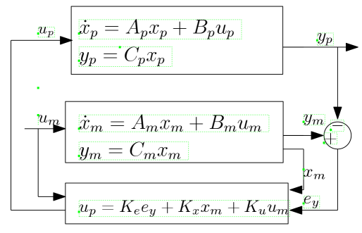
ΓpesubscriptΓ𝑝𝑒\Gamma_{pe} , ΓIesubscriptΓ𝐼𝑒\Gamma_{Ie} , ΓpxsubscriptΓ𝑝𝑥\Gamma_{px} , ΓIxsubscriptΓ𝐼𝑥\Gamma_{Ix} , ΓpusubscriptΓ𝑝𝑢\Gamma_{pu} , ΓIusubscriptΓ𝐼𝑢\Gamma_{Iu} are the time invariant weighing matrices of appropriate dimension, KIe(0)=KIe0subscript𝐾𝐼𝑒0subscript𝐾𝐼𝑒0K_{Ie}(0)=K_{Ie0} , KIx(0)=KIx0subscript𝐾𝐼𝑥0subscript𝐾𝐼𝑥0K_{Ix}(0)=K_{Ix0} , KIu(0)=KIu0subscript𝐾𝐼𝑢0subscript𝐾𝐼𝑢0K_{Iu}(0)=K_{Iu0}. σ𝜎\sigma is a positive scalar adjusted such that it does not allow the integral gain to increase without bound. The block diagram of SAC architecture is given in Fig.1.
Refer to caption
Figure 1: Block diagram of basic SAC architecture

When system output tracks the reference model output perfectly, plant state and control trajectories follow the ideal state and control trajectories, denoted by xpsuperscriptsubscript𝑥𝑝x_{p}^{*} and upsuperscriptsubscript𝑢𝑝u_{p}^{*}. The ideal state and control trajectories are

x˙p=Apxp+Bpupsuperscriptsubscript˙𝑥𝑝subscript𝐴𝑝superscriptsubscript𝑥𝑝subscript𝐵𝑝superscriptsubscript𝑢𝑝\dot{x}_{p}^{*}=A_{p}x_{p}^{*}+B_{p}u_{p}^{*} (7)
up=Kx~xm+Ku~um.superscriptsubscript𝑢𝑝~subscript𝐾𝑥subscript𝑥𝑚~subscript𝐾𝑢subscript𝑢𝑚u_{p}^{*}=\tilde{K_{x}}x_{m}+\tilde{K_{u}}u_{m}. (8)

where Kx~~subscript𝐾𝑥\tilde{K_{x}} and Ku~~subscript𝐾𝑢\tilde{K_{u}} are unknown ideal control gains. In perfect tracking case,

yp=ym=Cpxp=Cmxm.superscriptsubscript𝑦𝑝subscript𝑦𝑚subscript𝐶𝑝superscriptsubscript𝑥𝑝subscript𝐶𝑚subscript𝑥𝑚y_{p}^{*}=y_{m}=C_{p}x_{p}^{*}=C_{m}x_{m}. (9)

The error between ideal state and plant state is

ex=xpxp.subscript𝑒𝑥superscriptsubscript𝑥𝑝subscript𝑥𝑝e_{x}=x_{p}^{*}-x_{p}. (10)

Similarly the output error is

ey=CpxpCpxp=Cpex.subscript𝑒𝑦subscript𝐶𝑝superscriptsubscript𝑥𝑝subscript𝐶𝑝subscript𝑥𝑝subscript𝐶𝑝subscript𝑒𝑥e_{y}=C_{p}x_{p}^{*}-C_{p}x_{p}=C_{p}e_{x}. (11)

After deducting (1) from (7), the error differential equation is obtained as

ex˙=(ApBpK~eCp)exBp(K(t)K~)r˙subscript𝑒𝑥subscript𝐴𝑝subscript𝐵𝑝subscript~𝐾𝑒subscript𝐶𝑝subscript𝑒𝑥subscript𝐵𝑝𝐾𝑡~𝐾𝑟\dot{e_{x}}=(A_{p}-B_{p}\tilde{K}_{e}C_{p})e_{x}-B_{p}(K(t)-\tilde{K})r (12)

where K~(t)=[K~e,K~x,K~u]~𝐾𝑡subscript~𝐾𝑒subscript~𝐾𝑥subscript~𝐾𝑢\tilde{K}(t)=[\tilde{K}_{e},\tilde{K}_{x},\tilde{K}_{u}]. The following Lyapunov function is considered for stability of error dynamics.

V(t)=exTPex+trace[W((K(t)K~)Γ1(K(t)K~)T]V(t)=e_{x}^{T}Pe_{x}+trace[W((K(t)-\tilde{K})\Gamma^{-1}(K(t)-\tilde{K})^{T}] (13)

where P and Q are positive definite symmetric matrices, W is a positive definite matrix and these matrices are the solution of the following two equations.

P(ApBpK~eCp)+(ApBpK~eCp)TP=Q𝑃subscript𝐴𝑝subscript𝐵𝑝subscript~𝐾𝑒subscript𝐶𝑝superscriptsubscript𝐴𝑝subscript𝐵𝑝subscript~𝐾𝑒subscript𝐶𝑝𝑇𝑃𝑄P(A_{p}-B_{p}\tilde{K}_{e}C_{p})+(A_{p}-B_{p}\tilde{K}_{e}C_{p})^{T}P=-Q (14)
PBp=CpTWT.𝑃subscript𝐵𝑝superscriptsubscript𝐶𝑝𝑇superscript𝑊𝑇PB_{p}=C_{p}^{T}W^{T}. (15)

The conditions (14) and (15) are known as W-ASPR conditions. If the plant is minimum phase and the eigenvalues of its input output matrix product (CpBpsubscript𝐶𝑝subscript𝐵𝑝C_{p}B_{p}) are located in the right half plane, then it satisfies the W-ASPR conditions. Real world plants are not necessarily W-ASPR, but they can be made W-ASPR after augmenting them with parallel feedforward configurations (PFC). The augmented plant P(s)+D(s)𝑃𝑠𝐷𝑠P(s)+D(s) is W-ASPR if it is relative degree of zero or one, where D(s)=1C(s)𝐷𝑠1𝐶𝑠D(s)=\frac{1}{C(s)} and C(s)𝐶𝑠C(s) stabilizes the plant P(s) through feedback configuration. In the case of W-ASPR plant, the derivative of candidate Lyapunov equation (13) along the trajectory of error dynamics (12) reduces to

V˙(t)=exTQex0.˙𝑉𝑡superscriptsubscript𝑒𝑥𝑇𝑄subscript𝑒𝑥0\dot{V}(t)=-e_{x}^{T}Qe_{x}\leq 0. (16)

As the derivative of the candidate Lyapunov function is non-positive,the error dynamics is stable. In this case, V(t)𝑉𝑡V(t) is lower bounded, V˙(t)˙𝑉𝑡\dot{V}(t) is negative semi definite and V˙(t)˙𝑉𝑡\dot{V}(t) is uniformly continuous in time. There for using “Lyapunov-like lemma” slotine1991applied , it can be concluded that limtV˙(t)=0subscript𝑡˙𝑉𝑡0\displaystyle{\lim_{t\to\infty}}\dot{V}(t)=0. Hence the error between the plant and the ideal trajectory vanishes asymptotically. Therefore, Cpxp=Cpxp=Cmxmsubscript𝐶𝑝subscript𝑥𝑝subscript𝐶𝑝superscriptsubscript𝑥𝑝subscript𝐶𝑚subscript𝑥𝑚C_{p}x_{p}=C_{p}x_{p}^{*}=C_{m}x_{m}. So, the plant output follows the reference model output

3 CL-SAC architecture

The closed loop reference model gives better performance than the open loop part in MRAC architecture lavretsky2013robust ; gibson2013adaptive ; wiese2015adaptive . Closed loop reference model structure is based on the concept that driving the reference model towards the plant will reduce the control efforts required for the plant to track the reference model. The similar modification in the reference model is made in the basic SAC architecture to improve the transient performance of the original structure. In this paper, the modification of the reference model is based on the output error and it is applicable to general MIMO square systems. In CL-SAC, the reference model is not only driven by the reference signal but also by the output error between the plant and the reference model. In this case, the open loop reference model is

x˙m=Amxm+Bmum.subscript˙𝑥𝑚subscript𝐴𝑚subscript𝑥𝑚subscript𝐵𝑚subscript𝑢𝑚\dot{x}_{m}=A_{m}x_{m}+B_{m}u_{m}. (17)

The modified closed loop reference model is considered as follows

x˙mo=Amxmo+BmumLv(ymoyp)subscript˙𝑥𝑚𝑜subscript𝐴𝑚subscript𝑥𝑚𝑜subscript𝐵𝑚subscript𝑢𝑚subscript𝐿𝑣subscript𝑦𝑚𝑜subscript𝑦𝑝\dot{x}_{mo}=A_{m}x_{mo}+B_{m}u_{m}-L_{v}(y_{mo}-y_{p}) (18)
ymo=Cmxmosubscript𝑦𝑚𝑜subscript𝐶𝑚subscript𝑥𝑚𝑜y_{mo}=C_{m}x_{mo} (19)

The value of Lvsubscript𝐿𝑣L_{v} is chosen such that the reference model and subsequent error dynamics are BIBO stable. This reference model is termed as closed loop reference model and earlier reference model in equation (3)-(4) is denoted as open loop reference model. In this case output tracking error is

emy=ymoyp.subscript𝑒𝑚𝑦subscript𝑦𝑚𝑜subscript𝑦𝑝e_{my}=y_{mo}-y_{p}. (20)

The controller structure is defined similar to the basic SAC architecture, where reference model states and outputs are calculated from the modified reference model dynamics (18) and (19).

up=K(t)rsubscript𝑢𝑝𝐾𝑡𝑟u_{p}=K(t)r (21)

where,

K(t)𝐾𝑡\displaystyle K(t) =\displaystyle= [Ke(t),Kx(t),Ku(t)]subscript𝐾𝑒𝑡subscript𝐾𝑥𝑡subscript𝐾𝑢𝑡\displaystyle[K_{e}(t),K_{x}(t),K_{u}(t)]
r𝑟\displaystyle r =\displaystyle= [emy,xmo,um]superscriptsubscript𝑒𝑚𝑦subscript𝑥𝑚𝑜subscript𝑢𝑚\displaystyle[e_{my},x_{mo},u_{m}]^{\prime}
Ke(t)subscript𝐾𝑒𝑡\displaystyle K_{e}(t) =\displaystyle= Kpe(t)+KIe(t);subscript𝐾𝑝𝑒𝑡subscript𝐾𝐼𝑒𝑡\displaystyle K_{pe}(t)+K_{Ie}(t);
Kpe(t)subscript𝐾𝑝𝑒𝑡\displaystyle K_{pe}(t) =\displaystyle= emyemyTΓpe;K˙Ie(t)=emyemyTΓIeσKIesubscript𝑒𝑚𝑦superscriptsubscript𝑒𝑚𝑦𝑇subscriptΓ𝑝𝑒subscript˙𝐾𝐼𝑒𝑡subscript𝑒𝑚𝑦superscriptsubscript𝑒𝑚𝑦𝑇subscriptΓ𝐼𝑒𝜎subscript𝐾𝐼𝑒\displaystyle e_{my}e_{my}^{T}\Gamma_{pe};\quad\dot{K}_{Ie}(t)=e_{my}e_{my}^{T}\Gamma_{Ie}-\sigma K_{Ie}
Kx(t)subscript𝐾𝑥𝑡\displaystyle K_{x}(t) =\displaystyle= Kpx(t)+KIx(t);subscript𝐾𝑝𝑥𝑡subscript𝐾𝐼𝑥𝑡\displaystyle K_{px}(t)+K_{Ix}(t);
Kpx(t)subscript𝐾𝑝𝑥𝑡\displaystyle K_{px}(t) =\displaystyle= emyxmoTΓpx;K˙Ix(t)=emyxmoTΓIx;subscript𝑒𝑚𝑦superscriptsubscript𝑥𝑚𝑜𝑇subscriptΓ𝑝𝑥subscript˙𝐾𝐼𝑥𝑡subscript𝑒𝑚𝑦superscriptsubscript𝑥𝑚𝑜𝑇subscriptΓ𝐼𝑥\displaystyle e_{my}x_{mo}^{T}\Gamma_{px};\quad\dot{K}_{Ix}(t)=e_{my}x_{mo}^{T}\Gamma_{Ix};
Ku(t)subscript𝐾𝑢𝑡\displaystyle K_{u}(t) =\displaystyle= Kpu(t)+KIu(t);subscript𝐾𝑝𝑢𝑡subscript𝐾𝐼𝑢𝑡\displaystyle K_{pu}(t)+K_{Iu}(t);
Kpu(t)subscript𝐾𝑝𝑢𝑡\displaystyle K_{pu}(t) =\displaystyle= emyumTΓpu;K˙Iu(t)=emyumTΓIu.subscript𝑒𝑚𝑦superscriptsubscript𝑢𝑚𝑇subscriptΓ𝑝𝑢subscript˙𝐾𝐼𝑢𝑡subscript𝑒𝑚𝑦superscriptsubscript𝑢𝑚𝑇subscriptΓ𝐼𝑢\displaystyle e_{my}u_{m}^{T}\Gamma_{pu};\quad\dot{K}_{Iu}(t)=e_{my}u_{m}^{T}\Gamma_{Iu}.

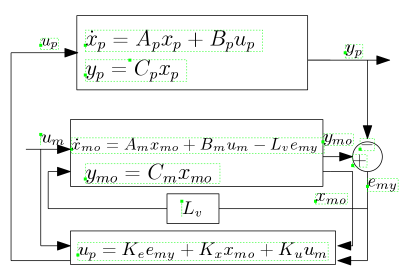
The initial conditions are kept the same as that of SAC architecture. The basic block diagram of CL-SAC architecture is given in Fig. 2 .
Refer to caption
Figure 2: Block diagram of CL-SAC architecture

3.1 Output model following

In this section, the condition for output model following for constant step input is revisited as the reference model dynamics is modified. The ideal trajectories are the linear functions of model states and model inputs.

xp=S11xmo+S12umsuperscriptsubscript𝑥𝑝subscript𝑆11subscript𝑥𝑚𝑜subscript𝑆12subscript𝑢𝑚{x}_{p}^{*}=S_{11}x_{mo}+S_{12}u_{m} (22)
up=S21xmo+S22um.superscriptsubscript𝑢𝑝subscript𝑆21subscript𝑥𝑚𝑜subscript𝑆22subscript𝑢𝑚u_{p}^{*}=S_{21}x_{mo}+S_{22}u_{m}. (23)

From (7), (9), (22) and (23) ideal trajectory dynamics can be written as,

[x˙pyp]=[ApBpCp0][S11S12S21S22][xm0um]delimited-[]superscriptsubscript˙𝑥𝑝missing-subexpressionmissing-subexpressionmissing-subexpressionmissing-subexpressionsuperscriptsubscript𝑦𝑝missing-subexpressionmissing-subexpressionmissing-subexpressiondelimited-[]subscript𝐴𝑝subscript𝐵𝑝missing-subexpressionmissing-subexpressionmissing-subexpressionsubscript𝐶𝑝0missing-subexpressionmissing-subexpressiondelimited-[]subscript𝑆11subscript𝑆12missing-subexpressionmissing-subexpressionmissing-subexpressionsubscript𝑆21subscript𝑆22missing-subexpressionmissing-subexpressiondelimited-[]subscript𝑥𝑚0missing-subexpressionmissing-subexpressionmissing-subexpressionmissing-subexpressionsubscript𝑢𝑚missing-subexpressionmissing-subexpressionmissing-subexpression\left[\begin{array}[]{cccc}\dot{x}_{p}^{*}\\ \vskip 6.0pt plus 2.0pt minus 2.0pt\cr{y}_{p}^{*}\\ \end{array}\right]=\left[\begin{array}[]{cccc}A_{p}&B_{p}\\ \vskip 6.0pt plus 2.0pt minus 2.0pt\cr C_{p}&0\\ \vskip 6.0pt plus 2.0pt minus 2.0pt\cr\end{array}\right]\left[\begin{array}[]{cccc}S_{11}&S_{12}\\ \vskip 6.0pt plus 2.0pt minus 2.0pt\cr S_{21}&S_{22}\\ \vskip 6.0pt plus 2.0pt minus 2.0pt\cr\end{array}\right]\left[\begin{array}[]{cccc}{x}_{m0}\\ \vskip 6.0pt plus 2.0pt minus 2.0pt\cr{u}_{m}\\ \end{array}\right] (24)

Let the reference command umsubscript𝑢𝑚u_{m} be restricted for a constant step input. After differentiating (22) gives

x˙p=S11x˙mosuperscriptsubscript˙𝑥𝑝subscript𝑆11subscript˙𝑥𝑚𝑜\dot{x}_{p}^{*}=S_{11}\dot{x}_{mo} (25)

as umsubscript𝑢𝑚u_{m} is considered as a constant input. Substituting the value of x˙mosubscript˙𝑥𝑚𝑜\dot{x}_{mo} from (18) in (25) gives

x˙p=S11(Amxmo+BmumLv(ymoyp))superscriptsubscript˙𝑥𝑝subscript𝑆11subscript𝐴𝑚subscript𝑥𝑚𝑜subscript𝐵𝑚subscript𝑢𝑚subscript𝐿𝑣subscript𝑦𝑚𝑜subscript𝑦𝑝\dot{x}_{p}^{*}=S_{11}(A_{m}x_{mo}+B_{m}u_{m}-L_{v}(y_{mo}-y_{p})) (26)

In perfect tracking case, ypsubscript𝑦𝑝y_{p} is denoted as ypsuperscriptsubscript𝑦𝑝{y}_{p}^{*}, then (26) can be simplified as

x˙p=(S11AmLvCm)xmo+S11Bmum+S11LvCpxpsuperscriptsubscript˙𝑥𝑝subscript𝑆11subscript𝐴𝑚subscript𝐿𝑣subscript𝐶𝑚subscript𝑥𝑚𝑜subscript𝑆11subscript𝐵𝑚subscript𝑢𝑚subscript𝑆11subscript𝐿𝑣subscript𝐶𝑝superscriptsubscript𝑥𝑝\displaystyle\dot{x}_{p}^{*}=(S_{11}A_{m}-L_{v}C_{m})x_{mo}+S_{11}B_{m}u_{m}+S_{11}L_{v}C_{p}{x}_{p}^{*} (27)

Substituting the value of xpsuperscriptsubscript𝑥𝑝{x}_{p}^{*} from (22) in (27) gives

x˙p=(S11AmLvCm+S11LvCpS11)xmo+(S11Bm\displaystyle\dot{x}_{p}^{*}=(S_{11}A_{m}-L_{v}C_{m}+S_{11}L_{v}C_{p}S_{11})x_{mo}+(S_{11}B_{m} (28)
+S11LvCpS12)um\displaystyle+S_{11}L_{v}C_{p}S_{12})u_{m}

In case of perfect tracking,

yp=ymo=Cpxp=Cmxmo.superscriptsubscript𝑦𝑝subscript𝑦𝑚𝑜subscript𝐶𝑝superscriptsubscript𝑥𝑝subscript𝐶𝑚subscript𝑥𝑚𝑜y_{p}^{*}=y_{mo}=C_{p}x_{p}^{*}=C_{m}x_{mo}. (29)

Equation(3.1) and (29) can be combined as

[x˙pyp]=[S11AmLvCm+S11LvCpS11S11Bm+S11LvCpS12Cm0]delimited-[]superscriptsubscript˙𝑥𝑝missing-subexpressionmissing-subexpressionmissing-subexpressionmissing-subexpressionsuperscriptsubscript𝑦𝑝missing-subexpressionmissing-subexpressionmissing-subexpressiondelimited-[]subscript𝑆11subscript𝐴𝑚subscript𝐿𝑣subscript𝐶𝑚subscript𝑆11subscript𝐿𝑣subscript𝐶𝑝subscript𝑆11subscript𝑆11subscript𝐵𝑚subscript𝑆11subscript𝐿𝑣subscript𝐶𝑝subscript𝑆12missing-subexpressionmissing-subexpressionmissing-subexpressionsubscript𝐶𝑚0missing-subexpressionmissing-subexpression\left[\begin{array}[]{cccc}\dot{x}_{p}^{*}\\ \vskip 6.0pt plus 2.0pt minus 2.0pt\cr{y}_{p}^{*}\\ \end{array}\right]=\left[\begin{array}[]{cccc}S_{11}A_{m}-L_{v}C_{m}+S_{11}L_{v}C_{p}S_{11}&S_{11}B_{m}+S_{11}L_{v}C_{p}S_{12}\\ \vskip 6.0pt plus 2.0pt minus 2.0pt\cr C_{m}&0\\ \vskip 6.0pt plus 2.0pt minus 2.0pt\cr\end{array}\right] (30)

From (24) and (30), (30) can be written as

[S11AmLvCm+S11LvCpS11S11Bm+S11LvCpS12Cm0]delimited-[]subscript𝑆11subscript𝐴𝑚subscript𝐿𝑣subscript𝐶𝑚subscript𝑆11subscript𝐿𝑣subscript𝐶𝑝subscript𝑆11subscript𝑆11subscript𝐵𝑚subscript𝑆11subscript𝐿𝑣subscript𝐶𝑝subscript𝑆12missing-subexpressionmissing-subexpressionmissing-subexpressionsubscript𝐶𝑚0missing-subexpressionmissing-subexpression\displaystyle\left[\begin{array}[]{cccc}S_{11}A_{m}-L_{v}C_{m}+S_{11}L_{v}C_{p}S_{11}&S_{11}B_{m}+S_{11}L_{v}C_{p}S_{12}\\ \vskip 6.0pt plus 2.0pt minus 2.0pt\cr C_{m}&0\\ \vskip 6.0pt plus 2.0pt minus 2.0pt\cr\end{array}\right]
=[ApBpCp0][S11S12S21S22]absentdelimited-[]subscript𝐴𝑝subscript𝐵𝑝missing-subexpressionmissing-subexpressionmissing-subexpressionsubscript𝐶𝑝0missing-subexpressionmissing-subexpressiondelimited-[]subscript𝑆11subscript𝑆12missing-subexpressionmissing-subexpressionmissing-subexpressionsubscript𝑆21subscript𝑆22missing-subexpressionmissing-subexpression\displaystyle=\left[\begin{array}[]{cccc}A_{p}&B_{p}\\ \vskip 6.0pt plus 2.0pt minus 2.0pt\cr C_{p}&0\\ \vskip 6.0pt plus 2.0pt minus 2.0pt\cr\end{array}\right]\left[\begin{array}[]{cccc}S_{11}&S_{12}\\ \vskip 6.0pt plus 2.0pt minus 2.0pt\cr S_{21}&S_{22}\\ \vskip 6.0pt plus 2.0pt minus 2.0pt\cr\end{array}\right]

The solution of the above matrix equation exist as there are (np+m)(nm+mm)subscript𝑛𝑝𝑚subscript𝑛𝑚subscript𝑚𝑚(n_{p}+m)(n_{m}+m_{m}) number of equations as well as unknowns. This implies that perfect tracking in the case of constant step input is possible in case of modified architecture.
If the reference command is generated from the following differential equation,

v˙m=Avvm;um=cvvmformulae-sequencesubscript˙𝑣𝑚subscript𝐴𝑣subscript𝑣𝑚subscript𝑢𝑚subscript𝑐𝑣subscript𝑣𝑚\dot{v}_{m}=A_{v}v_{m};\quad u_{m}=c_{v}v_{m} (33)

the perfect tracking is expected for following conditions

dim(xm)+dim(um)dim(vm).𝑑𝑖𝑚subscript𝑥𝑚𝑑𝑖𝑚subscript𝑢𝑚𝑑𝑖𝑚subscript𝑣𝑚dim(x_{m})+dim(u_{m})\geq dim(v_{m}). (34)

In case of general tracking command, it can be shown that CL-SAC architecture follows the reference command with bounded tracking error.

3.2 Stability analysis

In this section, we analyze the stability of the system since the reference model dynamics is modified.This modification in the reference model does not affect the error dynamics (12).

ex=xpxpsubscript𝑒𝑥superscriptsubscript𝑥𝑝subscript𝑥𝑝e_{x}=x_{p}^{*}-x_{p} (35)
ex˙=(ApBpK~eCp)exBp(K(t)K~)r˙subscript𝑒𝑥subscript𝐴𝑝subscript𝐵𝑝subscript~𝐾𝑒subscript𝐶𝑝subscript𝑒𝑥subscript𝐵𝑝𝐾𝑡~𝐾𝑟\dot{e_{x}}=(A_{p}-B_{p}\tilde{K}_{e}C_{p})e_{x}-B_{p}(K(t)-\tilde{K})r (36)

Hence, it can be shown that the error between plant and ideal state trajectory goes down asymptotically. Therefore, the output error between plant and closed loop reference model goes to zero, and hence, the closed loop model reduces to open loop reference model asymptotically. So, the plant output is able to track the reference model output.

The effect of the modified architecture is visible in output error dynamics between the plant output and the reference model output. This is discussed in details in the next section.

4 Performance analysis

In the case of SAC architecture, the error dynamics between the plant output and the reference model output is obtained as follows:

ey˙=Cmx˙mCpx˙p.˙subscript𝑒𝑦subscript𝐶𝑚subscript˙𝑥𝑚subscript𝐶𝑝subscript˙𝑥𝑝\dot{e_{y}}=C_{m}\dot{x}_{m}-C_{p}\dot{x}_{p}. (37)

Using the value of x˙msubscript˙𝑥𝑚\dot{x}_{m} and x˙psubscript˙𝑥𝑝\dot{x}_{p} from (3) and (1) respectively in (37); we get

ey˙=Cm(Amxm+Bmum)Cp(Apxp+Bpup)˙subscript𝑒𝑦subscript𝐶𝑚subscript𝐴𝑚subscript𝑥𝑚subscript𝐵𝑚subscript𝑢𝑚subscript𝐶𝑝subscript𝐴𝑝subscript𝑥𝑝subscript𝐵𝑝subscript𝑢𝑝\dot{e_{y}}=C_{m}(A_{m}x_{m}+B_{m}u_{m})-C_{p}(A_{p}x_{p}+B_{p}u_{p}) (38)

Putting the value of upsubscript𝑢𝑝u_{p} as per (6) in (38), we get

ey˙=Cm(Amxm+Bmum)Cp(Apx+Bp(Ke(t)ey\displaystyle\dot{e_{y}}=C_{m}(A_{m}x_{m}+B_{m}u_{m})-C_{p}(A_{p}x+B_{p}(K_{e}(t)e_{y} (39)
+Kx(t)xm+Kuum)\displaystyle+K_{x}(t)x_{m}+K_{u}u_{m}) (40)

Finally, we get

ey˙=Ammey+θ~T(t)ω˙subscript𝑒𝑦subscript𝐴𝑚𝑚subscript𝑒𝑦superscript~𝜃𝑇𝑡𝜔\dot{e_{y}}=A_{mm}e_{y}+\tilde{\theta}^{T}(t)\omega (41)

where Amm=CpBpKesubscript𝐴𝑚𝑚subscript𝐶𝑝subscript𝐵𝑝subscript𝐾𝑒A_{mm}=-C_{p}B_{p}K_{e},
θ~T(t)=[CpAp,CmAmCpBpKx(t),CmBmCpBpKu(t)]superscript~𝜃𝑇𝑡subscript𝐶𝑝subscript𝐴𝑝subscript𝐶𝑚subscript𝐴𝑚subscript𝐶𝑝subscript𝐵𝑝subscript𝐾𝑥𝑡subscript𝐶𝑚subscript𝐵𝑚subscript𝐶𝑝subscript𝐵𝑝subscript𝐾𝑢𝑡\tilde{\theta}^{T}(t)=[-C_{p}A_{p},C_{m}A_{m}-C_{p}B_{p}K_{x}(t),C_{m}B_{m}-C_{p}B_{p}K_{u}(t)] and ω=[xp,xm,um]T𝜔superscriptsubscript𝑥𝑝subscript𝑥𝑚subscript𝑢𝑚𝑇\omega=[x_{p},x_{m},u_{m}]^{T}.

In the case of CL-SAC architecture, the output tracking error is emysubscript𝑒𝑚𝑦e_{my} and the error dynamics is

emy˙=Cm(Amxmo+BmumLv(ymoyp))Cp(Apxp+Bpup).˙subscript𝑒𝑚𝑦subscript𝐶𝑚subscript𝐴𝑚subscript𝑥𝑚𝑜subscript𝐵𝑚subscript𝑢𝑚subscript𝐿𝑣subscript𝑦𝑚𝑜subscript𝑦𝑝subscript𝐶𝑝subscript𝐴𝑝subscript𝑥𝑝subscript𝐵𝑝subscript𝑢𝑝\dot{e_{my}}=C_{m}(A_{m}x_{mo}+B_{m}u_{m}-L_{v}(y_{mo}-y_{p}))-C_{p}(A_{p}x_{p}+B_{p}u_{p}). (42)

Equation (42) can be written as:

emy˙=Amnemy+θ~T(t)ω˙subscript𝑒𝑚𝑦subscript𝐴𝑚𝑛subscript𝑒𝑚𝑦superscript~𝜃𝑇𝑡𝜔\dot{e_{my}}=A_{mn}e_{my}+\tilde{\theta}^{T}(t)\omega (43)

where Amn=CpBpKeCmLvsubscript𝐴𝑚𝑛subscript𝐶𝑝subscript𝐵𝑝subscript𝐾𝑒subscript𝐶𝑚subscript𝐿𝑣A_{mn}=-C_{p}B_{p}K_{e}-C_{m}L_{v},

θ~T(t)=[CpAp,CmAmCpBpKx(t),CmBmCpBpKu(t)]superscript~𝜃𝑇𝑡subscript𝐶𝑝subscript𝐴𝑝subscript𝐶𝑚subscript𝐴𝑚subscript𝐶𝑝subscript𝐵𝑝subscript𝐾𝑥𝑡subscript𝐶𝑚subscript𝐵𝑚subscript𝐶𝑝subscript𝐵𝑝subscript𝐾𝑢𝑡\tilde{\theta}^{T}(t)=[-C_{p}A_{p},C_{m}A_{m}-C_{p}B_{p}K_{x}(t),C_{m}B_{m}-C_{p}B_{p}K_{u}(t)] and ω=[xp,xmo,um]T𝜔superscriptsubscript𝑥𝑝subscript𝑥𝑚𝑜subscript𝑢𝑚𝑇\omega=[x_{p},x_{mo},u_{m}]^{T}.

The plant is able to do bounded tracking of the output of the reference model, so the output error dynamics is stable.
In the case of SAC architecture, since the output error dynamics is stable; there exist a Lyapunov function V(t) whose derivative along the trajectories of the system in (41) is negative semi-definite:

V˙(t)=eyTQ1ey0˙𝑉𝑡superscriptsubscript𝑒𝑦𝑇subscript𝑄1subscript𝑒𝑦0\dot{V}(t)=-e_{y}^{T}Q_{1}e_{y}\leq 0 (44)

where Q1=Q1T>0subscript𝑄1superscriptsubscript𝑄1𝑇0Q_{1}=Q_{1}^{T}>0. Let’s consider this Lyapunov function in following form

V(t)=eyTP1ey+f(θ~(t),Γ)𝑉𝑡superscriptsubscript𝑒𝑦𝑇subscript𝑃1subscript𝑒𝑦𝑓~𝜃𝑡ΓV(t)=e_{y}^{T}P_{1}e_{y}+f(\tilde{\theta}(t),\Gamma) (45)

where ΓΓ\Gamma represent the set of gains ΓIx,ΓIesubscriptΓ𝐼𝑥subscriptΓ𝐼𝑒\Gamma_{Ix},\Gamma_{Ie} etc and P1=P1T>0subscript𝑃1superscriptsubscript𝑃1𝑇0P_{1}=P_{1}^{T}>0 is the solution of the following Algebraic Riccati equation.

P1Amm+AmmTP1=Q1subscript𝑃1subscript𝐴𝑚𝑚superscriptsubscript𝐴𝑚𝑚𝑇subscript𝑃1subscript𝑄1P_{1}A_{mm}+A_{mm}^{T}P_{1}=-Q_{1} (46)

Since, V˙(t)0˙𝑉𝑡0\dot{V}(t)\leq 0;

ey2V(t)λmin(P1)V(0)λmin(P1)superscriptnormsubscript𝑒𝑦2𝑉𝑡subscript𝜆𝑚𝑖𝑛subscript𝑃1𝑉0subscript𝜆𝑚𝑖𝑛subscript𝑃1\parallel e_{y}\parallel^{2}\leq\frac{V(t)}{\lambda_{min}(P_{1})}\leq\frac{V(0)}{\lambda_{min}(P_{1})} (47)

where λmin(P1)subscript𝜆𝑚𝑖𝑛subscript𝑃1\lambda_{min}(P_{1}) is minimum eigenvalue value of P1subscript𝑃1P_{1}. Since the error dynamics is bounded, f(θ~(t))𝑓~𝜃𝑡f(\tilde{\theta}(t)) is bounded by positive constant C𝐶C. So, bound for V(t) can be written as;

V(t)eyTP1ey+C𝑉𝑡superscriptsubscript𝑒𝑦𝑇subscript𝑃1subscript𝑒𝑦𝐶V(t)\leq e_{y}^{T}P_{1}e_{y}+C (48)

We have the following inequality,
eyTQ1eyeyTλmin(Q1)eyλmin(Q1)λmax(P1)eyTλmax(P1)eysuperscriptsubscript𝑒𝑦𝑇subscript𝑄1subscript𝑒𝑦superscriptsubscript𝑒𝑦𝑇subscript𝜆𝑚𝑖𝑛subscript𝑄1subscript𝑒𝑦subscript𝜆𝑚𝑖𝑛subscript𝑄1subscript𝜆𝑚𝑎𝑥subscript𝑃1superscriptsubscript𝑒𝑦𝑇subscript𝜆𝑚𝑎𝑥subscript𝑃1subscript𝑒𝑦e_{y}^{T}Q_{1}e_{y}\geq e_{y}^{T}\lambda_{min}(Q_{1})e_{y}\geq\frac{\lambda_{min}(Q_{1})}{\lambda_{max}(P_{1})}e_{y}^{T}\lambda_{max}(P_{1})e_{y}

Further,
λmin(Q1)λmax(P1)eyTλmax(P1)eyλmin(Q1)λmax(P1)eyTP1ey=γ(eyTP1ey)subscript𝜆𝑚𝑖𝑛subscript𝑄1subscript𝜆𝑚𝑎𝑥subscript𝑃1superscriptsubscript𝑒𝑦𝑇subscript𝜆𝑚𝑎𝑥subscript𝑃1subscript𝑒𝑦subscript𝜆𝑚𝑖𝑛subscript𝑄1subscript𝜆𝑚𝑎𝑥subscript𝑃1superscriptsubscript𝑒𝑦𝑇subscript𝑃1subscript𝑒𝑦𝛾superscriptsubscript𝑒𝑦𝑇subscript𝑃1subscript𝑒𝑦\frac{\lambda_{min}(Q_{1})}{\lambda_{max}(P_{1})}e_{y}^{T}\lambda_{max}(P_{1})e_{y}\geq\frac{\lambda_{min}(Q_{1})}{\lambda_{max}(P_{1})}e_{y}^{T}P_{1}e_{y}=\gamma(e_{y}^{T}P_{1}e_{y})
where γ=λmin(Q1)λmax(P1)𝛾subscript𝜆𝑚𝑖𝑛subscript𝑄1subscript𝜆𝑚𝑎𝑥subscript𝑃1\gamma=\frac{\lambda_{min}(Q_{1})}{\lambda_{max}(P_{1})}. Therefore,

V˙(t)=eyTQ1eyγ(eyTP1ey).˙𝑉𝑡superscriptsubscript𝑒𝑦𝑇subscript𝑄1subscript𝑒𝑦𝛾superscriptsubscript𝑒𝑦𝑇subscript𝑃1subscript𝑒𝑦\dot{V}(t)=-e_{y}^{T}Q_{1}e_{y}\leq-\gamma(e_{y}^{T}P_{1}e_{y}). (49)

Using the value of eyTP1eysuperscriptsubscript𝑒𝑦𝑇subscript𝑃1subscript𝑒𝑦e_{y}^{T}P_{1}e_{y} from (48) in (49) gives

V˙(t)+γV(t)γC.˙𝑉𝑡𝛾𝑉𝑡𝛾𝐶\dot{V}(t)+\gamma V(t)\leq\gamma C. (50)

After integration of V˙(t)˙𝑉𝑡\dot{V}(t) we get,

V(t)V(0)eγt+CCeγt.𝑉𝑡𝑉0superscript𝑒𝛾𝑡𝐶𝐶superscript𝑒𝛾𝑡V(t)\leq V(0)e^{-\gamma t}+C-Ce^{-\gamma t}. (51)

From (48), it follows that

V(0)CeyT(0)P1ey(0).𝑉0𝐶superscriptsubscript𝑒𝑦𝑇0subscript𝑃1subscript𝑒𝑦0V(0)-C\leq e_{y}^{T}(0)P_{1}e_{y}(0). (52)

Therefore V(t)𝑉𝑡V(t) is upper bounded as

V(t)C+eyT(0)P1ey(0)eγt.𝑉𝑡𝐶superscriptsubscript𝑒𝑦𝑇0subscript𝑃1subscript𝑒𝑦0superscript𝑒𝛾𝑡V(t)\leq C+e_{y}^{T}(0)P_{1}e_{y}(0)e^{-\gamma t}. (53)

Considering (47), the output error has the following upper bound:

ey(λmin(P1))1(C+eyT(0)P1ey(0)eγt)normsubscript𝑒𝑦superscriptsubscript𝜆𝑚𝑖𝑛subscript𝑃11𝐶superscriptsubscript𝑒𝑦𝑇0subscript𝑃1subscript𝑒𝑦0superscript𝑒𝛾𝑡\parallel e_{y}\parallel\leq\sqrt{(\lambda_{min}(P_{1}))^{-1}(C+e_{y}^{T}(0)P_{1}e_{y}(0)e^{-\gamma t})} (54)

One part of the above bound is due to initialization error between the plant output and the reference model output, this term decays exponentially. If initialization is done perfectly, this output error bound reduces to,

eyC(λmin(P1))1.normsubscript𝑒𝑦𝐶superscriptsubscript𝜆𝑚𝑖𝑛subscript𝑃11\parallel e_{y}\parallel\leq\sqrt{C(\lambda_{min}(P_{1}))^{-1}}. (55)

λmin(P1)subscript𝜆𝑚𝑖𝑛subscript𝑃1\lambda_{min}(P_{1}) satisfies the following inequality yasuda1979upper :

λmin(P1)2λmax1(S1)subscript𝜆𝑚𝑖𝑛subscript𝑃12superscriptsubscript𝜆𝑚𝑎𝑥1subscript𝑆1\lambda_{min}(P_{1})\geq 2\lambda_{max}^{-1}(S_{1}) (56)

where S1=(Amm+AmmT)Q11/2subscript𝑆1subscript𝐴𝑚𝑚superscriptsubscript𝐴𝑚𝑚𝑇superscriptsubscript𝑄112S_{1}=-(A_{mm}+A_{mm}^{T})Q_{1}^{-1}/2 and λmax(S1)subscript𝜆𝑚𝑎𝑥subscript𝑆1\lambda_{max}(S_{1}) is the maximum eigenvalue of S1subscript𝑆1S_{1}.

Therefore, the output error satisfy the following bound:

eyβλmax(S1)normsubscript𝑒𝑦𝛽subscript𝜆𝑚𝑎𝑥subscript𝑆1\parallel e_{y}\parallel\leq\beta\sqrt{\lambda_{max}(S_{1})} (57)

where β𝛽\beta is constant depends on value of C. The similar bound for the CL-SAC architecture is

emyβλmax(S2)normsubscript𝑒𝑚𝑦𝛽subscript𝜆𝑚𝑎𝑥subscript𝑆2\parallel e_{my}\parallel\leq\beta\sqrt{\lambda_{max}(S_{2})} (58)

where S2=(Amn+AmnT)Q21/2subscript𝑆2subscript𝐴𝑚𝑛superscriptsubscript𝐴𝑚𝑛𝑇superscriptsubscript𝑄212S_{2}=-(A_{mn}+A_{mn}^{T})Q_{2}^{-1}/2.
Let Q1=Q2subscript𝑄1subscript𝑄2Q_{1}=Q_{2} is chosen as Identity matrix.
λmax(S2)=λmax([(Amm+AmmT)CmLv(CmLv)T])subscript𝜆𝑚𝑎𝑥subscript𝑆2subscript𝜆𝑚𝑎𝑥delimited-[]subscript𝐴𝑚𝑚superscriptsubscript𝐴𝑚𝑚𝑇subscript𝐶𝑚subscript𝐿𝑣superscriptsubscript𝐶𝑚subscript𝐿𝑣𝑇\lambda_{max}(S_{2})=\lambda_{max}(-[(A_{mm}+A_{mm}^{T})-C_{m}L_{v}-(C_{m}L_{v})^{T}])
Clearly with proper choice of Lvsubscript𝐿𝑣L_{v}, λmax(S2\lambda_{max}(S_{2}) can be made smaller than the λmax(S1\lambda_{max}(S_{1}). Therefore, the bound of emysubscript𝑒𝑚𝑦e_{my} can be made tighter than the eysubscript𝑒𝑦e_{y}. Hence, in CL-SAC architecture output tracking error can be made further smaller than SAC architecture, which will improve the transient performance.

4.1 Selection of Lvsubscript𝐿𝑣L_{v}

In gibson2013adaptive , some guidelines are available for design of the gain of the error feedback term for the case of MRAC structure. In the case of SAC structure similar analysis is performed. A simplified analysis is done for scalar reference model, i.e the dimension of nm,mm,msubscript𝑛𝑚subscript𝑚𝑚𝑚n_{m},m_{m},m is one. The response of the open loop reference model in (17) with initial conditions xm(0)=x(0)subscript𝑥𝑚0𝑥0x_{m}(0)=x(0) is

xm(t)=eAmtx(0)+0teAm(tτ)Bmum(τ)𝑑τsubscript𝑥𝑚𝑡superscript𝑒subscript𝐴𝑚𝑡𝑥0superscriptsubscript0𝑡superscript𝑒subscript𝐴𝑚𝑡𝜏subscript𝐵𝑚subscript𝑢𝑚𝜏differential-d𝜏x_{m}(t)=e^{A_{m}t}x(0)+\int_{0}^{t}e^{A_{m}(t-\tau)}B_{m}u_{m}(\tau)d\tau (59)

The response of the closed loop reference model in (18) with same initial condition as xmo(0)=x(0)subscript𝑥𝑚𝑜0𝑥0x_{mo}(0)=x(0) is

xmo(t)=eAmtx(0)+0teAm(tτ)Bmum(τ)𝑑τsubscript𝑥𝑚𝑜𝑡superscript𝑒subscript𝐴𝑚𝑡𝑥0superscriptsubscript0𝑡superscript𝑒subscript𝐴𝑚𝑡𝜏subscript𝐵𝑚subscript𝑢𝑚𝜏differential-d𝜏\displaystyle x_{mo}(t)=e^{A_{m}t}x(0)+\int_{0}^{t}e^{A_{m}(t-\tau)}B_{m}u_{m}(\tau)d\tau (60)
Lv0teAm(tτ)emy(τ)𝑑τsubscript𝐿𝑣superscriptsubscript0𝑡superscript𝑒subscript𝐴𝑚𝑡𝜏subscript𝑒𝑚𝑦𝜏differential-d𝜏\displaystyle-L_{v}\int_{0}^{t}e^{A_{m}(t-\tau)}e_{my}(\tau)d\tau

The difference of response between closed loop reference model in (18) and the open loop reference model in (17) having same initial conditions can be written as

xmo(t)=xmo(t)xm(t)=Lv0teAm(tτ)emy(τ)𝑑τsubscript𝑥𝑚𝑜𝑡subscript𝑥𝑚𝑜𝑡subscript𝑥𝑚𝑡subscript𝐿𝑣superscriptsubscript0𝑡superscript𝑒subscript𝐴𝑚𝑡𝜏subscript𝑒𝑚𝑦𝜏differential-d𝜏\bigtriangleup x_{mo}(t)=x_{mo}(t)-x_{m}(t)=-L_{v}\int_{0}^{t}e^{A_{m}(t-\tau)}e_{my}(\tau)d\tau (61)

Applying Cauchy Schwartz inequality;

0teAm(tτ)emy(τ)𝑑τ0t(eAm(tτ))2𝑑τ0t(emy(τ))2𝑑τsuperscriptsubscript0𝑡superscript𝑒subscript𝐴𝑚𝑡𝜏subscript𝑒𝑚𝑦𝜏differential-d𝜏superscriptsubscript0𝑡superscriptsuperscript𝑒subscript𝐴𝑚𝑡𝜏2differential-d𝜏superscriptsubscript0𝑡superscriptsubscript𝑒𝑚𝑦𝜏2differential-d𝜏\int_{0}^{t}e^{A_{m}(t-\tau)}e_{my}(\tau)d\tau\leq\sqrt{\int_{0}^{t}(e^{A_{m}(t-\tau)})^{2}d\tau}\sqrt{\int_{0}^{t}(e_{my}(\tau))^{2}d\tau} (62)

We have,

0t(eAm(tτ))2𝑑τ12Amsuperscriptsubscript0𝑡superscriptsuperscript𝑒subscript𝐴𝑚𝑡𝜏2differential-d𝜏1norm2subscript𝐴𝑚\int_{0}^{t}(e^{A_{m}(t-\tau)})^{2}d\tau\leq\frac{1}{\parallel 2A_{m}\parallel} (63)

Also,

0t(emy(τ))2𝑑τV(0)λmin(P1)superscriptsubscript0𝑡superscriptsubscript𝑒𝑚𝑦𝜏2differential-d𝜏𝑉0subscript𝜆𝑚𝑖𝑛subscript𝑃1\int_{0}^{t}(e_{my}(\tau))^{2}d\tau\leq\frac{V(0)}{\lambda_{min}(P_{1})} (64)

Using the inequalities in (63) and (64), the inequality in (62) can be simplified as,

xmo(t)Lv12AmV(0)λmin(P1)subscript𝑥𝑚𝑜𝑡normsubscript𝐿𝑣1norm2subscript𝐴𝑚𝑉0subscript𝜆𝑚𝑖𝑛subscript𝑃1\bigtriangleup x_{mo}(t)\leq\parallel L_{v}\parallel\sqrt{\frac{1}{\parallel 2A_{m}\parallel}}\sqrt{\frac{V(0)}{\lambda_{min}(P_{1})}} (65)

Equivalently,

xmo(t)Lv12Amey(0)TP1ey(0)+f(θ~(0),Γ)λmin(P1)subscript𝑥𝑚𝑜𝑡normsubscript𝐿𝑣1norm2subscript𝐴𝑚subscript𝑒𝑦superscript0𝑇subscript𝑃1subscript𝑒𝑦0𝑓~𝜃0Γsubscript𝜆𝑚𝑖𝑛subscript𝑃1\bigtriangleup x_{mo}(t)\leq\parallel L_{v}\parallel\sqrt{\frac{1}{\parallel 2A_{m}\parallel}}\sqrt{\frac{e_{y}(0)^{T}P_{1}e_{y}(0)+f(\tilde{\theta}(0),\Gamma)}{\lambda_{min}(P_{1})}} (66)

The value of Lvsubscript𝐿𝑣L_{v} is chosen such that the reference model dynamics and subsequent error dynamics is BIBO stable. Clearly from the bound of xmo(t)subscript𝑥𝑚𝑜𝑡\bigtriangleup x_{mo}(t); the high value of Lvsubscript𝐿𝑣L_{v} will make the xmo(t)subscript𝑥𝑚𝑜𝑡\bigtriangleup x_{mo}(t) large, i.e, the response of closed loop reference model will deviate more from the response of open loop reference model. Also, The low value of Lvsubscript𝐿𝑣L_{v} will reduce the effect of error feedback in the reference model dynamics. The value of Lvsubscript𝐿𝑣L_{v} needs to be selected as a function of ΓΓ\Gamma optimally to balance both the effects. Mathematically, it can be shown that a high value of Lvsubscript𝐿𝑣L_{v} will reduce the oscillation in the control signal. In general, if the magnitude of Lvsubscript𝐿𝑣L_{v} is selected as high as possible and closer to the value of ΓΓ\Gamma, the advantage of Lvsubscript𝐿𝑣L_{v} can be obtained.

5 Simulation

MAV lateral dynamics are considered to verify the improvement in the new architecture. MAV lateral states are lateral velocity (v), roll rate (p), yaw rate (r), roll attitude (ϕ)italic-ϕ(\phi). Generally, in MAV case, roll rate and yaw rate are available form the gyroscope sensor and the (ϕ)italic-ϕ(\phi) is estimated from the estimation loop. The lateral dynamics need to track the roll attitude command from the guidance loop. Therefore, the plant output ypsubscript𝑦𝑝y_{p} (ϕ)italic-ϕ(\phi) has to track the output of the reference model which is driven by the commanded roll angle (ϕcmd)\phi_{cmd}). The roll rate and yaw rate can be feedback to increase the damping in the inner loop. Here, we will consider the tracking and stabilization problem only using the attitude (ϕ)italic-ϕ(\phi).

5.1 Lateral dynamics-Roll attitude tracking

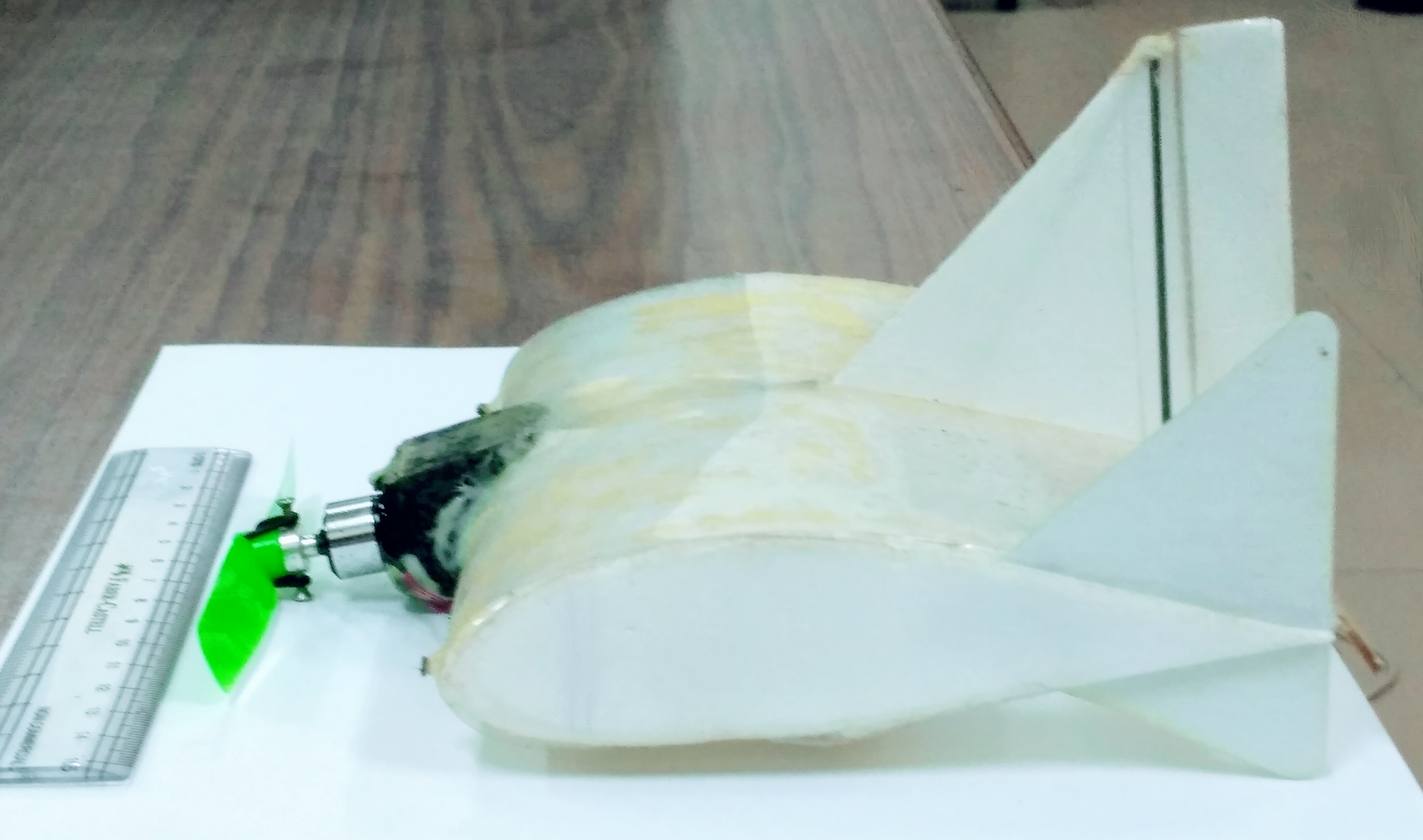
The lateral model of 150 mm KH2013A MAV is considered for simulation harikumar2016nonlinear . The photograph of KH2013A MAV is shown in Fig.3. In this MAV, the lateral control is done by rudder input(δrsubscript𝛿𝑟\delta_{r}). The states, control and output variable are as follows:
xp=[v,p,r,ϕ];subscript𝑥𝑝superscript𝑣𝑝𝑟italic-ϕx_{p}=[v,p,r,\phi]^{\prime};     up=δrsubscript𝑢𝑝subscript𝛿𝑟u_{p}=\delta_{r};    yp=ϕsubscript𝑦𝑝italic-ϕy_{p}=\phi.
The state matrix, control matrix, output matrix are as follows:
Alp=[3.341.937.557.8240.52.222.480.0234.02.8427.00.00.01.00.2680.0]subscript𝐴𝑙𝑝delimited-[]3.341.937.557.82missing-subexpression40.52.222.480.0missing-subexpression234.02.8427.00.0missing-subexpression0.01.00.2680.0A_{lp}=\left[\begin{array}[]{cccc}-3.34&1.93&-7.55&7.82\\ \vskip 6.0pt plus 2.0pt minus 2.0pt\cr-40.5&-2.22&2.48&0.0\\ \vskip 6.0pt plus 2.0pt minus 2.0pt\cr 234.0&-2.84&-27.0&0.0\\ \vskip 6.0pt plus 2.0pt minus 2.0pt\cr 0.0&1.0&0.268&0.0\end{array}\right]
Blp=[8.41,59.7,793.0,0.0]subscript𝐵𝑙𝑝superscript8.4159.7793.00.0B_{lp}=[-8.41,59.7,793.0,0.0]^{\prime};  Clp=[0,0,0,1]subscript𝐶𝑙𝑝0001C_{lp}=[0,0,0,1]

Refer to caption
Figure 3: Photograph of KH2013A MAV

The available actuator bandwidth in case of MAV is limited due to restriction on weight and power budget. The actuator dynamics is considered as:

[δ˙rδ¨r]=[01236772.22][δrδ˙r]+[02367]δcommanddelimited-[]subscript˙𝛿𝑟missing-subexpressionmissing-subexpressionmissing-subexpressionmissing-subexpressionsubscript¨𝛿𝑟missing-subexpressionmissing-subexpressionmissing-subexpressiondelimited-[]01missing-subexpressionmissing-subexpressionmissing-subexpression236772.22missing-subexpressionmissing-subexpressiondelimited-[]subscript𝛿𝑟missing-subexpressionmissing-subexpressionmissing-subexpressionmissing-subexpressionsubscript˙𝛿𝑟missing-subexpressionmissing-subexpressionmissing-subexpressiondelimited-[]0missing-subexpressionmissing-subexpressionmissing-subexpressionmissing-subexpression2367missing-subexpressionmissing-subexpressionmissing-subexpressionsubscript𝛿𝑐𝑜𝑚𝑚𝑎𝑛𝑑\left[\begin{array}[]{cccc}\dot{\delta}_{r}\\ \vskip 6.0pt plus 2.0pt minus 2.0pt\cr\ddot{\delta}_{r}\\ \end{array}\right]=\left[\begin{array}[]{cccc}0&1\\ \vskip 6.0pt plus 2.0pt minus 2.0pt\cr-2367&-72.22\\ \vskip 6.0pt plus 2.0pt minus 2.0pt\cr\end{array}\right]\left[\begin{array}[]{cccc}{\delta}_{r}\\ \vskip 6.0pt plus 2.0pt minus 2.0pt\cr\dot{\delta}_{r}\\ \vskip 6.0pt plus 2.0pt minus 2.0pt\cr\end{array}\right]+\left[\begin{array}[]{cccc}0\\ \vskip 6.0pt plus 2.0pt minus 2.0pt\cr 2367\\ \end{array}\right]{\delta}_{command} (67)

The augmented model of the plant with actuator dynamics of (67) is as follows:
States, control and output variable are xp=[v,p,r,ϕ,δr,δ˙r],subscript𝑥𝑝superscript𝑣𝑝𝑟italic-ϕsubscript𝛿𝑟subscript˙𝛿𝑟x_{p}=[v,p,r,\phi,\delta_{r},\dot{\delta}_{r}]^{\prime}, up=δcommandsubscript𝑢𝑝subscript𝛿𝑐𝑜𝑚𝑚𝑎𝑛𝑑u_{p}=\delta_{command}, yp=ϕsubscript𝑦𝑝italic-ϕy_{p}=\phi.
The augmented state, control and output matrix are
Ap=[3.341.937.557.828.41040.52.222.480.059.70234.02.8427.00.0793.000.01.00.2680.0000.0000.0010.0000.0236772.22],subscript𝐴𝑝delimited-[]3.341.937.557.828.410missing-subexpression40.52.222.480.059.70missing-subexpression234.02.8427.00.0793.00missing-subexpression0.01.00.2680.000missing-subexpression0.0000.001missing-subexpression0.0000.0236772.22A_{p}=\left[\begin{array}[]{cccccc}-3.34&1.93&-7.55&7.82&-8.41&0\\ \vskip 6.0pt plus 2.0pt minus 2.0pt\cr-40.5&-2.22&2.48&0.0&59.7&0\\ \vskip 6.0pt plus 2.0pt minus 2.0pt\cr 234.0&-2.84&-27.0&0.0&793.0&0\\ \vskip 6.0pt plus 2.0pt minus 2.0pt\cr 0.0&1.0&0.268&0.0&0&0\\ \vskip 6.0pt plus 2.0pt minus 2.0pt\cr 0.0&0&0&0.0&0&1\\ \vskip 6.0pt plus 2.0pt minus 2.0pt\cr 0.0&0&0&0.0&-2367&-72.22\\ \end{array}\right],
Bp=[0,0,0,0,0,2367]subscript𝐵𝑝superscript000002367B_{p}=[0,0,0,0,0,2367]^{\prime};     Cp=[0,0,0,1,0,0]subscript𝐶𝑝000100C_{p}=[0,0,0,1,0,0].

In this case, plant output ϕitalic-ϕ\phi needs to track a single command ϕcmdsubscriptitalic-ϕ𝑐𝑚𝑑\phi_{cmd} using a single control input δrsubscript𝛿𝑟\delta_{r}. So, this tracking problem fits perfectly for SAC architecture.
A first order BIBO stable simple reference model is considered. In case of SAC, the following reference model is considered.
x˙m=5xm+5ϕcmdsubscript˙𝑥𝑚5subscript𝑥𝑚5subscriptitalic-ϕ𝑐𝑚𝑑\dot{x}_{m}=-5x_{m}+5\phi_{cmd};     ym=xmsubscript𝑦𝑚subscript𝑥𝑚{y}_{m}=x_{m}
In case of CL-SAC, the reference model is as follows:

x˙mo=5xmo+5ϕcmd20(ymoyp)subscript˙𝑥𝑚𝑜5subscript𝑥𝑚𝑜5subscriptitalic-ϕ𝑐𝑚𝑑20subscript𝑦𝑚𝑜subscript𝑦𝑝\dot{x}_{mo}=-5x_{mo}+5\phi_{cmd}-20(y_{mo}-y_{p});     ymo=xmosubscript𝑦𝑚𝑜subscript𝑥𝑚𝑜{y}_{mo}=x_{mo}.

So in this case, Am=[5]subscript𝐴𝑚delimited-[]5A_{m}=[-5];     Bm=[5]subscript𝐵𝑚delimited-[]5B_{m}=[5];    Cm=[1]subscript𝐶𝑚delimited-[]1C_{m}=[1];    um=ϕcmdsubscript𝑢𝑚subscriptitalic-ϕ𝑐𝑚𝑑u_{m}=\phi_{cmd};     Lvsubscript𝐿𝑣L_{v}=20 are considered. Also, the dimension of the considered reference model is smaller than the plant model and the reference model output is the same as number of output variable to be tracked. The augmented plant is not W-ASPR. So, parallel feedforward configuration is used to make the plant W-ASPR. In this case the plant transfer function T(s)𝑇𝑠T(s)= Cp(sIAp)1Bpsubscript𝐶𝑝superscript𝑠𝐼subscript𝐴𝑝1subscript𝐵𝑝C_{p}(sI-A_{p})^{-1}B_{p}: num(s)den(s)num𝑠den𝑠\frac{\text{num}(s)}{\text{den}(s)}; where,

num(s)=6.444e05s2+1.119e07s+9.185e08num𝑠6.444𝑒05superscript𝑠21.119𝑒07𝑠9.185𝑒08\text{num}(s)=6.444e05s^{2}+1.119e07s+9.185e08
den(s)=s6+104.8s5+6728s4+2.28e05s3+5.18e06s2den𝑠superscript𝑠6104.8superscript𝑠56728superscript𝑠42.28𝑒05superscript𝑠35.18𝑒06superscript𝑠2\displaystyle\text{den}(s)=s^{6}+104.8s^{5}+6728s^{4}+2.28e05s^{3}+5.18e06s^{2}
+1.4e07s+6.351e06.1.4𝑒07𝑠6.351𝑒06\displaystyle+1.4e07s+6.351e06.

C(s)𝐶𝑠C(s) is chosen such that it stabilized the plant T(s)𝑇𝑠T(s) and its gain is selected as high as possible while ensuring the stability. In this case, after root locus analysis C(s)𝐶𝑠C(s) is chosen as : 4s+40104𝑠4010\frac{4s+40}{10} . The parallel feedforward transfer functions is selected as: D(s)=1C(s)𝐷𝑠1𝐶𝑠D(s)=\frac{1}{C(s)}. The plant with feedforward transfer function T(s)+D(s)𝑇𝑠𝐷𝑠T(s)+D(s) is: F(s)=numF(s)denF(s)𝐹𝑠subscriptnum𝐹𝑠subscriptden𝐹𝑠F(s)=\frac{\text{num}_{F}(s)}{\text{den}_{F}(s)}; where,

numF(s)=10s6+1048s5+6.7e04s4+4.8e06s3subscriptnum𝐹𝑠10superscript𝑠61048superscript𝑠56.7𝑒04superscript𝑠44.8𝑒06superscript𝑠3\displaystyle\text{num}_{F}(s)=10s^{6}+1048s^{5}+6.7e04s^{4}+4.8e06s^{3}
+1.2e08s2+4.2e09s+3.68e101.2𝑒08superscript𝑠24.2𝑒09𝑠3.68𝑒10\displaystyle+1.2e08s^{2}+4.2e09s+3.68e10
denF(s)=4s7+459.1s6+3.11e04s5+1.1e06s4subscriptden𝐹𝑠4superscript𝑠7459.1superscript𝑠63.11𝑒04superscript𝑠51.1𝑒06superscript𝑠4\displaystyle\text{den}_{F}(s)=4s^{7}+459.1s^{6}+3.11e04s^{5}+1.1e06s^{4}
+2.9e07s3+2.6e08s2+5.8e08s+2.5e082.9𝑒07superscript𝑠32.6𝑒08superscript𝑠25.8𝑒08𝑠2.5𝑒08\displaystyle+2.9e07s^{3}+2.6e08s^{2}+5.8e08s+2.5e08

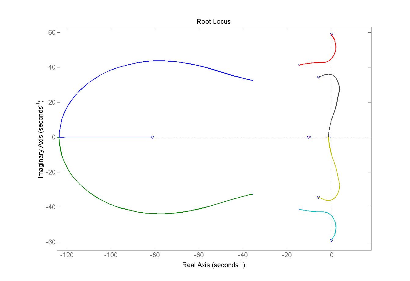
The root locus of T(s)+D(s)𝑇𝑠𝐷𝑠T(s)+D(s) is shown in Figure 4. Clearly, the augmented plant is W-ASPR.
Refer to caption
Figure 4: Root locus of plant with parallel feedforward

The details of implementation in case of CL-SAC are shown in Fig. 5. The parallel feedforward compensator D(s)𝐷𝑠D(s) cannot be implemented parallel to the plant ( shown in dotted line in Fig. 5 ); therefore, the equivalent representation of D(s)𝐷𝑠D(s) is considered through the solid line path.
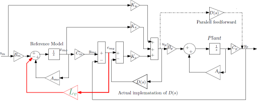
Refer to caption
Figure 5: Details of CL-SAC architecture

The value of σ𝜎\sigma is chosen as 5 . The value of adaptation gains ΓpesubscriptΓ𝑝𝑒\Gamma_{pe} , ΓIesubscriptΓ𝐼𝑒\Gamma_{Ie} , ΓpxsubscriptΓ𝑝𝑥\Gamma_{px} , ΓIxsubscriptΓ𝐼𝑥\Gamma_{Ix} , ΓpusubscriptΓ𝑝𝑢\Gamma_{pu} , ΓIusubscriptΓ𝐼𝑢\Gamma_{Iu} are chosen as 10 in simulation .

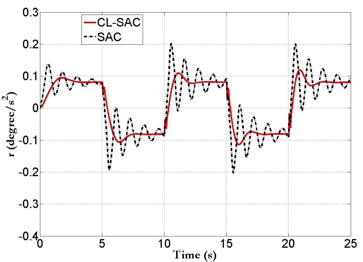
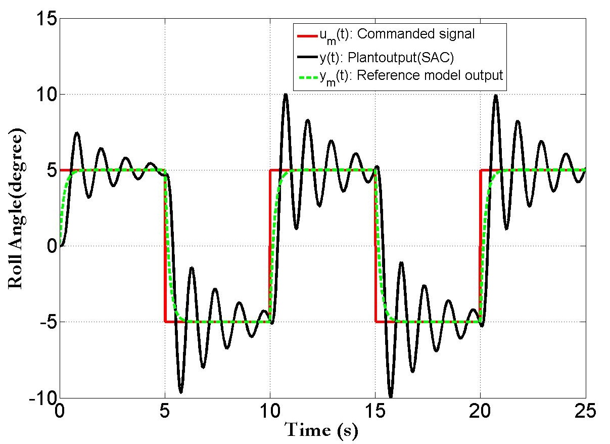
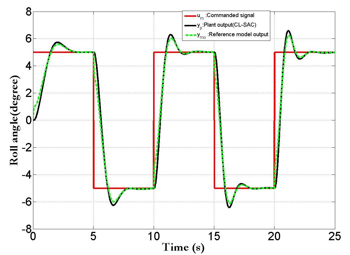
The tracking of the commanded square wave by the SAC and the CL-SAC is plotted in Fig.6 and Fig.7 respectively.
Refer to caption
Figure 6: Reference signal tracking using SAC architecture
Refer to caption
Figure 7: Reference signal tracking using CL-SAC architecture

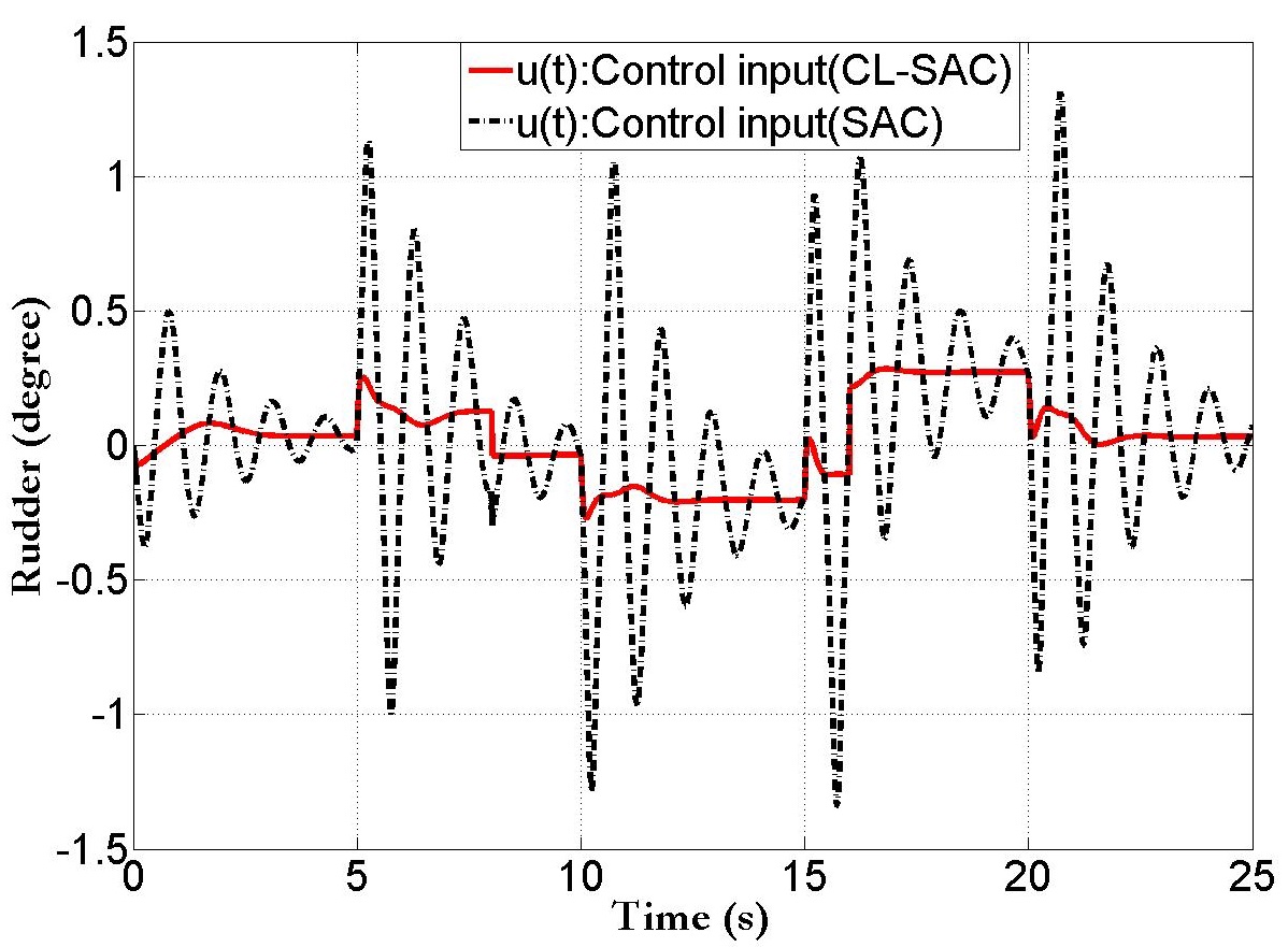
From Fig.6 and Fig.7, it is clear that the tracking performance improves in case of CL-SAC as compared to SAC. Fig. 8 compares the control efforts between both architecture.
Refer to caption
Figure 8: Figure comparing the control input (up)subscript𝑢𝑝(u_{p}) between SAC and CL-SAC

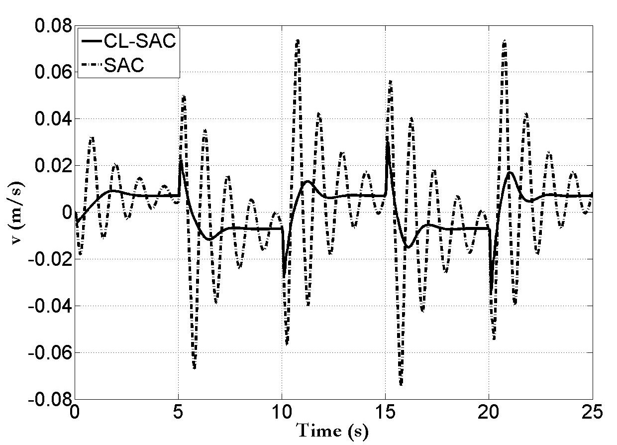
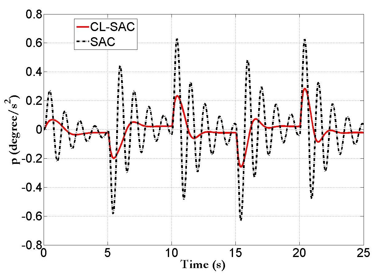
The control efforts in CL-SAC is also less as compared to that of SAC in Fig.8. Clearly, improvement of the transient performance in CL-SAC is obtained without extra control efforts. The variation of other states lateral velocity (v), roll rate (p) and yaw rate (r) are plotted in Fig.9, Fig.10 and Fig.11.
Refer to caption
Figure 9: Figure comparing the lateral velocity between SAC and CL-SAC
Refer to caption
Figure 10: Figure comparing the roll rate between SAC and CL-SAC
Refer to caption
Figure 11: Figure comparing the yaw rate between SAC and CL-SAC

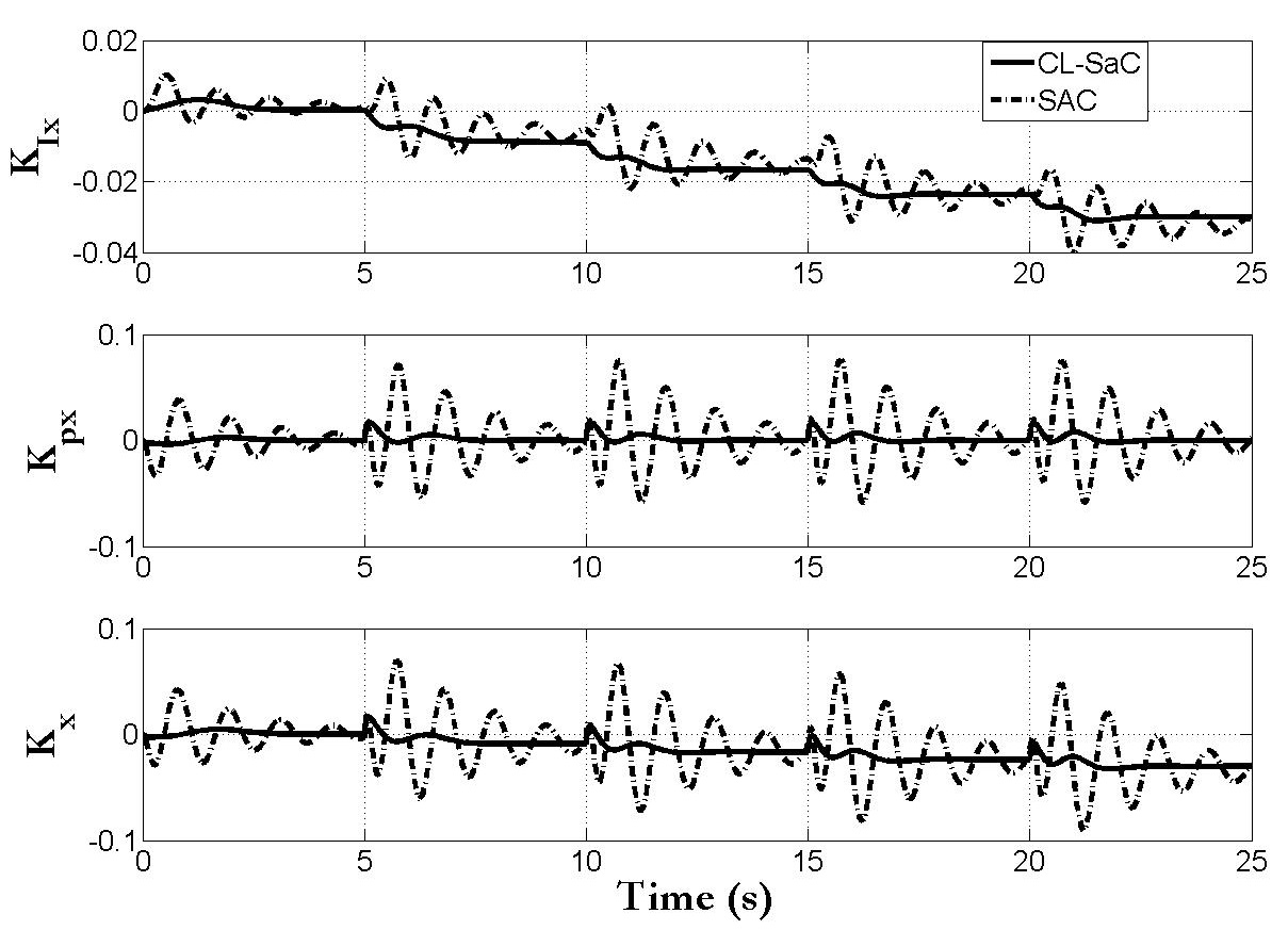
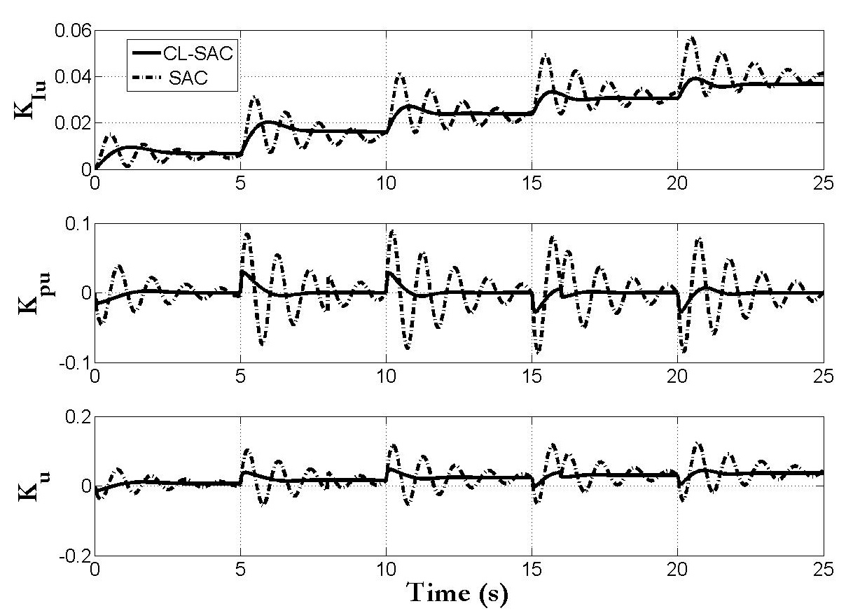
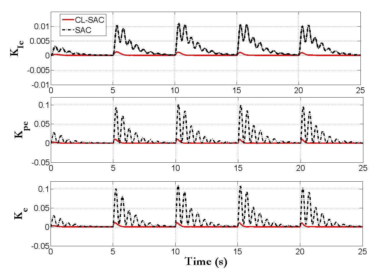
From Fig.9, Fig. 10 and Fig.11; it is evident that the variation of other states in CL-SAC structure is smoother than SAC structure. The control gains Kesubscript𝐾𝑒K_{e}, Kxsubscript𝐾𝑥K_{x}, Kusubscript𝐾𝑢K_{u} are plotted in Fig.12, Fig.13 and Fig.14.
Refer to caption
Figure 12: Figure comparing the value of KIesubscript𝐾𝐼𝑒K_{Ie}, Kpesubscript𝐾𝑝𝑒K_{pe}, Kesubscript𝐾𝑒K_{e} between SAC and CL-SAC
Refer to caption
Figure 13: Figure comparing the value of KIxsubscript𝐾𝐼𝑥K_{Ix}, Kpxsubscript𝐾𝑝𝑥K_{px}, Kxsubscript𝐾𝑥K_{x} between SAC and CL-SAC
Refer to caption
Figure 14: Figure comparing value of KIusubscript𝐾𝐼𝑢K_{Iu}, Kpusubscript𝐾𝑝𝑢K_{pu}, Kusubscript𝐾𝑢K_{u} between SAC and CL-SAC

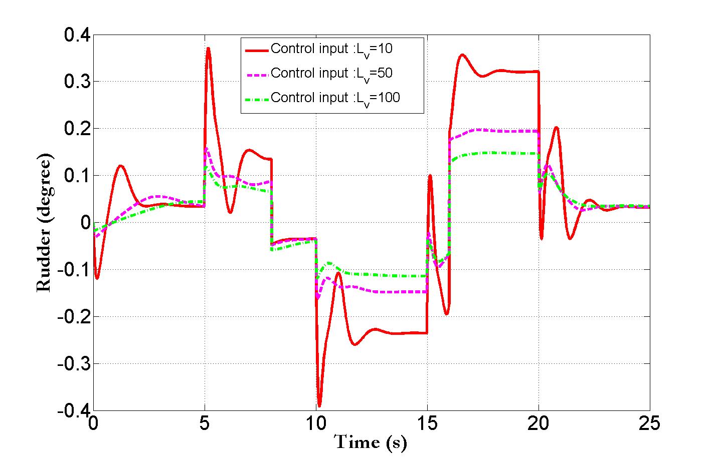
The value of Lvsubscript𝐿𝑣L_{v} needs to be chosen appropriately. The variation in tracking response is investigated with three different values of output error feedback gain; Lvsubscript𝐿𝑣L_{v} =10, 50 and 100. The variation in tracking performance and control input with the variation of (Lvsubscript𝐿𝑣L_{v}) is shown in Fig.15 and Fig.16.

Refer to caption
Figure 15: Figure comparing the tracking response for different value of Lvsubscript𝐿𝑣L_{v}
Refer to caption
Figure 16: Figure comparing control response for different value of Lvsubscript𝐿𝑣L_{v}

Clearly from Fig.15, the error dynamics between the plant output and the close loop reference model output becomes faster with the increase in the value of (Lvsubscript𝐿𝑣L_{v}), however, it causes poor tracking of the output of the open loop reference model; hence poor tracking of original reference command. The lower value of Lvsubscript𝐿𝑣L_{v} will have less effect on error feedback term, where the high value of Lvsubscript𝐿𝑣L_{v} can cause poor tracking of the output of open loop reference model. As output error reduces with a higher value of (Lvsubscript𝐿𝑣L_{v}), the control effort also reduces; which is evident from Fig.16.

5.2 Discussions

From the simulation of lateral model dynamics, it is clear that the roll attitude tracking performance during transient phase is better in the case of CL-SAC as compared to SAC without additional control efforts. So, the output error feedback term in reference model dynamics improves the performance of the system. However, the gain of the output error feedback term needs to be chosen properly as per performance specification and available actuator. The optimum design of Lvsubscript𝐿𝑣L_{v} for CL-SAC structure should be investigated in future studies.

6 Conclusions

In this paper new CL-SAC architecture is proposed after modification of SAC architecture with closed loop reference model based on output feedback. The proposed architecture is based on the intuition that output tracking error feedback in the reference model dynamics will help the plant to follow the reference model. It is shown through mathematical analysis and simulations of lateral model dynamics of Micro Air Vehicle that CL-SAC improves the transient performance without additional control requirement.

Acknowledgements.
The authors would like to thank ARDB and NPMICAV program for partial funding of this work.

References

  • (1) Barkana, I.: Classical and simple adaptive control for nonminimum phase autopilot design. Journal of Guidance, Control, and Dynamics 28(4), 631–638 (2005)
  • (2) Barkana, I.: Simple adaptive control–a stable direct model reference adaptive control methodology–brief survey. International Journal of Adaptive Control and Signal Processing 28(7-8), 567–603 (2014)
  • (3) Barkana, I.: Adaptive control? but is so simple! a tribute to the efficiency, simplicity and beauty of adaptive control. Journal of Intelligent & Robotic Systems 83(1), 3–34 (2016)
  • (4) Barkana, I.: Robustness and perfect tracking in simple adaptive control. International Journal of Adaptive Control and Signal Processing 30(8-10), 1118–1151 (2016)
  • (5) Broussard, J., O’Brien, M.: Feedforward control to track the output of a forced model. IEEE Transactions on Automatic control 25(4), 851–853 (1980)
  • (6) Gibson, T., Annaswamy, A., Lavretsky, E.: Closed–loop reference model adaptive control, part i: Transient performance,”. In: American Control Conference, pp. 3376–3383 (2013)
  • (7) Gibson, T.E., Annaswamy, A.M., Lavretsky, E.: On adaptive control with closed-loop reference models: transients, oscillations, and peaking. IEEE Access 1, 703–717 (2013)
  • (8) Harikumar, K., Dhall, S., Bhat, M.S.: Nonlinear modeling and control of coupled dynamics of a fixed wing micro air vehicle. In: Control Conference (ICC), 2016 Indian, pp. 318–323. IEEE (2016)
  • (9) Ioannou, P.A., Sun, J.: Robust adaptive control. Courier Corporation (2012)
  • (10) Jana, S., Bhat, M.S.: Closed loop reference model simple adaptive control for micro air vehicle. In: Euro GNC, 4th CEAS Specialist Conference on Guidance, Navigation and Control (2017)
  • (11) Jeong, G.J., Kim, I.H., Son, Y.I.: Design of an adaptive output feedback controller for a dc/dc boost converter subject to load variation. International Journal of Innovative Computing, Information and Control 7(2), 791–803 (2011)
  • (12) Kaufman, H., Barkana, I., Sobel, K.: Direct adaptive control algorithms: theory and applications. Springer Science & Business Media (2012)
  • (13) Lavretsky, E., Wise, K.: Robust and adaptive control: With aerospace applications, ser. Advanced textbooks in control and signal processing. London and New York: Springer (2013)
  • (14) Maganti, G.B., Singh, S.N.: Simplified adaptive control of an orbiting flexible spacecraft. Acta Astronautica 61(7), 575–589 (2007)
  • (15) Narendra, K.S., Annaswamy, A.M.: Stable adaptive systems. Courier Corporation (2012)
  • (16) Rusnak, I., Barkana, I.: The duality of parallel feedforward and negative feedback. In: Electrical & Electronics Engineers in Israel (IEEEI), 2012 IEEE 27th Convention of, pp. 1–4. IEEE (2012)
  • (17) Slotine, J.J.E., Li, W., et al.: Applied nonlinear control, vol. 199. Prentice hall Englewood Cliffs, NJ (1991)
  • (18) Stepanyan, V., Krishnakumar, K.: Mrac revisited: guaranteed performance with reference model modification. In: American Control Conference (ACC), 2010, pp. 93–98. IEEE (2010)
  • (19) Stepanyan, V., Krishnakumar, K.S.: Output feedback m-mrac. In: AIAA Guidance, Navigation, and Control (GNC) Conference, p. 4612 (2013)
  • (20) Tomashevich, S.I., Fradkov, A.L., Andrievsky, B., Belyavskyi, A.O., Amelin, K.: Simple adaptive control of quadrotor attitude. algorithms and experimental results. In: Control and Automation (MED), 2017 25th Mediterranean Conference on, pp. 933–938. IEEE (2017)
  • (21) Ulrich, S., Sasiadek, J.Z., Barkana, I.: Nonlinear adaptive output feedback control of flexible-joint space manipulators with joint stiffness uncertainties. Journal of Guidance, Control, and Dynamics 37(6), 1961–1975 (2014)
  • (22) Wiese, D.P., Annaswamy, A.M., Muse, J.A., Bolender, M.A., Lavretsky, E.: Adaptive output feedback based on closed-loop reference models for hypersonic vehicles. Journal of Guidance, Control, and Dynamics 38(12), 2429–2440 (2015)
  • (23) Yasuda, K., Hirai, K.: Upper and lower bounds on the solution of the algebraic riccati equation. IEEE Transactions on Automatic Control 24(3), 483–487 (1979)