Abstract
Let ( 𝔻 2 , ℱ , { 0 } ) superscript 𝔻 2 ℱ 0 (\mathbb{D}^{2},\mathscr{F},\{0\}) 𝔻 2 superscript 𝔻 2 \mathbb{D}^{2}
z ∂ ∂ z + λ w ∂ ∂ w , 𝑧 𝑧 𝜆 𝑤 𝑤 z\,\frac{\partial}{\partial z}+\lambda\,w\,\frac{\partial}{\partial w},
where λ ∈ ℂ ∗ 𝜆 superscript ℂ \lambda\in\mathbb{C}^{*} 0 0 T 𝑇 T ℱ ℱ \mathscr{F} ( z = 0 ) 𝑧 0 (z=0) ( w = 0 ) 𝑤 0 (w=0) T ~ ~ 𝑇 \tilde{T} 0 0 d d c 𝑑 superscript 𝑑 𝑐 dd^{c} T 𝑇 T 0 0 λ ∉ ℝ 𝜆 ℝ \lambda\notin\mathbb{R} 0 0 0 0 λ ∈ ℝ ∗ 𝜆 superscript ℝ \lambda\in\mathbb{R}^{*} 0 0
1) is strictly positive if λ > 0 𝜆 0 \lambda>0
2) vanishes if λ ∈ ℚ < 0 𝜆 subscript ℚ absent 0 \lambda\in\mathbb{Q}_{<0}
3) vanishes if λ < 0 𝜆 0 \lambda<0 T 𝑇 T
1 Introduction
The dynamical properties of holomorphic foliations have drawn great attention recently [40 ] . Let us see one of the recent interesting results.
Theorem 1.1 (Dinh-Nguyên-Sibony [20 ] ).
Let ℱ ℱ \mathscr{F} ( X , ω ) 𝑋 𝜔 (X,\omega) ℱ ℱ \mathscr{F} d d c 𝑑 superscript 𝑑 𝑐 dd^{c} T 𝑇 T 1 1 1 ℱ ℱ \mathscr{F}
The first version was stated for X = ℙ 2 𝑋 superscript ℙ 2 X=\mathbb{P}^{2} [28 ] . Later Dinh-Sibony proved unique ergodicity for foliations in ℙ 2 superscript ℙ 2 \mathbb{P}^{2} [23 ] . So one may expect to describe recurrence properties of leaves by studying the density distribution of directed harmonic currents. One has the following the result about leaves.
Theorem 1.2 (Fornæss-Sibony [28 ] ).
Let ( X , ℱ , E ) 𝑋 ℱ 𝐸 (X,\mathscr{F},E) X 𝑋 X E 𝐸 E
1.
there is no invariant analytic curve;
2.
all the singularities are hyperbolic;
3.
there is no non-constant holomorphic map ℂ → X → ℂ 𝑋 \mathbb{C}\rightarrow X such that out of E 𝐸 E the image of ℂ ℂ \mathbb{C} is locally contained in a leaf.
Then every harmonic current T 𝑇 T ℱ ℱ \mathscr{F}
A practical way to measure the density of harmonic currents is to use the notion of Lelong number introduced by Skoda [49 ] . Indeed Theorem 1.2 T 𝑇 T E 𝐸 E
Theorem 1.3 (Nguyên [34 ] ).
Let ( 𝔻 2 , ℱ , { 0 } ) superscript 𝔻 2 ℱ 0 (\mathbb{D}^{2},\mathscr{F},\{0\}) 𝔻 2 superscript 𝔻 2 \mathbb{D}^{2} Z ( z , w ) = z ∂ ∂ z + λ w ∂ ∂ w , 𝑍 𝑧 𝑤 𝑧 𝑧 𝜆 𝑤 𝑤 Z(z,w)=z\,\frac{\partial}{\partial z}+\lambda\,w\,\frac{\partial}{\partial w}, λ ∈ ℂ \ ℝ 𝜆 \ ℂ ℝ \lambda\in\mathbb{C}\backslash\mathbb{R} 0 0 T 𝑇 T ℱ ℱ \mathscr{F} ( z = 0 ) 𝑧 0 (z=0) ( w = 0 ) 𝑤 0 (w=0) T 𝑇 T 0 0
Nguyên proved that the Lelong number of any directed harmonic current which gives no mass to invariant hyperplanes, vanishes near weakly hyperbolic singularities in ℂ n superscript ℂ 𝑛 \mathbb{C}^{n} [40 ] . This result is optimal, see [25 ] . The mass-distribution problem would be completed once the behaviour of harmonic currents near non-hyperbolic and near degenerate singularities would be understood.
The present paper answers (partly) the problem in the non-hyperbolic linearizable singularity case.
Theorem 1.4 .
Let ( 𝔻 2 , ℱ , { 0 } ) superscript 𝔻 2 ℱ 0 (\mathbb{D}^{2},\mathscr{F},\{0\}) 𝔻 2 superscript 𝔻 2 \mathbb{D}^{2} Z ( z , w ) = z ∂ ∂ z + λ w ∂ ∂ w 𝑍 𝑧 𝑤 𝑧 𝑧 𝜆 𝑤 𝑤 Z(z,w)=z\,\frac{\partial}{\partial z}+\lambda\,w\,\frac{\partial}{\partial w} λ ∈ ℝ ∗ 𝜆 superscript ℝ \lambda\in\mathbb{R}^{*} ℱ ℱ \mathscr{F} ℱ ℱ \mathscr{F} ( z = 0 ) 𝑧 0 (z=0) ( w = 0 ) 𝑤 0 (w=0) T 𝑇 T 0 0
•
is strictly positive if λ > 0 𝜆 0 \lambda>0 ,
•
vanishes if λ ∈ ℚ < 0 𝜆 subscript ℚ absent 0 \lambda\in\mathbb{Q}_{<0} .
For the concerned foliation ( 𝔻 2 , ℱ , { 0 } ) superscript 𝔻 2 ℱ 0 (\mathbb{D}^{2},\mathscr{F},\{0\}) P α subscript 𝑃 𝛼 P_{\alpha} α ∈ ℂ ∗ 𝛼 superscript ℂ \alpha\in\mathbb{C}^{*} ( z , w ) = ( e − v + i u , α e − λ v + i λ u ) 𝑧 𝑤 superscript 𝑒 𝑣 𝑖 𝑢 𝛼 superscript 𝑒 𝜆 𝑣 𝑖 𝜆 𝑢 (z,w)=(e^{-v+iu},\alpha\,e^{-\lambda v+i\lambda u}) monodromy group around the singularity is generated by ( z , w ) ↦ ( z , e 2 π i λ w ) maps-to 𝑧 𝑤 𝑧 superscript 𝑒 2 𝜋 𝑖 𝜆 𝑤 (z,w)\mapsto(z,e^{2\pi i\lambda}w) λ ∈ ℚ ∗ 𝜆 superscript ℚ \lambda\in\mathbb{Q}^{*} λ ∉ ℚ 𝜆 ℚ \lambda\notin\mathbb{Q}
It is now ready to introduce the notion of periodic current , an essential tool of this paper. A directed harmonic current T 𝑇 T periodic if it is invariant under some cofinite subgroup of the monodromy group, i.e. under the action of ( z , w ) ↦ ( z , e 2 k π i λ w ) maps-to 𝑧 𝑤 𝑧 superscript 𝑒 2 𝑘 𝜋 𝑖 𝜆 𝑤 (z,w)\mapsto(z,e^{2k\pi i\lambda}w) k ∈ ℤ > 0 𝑘 subscript ℤ absent 0 k\in\mathbb{Z}_{>0} λ ∈ ℚ ∗ 𝜆 superscript ℚ \lambda\in\mathbb{Q}^{*} λ ∉ ℚ ∗ 𝜆 superscript ℚ \lambda\notin\mathbb{Q}^{*}
Theorem 1.5 .
Using the same notation as above, the Lelong number of T 𝑇 T λ < 0 𝜆 0 \lambda<0 λ ∈ ℚ < 0 𝜆 subscript ℚ absent 0 \lambda\in\mathbb{Q}_{<0}
It remains open to determine the possible Lelong number values of non-periodic T 𝑇 T λ < 0 𝜆 0 \lambda<0
2 Background
To start with, recall the definition of singular holomorphic foliation on a complex surface M 𝑀 M
Definition 2.1 .
Let E ⊂ M 𝐸 𝑀 E\subset M M \ E ¯ = M ¯ \ 𝑀 𝐸 𝑀 \overline{M\backslash E}=M singular holomorphic foliation ( M , E , ℱ ) 𝑀 𝐸 ℱ (M,E,\mathscr{F}) atlas { ( 𝕌 i , Φ i ) } i ∈ I subscript subscript 𝕌 𝑖 subscript Φ 𝑖 𝑖 𝐼 \{(\mathbb{U}_{i},\Phi_{i})\}_{i\in I} M \ E \ 𝑀 𝐸 M\backslash E
(1)
For each i ∈ I 𝑖 𝐼 i\in I Φ i : 𝕌 i → 𝔹 i × 𝕋 i : subscript Φ 𝑖 → subscript 𝕌 𝑖 subscript 𝔹 𝑖 subscript 𝕋 𝑖 \Phi_{i}:\mathbb{U}_{i}\rightarrow\mathbb{B}_{i}\times\mathbb{T}_{i} 𝔹 i subscript 𝔹 𝑖 \mathbb{B}_{i} 𝕋 i subscript 𝕋 𝑖 \mathbb{T}_{i} ℂ ℂ \mathbb{C}
(2)
For each pair ( 𝕌 i , Φ i ) subscript 𝕌 𝑖 subscript Φ 𝑖 (\mathbb{U}_{i},\Phi_{i}) ( 𝕌 j , Φ j ) subscript 𝕌 𝑗 subscript Φ 𝑗 (\mathbb{U}_{j},\Phi_{j}) 𝕌 i ∩ 𝕌 j ≠ ∅ subscript 𝕌 𝑖 subscript 𝕌 𝑗 \mathbb{U}_{i}\cap\mathbb{U}_{j}\neq\emptyset
Φ i j := Φ i ∘ Φ j − 1 : Φ j ( 𝕌 i ∩ 𝕌 j ) → Φ i ( 𝕌 i ∩ 𝕌 j ) : assign subscript Φ 𝑖 𝑗 subscript Φ 𝑖 superscript subscript Φ 𝑗 1 → subscript Φ 𝑗 subscript 𝕌 𝑖 subscript 𝕌 𝑗 subscript Φ 𝑖 subscript 𝕌 𝑖 subscript 𝕌 𝑗 \Phi_{ij}:=\Phi_{i}\circ\Phi_{j}^{-1}:\Phi_{j}(\mathbb{U}_{i}\cap\mathbb{U}_{j})\rightarrow\Phi_{i}(\mathbb{U}_{i}\cap\mathbb{U}_{j})
has the form
Φ i j ( b , t ) = ( Ω ( b , t ) , Λ ( t ) ) , subscript Φ 𝑖 𝑗 𝑏 𝑡 Ω 𝑏 𝑡 Λ 𝑡 \Phi_{ij}(b,t)=\big{(}\Omega(b,t),\Lambda(t)\big{)},
where ( b , t ) 𝑏 𝑡 (b,t) 𝔹 j × 𝕋 j subscript 𝔹 𝑗 subscript 𝕋 𝑗 \mathbb{B}_{j}\times\mathbb{T}_{j} Ω Ω \Omega Λ Λ \Lambda Λ Λ \Lambda b 𝑏 b
Each open set 𝕌 i subscript 𝕌 𝑖 \mathbb{U}_{i} flow box . For each c ∈ 𝕋 i 𝑐 subscript 𝕋 𝑖 c\in\mathbb{T}_{i} Φ i − 1 { t = c } superscript subscript Φ 𝑖 1 𝑡 𝑐 \Phi_{i}^{-1}\{t=c\} 𝕌 i subscript 𝕌 𝑖 \mathbb{U}_{i} plaque . The property (2) above insures that in the intersection of two flow boxes, plaques are mapped to plaques.
A leaf L 𝐿 L M 𝑀 M L 𝐿 L transversal is a Riemann surface immersed in M 𝑀 M M 𝑀 M
The local theory of singular holomorphic foliations is closely related to holomorphic vector fields. One recalls some basic concepts in ℂ 2 superscript ℂ 2 \mathbb{C}^{2} [40 ] , [14 ] ).
Definition 2.2 .
Let Z = P ( z , w ) ∂ ∂ z + Q ( z , w ) ∂ ∂ w 𝑍 𝑃 𝑧 𝑤 𝑧 𝑄 𝑧 𝑤 𝑤 Z=P(z,w)\frac{\partial}{\partial z}+Q(z,w)\frac{\partial}{\partial w} 𝕌 𝕌 \mathbb{U} ( 0 , 0 ) ∈ ℂ 2 0 0 superscript ℂ 2 (0,0)\in\mathbb{C}^{2} Z 𝑍 Z
(1)
singular at ( 0 , 0 ) 0 0 (0,0) P ( 0 , 0 ) = Q ( 0 , 0 ) = 0 𝑃 0 0 𝑄 0 0 0 P(0,0)=Q(0,0)=0
(2)
linear if it can be written as
Z = λ 1 z ∂ ∂ z + λ 2 w ∂ ∂ w 𝑍 subscript 𝜆 1 𝑧 𝑧 subscript 𝜆 2 𝑤 𝑤 Z=\lambda_{1}z\frac{\partial}{\partial z}+\lambda_{2}w\frac{\partial}{\partial w}
where λ 1 subscript 𝜆 1 \lambda_{1} λ 2 ∈ ℂ subscript 𝜆 2 ℂ \lambda_{2}\in\mathbb{C}
(3)
linearizable if it is linear after a biholomorphic change of coordinates.
Suppose the holomorphic vector field Z = P ∂ ∂ z + Q ∂ ∂ w 𝑍 𝑃 𝑧 𝑄 𝑤 Z=P\frac{\partial}{\partial z}+Q\frac{\partial}{\partial w} λ 1 subscript 𝜆 1 \lambda_{1} λ 2 subscript 𝜆 2 \lambda_{2} ( P z P w Q z Q w ) subscript 𝑃 𝑧 subscript 𝑃 𝑤 subscript 𝑄 𝑧 subscript 𝑄 𝑤 \textstyle\left(\!\begin{array}[]{cc}P_{z}&P_{w}\\
Q_{z}&Q_{w}\end{array}\!\right)
Definition 2.3 .
The singularity is non-degenerate if both λ 1 subscript 𝜆 1 \lambda_{1} λ 2 subscript 𝜆 2 \lambda_{2}
In this article, all singularities are assumed to be non-degenerate. Then the foliation defined by integral curves of Z 𝑍 Z 0 0 [14 ] . Seidenberg’s reduction theorem [46 ] shows that degenerate singularites can be resolved into non-degenerate ones after finitely many blow-ups.
Definition 2.4 .
A singularity of Z 𝑍 Z hyperbolic if the quotient λ := λ 1 λ 2 ∈ ℂ ∗ \ ℝ assign 𝜆 subscript 𝜆 1 subscript 𝜆 2 \ superscript ℂ ℝ \lambda:=\frac{\lambda_{1}}{\lambda_{2}}\in\mathbb{C}^{*}\backslash\mathbb{R} non-hyperbolic if λ ∈ ℝ ∗ 𝜆 superscript ℝ \lambda\in\mathbb{R}^{*} Poincaré domain if λ ∉ ℝ ⩽ 0 𝜆 subscript ℝ absent 0 \lambda\notin\mathbb{R}_{\leqslant 0} Siegel domain if λ ∈ ℝ < 0 𝜆 subscript ℝ absent 0 \lambda\in\mathbb{R}_{<0}
One can verify that the quotient is unchanged by multiplication of Z 𝑍 Z
One could consider λ − 1 = λ 2 λ 1 superscript 𝜆 1 subscript 𝜆 2 subscript 𝜆 1 \lambda^{-1}=\frac{\lambda_{2}}{\lambda_{1}} λ 𝜆 \lambda λ ∉ ℝ 𝜆 ℝ \lambda\notin\mathbb{R} λ − 1 ∉ ℝ superscript 𝜆 1 ℝ \lambda^{-1}\notin\mathbb{R} λ 𝜆 \lambda eigenvalue of Z 𝑍 Z λ ↔ λ − 1 ↔ 𝜆 superscript 𝜆 1 \lambda\leftrightarrow\lambda^{-1} { λ , λ − 1 } 𝜆 superscript 𝜆 1 \{\lambda,\lambda^{-1}\}
Consider a holomorphic foliation ( M , E , ℱ ) 𝑀 𝐸 ℱ (M,E,\mathscr{F}) E 𝐸 E λ 1 m 1 + λ 2 m 2 − λ j subscript 𝜆 1 subscript 𝑚 1 subscript 𝜆 2 subscript 𝑚 2 subscript 𝜆 𝑗 \lambda_{1}\,m_{1}+\lambda_{2}\,m_{2}-\lambda_{j} j = 1 , 2 𝑗 1 2
j=1,2 m 1 subscript 𝑚 1 m_{1} m 2 ∈ ℤ ⩾ 1 subscript 𝑚 2 subscript ℤ absent 1 m_{2}\in\mathbb{Z}_{\geqslant 1}
The resonances of ( λ 1 , λ 2 ) ∈ ℂ 2 subscript 𝜆 1 subscript 𝜆 2 superscript ℂ 2 (\lambda_{1},\lambda_{2})\in\mathbb{C}^{2}
ℛ := { ( m 1 , m 2 , j ) ∈ ℤ 3 | m 1 , m 2 ∈ ℤ ⩾ 1 , λ 1 m 1 + λ 2 m 2 − λ j = 0 } . assign ℛ conditional-set subscript 𝑚 1 subscript 𝑚 2 𝑗 superscript ℤ 3 formulae-sequence subscript 𝑚 1 subscript 𝑚 2
subscript ℤ absent 1 subscript 𝜆 1 subscript 𝑚 1 subscript 𝜆 2 subscript 𝑚 2 subscript 𝜆 𝑗 0 \mathcal{R}:=\{(m_{1},m_{2},j)\in\mathbb{Z}^{3}~{}|~{}m_{1},\,m_{2}\in\mathbb{Z}_{\geqslant 1},~{}\lambda_{1}\,m_{1}+\lambda_{2}\,m_{2}-\lambda_{j}=0\}.
Notice that the set { λ 1 m 1 + λ 2 m 2 − λ j | m 1 , m 2 ∈ ℤ ⩾ 1 } conditional-set subscript 𝜆 1 subscript 𝑚 1 subscript 𝜆 2 subscript 𝑚 2 subscript 𝜆 𝑗 subscript 𝑚 1 subscript 𝑚 2
subscript ℤ absent 1 \{\lambda_{1}\,m_{1}+\lambda_{2}\,m_{2}-\lambda_{j}~{}|~{}m_{1},m_{2}\in\mathbb{Z}_{\geqslant 1}\}
We are now ready to state some linearization results in ℂ 2 superscript ℂ 2 \mathbb{C}^{2}
Theorem 2.5 (Poincaré [5 ] ).
A singular holomorphic vector field with a non-resonant linear part, i.e. ℛ ℛ \mathcal{R} λ 𝜆 \lambda
That is to say, a singularity is linearizable if λ ∉ ℝ ⩽ 0 ∪ ℚ 𝜆 subscript ℝ absent 0 ℚ \lambda\notin\mathbb{R}_{\leqslant 0}\cup\mathbb{Q} λ 𝜆 \lambda Brjuno condition .
Theorem 2.6 (Brjuno [5 , 11 ] ).
A singular holomorphic vector field with a non-resonant linear part is holomorphically linearizable if its eigenvalue λ ∈ ℝ 𝜆 ℝ \lambda\in\mathbb{R}
∑ n ⩾ 1 log q n + 1 q n < ∞ , subscript 𝑛 1 subscript 𝑞 𝑛 1 subscript 𝑞 𝑛 \sum_{n\geqslant 1}\frac{\log q_{n+1}}{q_{n}}<\infty,
where p n / q n subscript 𝑝 𝑛 subscript 𝑞 𝑛 p_{n}/q_{n} n 𝑡ℎ superscript 𝑛 𝑡ℎ n^{\sl th} λ 𝜆 \lambda
In this article, all singularities are assumed to be linearizable. Let ( 𝔻 2 , ℱ , { 0 } ) superscript 𝔻 2 ℱ 0 (\mathbb{D}^{2},\mathscr{F},\{0\}) 𝔻 2 superscript 𝔻 2 \mathbb{D}^{2} Z = z ∂ ∂ z + λ w ∂ ∂ w 𝑍 𝑧 𝑧 𝜆 𝑤 𝑤 Z=z\frac{\partial}{\partial z}+\lambda w\frac{\partial}{\partial w} λ ∈ ℝ ∗ 𝜆 superscript ℝ \lambda\in\mathbb{R}^{*} 0 < | λ | ⩽ 1 0 𝜆 1 0<|\lambda|\leqslant 1 z 𝑧 z w 𝑤 w { z = 0 } 𝑧 0 \{z=0\} { w = 0 } 𝑤 0 \{w=0\}
L α := { ( z , w ) = ψ α ( ζ ) := ( e i ζ , α e i λ ζ ) = ( e − v + i u , α e − λ v + i λ u ) } ( α ≠ 0 ) , assign subscript 𝐿 𝛼 𝑧 𝑤 subscript 𝜓 𝛼 𝜁 assign superscript 𝑒 𝑖 𝜁 𝛼 superscript 𝑒 𝑖 𝜆 𝜁 superscript 𝑒 𝑣 𝑖 𝑢 𝛼 superscript 𝑒 𝜆 𝑣 𝑖 𝜆 𝑢 𝛼 0
L_{\alpha}:=\{(z,w)=\psi_{\alpha}(\zeta):=(e^{i\,\zeta},\alpha\,e^{i\,\lambda\,\zeta})=(e^{-v+i\,u},\alpha\,e^{-\lambda\,v+i\,\lambda\,u})\}\quad{\scriptstyle{(\alpha\neq 0)}},
where ζ = u + i v ∈ ℂ 𝜁 𝑢 𝑖 𝑣 ℂ \zeta=u+iv\in\mathbb{C}
Ψ : ℂ × ℂ ∗ : Ψ ℂ superscript ℂ \displaystyle\Psi:\mathbb{C}\times\mathbb{C}^{*} ⟶ ℂ 2 , ⟶ absent superscript ℂ 2 \displaystyle\longrightarrow\mathbb{C}^{2},
( ζ , α ) 𝜁 𝛼 \displaystyle(\zeta,\alpha) ⟼ ( e i ζ , α e i λ ζ ) , ⟼ absent superscript 𝑒 𝑖 𝜁 𝛼 superscript 𝑒 𝑖 𝜆 𝜁 \displaystyle\longmapsto(e^{i\,\zeta},\alpha\,e^{i\,\lambda\,\zeta}),
is locally biholomorphic. Here α 𝛼 \alpha ζ 𝜁 \zeta Ψ ( ζ + 2 π , α ) = Ψ ( ζ , α e 2 π i λ ) Ψ 𝜁 2 𝜋 𝛼 Ψ 𝜁 𝛼 superscript 𝑒 2 𝜋 𝑖 𝜆 \Psi(\zeta+2\pi,\alpha)=\Psi(\zeta,\alpha\,e^{2\pi i\lambda})
Two numbers α 𝛼 \alpha β ∈ ℂ ∗ 𝛽 superscript ℂ \beta\in\mathbb{C}^{*} equivalent α ∼ β similar-to 𝛼 𝛽 \alpha\sim\beta β = e 2 k π i λ α 𝛽 superscript 𝑒 2 𝑘 𝜋 𝑖 𝜆 𝛼 \beta=e^{2k\pi i\lambda}\alpha k ∈ ℤ 𝑘 ℤ k\in\mathbb{Z}
•
α ∼ β similar-to 𝛼 𝛽 \alpha\sim\beta
•
L α = L β subscript 𝐿 𝛼 subscript 𝐿 𝛽 L_{\alpha}=L_{\beta}
•
ψ α = ψ β ∘ ( translation of 2 k π ) subscript 𝜓 𝛼 subscript 𝜓 𝛽 translation of 2 𝑘 𝜋 \psi_{\alpha}=\psi_{\beta}\circ(\text{translation of }2k\pi) k ∈ ℤ 𝑘 ℤ k\in\mathbb{Z}
Let 𝒞 ℱ subscript 𝒞 ℱ \mathscr{C}_{\mathscr{F}} 𝒞 ℱ 1 , 1 superscript subscript 𝒞 ℱ 1 1
\mathscr{C}_{\mathscr{F}}^{1,1} ( resp. forms of bidegree (1,1)) defined on leaves of the foliation which are compactly supported on M \ E \ 𝑀 𝐸 M\backslash E ι ∈ 𝒞 ℱ 1 , 1 𝜄 superscript subscript 𝒞 ℱ 1 1
\iota\in\mathscr{C}_{\mathscr{F}}^{1,1} positive if its restriction to every plaque is a positive (1,1)-form.
A directed harmonic current T 𝑇 T ℱ ℱ \mathscr{F} is a continuous linear form on 𝒞 ℱ 1 , 1 superscript subscript 𝒞 ℱ 1 1
\mathscr{C}_{\mathscr{F}}^{1,1}
1.
i ∂ ∂ ¯ T = 0 𝑖 ¯ 𝑇 0 i\partial\bar{\partial}T=0 T ( i ∂ ∂ ¯ f ) = 0 𝑇 𝑖 ¯ 𝑓 0 T(i\partial\bar{\partial}f)=0 f ∈ 𝒞 ℱ 𝑓 subscript 𝒞 ℱ f\in\mathscr{C}_{\mathscr{F}} i ∂ ∂ f ¯ 𝑖 ¯ 𝑓 i\partial\bar{\partial f} ∂ ∂ ¯ ¯ \partial\bar{\partial}
2.
T 𝑇 T T ( ι ) ⩾ 0 𝑇 𝜄 0 T(\iota)\geqslant 0 ι ∈ 𝒞 ℱ 1 , 1 𝜄 superscript subscript 𝒞 ℱ 1 1
\iota\in\mathscr{C}_{\mathscr{F}}^{1,1}
According to [8 ] , a directed harmonic current T 𝑇 T 𝕌 ≅ 𝔹 × 𝕋 𝕌 𝔹 𝕋 \mathbb{U}\cong\mathbb{B}\times\mathbb{T}
T = ∫ α ∈ 𝕋 h α [ P α ] 𝑑 μ ( α ) . 𝑇 subscript 𝛼 𝕋 subscript ℎ 𝛼 delimited-[] subscript 𝑃 𝛼 differential-d 𝜇 𝛼 T=\int_{\alpha\in\mathbb{T}}h_{\alpha}[P_{\alpha}]d\mu(\alpha). (1)
The h α subscript ℎ 𝛼 h_{\alpha} P α subscript 𝑃 𝛼 P_{\alpha} μ 𝜇 \mu 𝕋 𝕋 \mathbb{T} h α = 0 subscript ℎ 𝛼 0 h_{\alpha}=0 P α subscript 𝑃 𝛼 P_{\alpha} h α ≡ 0 subscript ℎ 𝛼 0 h_{\alpha}\equiv 0 α ∈ 𝕋 𝛼 𝕋 \alpha\in\mathbb{T} h α subscript ℎ 𝛼 h_{\alpha} 1 1 1 d μ ( α ) = 0 𝑑 𝜇 𝛼 0 d\mu(\alpha)=0 T 𝑇 T h α > 0 subscript ℎ 𝛼 0 h_{\alpha}>0 α ∈ 𝕋 𝛼 𝕋 \alpha\in\mathbb{T}
Such an expression is not unique since T = ∫ α ∈ 𝕋 ( h α g ( α ) ) [ P α ] ( 1 g ( α ) d μ ( α ) ) 𝑇 subscript 𝛼 𝕋 subscript ℎ 𝛼 𝑔 𝛼 delimited-[] subscript 𝑃 𝛼 1 𝑔 𝛼 𝑑 𝜇 𝛼 T=\int_{\alpha\in\mathbb{T}}\big{(}h_{\alpha}\,g(\alpha)\big{)}[P_{\alpha}]\big{(}\frac{1}{g(\alpha)}\,d\mu(\alpha)\big{)} g : 𝕋 → ℝ > 0 : 𝑔 → 𝕋 subscript ℝ absent 0 g:\mathbb{T}\rightarrow\mathbb{R}_{>0} normalization , which means that for each α ∈ 𝕋 𝛼 𝕋 \alpha\in\mathbb{T} h α ( z 0 , w 0 ) = 1 subscript ℎ 𝛼 subscript 𝑧 0 subscript 𝑤 0 1 h_{\alpha}(z_{0},w_{0})=1 ( z 0 , w 0 ) ∈ P α subscript 𝑧 0 subscript 𝑤 0 subscript 𝑃 𝛼 (z_{0},w_{0})\in P_{\alpha}
Each harmonic function h α subscript ℎ 𝛼 h_{\alpha} V α subscript 𝑉 𝛼 V_{\alpha} Ψ Ψ \Psi
H α ( u , v ) := h α ( e − v + i u , α e − λ v + i λ u ) . assign subscript 𝐻 𝛼 𝑢 𝑣 subscript ℎ 𝛼 superscript 𝑒 𝑣 𝑖 𝑢 𝛼 superscript 𝑒 𝜆 𝑣 𝑖 𝜆 𝑢 H_{\alpha}(u,v):=h_{\alpha}\big{(}e^{-v+iu},\alpha\,e^{-\lambda v+i\lambda u}\big{)}.
The domain of definition for u 𝑢 u v 𝑣 v
In Section 1 periodic current was introduced. Here is an equivalent characterization.
Proposition 2.7 .
A directed harmonic current T 𝑇 T periodic if and only if there exists some k ∈ ℤ > 0 𝑘 subscript ℤ absent 0 k\in\mathbb{Z}_{>0} H α ( u + 2 k π , v ) = H α ( u , v ) subscript 𝐻 𝛼 𝑢 2 𝑘 𝜋 𝑣 subscript 𝐻 𝛼 𝑢 𝑣 H_{\alpha}(u+2k\pi,v)=H_{\alpha}(u,v) u , v 𝑢 𝑣
u,v μ 𝜇 \mu α 𝛼 \alpha
Proof.
By definition T 𝑇 T ( z , w ) ↦ ( z , e 2 k π i λ w ) maps-to 𝑧 𝑤 𝑧 superscript 𝑒 2 𝑘 𝜋 𝑖 𝜆 𝑤 (z,w)\mapsto(z,e^{2k\pi i\lambda}w) k ∈ ℤ > 0 𝑘 subscript ℤ absent 0 k\in\mathbb{Z}_{>0} H α ( u + 2 k π , v ) = H α ( u , v ) subscript 𝐻 𝛼 𝑢 2 𝑘 𝜋 𝑣 subscript 𝐻 𝛼 𝑢 𝑣 H_{\alpha}(u+2k\pi,v)=H_{\alpha}(u,v) u , v 𝑢 𝑣
u,v μ 𝜇 \mu α 𝛼 \alpha
A current T 𝑇 T 1 d d c 𝑑 superscript 𝑑 𝑐 dd^{c} 𝔻 2 \ { 0 } \ superscript 𝔻 2 0 \mathbb{D}^{2}\backslash\{0\} T ~ ~ 𝑇 \tilde{T} 0 0 d d c 𝑑 superscript 𝑑 𝑐 dd^{c} 𝔻 2 superscript 𝔻 2 \mathbb{D}^{2} T 𝑇 T T 𝑇 T [17 ] Lemma 2.5.
Let T 𝑇 T M \ E \ 𝑀 𝐸 M\backslash E M 𝑀 M E 𝐸 E T 𝑇 T 0 0 T ~ ~ 𝑇 \tilde{T} M 𝑀 M
Theorem 2.8 (Alessandrini-Bassanelli [2 ] ).
Let Ω Ω \Omega ℂ n superscript ℂ 𝑛 \mathbb{C}^{n} Y 𝑌 Y Ω Ω \Omega < p absent 𝑝 <p T 𝑇 T negative current of bidimension ( p , p ) 𝑝 𝑝 (p,p) Ω \ Y \ Ω 𝑌 \Omega\backslash Y d d c T ⩾ 0 𝑑 superscript 𝑑 𝑐 𝑇 0 dd^{c}T\geqslant 0 T ~ ~ 𝑇 \tilde{T} T 𝑇 T Y 𝑌 Y 0 0 d d c T ~ ⩾ 0 𝑑 superscript 𝑑 𝑐 ~ 𝑇 0 dd^{c}\tilde{T}\geqslant 0 Ω Ω \Omega
Here − T 𝑇 -T ( 1 , 1 ) 1 1 (1,1) M \ E \ 𝑀 𝐸 M\backslash E d d c ( − T ) ⩾ 0 𝑑 superscript 𝑑 𝑐 𝑇 0 dd^{c}(-T)\geqslant 0 E 𝐸 E 0 0 T ~ ~ 𝑇 \tilde{T} M 𝑀 M d d c ( − T ~ ) ⩾ 0 𝑑 superscript 𝑑 𝑐 ~ 𝑇 0 dd^{c}(-\tilde{T})\geqslant 0 T ~ ~ 𝑇 \tilde{T} M 𝑀 M
⟨ d d c T ~ , 1 ⟩ = ⟨ T ~ , d d c 1 ⟩ = 0 . 𝑑 superscript 𝑑 𝑐 ~ 𝑇 1
~ 𝑇 𝑑 superscript 𝑑 𝑐 1
0 \left<dd^{c}\tilde{T},1\right>=\left<\tilde{T},dd^{c}1\right>=0.
Combining with d d c T ~ ⩽ 0 𝑑 superscript 𝑑 𝑐 ~ 𝑇 0 dd^{c}\tilde{T}\leqslant 0 d d c T ~ = 0 𝑑 superscript 𝑑 𝑐 ~ 𝑇 0 dd^{c}\tilde{T}=0 M 𝑀 M T ~ ~ 𝑇 \tilde{T} d d c 𝑑 superscript 𝑑 𝑐 dd^{c}
Let β := i d z ∧ d z ¯ + i d w ∧ d w ¯ assign 𝛽 𝑖 𝑑 𝑧 𝑑 ¯ 𝑧 𝑖 𝑑 𝑤 𝑑 ¯ 𝑤 \beta:=idz\wedge d\bar{z}+idw\wedge d\bar{w} mass of T 𝑇 T U ⊂ 𝔻 2 𝑈 superscript 𝔻 2 U\subset\mathbb{D}^{2} ‖ T ‖ U := ∫ U T ∧ β assign subscript norm 𝑇 𝑈 subscript 𝑈 𝑇 𝛽 |\!|T|\!|_{U}:=\int_{U}T\wedge\beta 𝔻 2 superscript 𝔻 2 \mathbb{D}^{2}
Definition 2.9 .
(See [37 , Subsection 2.4] ). Let T 𝑇 T ( 𝔻 2 , ℱ , { 0 } ) superscript 𝔻 2 ℱ 0 (\mathbb{D}^{2},\mathscr{F},\{0\}) Lelong number by the limit
ℒ ( T , 0 ) = lim sup r → 0 + 1 π r 2 ‖ T ‖ r 𝔻 2 ∈ [ 0 , + ∞ ] . ℒ 𝑇 0 subscript limit-supremum → 𝑟 limit-from 0 1 𝜋 superscript 𝑟 2 subscript norm 𝑇 𝑟 superscript 𝔻 2 0 \mathscr{L}(T,0)=\limsup\limits_{r\rightarrow 0+}\frac{1}{\pi r^{2}}|\!|T|\!|_{r\mathbb{D}^{2}}\in[0,+\infty].
The limit can be infinite when the trivial extension T ~ ~ 𝑇 \tilde{T} d d c 𝑑 superscript 𝑑 𝑐 dd^{c} [37 , Example 2.11] . When T ~ ~ 𝑇 \tilde{T} d d c 𝑑 superscript 𝑑 𝑐 dd^{c}
Theorem 2.10 (Skoda [49 ] ).
Let T 𝑇 T d d c 𝑑 superscript 𝑑 𝑐 dd^{c} ( 1 , 1 ) 1 1 (1,1) 𝔻 2 superscript 𝔻 2 \mathbb{D}^{2} r ↦ 1 π r 2 ‖ T ‖ r 𝔻 2 maps-to 𝑟 1 𝜋 superscript 𝑟 2 subscript norm 𝑇 𝑟 superscript 𝔻 2 r\mapsto\frac{1}{\pi r^{2}}|\!|T|\!|_{r\mathbb{D}^{2}} r ∈ ( 0 , 1 ] 𝑟 0 1 r\in(0,1]
In our case, the function
r ↦ 1 π r 2 ‖ T ~ ‖ r 𝔻 2 = 1 π r 2 ‖ T ‖ r 𝔻 2 , maps-to 𝑟 1 𝜋 superscript 𝑟 2 subscript norm ~ 𝑇 𝑟 superscript 𝔻 2 1 𝜋 superscript 𝑟 2 subscript norm 𝑇 𝑟 superscript 𝔻 2 r\mapsto\frac{1}{\pi r^{2}}|\!|\tilde{T}|\!|_{r\mathbb{D}^{2}}=\frac{1}{\pi r^{2}}|\!|T|\!|_{r\mathbb{D}^{2}},
is increasing with r ∈ ( 0 , 1 ] 𝑟 0 1 r\in(0,1]
ℒ ( T , 0 ) = lim r → 0 + 1 π r 2 ‖ T ‖ r 𝔻 2 ∈ [ 0 , 1 π ‖ T ‖ 𝔻 2 ] . ℒ 𝑇 0 subscript → 𝑟 limit-from 0 1 𝜋 superscript 𝑟 2 subscript norm 𝑇 𝑟 superscript 𝔻 2 0 1 𝜋 subscript norm 𝑇 superscript 𝔻 2 \mathscr{L}(T,0)=\lim\limits_{r\rightarrow 0+}\frac{1}{\pi r^{2}}|\!|T|\!|_{r\mathbb{D}^{2}}\in[0,\tfrac{1}{\pi}|\!|T|\!|_{\mathbb{D}^{2}}].
To calculate ‖ T ‖ 𝔻 2 subscript norm 𝑇 superscript 𝔻 2 |\!|T|\!|_{\mathbb{D}^{2}} ℒ ( T , 0 ) ℒ 𝑇 0 \mathscr{L}(T,0) Ψ − 1 ( r 𝔻 2 ) superscript Ψ 1 𝑟 superscript 𝔻 2 \Psi^{-1}(r\,\mathbb{D}^{2}) r ∈ ( 0 , 1 ] 𝑟 0 1 r\in(0,1] P α := L α ∩ 𝔻 2 assign subscript 𝑃 𝛼 subscript 𝐿 𝛼 superscript 𝔻 2 P_{\alpha}:=L_{\alpha}\cap\mathbb{D}^{2} P α ( r ) := L α ∩ r 𝔻 2 assign superscript subscript 𝑃 𝛼 𝑟 subscript 𝐿 𝛼 𝑟 superscript 𝔻 2 P_{\alpha}^{(r)}:=L_{\alpha}\cap r\,\mathbb{D}^{2} log + ( x ) := max { 0 , log ( x ) } assign superscript 𝑥 0 𝑥 \log^{+}(x):=\max\{0,\log(x)\} x > 0 𝑥 0 x>0
Lemma 2.11 .
The range of ( u , v ) 𝑢 𝑣 (u,v) ( z , w ) ∈ P α 𝑧 𝑤 subscript 𝑃 𝛼 (z,w)\in P_{\alpha} P α ( r ) superscript subscript 𝑃 𝛼 𝑟 P_{\alpha}^{(r)}
1.
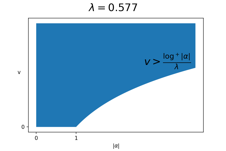
when λ > 0 𝜆 0 \lambda>0 ,
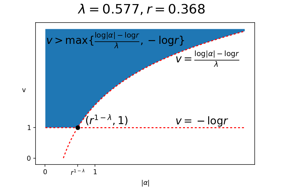
( z , w ) ∈ P α 𝑧 𝑤 subscript 𝑃 𝛼 \displaystyle(z,w)\in P_{\alpha} ⟺ v > log + | α | λ , ⟺ absent 𝑣 superscript 𝛼 𝜆 \displaystyle\Longleftrightarrow v>\frac{\log^{+}|\alpha|}{\lambda},
( z , w ) ∈ P α ( r ) 𝑧 𝑤 superscript subscript 𝑃 𝛼 𝑟 \displaystyle(z,w)\in P_{\alpha}^{(r)} ⟺ { v > log | α | − log r λ ( | α | ⩾ r 1 − λ ) , v > − log r ( | α | < r 1 − λ ) . \displaystyle\Longleftrightarrow\left\{\begin{aligned} &v>\frac{\log|\alpha|-\log r}{\lambda}&\quad{\scriptstyle{(|\alpha|\geqslant r^{1-\lambda})}},\\
&v>-\log r&\quad{\scriptstyle{(|\alpha|<r^{1-\lambda})}}.\end{aligned}\right.
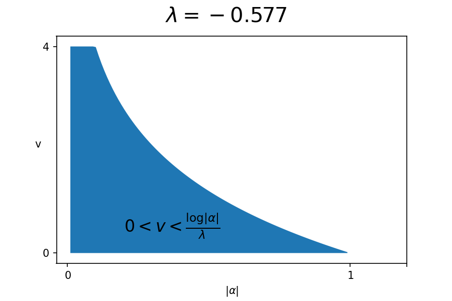
2.
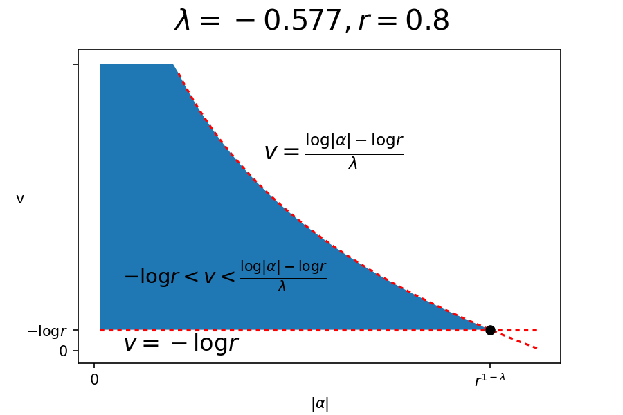
when λ < 0 𝜆 0 \lambda<0 , P α = ∅ subscript 𝑃 𝛼 P_{\alpha}=\emptyset for | α | ⩾ 1 𝛼 1 |\alpha|\geqslant 1 , P α ( r ) = ∅ superscript subscript 𝑃 𝛼 𝑟 P_{\alpha}^{(r)}=\emptyset for | α | ⩾ r 1 − λ 𝛼 superscript 𝑟 1 𝜆 |\alpha|\geqslant r^{1-\lambda} and for the other α 𝛼 \alpha
( z , w ) ∈ P α 𝑧 𝑤 subscript 𝑃 𝛼 \displaystyle(z,w)\in P_{\alpha} ⟺ 0 < v < log | α | λ , ⟺ absent 0 𝑣 𝛼 𝜆 \displaystyle\Longleftrightarrow 0<v<\frac{\log|\alpha|}{\lambda},
( z , w ) ∈ P α ( r ) 𝑧 𝑤 superscript subscript 𝑃 𝛼 𝑟 \displaystyle(z,w)\in P_{\alpha}^{(r)} ⟺ − log r < v < log | α | − log r λ . ⟺ absent 𝑟 𝑣 𝛼 𝑟 𝜆 \displaystyle\Longleftrightarrow-\log r<v<\frac{\log|\alpha|-\log r}{\lambda}.
Proof.
Recall that ( z , w ) = ( e − v + i u , α e − λ v + i λ u ) 𝑧 𝑤 superscript 𝑒 𝑣 𝑖 𝑢 𝛼 superscript 𝑒 𝜆 𝑣 𝑖 𝜆 𝑢 (z,w)=(e^{-v+i\,u},\alpha\,e^{-\lambda\,v+i\,\lambda\,u}) L α subscript 𝐿 𝛼 L_{\alpha} r ∈ ( 0 , 1 ] 𝑟 0 1 r\in(0,1] ( z , w ) ∈ P α ( r ) 𝑧 𝑤 superscript subscript 𝑃 𝛼 𝑟 (z,w)\in P_{\alpha}^{(r)} | z | = e − v < r 𝑧 superscript 𝑒 𝑣 𝑟 |z|=e^{-v}<r | w | = | α | e − λ v < r 𝑤 𝛼 superscript 𝑒 𝜆 𝑣 𝑟 |w|=|\alpha|\,e^{-\lambda\,v}<r
When λ > 0 𝜆 0 \lambda>0 v > − log r 𝑣 𝑟 v>-\log r v > log | α | − log r λ 𝑣 𝛼 𝑟 𝜆 v>\frac{\log|\alpha|-\log r}{\lambda} r = 1 𝑟 1 r=1 v > 0 𝑣 0 v>0 v > log | α | λ 𝑣 𝛼 𝜆 v>\frac{\log|\alpha|}{\lambda}
When λ < 0 𝜆 0 \lambda<0 − log r < v < log | α | − log r λ 𝑟 𝑣 𝛼 𝑟 𝜆 -\log r<v<\frac{\log|\alpha|-\log r}{\lambda} r = 1 𝑟 1 r=1 0 < v < log | α | λ 0 𝑣 𝛼 𝜆 0<v<\frac{\log|\alpha|}{\lambda} v 𝑣 v P α ( r ) = ∅ superscript subscript 𝑃 𝛼 𝑟 P_{\alpha}^{(r)}=\emptyset
When λ > 0 𝜆 0 \lambda>0 v 𝑣 v α ∈ ℂ ∗ 𝛼 superscript ℂ \alpha\in\mathbb{C}^{*}
Figure 1: The region of ( | α | , v ) 𝛼 𝑣 (|\alpha|,v) P α subscript 𝑃 𝛼 P_{\alpha} Figure 2: The region of ( | α | , v ) 𝛼 𝑣 (|\alpha|,v) P α ( r ) superscript subscript 𝑃 𝛼 𝑟 P_{\alpha}^{(r)}
When λ < 0 𝜆 0 \lambda<0 v 𝑣 v α 𝛼 \alpha
Figure 3: The region of ( | α | , v ) 𝛼 𝑣 (|\alpha|,v) P α subscript 𝑃 𝛼 P_{\alpha} Figure 4: The region of ( | α | , v ) 𝛼 𝑣 (|\alpha|,v) P α ( r ) superscript subscript 𝑃 𝛼 𝑟 P_{\alpha}^{(r)}
In this article, the notations ≲ less-than-or-similar-to \lesssim ≳ greater-than-or-equivalent-to \gtrsim λ 𝜆 \lambda ≈ \approx
3 Geometry of leaves when λ > 0 𝜆 0 \lambda>0
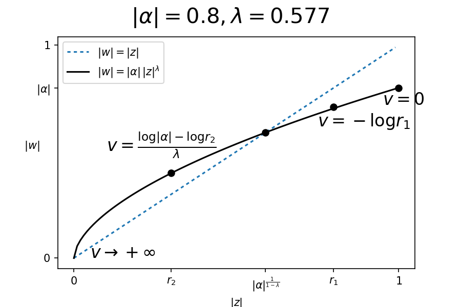
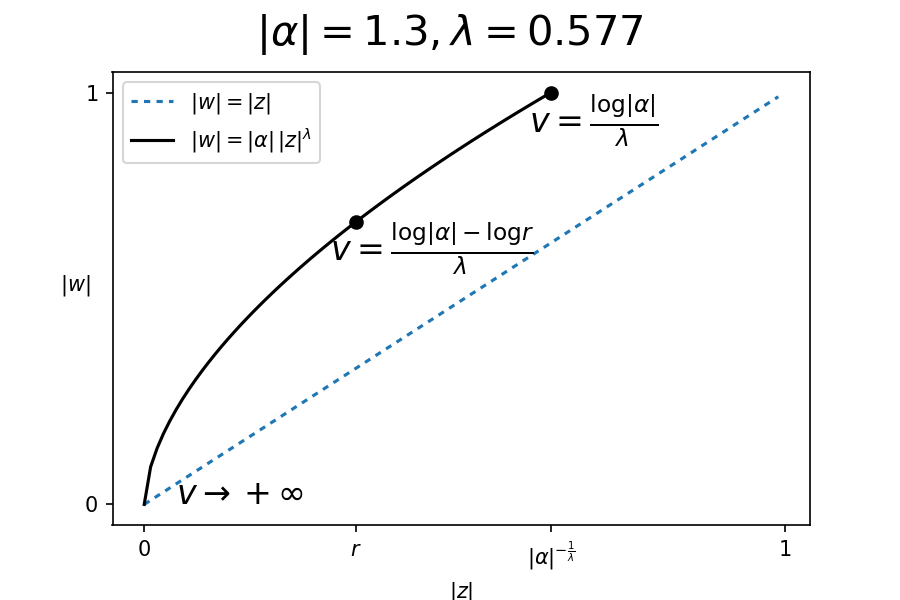
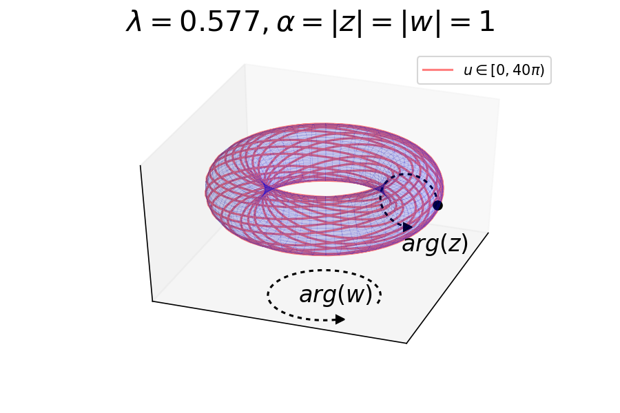
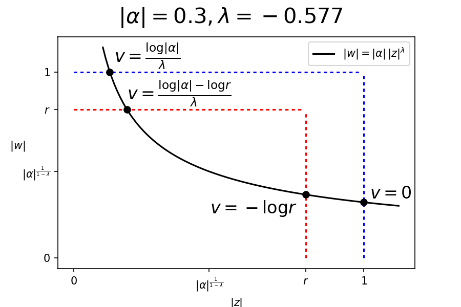
For any α ∈ ℂ ∗ 𝛼 superscript ℂ \alpha\in\mathbb{C}^{*} L α subscript 𝐿 𝛼 L_{\alpha} | w | = | α | | z | λ 𝑤 𝛼 superscript 𝑧 𝜆 |w|=|\alpha|\,|z|^{\lambda} | z | = e − v 𝑧 superscript 𝑒 𝑣 |z|=e^{-v} | w | = | α | e − λ v 𝑤 𝛼 superscript 𝑒 𝜆 𝑣 |w|=|\alpha|\,e^{-\lambda v} | z | 𝑧 |z| | w | 𝑤 |w| v 𝑣 v v → + ∞ → 𝑣 v\rightarrow+\infty ( 0 , 0 ) 0 0 (0,0)
Figure 5: Case | α | < 1 𝛼 1 |\alpha|<1 Figure 6: Case | α | ⩾ 1 𝛼 1 |\alpha|\geqslant 1
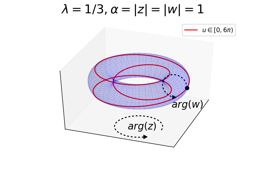
If one fixes some v = − log r 𝑣 𝑟 v=-\log r | z | = r 𝑧 𝑟 |z|=r | w | = | α | r λ 𝑤 𝛼 superscript 𝑟 𝜆 |w|=|\alpha|\,r^{\lambda} 𝕋 r 2 := { ( z , w ) ∈ 𝔻 2 : | z | = r , | w | = | α | r λ } assign subscript superscript 𝕋 2 𝑟 conditional-set 𝑧 𝑤 superscript 𝔻 2 formulae-sequence 𝑧 𝑟 𝑤 𝛼 superscript 𝑟 𝜆 \mathbb{T}^{2}_{r}:=\{(z,w)\in\mathbb{D}^{2}~{}:~{}|z|=r,|w|=|\alpha|\,r^{\lambda}\} L α subscript 𝐿 𝛼 L_{\alpha} L α , r := L α ∩ 𝕋 r 2 assign subscript 𝐿 𝛼 𝑟
subscript 𝐿 𝛼 subscript superscript 𝕋 2 𝑟 L_{\alpha,r}:=L_{\alpha}\cap\mathbb{T}^{2}_{r}
When λ ∈ ℚ 𝜆 ℚ \lambda\in\mathbb{Q} L α , r subscript 𝐿 𝛼 𝑟
L_{\alpha,r}
Figure 7: a closed curve on a torus
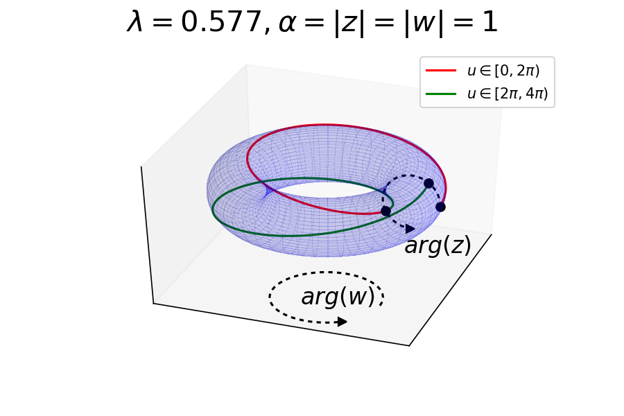
When λ ∉ ℚ 𝜆 ℚ \lambda\notin\mathbb{Q} L α , r subscript 𝐿 𝛼 𝑟
L_{\alpha,r} 𝕋 r 2 superscript subscript 𝕋 𝑟 2 \mathbb{T}_{r}^{2}
Figure 8: 2 loopsFigure 9: 20 loops
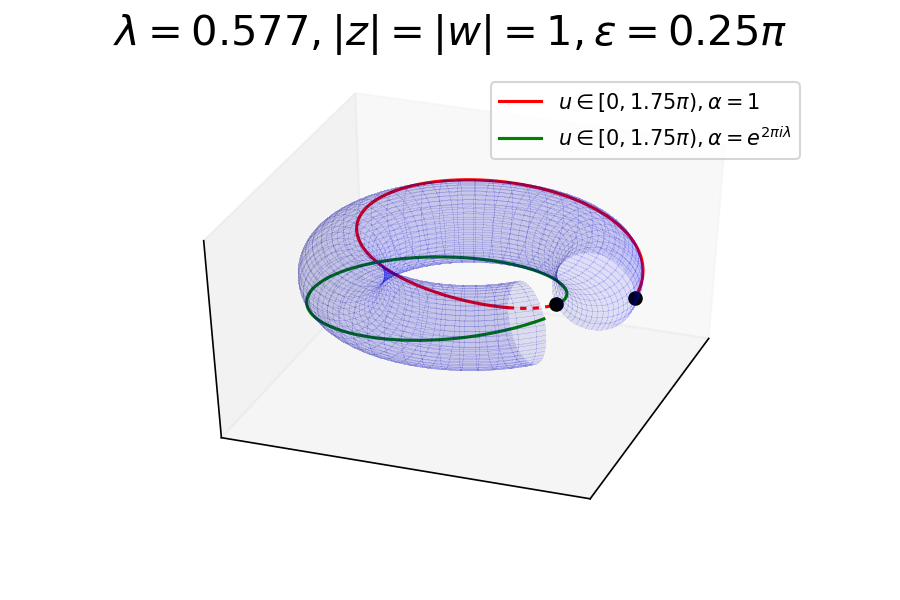
In this case the two curves L α , r subscript 𝐿 𝛼 𝑟
L_{\alpha,r} L α e 2 π i λ , r subscript 𝐿 𝛼 superscript 𝑒 2 𝜋 𝑖 𝜆 𝑟
L_{\alpha\,e^{2\pi i\lambda},r} 8 L α , r subscript 𝐿 𝛼 𝑟
L_{\alpha,r} u ∈ [ 2 π , 4 π ) 𝑢 2 𝜋 4 𝜋 u\in[2\pi,4\pi) L α e 2 π i λ , r subscript 𝐿 𝛼 superscript 𝑒 2 𝜋 𝑖 𝜆 𝑟
L_{\alpha\,e^{2\pi i\lambda},r} u ∈ [ 0 , 2 π ) 𝑢 0 2 𝜋 u\in[0,2\pi) L α subscript 𝐿 𝛼 L_{\alpha}
Such ambiguity can be resolved once one restricts everything to an open subset U ϵ := { ( z , w ) ∈ 𝔻 2 | arg ( z ) ∈ ( 0 , 2 π − ϵ ) , z ≠ 0 , w ≠ 0 } assign subscript 𝑈 italic-ϵ conditional-set 𝑧 𝑤 superscript 𝔻 2 formulae-sequence arg 𝑧 0 2 𝜋 italic-ϵ formulae-sequence 𝑧 0 𝑤 0 U_{\epsilon}:=\{(z,w)\in\mathbb{D}^{2}~{}|~{}{\rm arg}(z)\in(0,2\pi-\epsilon),z\neq 0,w\neq 0\} ϵ ∈ [ 0 , π ) italic-ϵ 0 𝜋 \epsilon\in[0,\pi) L α subscript 𝐿 𝛼 L_{\alpha} U ϵ subscript 𝑈 italic-ϵ U_{\epsilon}
L α ∩ U ϵ = ⋃ k ∈ ℤ { ( e − v + i u , α e 2 k π i λ e − λ v + i λ u ) | u ∈ ( 0 , 2 π − ϵ ) , v > log + | α | λ } . subscript 𝐿 𝛼 subscript 𝑈 italic-ϵ subscript 𝑘 ℤ conditional-set superscript 𝑒 𝑣 𝑖 𝑢 𝛼 superscript 𝑒 2 𝑘 𝜋 𝑖 𝜆 superscript 𝑒 𝜆 𝑣 𝑖 𝜆 𝑢 formulae-sequence 𝑢 0 2 𝜋 italic-ϵ 𝑣 superscript 𝛼 𝜆 L_{\alpha}\cap U_{\epsilon}=\bigcup\limits_{k\in\mathbb{Z}}\big{\{}(e^{-v+iu},\alpha\,e^{2k\pi i\lambda}\,e^{-\lambda v+i\lambda u})~{}|~{}u\in(0,2\pi-\epsilon),v>\textstyle\frac{\log^{+}|\alpha|}{\lambda}\big{\}}.
Such a parametrization is yet not unique. For example for any k 0 ∈ ℤ subscript 𝑘 0 ℤ k_{0}\in\mathbb{Z}
L α ∩ U ϵ = ⋃ k ∈ ℤ { ( e − v + i u , α e 2 k π i λ e − λ v + i λ u ) | u ∈ ( 2 k 0 π , 2 k 0 π + 2 π − ϵ ) , v > log + | α | λ } . subscript 𝐿 𝛼 subscript 𝑈 italic-ϵ subscript 𝑘 ℤ conditional-set superscript 𝑒 𝑣 𝑖 𝑢 𝛼 superscript 𝑒 2 𝑘 𝜋 𝑖 𝜆 superscript 𝑒 𝜆 𝑣 𝑖 𝜆 𝑢 formulae-sequence 𝑢 2 subscript 𝑘 0 𝜋 2 subscript 𝑘 0 𝜋 2 𝜋 italic-ϵ 𝑣 superscript 𝛼 𝜆 L_{\alpha}\cap U_{\epsilon}=\bigcup\limits_{k\in\mathbb{Z}}\big{\{}(e^{-v+iu},\alpha\,e^{2k\pi i\lambda}\,e^{-\lambda v+i\lambda u})~{}|~{}u\in(2k_{0}\pi,2k_{0}\pi+2\pi-\epsilon),v>\textstyle\frac{\log^{+}|\alpha|}{\lambda}\big{\}}.
The parametrization is unique once one fixes k 0 subscript 𝑘 0 k_{0} k 0 = 0 subscript 𝑘 0 0 k_{0}=0 k 0 subscript 𝑘 0 k_{0}
Once one specifies the range of u 𝑢 u k 0 = 0 subscript 𝑘 0 0 k_{0}=0 U ϵ subscript 𝑈 italic-ϵ U_{\epsilon}
Figure 10: The curve L 1 , 1 subscript 𝐿 1 1
L_{1,1} L e 2 π i λ , 1 subscript 𝐿 superscript 𝑒 2 𝜋 𝑖 𝜆 1
L_{e^{2\pi i\lambda},1}
Later the limit case when ϵ = 0 italic-ϵ 0 \epsilon=0 U := { ( z , w ) ∈ 𝔻 2 | arg ( z ) ∈ ( 0 , 2 π ) , z ≠ 0 , w ≠ 0 } = { ( z , w ) ∈ 𝔻 2 | z ∉ ℝ ⩾ 0 , w ≠ 0 } assign 𝑈 conditional-set 𝑧 𝑤 superscript 𝔻 2 formulae-sequence arg 𝑧 0 2 𝜋 formulae-sequence 𝑧 0 𝑤 0 conditional-set 𝑧 𝑤 superscript 𝔻 2 formulae-sequence 𝑧 subscript ℝ absent 0 𝑤 0 U:=\{(z,w)\in\mathbb{D}^{2}~{}|~{}{\rm arg}(z)\in(0,2\pi),z\neq 0,w\neq 0\}=\{(z,w)\in\mathbb{D}^{2}~{}|~{}z\notin\mathbb{R}_{\geqslant 0},w\neq 0\}
4 Rational case: λ = a b ∈ ℚ 𝜆 𝑎 𝑏 ℚ \lambda=\frac{a}{b}\in\mathbb{Q} λ ∈ ( 0 , 1 ] 𝜆 0 1 \lambda\in(0,1]
Say λ = a b 𝜆 𝑎 𝑏 \lambda=\frac{a}{b} a , b ∈ ℤ ⩾ 1 𝑎 𝑏
subscript ℤ absent 1 a,b\in\mathbb{Z}_{\geqslant 1} 𝔻 2 superscript 𝔻 2 \mathbb{D}^{2} α ∈ ℂ ∗ 𝛼 superscript ℂ \alpha\in\mathbb{C}^{*} L α ∪ { 0 } subscript 𝐿 𝛼 0 L_{\alpha}\cup\{0\} { w b = α b z a } ∩ 𝔻 2 superscript 𝑤 𝑏 superscript 𝛼 𝑏 superscript 𝑧 𝑎 superscript 𝔻 2 \{w^{b}=\alpha^{b}\,z^{a}\}\cap\mathbb{D}^{2} T 𝑇 T
The parametrization map ψ α ( ζ ) := ( e i ζ , α e i λ ζ ) assign subscript 𝜓 𝛼 𝜁 superscript 𝑒 𝑖 𝜁 𝛼 superscript 𝑒 𝑖 𝜆 𝜁 \psi_{\alpha}(\zeta):=(e^{i\zeta},\alpha\,e^{i\lambda\zeta}) ψ α ( ζ + 2 π b ) = ψ α ( ζ ) subscript 𝜓 𝛼 𝜁 2 𝜋 𝑏 subscript 𝜓 𝛼 𝜁 \psi_{\alpha}(\zeta+2\pi b)=\psi_{\alpha}(\zeta) T 𝑇 T T | P α evaluated-at 𝑇 subscript 𝑃 𝛼 T|_{P_{\alpha}} h α ( z , w ) [ P α ] subscript ℎ 𝛼 𝑧 𝑤 delimited-[] subscript 𝑃 𝛼 h_{\alpha}(z,w)[P_{\alpha}]
H α ( u + i v ) := h α ∘ ψ α ( u + i v + i log + | α | λ ) . assign subscript 𝐻 𝛼 𝑢 𝑖 𝑣 subscript ℎ 𝛼 subscript 𝜓 𝛼 𝑢 𝑖 𝑣 𝑖 superscript 𝛼 𝜆 H_{\alpha}(u+iv):=h_{\alpha}\circ\psi_{\alpha}\big{(}u+iv+i\frac{\log^{+}|\alpha|}{\lambda}\big{)}.
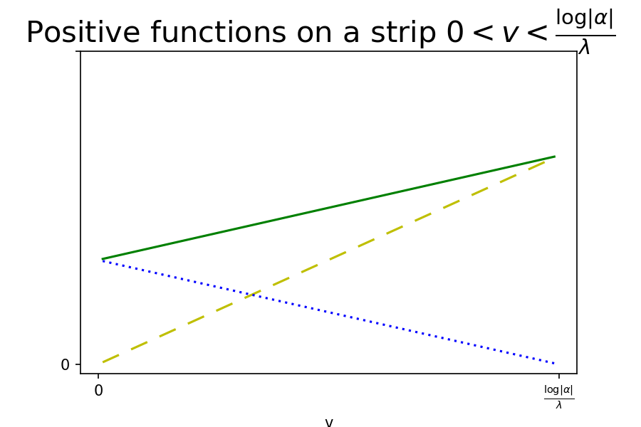
It is a positive harmonic function for μ 𝜇 \mu α ∈ ℂ ∗ 𝛼 superscript ℂ \alpha\in\mathbb{C}^{*} ℍ := { ( u + i v ) ∈ ℂ | v > 0 } assign ℍ conditional-set 𝑢 𝑖 𝑣 ℂ 𝑣 0 \mathbb{H}:=\{(u+iv)\in\mathbb{C}~{}|~{}v>0\} H α ( u + i v ) = H α ( u + 2 π b + i v ) subscript 𝐻 𝛼 𝑢 𝑖 𝑣 subscript 𝐻 𝛼 𝑢 2 𝜋 𝑏 𝑖 𝑣 H_{\alpha}(u+iv)=H_{\alpha}(u+2\pi b+iv)
Lemma 4.1 .
Let F ( u , v ) 𝐹 𝑢 𝑣 F(u,v) ℍ ℍ \mathbb{H} F ( u , v ) = F ( u + 2 π b , v ) 𝐹 𝑢 𝑣 𝐹 𝑢 2 𝜋 𝑏 𝑣 F(u,v)=F(u+2\pi b,v) ( u , v ) ∈ ℍ 𝑢 𝑣 ℍ (u,v)\in\mathbb{H}
F ( u , v ) = ∑ k ∈ ℤ , k ≠ 0 ( a k e k v b cos ( k u b ) + b k e k v b sin ( k u b ) ) + a 0 + b 0 v , 𝐹 𝑢 𝑣 subscript formulae-sequence 𝑘 ℤ 𝑘 0 subscript 𝑎 𝑘 superscript 𝑒 𝑘 𝑣 𝑏 𝑘 𝑢 𝑏 subscript 𝑏 𝑘 superscript 𝑒 𝑘 𝑣 𝑏 𝑘 𝑢 𝑏 subscript 𝑎 0 subscript 𝑏 0 𝑣 F(u,v)=\sum\limits_{k\in\mathbb{Z},k\neq 0}\big{(}a_{k}\,e^{\frac{kv}{b}}\cos(\textstyle\frac{ku}{b})+b_{k}\,e^{\frac{kv}{b}}\sin(\frac{ku}{b})\big{)}+a_{0}+b_{0}\,v,
for some a k subscript 𝑎 𝑘 a_{k} b k ∈ ℝ subscript 𝑏 𝑘 ℝ b_{k}\in\mathbb{R} F | ℍ ⩾ 0 evaluated-at 𝐹 ℍ 0 F|_{\mathbb{H}}\geqslant 0 a 0 , b 0 ⩾ 0 subscript 𝑎 0 subscript 𝑏 0
0 a_{0},b_{0}\geqslant 0
Proof.
By periodicity
F ( u , v ) = ∑ k = 1 ∞ ( A k ( v ) cos ( k u b ) + B k ( v ) sin ( k u b ) ) + A 0 ( v ) , 𝐹 𝑢 𝑣 superscript subscript 𝑘 1 subscript 𝐴 𝑘 𝑣 𝑘 𝑢 𝑏 subscript 𝐵 𝑘 𝑣 𝑘 𝑢 𝑏 subscript 𝐴 0 𝑣 F(u,v)=\sum\limits_{k=1}^{\infty}\big{(}A_{k}(v)\,\cos(\textstyle\frac{ku}{b})+B_{k}(v)\,\sin(\frac{ku}{b})\big{)}+A_{0}(v),
for some functions A k ( v ) subscript 𝐴 𝑘 𝑣 A_{k}(v) B k ( v ) subscript 𝐵 𝑘 𝑣 B_{k}(v) F 𝐹 F
0 = Δ F ( u , v ) = ∑ k = 1 ∞ ( ( A k ′′ ( v ) − ( k b ) 2 A k ( v ) ) cos ( k u b ) + ( B k ′′ ( v ) − ( k b ) 2 B k ( v ) ) sin ( k u b ) ) + A 0 ′′ ( v ) . 0 Δ 𝐹 𝑢 𝑣 superscript subscript 𝑘 1 superscript subscript 𝐴 𝑘 ′′ 𝑣 superscript 𝑘 𝑏 2 subscript 𝐴 𝑘 𝑣 𝑘 𝑢 𝑏 superscript subscript 𝐵 𝑘 ′′ 𝑣 superscript 𝑘 𝑏 2 subscript 𝐵 𝑘 𝑣 𝑘 𝑢 𝑏 superscript subscript 𝐴 0 ′′ 𝑣 0=\Delta F(u,v)=\sum\limits_{k=1}^{\infty}\Big{(}\big{(}A_{k}^{\prime\prime}(v)-(\textstyle\frac{k}{b})^{2}\,A_{k}(v)\big{)}\,\cos(\frac{ku}{b})+\big{(}B_{k}^{\prime\prime}(v)-(\frac{k}{b})^{2}\,B_{k}(v)\big{)}\,\sin(\frac{ku}{b})\Big{)}+A_{0}^{\prime\prime}(v).
Thus
A k ′′ ( v ) = ( k b ) 2 A k ( v ) , B k ′′ ( v ) = ( k b ) 2 B k ( v ) , A 0 ′′ ( v ) = 0 . formulae-sequence superscript subscript 𝐴 𝑘 ′′ 𝑣 superscript 𝑘 𝑏 2 subscript 𝐴 𝑘 𝑣 formulae-sequence superscript subscript 𝐵 𝑘 ′′ 𝑣 superscript 𝑘 𝑏 2 subscript 𝐵 𝑘 𝑣 superscript subscript 𝐴 0 ′′ 𝑣 0 A_{k}^{\prime\prime}(v)=(\textstyle\frac{k}{b})^{2}\,A_{k}(v),\ \ \ \ B_{k}^{\prime\prime}(v)=(\frac{k}{b})^{2}\,B_{k}(v),\ \ \ \ A_{0}^{\prime\prime}(v)=0.
Hence
A k ( v ) = a k e k v b + a − k e − k v b , B k ( v ) = b k e k v b − b − k e − k v b , A 0 ( v ) = a 0 + b 0 v , formulae-sequence subscript 𝐴 𝑘 𝑣 subscript 𝑎 𝑘 superscript 𝑒 𝑘 𝑣 𝑏 subscript 𝑎 𝑘 superscript 𝑒 𝑘 𝑣 𝑏 formulae-sequence subscript 𝐵 𝑘 𝑣 subscript 𝑏 𝑘 superscript 𝑒 𝑘 𝑣 𝑏 subscript 𝑏 𝑘 superscript 𝑒 𝑘 𝑣 𝑏 subscript 𝐴 0 𝑣 subscript 𝑎 0 subscript 𝑏 0 𝑣 A_{k}(v)=a_{k}\,e^{\frac{kv}{b}}+a_{-k}\,e^{-\frac{kv}{b}},\ \ \ \ B_{k}(v)=b_{k}\,e^{\frac{kv}{b}}-b_{-k}\,e^{-\frac{kv}{b}},\ \ \ \ A_{0}(v)=a_{0}+b_{0}\,v,
for some a k subscript 𝑎 𝑘 a_{k} a − k subscript 𝑎 𝑘 a_{-k} b k subscript 𝑏 𝑘 b_{k} b − k ∈ ℝ subscript 𝑏 𝑘 ℝ b_{-k}\in\mathbb{R}
If F | ℍ ⩾ 0 evaluated-at 𝐹 ℍ 0 F|_{\mathbb{H}}\geqslant 0 v ⩾ 0 𝑣 0 v\geqslant 0
∫ u = 0 2 π b F ( u , v ) 𝑑 u = 2 π b ( a 0 + b 0 v ) ⩾ 0 . superscript subscript 𝑢 0 2 𝜋 𝑏 𝐹 𝑢 𝑣 differential-d 𝑢 2 𝜋 𝑏 subscript 𝑎 0 subscript 𝑏 0 𝑣 0 \int_{u=0}^{2\pi b}F(u,v)du=2\pi b(a_{0}+b_{0}\,v)\geqslant 0.
Thus a 0 , b 0 ⩾ 0 . subscript 𝑎 0 subscript 𝑏 0
0 a_{0},b_{0}\geqslant 0.
For α , β ∈ ℂ ∗ 𝛼 𝛽
superscript ℂ \alpha,\beta\in\mathbb{C}^{*} ψ α subscript 𝜓 𝛼 \psi_{\alpha} ψ β subscript 𝜓 𝛽 \psi_{\beta} L α = L β subscript 𝐿 𝛼 subscript 𝐿 𝛽 L_{\alpha}=L_{\beta} β = α e 2 π i k b 𝛽 𝛼 superscript 𝑒 2 𝜋 𝑖 𝑘 𝑏 \beta=\alpha\,e^{2\pi i\frac{k}{b}} k ∈ ℤ 𝑘 ℤ k\in\mathbb{Z} α 𝛼 \alpha β 𝛽 \beta b 𝑡ℎ superscript 𝑏 𝑡ℎ b^{\sl th} 𝕋 := { α ∈ ℂ ∗ | arg ( α ) ∈ [ 0 , 2 π b ) } assign 𝕋 conditional-set 𝛼 superscript ℂ arg 𝛼 0 2 𝜋 𝑏 \mathbb{T}:=\{\alpha\in\mathbb{C}^{*}~{}|~{}{\rm arg}(\alpha)\in[0,\frac{2\pi}{b})\} H α ( 0 ) = h α ∘ ψ α ( i log + | α | λ ) = 1 subscript 𝐻 𝛼 0 subscript ℎ 𝛼 subscript 𝜓 𝛼 𝑖 superscript 𝛼 𝜆 1 H_{\alpha}(0)=h_{\alpha}\circ\psi_{\alpha}(i\frac{\log^{+}|\alpha|}{\lambda})=1
The mass of the current T 𝑇 T
‖ T ‖ 𝔻 2 = ∫ ( z , w ) ∈ 𝔻 2 T ∧ i ∂ ∂ ¯ ( | z | 2 + | w | 2 ) . subscript norm 𝑇 superscript 𝔻 2 subscript 𝑧 𝑤 superscript 𝔻 2 𝑇 𝑖 ¯ superscript 𝑧 2 superscript 𝑤 2 |\!\!|T|\!\!|_{\mathbb{D}^{2}}=\int_{(z,w)\in\mathbb{D}^{2}}T\wedge i\partial\bar{\partial}(|z|^{2}+|w|^{2}).
In particular, one calculates the ( 1 , 1 ) 1 1 (1,1) i ∂ ∂ ¯ ( | z | 2 + | w | 2 ) 𝑖 ¯ superscript 𝑧 2 superscript 𝑤 2 i\partial\bar{\partial}(|z|^{2}+|w|^{2}) L α subscript 𝐿 𝛼 L_{\alpha} z = e − v + i u , w = α e − λ v + i λ u formulae-sequence 𝑧 superscript 𝑒 𝑣 𝑖 𝑢 𝑤 𝛼 superscript 𝑒 𝜆 𝑣 𝑖 𝜆 𝑢 z=e^{-v+iu},w=\alpha\,e^{-\lambda v+i\lambda u}
d z 𝑑 𝑧 \displaystyle dz = i e − v + i u d u − e − v + i u d v , absent 𝑖 superscript 𝑒 𝑣 𝑖 𝑢 𝑑 𝑢 superscript 𝑒 𝑣 𝑖 𝑢 𝑑 𝑣 \displaystyle=ie^{-v+iu}du-e^{-v+iu}dv, d z ¯ 𝑑 ¯ 𝑧 \displaystyle d\bar{z} = − i e − v − i u d u − e − v − i u d v , absent 𝑖 superscript 𝑒 𝑣 𝑖 𝑢 𝑑 𝑢 superscript 𝑒 𝑣 𝑖 𝑢 𝑑 𝑣 \displaystyle=-ie^{-v-iu}du-e^{-v-iu}dv,
d w 𝑑 𝑤 \displaystyle dw = i α λ e − λ v + i λ u d u − α λ e − λ v + i λ u d v , absent 𝑖 𝛼 𝜆 superscript 𝑒 𝜆 𝑣 𝑖 𝜆 𝑢 𝑑 𝑢 𝛼 𝜆 superscript 𝑒 𝜆 𝑣 𝑖 𝜆 𝑢 𝑑 𝑣 \displaystyle=i\alpha\,\lambda\,e^{-\lambda\,v+i\lambda\,u}du-\alpha\,\lambda\,e^{-\lambda\,v+i\lambda\,u}dv, d w ¯ 𝑑 ¯ 𝑤 \displaystyle d\bar{w} = − i α ¯ λ e − λ v − i λ u d u − α ¯ λ e − λ v − i λ u d v , absent 𝑖 ¯ 𝛼 𝜆 superscript 𝑒 𝜆 𝑣 𝑖 𝜆 𝑢 𝑑 𝑢 ¯ 𝛼 𝜆 superscript 𝑒 𝜆 𝑣 𝑖 𝜆 𝑢 𝑑 𝑣 \displaystyle=-i\bar{\alpha}\,\lambda\,e^{-\lambda\,v-i\lambda\,u}du-\bar{\alpha}\,\lambda\,e^{-\lambda\,v-i\lambda\,u}dv,
whence
i ∂ ∂ ¯ ( | z | 2 + | w | 2 ) 𝑖 ¯ superscript 𝑧 2 superscript 𝑤 2 \displaystyle i\partial\bar{\partial}(|z|^{2}+|w|^{2}) = i d z ∧ d z ¯ + i d w ∧ d w ¯ absent 𝑖 𝑑 𝑧 𝑑 ¯ 𝑧 𝑖 𝑑 𝑤 𝑑 ¯ 𝑤 \displaystyle=idz\wedge d\bar{z}+idw\wedge d\bar{w}
= 2 ( e − 2 v + λ 2 | α | 2 e − 2 λ v ) d u ∧ d v . absent 2 superscript 𝑒 2 𝑣 superscript 𝜆 2 superscript 𝛼 2 superscript 𝑒 2 𝜆 𝑣 𝑑 𝑢 𝑑 𝑣 \displaystyle=2\big{(}e^{-2v}+\lambda^{2}\,|\alpha|^{2}\,e^{-2\lambda\,v}\big{)}du\wedge dv.
Thus
‖ T ‖ 𝔻 2 subscript norm 𝑇 superscript 𝔻 2 \displaystyle|\!|T|\!|_{\mathbb{D}^{2}} = ∫ α ∈ 𝕋 h α ( z , w ) ∫ P α i ∂ ∂ ¯ ( | z | 2 + | w | 2 ) d μ ( α ) absent subscript 𝛼 𝕋 subscript ℎ 𝛼 𝑧 𝑤 subscript subscript 𝑃 𝛼 𝑖 ¯ superscript 𝑧 2 superscript 𝑤 2 𝑑 𝜇 𝛼 \displaystyle=\int_{\alpha\in\mathbb{T}}h_{\alpha}(z,w)\int_{P_{\alpha}}i\partial\bar{\partial}(|z|^{2}+|w|^{2})\,d\mu(\alpha)
= ∫ α ∈ 𝕋 ∫ u = 0 2 π b ∫ v > 0 H α ( u + i v ) 2 ( e − 2 ( v + log + | α | λ ) + λ 2 | α | 2 e − 2 λ ( v + log + | α | λ ) ) 𝑑 u ∧ d v d μ ( α ) absent subscript 𝛼 𝕋 superscript subscript 𝑢 0 2 𝜋 𝑏 subscript 𝑣 0 subscript 𝐻 𝛼 𝑢 𝑖 𝑣 2 superscript 𝑒 2 𝑣 superscript 𝛼 𝜆 superscript 𝜆 2 superscript 𝛼 2 superscript 𝑒 2 𝜆 𝑣 superscript 𝛼 𝜆 differential-d 𝑢 𝑑 𝑣 𝑑 𝜇 𝛼 \displaystyle=\int_{\alpha\in\mathbb{T}}\int_{u=0}^{2\pi b}\int_{v>0}H_{\alpha}(u+iv)\,2\big{(}e^{-2(v+\frac{\log^{+}|\alpha|}{\lambda})}+\lambda^{2}\,|\alpha|^{2}\,e^{-2\lambda\,(v+\frac{\log^{+}|\alpha|}{\lambda})}\big{)}\,du\wedge dv\,d\mu(\alpha)
= ∫ α ∈ 𝕋 , | α | < 1 ∫ u = 0 2 π b ∫ v > 0 H α ( u + i v ) 2 ( e − 2 v + λ 2 | α | 2 e − 2 λ v ) 𝑑 u ∧ d v d μ ( α ) absent subscript formulae-sequence 𝛼 𝕋 𝛼 1 superscript subscript 𝑢 0 2 𝜋 𝑏 subscript 𝑣 0 subscript 𝐻 𝛼 𝑢 𝑖 𝑣 2 superscript 𝑒 2 𝑣 superscript 𝜆 2 superscript 𝛼 2 superscript 𝑒 2 𝜆 𝑣 differential-d 𝑢 𝑑 𝑣 𝑑 𝜇 𝛼 \displaystyle=\int_{\alpha\in\mathbb{T},|\alpha|<1}\int_{u=0}^{2\pi b}\int_{v>0}H_{\alpha}(u+iv)\,2\big{(}e^{-2v}+\lambda^{2}\,|\alpha|^{2}\,e^{-2\lambda\,v}\big{)}\,du\wedge dv\,d\mu(\alpha)
+ ∫ α ∈ 𝕋 , | α | ⩾ 1 ∫ u = 0 2 π b ∫ v > 0 H α ( u + i v ) 2 ( | α | − 2 λ e − 2 v + λ 2 e − 2 λ v ) 𝑑 u ∧ d v d μ ( α ) . subscript formulae-sequence 𝛼 𝕋 𝛼 1 superscript subscript 𝑢 0 2 𝜋 𝑏 subscript 𝑣 0 subscript 𝐻 𝛼 𝑢 𝑖 𝑣 2 superscript 𝛼 2 𝜆 superscript 𝑒 2 𝑣 superscript 𝜆 2 superscript 𝑒 2 𝜆 𝑣 differential-d 𝑢 𝑑 𝑣 𝑑 𝜇 𝛼 \displaystyle\ \ \ +\int_{\alpha\in\mathbb{T},|\alpha|\geqslant 1}\int_{u=0}^{2\pi b}\int_{v>0}H_{\alpha}(u+iv)\,2\big{(}|\alpha|^{-\frac{2}{\lambda}}\,e^{-2v}+\lambda^{2}\,e^{-2\lambda\,v}\big{)}du\wedge dv\,d\mu(\alpha).
By Lemma 4.1
H α ( u + i v ) = ∑ k ∈ ℤ , k ≠ 0 ( a k ( α ) e k v b cos ( k u b ) + b k ( α ) e k v b sin ( k u b ) ) + a 0 ( α ) + b 0 ( α ) v , subscript 𝐻 𝛼 𝑢 𝑖 𝑣 subscript formulae-sequence 𝑘 ℤ 𝑘 0 subscript 𝑎 𝑘 𝛼 superscript 𝑒 𝑘 𝑣 𝑏 𝑘 𝑢 𝑏 subscript 𝑏 𝑘 𝛼 superscript 𝑒 𝑘 𝑣 𝑏 𝑘 𝑢 𝑏 subscript 𝑎 0 𝛼 subscript 𝑏 0 𝛼 𝑣 H_{\alpha}(u+iv)=\sum\limits_{k\in\mathbb{Z},k\neq 0}\big{(}a_{k}(\alpha)\,e^{\frac{kv}{b}}\cos(\textstyle\frac{ku}{b})+b_{k}(\alpha)\,e^{\frac{kv}{b}}\sin(\frac{ku}{b})\big{)}+a_{0}(\alpha)+b_{0}(\alpha)\,v, (2)
where a 0 ( α ) subscript 𝑎 0 𝛼 a_{0}(\alpha) b 0 ( α ) subscript 𝑏 0 𝛼 b_{0}(\alpha) μ 𝜇 \mu α 𝛼 \alpha
‖ T ‖ 𝔻 2 subscript norm 𝑇 superscript 𝔻 2 \displaystyle|\!|T|\!|_{\mathbb{D}^{2}} = 2 π b { ∫ α ∈ 𝕋 , | α | < 1 ∫ v > 0 ( a 0 ( α ) + b 0 ( α ) v ) 2 ( e − 2 v + λ 2 | α | 2 e − 2 λ v ) d v d μ ( α ) \displaystyle=2\pi b\Big{\{}\int_{\alpha\in\mathbb{T},|\alpha|<1}\int_{v>0}\big{(}a_{0}(\alpha)+b_{0}(\alpha)v\big{)}\,2(e^{-2v}+\lambda^{2}\,|\alpha|^{2}\,e^{-2\lambda\,v})\,dv\,d\mu(\alpha)
+ ∫ α ∈ 𝕋 , | α | ⩾ 1 ∫ v > 0 ( a 0 ( α ) + b 0 ( α ) v ) 2 ( | α | − 2 λ e − 2 v + λ 2 e − 2 λ v ) d v d μ ( α ) } \displaystyle\ \ \ \ \ \ \ +\int_{\alpha\in\mathbb{T},|\alpha|\geqslant 1}\int_{v>0}\big{(}a_{0}(\alpha)+b_{0}(\alpha)v\big{)}\,2(|\alpha|^{-\frac{2}{\lambda}}\,e^{-2v}+\lambda^{2}\,e^{-2\lambda\,v})\,dv\,d\mu(\alpha)\Big{\}}
= 2 π b { ∫ | α | < 1 a 0 ( α ) ( 1 + | α | 2 λ ) d μ ( α ) + ∫ | α | ⩾ 1 a 0 ( α ) ( | α | − 2 λ + λ ) d μ ( α ) \displaystyle=2\pi b\,\Big{\{}\int_{|\alpha|<1}a_{0}(\alpha)\,(1+|\alpha|^{2}\,\lambda)d\mu(\alpha)+\int_{|\alpha|\geqslant 1}a_{0}(\alpha)\,(|\alpha|^{-\frac{2}{\lambda}}+\lambda)d\mu(\alpha)
+ ∫ | α | < 1 b 0 ( α ) ( 1 2 + 1 2 | α | 2 ) d μ ( α ) + ∫ | α | ⩾ 1 b 0 ( α ) ( 1 2 + 1 2 | α | − 2 λ ) d μ ( α ) } \displaystyle\ \ \ \ \ \ +\int_{|\alpha|<1}b_{0}(\alpha)\,\big{(}\tfrac{1}{2}+\tfrac{1}{2}|\alpha|^{2}\big{)}d\mu(\alpha)+\int_{|\alpha|\geqslant 1}b_{0}(\alpha)\,\big{(}\tfrac{1}{2}+\tfrac{1}{2}|\alpha|^{-\frac{2}{\lambda}}\big{)}d\mu(\alpha)\Big{\}}
≈ ∫ α ∈ ℂ ∗ a 0 ( α ) 𝑑 μ ( α ) + ∫ α ∈ ℂ ∗ b 0 ( α ) 𝑑 μ ( α ) . absent subscript 𝛼 superscript ℂ subscript 𝑎 0 𝛼 differential-d 𝜇 𝛼 subscript 𝛼 superscript ℂ subscript 𝑏 0 𝛼 differential-d 𝜇 𝛼 \displaystyle\approx\int_{\alpha\in\mathbb{C}^{*}}a_{0}(\alpha)\,d\mu(\alpha)+\int_{\alpha\in\mathbb{C}^{*}}b_{0}(\alpha)\,d\mu(\alpha).
The Lelong number can now be calculated as follows
ℒ ( T , 0 ) ℒ 𝑇 0 \displaystyle\mathscr{L}(T,0) = lim r → 0 + 1 r 2 ‖ T ‖ r 𝔻 2 absent subscript → 𝑟 limit-from 0 1 superscript 𝑟 2 subscript norm 𝑇 𝑟 superscript 𝔻 2 \displaystyle=\lim\limits_{r\rightarrow 0+}\frac{1}{r^{2}}|\!|T|\!|_{r\mathbb{D}^{2}}
= lim r → 0 + 1 r 2 2 π b { ∫ α ∈ 𝕋 , | α | < r 1 − λ ∫ v > − log r ( a 0 ( α ) + b 0 ( α ) v ) 2 ( e − 2 v + λ 2 | α | 2 e − 2 λ v ) d v d μ ( α ) \displaystyle=\lim\limits_{r\rightarrow 0+}\frac{1}{r^{2}}2\pi b\,\Big{\{}\int_{\alpha\in\mathbb{T},|\alpha|<r^{1-\lambda}}\int_{v>-\log r}\big{(}a_{0}(\alpha)+b_{0}(\alpha)v\big{)}\,2\,(e^{-2v}+\lambda^{2}\,|\alpha|^{2}\,e^{-2\lambda\,v})\,dv\,d\mu(\alpha)
+ ∫ α ∈ 𝕋 , r 1 − λ ⩽ | α | < 1 ∫ v > log | α | − log r λ ( a 0 ( α ) + b 0 ( α ) v ) 2 ( e − 2 v + λ 2 | α | 2 e − 2 λ v ) 𝑑 v 𝑑 μ ( α ) subscript formulae-sequence 𝛼 𝕋 superscript 𝑟 1 𝜆 𝛼 1 subscript 𝑣 𝛼 𝑟 𝜆 subscript 𝑎 0 𝛼 subscript 𝑏 0 𝛼 𝑣 2 superscript 𝑒 2 𝑣 superscript 𝜆 2 superscript 𝛼 2 superscript 𝑒 2 𝜆 𝑣 differential-d 𝑣 differential-d 𝜇 𝛼 \displaystyle\ \ \ \ \ \ \ \ \ \ \ \ \ \ \ \ +\,\int_{\alpha\in\mathbb{T},r^{1-\lambda}\leqslant|\alpha|<1}\int_{v>\frac{\log|\alpha|-\log r}{\lambda}}\big{(}a_{0}(\alpha)+b_{0}(\alpha)v\big{)}\,2\,(e^{-2v}+\lambda^{2}\,|\alpha|^{2}\,e^{-2\lambda\,v})\,dv\,d\mu(\alpha)
+ ∫ α ∈ 𝕋 , | α | ⩾ 1 ∫ v > − log r λ ( a 0 ( α ) + b 0 ( α ) v ) 2 ( | α | − 2 λ e − 2 v + λ 2 e − 2 λ v ) d v d μ ( α ) } \displaystyle\ \ \ \ \ \ \ \ \ \ \ \ \ \ \ \ +\,\int_{\alpha\in\mathbb{T},|\alpha|\geqslant 1}\int_{v>\frac{-\log r}{\lambda}}\big{(}a_{0}(\alpha)+b_{0}(\alpha)v\big{)}\,2\,(|\alpha|^{-\frac{2}{\lambda}}e^{-2v}+\lambda^{2}\,e^{-2\lambda\,v})\,dv\,d\mu(\alpha)\Big{\}}
= lim r → 0 + 2 π b { ∫ α ∈ 𝕋 , | α | < r 1 − λ a 0 ( α ) ( 1 + λ | α | 2 r 2 λ − 2 ) d μ ( α ) \displaystyle=\lim\limits_{r\rightarrow 0+}2\pi b\,\Big{\{}\int_{\alpha\in\mathbb{T},|\alpha|<r^{1-\lambda}}a_{0}(\alpha)\,(1+\lambda\,|\alpha|^{2}\,r^{2\lambda-2})\,d\mu(\alpha)
+ ∫ α ∈ 𝕋 , | α | ⩾ r 1 − λ a 0 ( α ) ( | α | − 2 λ r 2 λ − 2 + λ ) 𝑑 μ ( α ) subscript formulae-sequence 𝛼 𝕋 𝛼 superscript 𝑟 1 𝜆 subscript 𝑎 0 𝛼 superscript 𝛼 2 𝜆 superscript 𝑟 2 𝜆 2 𝜆 differential-d 𝜇 𝛼 \displaystyle\ \ \ \ \ \ \ \ \ \ \ \ \ \ +\int_{\alpha\in\mathbb{T},|\alpha|\geqslant r^{1-\lambda}}a_{0}(\alpha)\,(|\alpha|^{-\frac{2}{\lambda}}\,r^{\frac{2}{\lambda}-2}+\lambda)\,d\mu(\alpha)
+ ∫ α ∈ 𝕋 , | α | < r 1 − λ b 0 ( α ) ( 1 2 + 1 2 | α | 2 r 2 λ − 2 − log r − λ | α | 2 r 2 λ − 2 log r ) 𝑑 μ ( α ) subscript formulae-sequence 𝛼 𝕋 𝛼 superscript 𝑟 1 𝜆 subscript 𝑏 0 𝛼 1 2 1 2 superscript 𝛼 2 superscript 𝑟 2 𝜆 2 𝑟 𝜆 superscript 𝛼 2 superscript 𝑟 2 𝜆 2 𝑟 differential-d 𝜇 𝛼 \displaystyle\ \ \ \ \ \ \ \ \ \ \ \ \ \ +\int_{\alpha\in\mathbb{T},|\alpha|<r^{1-\lambda}}b_{0}(\alpha)\,\big{(}\tfrac{1}{2}+\tfrac{1}{2}|\alpha|^{2}\,r^{2\lambda-2}-\log r-\lambda\,|\alpha|^{2}\,r^{2\lambda-2}\,\log r\big{)}\,d\mu(\alpha)
+ ∫ α ∈ 𝕋 , r 1 − λ ⩽ | α | < 1 b 0 ( α ) ( 1 2 + 1 2 | α | − 2 λ r 2 λ − 2 − log r − | α | − 2 λ λ − 1 r 2 λ − 2 log r \displaystyle\ \ \ \ \ \ \ \ \ \ \ \ \ \ +\int_{\alpha\in\mathbb{T},r^{1-\lambda}\leqslant|\alpha|<1}b_{0}(\alpha)\,\big{(}\tfrac{1}{2}+\tfrac{1}{2}|\alpha|^{-\frac{2}{\lambda}}\,r^{\frac{2}{\lambda}-2}-\log r-|\alpha|^{-\frac{2}{\lambda}}\,\lambda^{-1}\,r^{2\lambda-2}\log r
+ log | α | + λ − 1 | α | − 2 λ log | α | r 2 λ − 2 ) d μ ( α ) \displaystyle\ \ \ \ \ \ \ \ \ \ \ \ \ \ \ \ \ \ \ \ \ \ \ \ \ \ \ \ \ \ \ \ \ \ \ \ \ \ \ \ \ \ \ \ +\log|\alpha|+\lambda^{-1}\,|\alpha|^{-\frac{2}{\lambda}}\,\log|\alpha|\,r^{2\lambda-2}\big{)}\,d\mu(\alpha)
+ ∫ α ∈ 𝕋 , | α | ⩾ 1 b 0 ( α ) ( 1 2 + 1 2 | α | − 2 λ r 2 λ − 2 − log r − λ − 1 | α | − 2 λ r 2 λ − 2 log r ) d μ ( α ) } . \displaystyle\ \ \ \ \ \ \ \ \ \ \ \ \ \ +\int_{\alpha\in\mathbb{T},|\alpha|\geqslant 1}b_{0}(\alpha)\,\big{(}\tfrac{1}{2}+\tfrac{1}{2}|\alpha|^{-\frac{2}{\lambda}}\,r^{\frac{2}{\lambda}-2}-\log r-\lambda^{-1}\,|\alpha|^{-\frac{2}{\lambda}}\,r^{2\lambda-2}\log r\big{)}\,d\mu(\alpha)\Big{\}}.
First one analyzes the a 0 ( α ) subscript 𝑎 0 𝛼 a_{0}(\alpha) | α | < r 1 − λ 𝛼 superscript 𝑟 1 𝜆 |\alpha|<r^{1-\lambda}
1 < 1 + λ | α | 2 r 2 λ − 2 < 1 + λ r 2 − 2 λ r 2 λ − 2 = 1 + λ , 1 1 𝜆 superscript 𝛼 2 superscript 𝑟 2 𝜆 2 1 𝜆 superscript 𝑟 2 2 𝜆 superscript 𝑟 2 𝜆 2 1 𝜆 \displaystyle 1<1+\lambda\,|\alpha|^{2}\,r^{2\lambda-2}<1+\lambda\,r^{2-2\lambda}\,r^{2\lambda-2}=1+\lambda, (3)
is uniformly bounded with respect to α 𝛼 \alpha r 𝑟 r | α | ⩾ r 1 − λ 𝛼 superscript 𝑟 1 𝜆 |\alpha|\geqslant r^{1-\lambda}
λ < | α | − 2 λ r 2 λ − 2 + λ < 1 + λ , 𝜆 superscript 𝛼 2 𝜆 superscript 𝑟 2 𝜆 2 𝜆 1 𝜆 \displaystyle\lambda<|\alpha|^{-\frac{2}{\lambda}}\,r^{\frac{2}{\lambda}-2}+\lambda<1+\lambda, (4)
is also uniformly bounded with respect to α 𝛼 \alpha r 𝑟 r
ℒ ( T , 0 ) ≈ ∫ α ∈ 𝕋 a 0 ( α ) 𝑑 μ ( α ) ⏟ linear part + lim r → 0 + ( b 0 ( α ) part ) ⏟ with v part . ℒ 𝑇 0 subscript ⏟ subscript 𝛼 𝕋 subscript 𝑎 0 𝛼 differential-d 𝜇 𝛼 linear part subscript ⏟ subscript → 𝑟 limit-from 0 b 0 ( α ) part with v part \mathscr{L}(T,0)\approx\underbrace{\int_{\alpha\in\mathbb{T}}a_{0}(\alpha)\,d\mu(\alpha)}_{\text{linear part}}+\underbrace{\lim\limits_{r\rightarrow 0+}\big{(}\text{$b_{0}(\alpha)$ part}\big{)}}_{\text{with $v$ part}}.
Next one analyses the b 0 ( α ) subscript 𝑏 0 𝛼 b_{0}(\alpha)
Lemma 4.2 .
The Lelong number of T 𝑇 T 0 0 b 0 ( α ) = 0 subscript 𝑏 0 𝛼 0 b_{0}(\alpha)=0 μ 𝜇 \mu α ∈ 𝕋 𝛼 𝕋 \alpha\in\mathbb{T}
Proof.
Suppose not, i.e. ∫ α ∈ 𝕋 b 0 ( α ) 𝑑 μ ( α ) = B 0 > 0 subscript 𝛼 𝕋 subscript 𝑏 0 𝛼 differential-d 𝜇 𝛼 subscript 𝐵 0 0 \int_{\alpha\in\mathbb{T}}b_{0}(\alpha)\,d\mu(\alpha)=B_{0}>0
ℒ ( T , 0 ) ℒ 𝑇 0 \displaystyle\mathscr{L}(T,0) ⩾ lim r → 0 + 2 π b { ∫ α ∈ 𝕋 , | α | < r 1 − λ b 0 ( α ) ( − log r ) 𝑑 μ ( α ) + ∫ α ∈ 𝕋 , | α | ⩾ r 1 − λ b 0 ( α ) ( − log r ) 𝑑 μ ( α ) } absent subscript → 𝑟 limit-from 0 2 𝜋 𝑏 subscript formulae-sequence 𝛼 𝕋 𝛼 superscript 𝑟 1 𝜆 subscript 𝑏 0 𝛼 𝑟 differential-d 𝜇 𝛼 subscript formulae-sequence 𝛼 𝕋 𝛼 superscript 𝑟 1 𝜆 subscript 𝑏 0 𝛼 𝑟 differential-d 𝜇 𝛼 \displaystyle\geqslant\lim\limits_{r\rightarrow 0+}2\pi b\Big{\{}\int_{\alpha\in\mathbb{T},|\alpha|<r^{1-\lambda}}b_{0}(\alpha)\,\big{(}-\log r\big{)}\,d\mu(\alpha)+\int_{\alpha\in\mathbb{T},|\alpha|\geqslant r^{1-\lambda}}b_{0}(\alpha)\,\big{(}-\log r\big{)}\,d\mu(\alpha)\Big{\}}
= 2 π b B 0 lim r → 0 + ( − log r ) = + ∞ , absent 2 𝜋 𝑏 subscript 𝐵 0 subscript → 𝑟 limit-from 0 𝑟 \displaystyle=2\pi b\,B_{0}\,\lim\limits_{r\rightarrow 0+}(-\log r)=+\infty,
would contradict the finiteness of the Lelong number stated in Theorem 2.10
Thus one may assume b 0 ( α ) = 0 subscript 𝑏 0 𝛼 0 b_{0}(\alpha)=0 μ 𝜇 \mu α ∈ 𝕋 𝛼 𝕋 \alpha\in\mathbb{T}
ℒ ( T , 0 ) ≈ ∫ α ∈ 𝕋 a 0 ( α ) 𝑑 μ ( α ) ≈ ‖ T ‖ 𝔻 2 , ℒ 𝑇 0 subscript 𝛼 𝕋 subscript 𝑎 0 𝛼 differential-d 𝜇 𝛼 subscript norm 𝑇 superscript 𝔻 2 \mathscr{L}(T,0)\approx\int_{\alpha\in\mathbb{T}}a_{0}(\alpha)\,d\mu(\alpha)\approx|\!|T|\!|_{\mathbb{D}^{2}},
is strictly positive.
5 Irrational case λ ∉ ℚ 𝜆 ℚ \lambda\notin\mathbb{Q} λ ∈ ( 0 , 1 ) 𝜆 0 1 \lambda\in(0,1)
Now { z = 0 } 𝑧 0 \{z=0\} { w = 0 } 𝑤 0 \{w=0\} 𝔻 2 superscript 𝔻 2 \mathbb{D}^{2} α ∈ ℂ ∗ 𝛼 superscript ℂ \alpha\in\mathbb{C}^{*} ψ α ( ζ ) = ( e i ζ , α e i λ ζ ) subscript 𝜓 𝛼 𝜁 superscript 𝑒 𝑖 𝜁 𝛼 superscript 𝑒 𝑖 𝜆 𝜁 \psi_{\alpha}(\zeta)=(e^{i\,\zeta},\alpha\,e^{i\,\lambda\,\zeta}) λ ∉ ℚ 𝜆 ℚ \lambda\notin\mathbb{Q}
Any pair of equivalent numbers α ∼ β similar-to 𝛼 𝛽 \alpha\sim\beta β = α e 2 k π i λ 𝛽 𝛼 superscript 𝑒 2 𝑘 𝜋 𝑖 𝜆 \beta=\alpha\,e^{2k\pi i\lambda} H α subscript 𝐻 𝛼 H_{\alpha} H β subscript 𝐻 𝛽 H_{\beta} L α = L β subscript 𝐿 𝛼 subscript 𝐿 𝛽 L_{\alpha}=L_{\beta}
Let T 𝑇 T ℱ ℱ \mathscr{F} T | P α evaluated-at 𝑇 subscript 𝑃 𝛼 T|_{P_{\alpha}} h α ( z , w ) [ P α ] subscript ℎ 𝛼 𝑧 𝑤 delimited-[] subscript 𝑃 𝛼 h_{\alpha}(z,w)[P_{\alpha}] h α subscript ℎ 𝛼 h_{\alpha} α 𝛼 \alpha
H α ( u + i v ) := h α ∘ ψ α ( u + i v + i log + | α | λ ) . assign subscript 𝐻 𝛼 𝑢 𝑖 𝑣 subscript ℎ 𝛼 subscript 𝜓 𝛼 𝑢 𝑖 𝑣 𝑖 superscript 𝛼 𝜆 H_{\alpha}(u+iv):=h_{\alpha}\circ\psi_{\alpha}\big{(}u+iv+i\frac{\log^{+}|\alpha|}{\lambda}\big{)}.
It is a positive harmonic function for μ 𝜇 \mu α ∈ ℂ ∗ 𝛼 superscript ℂ \alpha\in\mathbb{C}^{*} ℍ = { ( u + i v ) ∈ ℂ | v > 0 } ℍ conditional-set 𝑢 𝑖 𝑣 ℂ 𝑣 0 \mathbb{H}=\{(u+iv)\in\mathbb{C}~{}|~{}v>0\}
H α ( u + i v ) = 1 π ∫ y ∈ ℝ H α ( y ) v v 2 + ( y − u ) 2 𝑑 y + C α v . subscript 𝐻 𝛼 𝑢 𝑖 𝑣 1 𝜋 subscript 𝑦 ℝ subscript 𝐻 𝛼 𝑦 𝑣 superscript 𝑣 2 superscript 𝑦 𝑢 2 differential-d 𝑦 subscript 𝐶 𝛼 𝑣 H_{\alpha}(u+iv)=\frac{1}{\pi}\,\int_{y\in\mathbb{R}}H_{\alpha}(y)\,\frac{v}{v^{2}+(y-u)^{2}}\,dy+C_{\alpha}\,v.
One can normalize H α subscript 𝐻 𝛼 H_{\alpha} H α ( 0 ) = 1 subscript 𝐻 𝛼 0 1 H_{\alpha}(0)=1
Proposition 5.1 .
If β = α e 2 k π i λ 𝛽 𝛼 superscript 𝑒 2 𝑘 𝜋 𝑖 𝜆 \beta=\alpha\,e^{2k\,\pi\,i\,\lambda} k ∈ ℤ 𝑘 ℤ k\in\mathbb{Z} H α subscript 𝐻 𝛼 H_{\alpha} H β subscript 𝐻 𝛽 H_{\beta}
H α ( u + i v ) = H α ( 2 k π ) H β ( u − 2 k π + i v ) . subscript 𝐻 𝛼 𝑢 𝑖 𝑣 subscript 𝐻 𝛼 2 𝑘 𝜋 subscript 𝐻 𝛽 𝑢 2 𝑘 𝜋 𝑖 𝑣 H_{\alpha}(u+iv)=H_{\alpha}(2k\pi)\,H_{\beta}(u-2k\pi+iv).
In other words, they differ by a translation and a multiplication by a non-zero constant.
Proof.
When | α | < 1 𝛼 1 |\alpha|<1
H α ( u + i v ) = h α ( e − v + i u , α e − λ v + i λ u ) , H α ( 0 ) = h α ( 1 , α ) . formulae-sequence subscript 𝐻 𝛼 𝑢 𝑖 𝑣 subscript ℎ 𝛼 superscript 𝑒 𝑣 𝑖 𝑢 𝛼 superscript 𝑒 𝜆 𝑣 𝑖 𝜆 𝑢 subscript 𝐻 𝛼 0 subscript ℎ 𝛼 1 𝛼 H_{\alpha}(u+iv)=h_{\alpha}(e^{-v+iu},\alpha\,e^{-\lambda\,v+i\,\lambda\,u}),\ \ \ \ H_{\alpha}(0)=h_{\alpha}(1,\alpha).
Thus the normalized harmonic function is
H α ( u + i v ) = h α ( e − v + i u , α e − λ v + i λ u ) h α ( 1 , α ) , subscript 𝐻 𝛼 𝑢 𝑖 𝑣 subscript ℎ 𝛼 superscript 𝑒 𝑣 𝑖 𝑢 𝛼 superscript 𝑒 𝜆 𝑣 𝑖 𝜆 𝑢 subscript ℎ 𝛼 1 𝛼 H_{\alpha}(u+iv)=\frac{h_{\alpha}(e^{-v+iu},\alpha\,e^{-\lambda\,v+i\,\lambda\,u})}{h_{\alpha}(1,\alpha)},
and for the same reason
H β ( u + i v ) = h β ( e − v + i u , β e − λ v + i λ u ) h β ( 1 , β ) . subscript 𝐻 𝛽 𝑢 𝑖 𝑣 subscript ℎ 𝛽 superscript 𝑒 𝑣 𝑖 𝑢 𝛽 superscript 𝑒 𝜆 𝑣 𝑖 𝜆 𝑢 subscript ℎ 𝛽 1 𝛽 H_{\beta}(u+iv)=\frac{h_{\beta}(e^{-v+iu},\beta\,e^{-\lambda\,v+i\,\lambda\,u})}{h_{\beta}(1,\beta)}.
The two functions h α subscript ℎ 𝛼 h_{\alpha} h β subscript ℎ 𝛽 h_{\beta} T 𝑇 T L α = L β subscript 𝐿 𝛼 subscript 𝐿 𝛽 L_{\alpha}=L_{\beta} C > 0 𝐶 0 C>0
h α ( e − v + i u , α e − λ v + i λ u ) subscript ℎ 𝛼 superscript 𝑒 𝑣 𝑖 𝑢 𝛼 superscript 𝑒 𝜆 𝑣 𝑖 𝜆 𝑢 \displaystyle h_{\alpha}(e^{-v+iu},\alpha\,e^{-\lambda\,v+i\,\lambda\,u}) = C ⋅ h β ( e − v + i u , α e − λ v + i λ u ) absent ⋅ 𝐶 subscript ℎ 𝛽 superscript 𝑒 𝑣 𝑖 𝑢 𝛼 superscript 𝑒 𝜆 𝑣 𝑖 𝜆 𝑢 \displaystyle=C\cdot h_{\beta}(e^{-v+iu},\alpha\,e^{-\lambda\,v+i\,\lambda\,u})
= C ⋅ h β ( e − v + i u , β e − 2 k π i λ e − λ v + i λ u ) absent ⋅ 𝐶 subscript ℎ 𝛽 superscript 𝑒 𝑣 𝑖 𝑢 𝛽 superscript 𝑒 2 𝑘 𝜋 𝑖 𝜆 superscript 𝑒 𝜆 𝑣 𝑖 𝜆 𝑢 \displaystyle=C\cdot h_{\beta}(e^{-v+iu},\beta\,e^{-2k\,\pi\,i\,\lambda}\,e^{-\lambda\,v+i\,\lambda\,u})
= C ⋅ h β ( e − v + i ( u − 2 k π ) , β e − λ v + i λ ( u − 2 k π ) ) . absent ⋅ 𝐶 subscript ℎ 𝛽 superscript 𝑒 𝑣 𝑖 𝑢 2 𝑘 𝜋 𝛽 superscript 𝑒 𝜆 𝑣 𝑖 𝜆 𝑢 2 𝑘 𝜋 \displaystyle=C\cdot h_{\beta}(e^{-v+i(u-2k\,\pi)},\beta\,e^{-\lambda\,v+i\,\lambda\,(u-2k\,\pi)}).
Thus
H α ( u + i v ) subscript 𝐻 𝛼 𝑢 𝑖 𝑣 \displaystyle H_{\alpha}(u+iv) = h α ( e − v + i u , α e − λ v + i λ u ) h α ( 1 , α ) = C ⋅ h β ( e − v + i ( u − 2 k π ) , β e − λ v + i λ ( u − 2 k π ) ) C ⋅ h β ( 1 , α ) absent subscript ℎ 𝛼 superscript 𝑒 𝑣 𝑖 𝑢 𝛼 superscript 𝑒 𝜆 𝑣 𝑖 𝜆 𝑢 subscript ℎ 𝛼 1 𝛼 ⋅ 𝐶 subscript ℎ 𝛽 superscript 𝑒 𝑣 𝑖 𝑢 2 𝑘 𝜋 𝛽 superscript 𝑒 𝜆 𝑣 𝑖 𝜆 𝑢 2 𝑘 𝜋 ⋅ 𝐶 subscript ℎ 𝛽 1 𝛼 \displaystyle=\frac{h_{\alpha}(e^{-v+iu},\alpha\,e^{-\lambda\,v+i\,\lambda\,u})}{h_{\alpha}(1,\alpha)}=\frac{C\cdot h_{\beta}(e^{-v+i(u-2k\,\pi)},\beta\,e^{-\lambda\,v+i\,\lambda\,(u-2k\,\pi)})}{C\cdot h_{\beta}(1,\alpha)}
= h β ( e − v + i ( u − 2 k π ) , β e − λ v + i λ ( u − 2 k π ) ) h β ( 1 , β ) ⋅ h β ( 1 , β ) h β ( 1 , α ) absent ⋅ subscript ℎ 𝛽 superscript 𝑒 𝑣 𝑖 𝑢 2 𝑘 𝜋 𝛽 superscript 𝑒 𝜆 𝑣 𝑖 𝜆 𝑢 2 𝑘 𝜋 subscript ℎ 𝛽 1 𝛽 subscript ℎ 𝛽 1 𝛽 subscript ℎ 𝛽 1 𝛼 \displaystyle=\frac{h_{\beta}(e^{-v+i(u-2k\,\pi)},\beta\,e^{-\lambda\,v+i\,\lambda\,(u-2k\,\pi)})}{h_{\beta}(1,\beta)}\cdot\frac{h_{\beta}(1,\beta)}{h_{\beta}(1,\alpha)}
= H β ( u − 2 k π + i v ) ⋅ h β ( 1 , β ) h β ( 1 , α ) . absent ⋅ subscript 𝐻 𝛽 𝑢 2 𝑘 𝜋 𝑖 𝑣 subscript ℎ 𝛽 1 𝛽 subscript ℎ 𝛽 1 𝛼 \displaystyle=H_{\beta}(u-2k\,\pi+iv)\cdot\frac{h_{\beta}(1,\beta)}{h_{\beta}(1,\alpha)}.
When u = 2 k π 𝑢 2 𝑘 𝜋 u=2k\,\pi v = 0 𝑣 0 v=0 H α ( 2 k π ) = h β ( 1 , β ) h β ( 1 , α ) subscript 𝐻 𝛼 2 𝑘 𝜋 subscript ℎ 𝛽 1 𝛽 subscript ℎ 𝛽 1 𝛼 H_{\alpha}(2k\,\pi)=\frac{h_{\beta}(1,\beta)}{h_{\beta}(1,\alpha)} | α | > 1 𝛼 1 |\alpha|>1
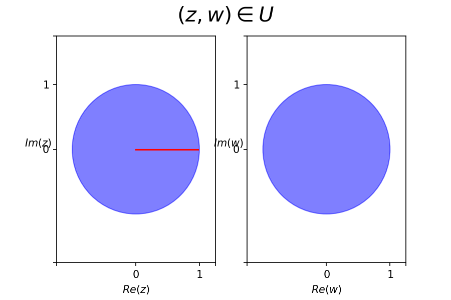
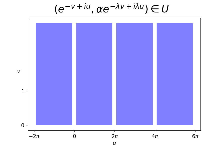
Take the open subset U := { ( z , w ) ∈ 𝔻 2 | z ∉ ℝ ⩾ 0 , w ≠ 0 } assign 𝑈 conditional-set 𝑧 𝑤 superscript 𝔻 2 formulae-sequence 𝑧 subscript ℝ absent 0 𝑤 0 U:=\{(z,w)\in\mathbb{D}^{2}~{}|~{}z\notin\mathbb{R}_{\geqslant 0},w\neq 0\}
Figure 11: Domain U 𝑈 U ( z , w ) 𝑧 𝑤 (z,w) Figure 12: Domain U 𝑈 U ( u , v ) 𝑢 𝑣 (u,v)
Any leaf L α subscript 𝐿 𝛼 L_{\alpha} U 𝑈 U
L α ∩ U = ⋃ k ∈ ℤ L ~ α e 2 k π i λ := ⋃ k ∈ ℤ { ( e − v + i u , α e 2 k π i λ e − λ v + i λ u ) | u ∈ ( 0 , 2 π ) , v > log + | α | λ } . subscript 𝐿 𝛼 𝑈 subscript 𝑘 ℤ subscript ~ 𝐿 𝛼 superscript 𝑒 2 𝑘 𝜋 𝑖 𝜆 assign subscript 𝑘 ℤ conditional-set superscript 𝑒 𝑣 𝑖 𝑢 𝛼 superscript 𝑒 2 𝑘 𝜋 𝑖 𝜆 superscript 𝑒 𝜆 𝑣 𝑖 𝜆 𝑢 formulae-sequence 𝑢 0 2 𝜋 𝑣 superscript 𝛼 𝜆 L_{\alpha}\cap U=\bigcup\limits_{k\in\mathbb{Z}}\tilde{L}_{\alpha\,e^{2k\pi i\lambda}}:=\bigcup\limits_{k\in\mathbb{Z}}\big{\{}(e^{-v+iu},\alpha\,e^{2k\pi i\lambda}\,e^{-\lambda v+i\lambda u})~{}|~{}u\in(0,2\pi),v>\textstyle\frac{\log^{+}|\alpha|}{\lambda}\big{\}}.
Normalizing H α e 2 k π i λ subscript 𝐻 𝛼 superscript 𝑒 2 𝑘 𝜋 𝑖 𝜆 H_{\alpha\,e^{2k\pi i\lambda}} L ~ α e 2 k π i λ subscript ~ 𝐿 𝛼 superscript 𝑒 2 𝑘 𝜋 𝑖 𝜆 \tilde{L}_{\alpha\,e^{2k\pi i\lambda}}
‖ T ‖ U = ∫ α ∈ ℂ ∗ ∫ v > 0 ∫ u = 0 2 π H α ( u + i v ) ‖ ψ α ′ ‖ 2 𝑑 u 𝑑 v 𝑑 μ ( α ) subscript norm 𝑇 𝑈 subscript 𝛼 superscript ℂ subscript 𝑣 0 superscript subscript 𝑢 0 2 𝜋 subscript 𝐻 𝛼 𝑢 𝑖 𝑣 superscript norm superscript subscript 𝜓 𝛼 ′ 2 differential-d 𝑢 differential-d 𝑣 differential-d 𝜇 𝛼 |\!|T|\!|_{U}=\int_{\alpha\in\mathbb{C}^{*}}\int_{v>0}\int_{u=0}^{2\pi}H_{\alpha}(u+iv)|\!|\psi_{\alpha}^{\prime}|\!|^{2}du\,dv\,d\mu(\alpha)
for some positive measure μ 𝜇 \mu ℂ ∗ superscript ℂ \mathbb{C}^{*} ‖ ψ α ′ ‖ 2 superscript norm superscript subscript 𝜓 𝛼 ′ 2 |\!|\psi_{\alpha}^{\prime}|\!|^{2}
| | ψ α ′ | | 2 = { 2 ( e − 2 v + λ 2 | α | 2 e − 2 λ v ) , ( | α | < 1 ) 2 ( | α | − 2 λ e − 2 v + λ 2 e − 2 λ v ) . ( | α | ⩾ 1 ) \displaystyle|\!|\psi_{\alpha}^{\prime}|\!|^{2}=\left\{\begin{aligned} &2(e^{-2v}+\lambda^{2}\,|\alpha|^{2}\,e^{-2\lambda\,v}),&\quad{\scriptstyle{(|\alpha|<1)}}\\
&2(|\alpha|^{-\frac{2}{\lambda}}e^{-2v}+\lambda^{2}\,e^{-2\lambda\,v}).&\quad{\scriptstyle{(|\alpha|\geqslant 1)}}\end{aligned}\right. (5)
Since H 𝐻 H ℍ ℍ \mathbb{H} ℍ ℍ \mathbb{H}
‖ T ‖ U subscript norm 𝑇 𝑈 \displaystyle|\!|T|\!|_{U} = lim ϵ → 0 + ∫ α ∈ ℂ ∗ ∫ v > 0 ∫ u = 0 2 π + ϵ H α ( u + i v ) ‖ ψ α ′ ‖ 2 𝑑 u 𝑑 v 𝑑 μ ( α ) absent subscript → italic-ϵ limit-from 0 subscript 𝛼 superscript ℂ subscript 𝑣 0 superscript subscript 𝑢 0 2 𝜋 italic-ϵ subscript 𝐻 𝛼 𝑢 𝑖 𝑣 superscript norm superscript subscript 𝜓 𝛼 ′ 2 differential-d 𝑢 differential-d 𝑣 differential-d 𝜇 𝛼 \displaystyle=\lim\limits_{\epsilon\rightarrow 0+}\int_{\alpha\in\mathbb{C}^{*}}\int_{v>0}\int_{u=0}^{2\pi+\epsilon}H_{\alpha}(u+iv)|\!|\psi_{\alpha}^{\prime}|\!|^{2}du\,dv\,d\mu(\alpha)
= lim ϵ → 0 + ‖ T ‖ ⋃ k ∈ ℤ L ~ α e 2 k π i λ absent subscript → italic-ϵ limit-from 0 subscript norm 𝑇 subscript 𝑘 ℤ subscript ~ 𝐿 𝛼 superscript 𝑒 2 𝑘 𝜋 𝑖 𝜆 \displaystyle=\lim\limits_{\epsilon\rightarrow 0+}|\!|T|\!|_{\bigcup\limits_{k\in\mathbb{Z}}\tilde{L}_{\alpha\,e^{2k\pi i\lambda}}}
= ‖ T ‖ 𝔻 2 . absent subscript norm 𝑇 superscript 𝔻 2 \displaystyle=|\!|T|\!|_{\mathbb{D}^{2}}.
Thus we can express the mass by a formula independent of the choice of normalization
‖ T ‖ 𝔻 2 = ∫ α ∈ ℂ ∗ ∫ v > 0 ∫ u = 0 2 π H α ( u + i v ) ‖ ψ α ′ ‖ 2 𝑑 u 𝑑 v 𝑑 μ ( α ) . subscript norm 𝑇 superscript 𝔻 2 subscript 𝛼 superscript ℂ subscript 𝑣 0 superscript subscript 𝑢 0 2 𝜋 subscript 𝐻 𝛼 𝑢 𝑖 𝑣 superscript norm superscript subscript 𝜓 𝛼 ′ 2 differential-d 𝑢 differential-d 𝑣 differential-d 𝜇 𝛼 |\!|T|\!|_{\mathbb{D}^{2}}=\int_{\alpha\in\mathbb{C}^{*}}\int_{v>0}\int_{u=0}^{2\pi}H_{\alpha}(u+iv)|\!|\psi_{\alpha}^{\prime}|\!|^{2}du\,dv\,d\mu(\alpha).
Lemma 5.2 .
For each k 0 ∈ ℤ subscript 𝑘 0 ℤ k_{0}\in\mathbb{Z}
‖ T ‖ 𝔻 2 = ∫ α ∈ ℂ ∗ ∫ v > 0 ∫ u = 2 k 0 π 2 k 0 π + 2 π H α ( u + i v ) ‖ ψ α ′ ‖ 2 𝑑 u 𝑑 v 𝑑 μ ( α ) . subscript norm 𝑇 superscript 𝔻 2 subscript 𝛼 superscript ℂ subscript 𝑣 0 superscript subscript 𝑢 2 subscript 𝑘 0 𝜋 2 subscript 𝑘 0 𝜋 2 𝜋 subscript 𝐻 𝛼 𝑢 𝑖 𝑣 superscript norm superscript subscript 𝜓 𝛼 ′ 2 differential-d 𝑢 differential-d 𝑣 differential-d 𝜇 𝛼 |\!|T|\!|_{\mathbb{D}^{2}}=\int_{\alpha\in\mathbb{C}^{*}}\int_{v>0}\int_{u=2k_{0}\pi}^{2k_{0}\pi+2\pi}H_{\alpha}(u+iv)|\!|\psi_{\alpha}^{\prime}|\!|^{2}du\,dv\,d\mu(\alpha).
Proof.
The disjoint union L α ∩ U = ⋃ k ∈ ℤ L ~ α e 2 k π i λ subscript 𝐿 𝛼 𝑈 subscript 𝑘 ℤ subscript ~ 𝐿 𝛼 superscript 𝑒 2 𝑘 𝜋 𝑖 𝜆 L_{\alpha}\cap U=\bigcup\limits_{k\in\mathbb{Z}}\tilde{L}_{\alpha\,e^{2k\pi i\lambda}}
L α ∩ U = ⋃ k ∈ ℤ { ( e − v + i u , α e 2 k π i λ e − λ v + i λ u ) | u ∈ ( 2 k 0 π , 2 k 0 π + 2 π ) , v > log + | α | λ } . subscript 𝐿 𝛼 𝑈 subscript 𝑘 ℤ conditional-set superscript 𝑒 𝑣 𝑖 𝑢 𝛼 superscript 𝑒 2 𝑘 𝜋 𝑖 𝜆 superscript 𝑒 𝜆 𝑣 𝑖 𝜆 𝑢 formulae-sequence 𝑢 2 subscript 𝑘 0 𝜋 2 subscript 𝑘 0 𝜋 2 𝜋 𝑣 superscript 𝛼 𝜆 L_{\alpha}\cap U=\bigcup\limits_{k\in\mathbb{Z}}\big{\{}(e^{-v+iu},\alpha\,e^{2k\pi i\lambda}\,e^{-\lambda v+i\lambda u})~{}|~{}u\in(2k_{0}\pi,2k_{0}\pi+2\pi),v>\textstyle\frac{\log^{+}|\alpha|}{\lambda}\big{\}}.
By the same argument as above one concludes.
∎
5.1 Periodic currents, still a Fourrier series
Periodic currents behave similarly as currents in the rational case λ ∈ ℚ 𝜆 ℚ \lambda\in\mathbb{Q} H α subscript 𝐻 𝛼 H_{\alpha} b ∈ ℤ ⩾ 1 𝑏 subscript ℤ absent 1 b\in\mathbb{Z}_{\geqslant 1} H α ( u + i v ) = H α ( u + 2 π b + i v ) subscript 𝐻 𝛼 𝑢 𝑖 𝑣 subscript 𝐻 𝛼 𝑢 2 𝜋 𝑏 𝑖 𝑣 H_{\alpha}(u+iv)=H_{\alpha}(u+2\pi b+iv) u + i v ∈ ℍ 𝑢 𝑖 𝑣 ℍ u+iv\in\mathbb{H} 2 4.1
According to Lemma 5.2
‖ T ‖ 𝔻 2 subscript norm 𝑇 superscript 𝔻 2 \displaystyle|\!|T|\!|_{\mathbb{D}^{2}} = ∫ α ∈ ℂ ∗ ∫ v > 0 ∫ u = 2 k 0 π 2 k 0 π + 2 π H α ( u + i v ) ‖ ψ α ′ ‖ 2 𝑑 u ∧ d v d μ ( α ) , absent subscript 𝛼 superscript ℂ subscript 𝑣 0 superscript subscript 𝑢 2 subscript 𝑘 0 𝜋 2 subscript 𝑘 0 𝜋 2 𝜋 subscript 𝐻 𝛼 𝑢 𝑖 𝑣 superscript norm superscript subscript 𝜓 𝛼 ′ 2 differential-d 𝑢 𝑑 𝑣 𝑑 𝜇 𝛼 \displaystyle=\int_{\alpha\in\mathbb{C}^{*}}\int_{v>0}\int_{u=2k_{0}\pi}^{2k_{0}\pi+2\pi}H_{\alpha}(u+iv)|\!|\psi_{\alpha}^{\prime}|\!|^{2}\,du\wedge dv\,d\mu(\alpha),
for any k 0 ∈ ℤ subscript 𝑘 0 ℤ k_{0}\in\mathbb{Z} k 0 = 0 , 1 , … , b − 1 subscript 𝑘 0 0 1 … 𝑏 1
k_{0}=0,1,\dots,b-1
b ‖ T ‖ 𝔻 2 𝑏 subscript norm 𝑇 superscript 𝔻 2 \displaystyle b|\!|T|\!|_{\mathbb{D}^{2}} = ∫ α ∈ ℂ ∗ ∫ v > 0 ∫ u = 0 2 π b H α ( u + i v ) ‖ ψ α ′ ‖ 2 𝑑 u ∧ d v d μ ( α ) , absent subscript 𝛼 superscript ℂ subscript 𝑣 0 superscript subscript 𝑢 0 2 𝜋 𝑏 subscript 𝐻 𝛼 𝑢 𝑖 𝑣 superscript norm superscript subscript 𝜓 𝛼 ′ 2 differential-d 𝑢 𝑑 𝑣 𝑑 𝜇 𝛼 \displaystyle=\int_{\alpha\in\mathbb{C}^{*}}\int_{v>0}\int_{u=0}^{2\pi b}H_{\alpha}(u+iv)|\!|\psi_{\alpha}^{\prime}|\!|^{2}\,du\wedge dv\,d\mu(\alpha),
‖ T ‖ 𝔻 2 subscript norm 𝑇 superscript 𝔻 2 \displaystyle|\!|T|\!|_{\mathbb{D}^{2}} = 1 b ∫ α ∈ ℂ ∗ ∫ v > 0 ∫ u = 0 2 π b H α ( u + i v ) ‖ ψ α ′ ‖ 2 𝑑 u ∧ d v d μ ( α ) , absent 1 𝑏 subscript 𝛼 superscript ℂ subscript 𝑣 0 superscript subscript 𝑢 0 2 𝜋 𝑏 subscript 𝐻 𝛼 𝑢 𝑖 𝑣 superscript norm superscript subscript 𝜓 𝛼 ′ 2 differential-d 𝑢 𝑑 𝑣 𝑑 𝜇 𝛼 \displaystyle=\frac{1}{b}\int_{\alpha\in\mathbb{C}^{*}}\int_{v>0}\int_{u=0}^{2\pi b}H_{\alpha}(u+iv)|\!|\psi_{\alpha}^{\prime}|\!|^{2}\,du\wedge dv\,d\mu(\alpha),
= 1 b { ∫ | α | < 1 ∫ v > 0 ∫ u = 0 2 π b H α ( u + i v ) 2 ( e − 2 v + λ 2 | α | 2 e − 2 λ v ) d u ∧ d v d μ ( α ) \displaystyle=\frac{1}{b}\Big{\{}\int_{|\alpha|<1}\int_{v>0}\int_{u=0}^{2\pi b}H_{\alpha}(u+iv)\,2(e^{-2v}+\lambda^{2}\,|\alpha|^{2}\,e^{-2\lambda\,v})\,du\wedge dv\,d\mu(\alpha)
+ ∫ | α | ⩾ 1 ∫ v > 0 ∫ u = 0 2 π b H α ( u + i v ) 2 ( | α | − 2 λ e − 2 v + λ 2 e − 2 λ v ) d u ∧ d v d μ ( α ) } , \displaystyle\ \ \ \ \ \ \ +\int_{|\alpha|\geqslant 1}\int_{v>0}\int_{u=0}^{2\pi b}H_{\alpha}(u+iv)\,2(|\alpha|^{-\frac{2}{\lambda}}\,e^{-2v}+\lambda^{2}\,e^{-2\lambda\,v})\,du\wedge dv\,d\mu(\alpha)\Big{\}},
= 2 π b b { ∫ | α | < 1 ∫ v > 0 ( a 0 ( α ) + b 0 ( α ) v ) 2 ( e − 2 v + λ 2 | α | 2 e − 2 λ v ) d v d μ ( α ) \displaystyle=\frac{2\pi b}{b}\Big{\{}\int_{|\alpha|<1}\int_{v>0}\big{(}a_{0}(\alpha)+b_{0}(\alpha)v\big{)}\,2(e^{-2v}+\lambda^{2}\,|\alpha|^{2}\,e^{-2\lambda\,v})\,dv\,d\mu(\alpha)
+ ∫ | α | ⩾ 1 ∫ v > 0 ( a 0 ( α ) + b 0 ( α ) v ) 2 ( | α | − 2 λ e − 2 v + λ 2 e − 2 λ v ) d v d μ ( α ) } , \displaystyle\ \ \ \ \ \ \ +\int_{|\alpha|\geqslant 1}\int_{v>0}\big{(}a_{0}(\alpha)+b_{0}(\alpha)v\big{)}\,2(|\alpha|^{-\frac{2}{\lambda}}\,e^{-2v}+\lambda^{2}\,e^{-2\lambda\,v})\,dv\,d\mu(\alpha)\Big{\}},
= 2 π { ∫ | α | < 1 a 0 ( α ) ( 1 + | α | 2 λ ) d μ ( α ) + ∫ | α | ⩾ 1 a 0 ( α ) ( | α | − 2 λ + λ ) d μ ( α ) \displaystyle=2\pi\,\Big{\{}\int_{|\alpha|<1}a_{0}(\alpha)\,(1+|\alpha|^{2}\,\lambda)d\mu(\alpha)+\int_{|\alpha|\geqslant 1}a_{0}(\alpha)\,(|\alpha|^{-\frac{2}{\lambda}}+\lambda)d\mu(\alpha)
+ ∫ | α | < 1 b 0 ( α ) ( t 1 2 + 1 2 | α | 2 ) d μ ( α ) + ∫ | α | < 1 b 0 ( α ) ( 1 2 + 1 2 | α | − 2 λ ) d μ ( α ) } \displaystyle\ \ \ \ \ \ +\int_{|\alpha|<1}b_{0}(\alpha)\,\big{(}t\frac{1}{2}+\tfrac{1}{2}|\alpha|^{2}\big{)}d\mu(\alpha)+\int_{|\alpha|<1}b_{0}(\alpha)\,\big{(}\tfrac{1}{2}+\tfrac{1}{2}|\alpha|^{-\frac{2}{\lambda}}\big{)}d\mu(\alpha)\Big{\}}
≈ ∫ α ∈ ℂ ∗ a 0 ( α ) 𝑑 μ ( α ) + ∫ α ∈ ℂ ∗ b 0 ( α ) 𝑑 μ ( α ) , absent subscript 𝛼 superscript ℂ subscript 𝑎 0 𝛼 differential-d 𝜇 𝛼 subscript 𝛼 superscript ℂ subscript 𝑏 0 𝛼 differential-d 𝜇 𝛼 \displaystyle\approx\int_{\alpha\in\mathbb{C}^{*}}a_{0}(\alpha)\,d\mu(\alpha)+\int_{\alpha\in\mathbb{C}^{*}}b_{0}(\alpha)\,d\mu(\alpha),
which is the same expression as in the case λ ∈ ℚ > 0 𝜆 subscript ℚ absent 0 \lambda\in\mathbb{Q}_{>0}
Next, the Lelong number is calculated as
ℒ ( T , 0 ) ℒ 𝑇 0 \displaystyle\mathscr{L}(T,0) = lim r → 0 + 1 r 2 ‖ T ‖ r 𝔻 2 absent subscript → 𝑟 limit-from 0 1 superscript 𝑟 2 subscript norm 𝑇 𝑟 superscript 𝔻 2 \displaystyle=\lim\limits_{r\rightarrow 0+}\frac{1}{r^{2}}|\!|T|\!|_{r\mathbb{D}^{2}}
= lim r → 0 + 1 r 2 2 π { ∫ | α | < r 1 − λ ∫ v > − log r ( a 0 ( α ) + b 0 ( α ) v ) 2 ( e − 2 v + λ 2 | α | 2 e − 2 λ v ) d v d μ ( α ) \displaystyle=\lim\limits_{r\rightarrow 0+}\frac{1}{r^{2}}2\pi\,\Big{\{}\int_{|\alpha|<r^{1-\lambda}}\int_{v>-\log r}\big{(}a_{0}(\alpha)+b_{0}(\alpha)v\big{)}\,2\,(e^{-2v}+\lambda^{2}\,|\alpha|^{2}\,e^{-2\lambda\,v})\,dv\,d\mu(\alpha)
+ ∫ r 1 − λ ⩽ | α | < 1 ∫ v > log | α | − log r λ ( a 0 ( α ) + b 0 ( α ) v ) 2 ( e − 2 v + λ 2 | α | 2 e − 2 λ v ) d v d μ ( α ) } \displaystyle\ \ \ \ \ \ \ \ \ \ \ \ \ \ \ \ +\,\int_{r^{1-\lambda}\leqslant|\alpha|<1}\int_{v>\frac{\log|\alpha|-\log r}{\lambda}}\big{(}a_{0}(\alpha)+b_{0}(\alpha)v\big{)}\,2\,(e^{-2v}+\lambda^{2}\,|\alpha|^{2}\,e^{-2\lambda\,v})\,dv\,d\mu(\alpha)\Big{\}}
+ ∫ | α | ⩾ 1 ∫ v > − log r λ ( a 0 ( α ) + b 0 ( α ) v ) 2 ( | α | − 2 λ e − 2 v + λ 2 e − 2 λ v ) d v d μ ( α ) } \displaystyle\ \ \ \ \ \ \ \ \ \ \ \ \ \ \ \ +\,\int_{|\alpha|\geqslant 1}\int_{v>\frac{-\log r}{\lambda}}\big{(}a_{0}(\alpha)+b_{0}(\alpha)v\big{)}\,2\,(|\alpha|^{-\frac{2}{\lambda}}e^{-2v}+\lambda^{2}\,e^{-2\lambda\,v})\,dv\,d\mu(\alpha)\Big{\}}
= lim r → 0 + 2 π { ∫ | α | < r 1 − λ a 0 ( α ) ( 1 + λ | α | 2 r 2 λ − 2 ) d μ ( α ) \displaystyle=\lim\limits_{r\rightarrow 0+}2\pi\,\Big{\{}\int_{|\alpha|<r^{1-\lambda}}a_{0}(\alpha)\,(1+\lambda\,|\alpha|^{2}\,r^{2\lambda-2})\,d\mu(\alpha)
+ ∫ | α | ⩾ r 1 − λ a 0 ( α ) ( | α | − 2 λ r 2 λ − 2 + λ ) 𝑑 μ ( α ) subscript 𝛼 superscript 𝑟 1 𝜆 subscript 𝑎 0 𝛼 superscript 𝛼 2 𝜆 superscript 𝑟 2 𝜆 2 𝜆 differential-d 𝜇 𝛼 \displaystyle\ \ \ \ \ \ \ \ \ \ \ \ \ +\int_{|\alpha|\geqslant r^{1-\lambda}}a_{0}(\alpha)\,(|\alpha|^{-\frac{2}{\lambda}}\,r^{\frac{2}{\lambda}-2}+\lambda)\,d\mu(\alpha)
+ ∫ | α | < r 1 − λ b 0 ( α ) ( 1 2 + 1 2 | α | 2 r 2 λ − 2 − log r − λ | α | 2 r 2 λ − 2 log r ) 𝑑 μ ( α ) subscript 𝛼 superscript 𝑟 1 𝜆 subscript 𝑏 0 𝛼 1 2 1 2 superscript 𝛼 2 superscript 𝑟 2 𝜆 2 𝑟 𝜆 superscript 𝛼 2 superscript 𝑟 2 𝜆 2 𝑟 differential-d 𝜇 𝛼 \displaystyle\ \ \ \ \ \ \ \ \ \ \ \ \ +\int_{|\alpha|<r^{1-\lambda}}b_{0}(\alpha)\,\big{(}\tfrac{1}{2}+\tfrac{1}{2}|\alpha|^{2}\,r^{2\lambda-2}-\log r-\lambda\,|\alpha|^{2}\,r^{2\lambda-2}\,\log r\big{)}\,d\mu(\alpha)
+ ∫ r 1 − λ ⩽ | α | < 1 b 0 ( α ) ( 1 2 + 1 2 | α | − 2 λ r 2 λ − 2 − log r − λ − 1 | α | − 2 λ r 2 λ − 2 log r \displaystyle\ \ \ \ \ \ \ \ \ \ \ \ \ +\int_{r^{1-\lambda}\leqslant|\alpha|<1}b_{0}(\alpha)\,\big{(}\tfrac{1}{2}+\tfrac{1}{2}|\alpha|^{-\frac{2}{\lambda}}\,r^{\frac{2}{\lambda}-2}-\log r-\lambda^{-1}\,|\alpha|^{-\frac{2}{\lambda}}\,r^{2\lambda-2}\log r
+ log | α | + λ − 1 | α | − 2 λ log | α | r 2 λ − 2 ) d μ ( α ) \displaystyle\ \ \ \ \ \ \ \ \ \ \ \ \ \ \ \ \ \ \ \ \ \ \ \ \ \ \ \ \ \ \ \ \ \ \ \ \ \ \ +\log|\alpha|+\lambda^{-1}\,|\alpha|^{-\frac{2}{\lambda}}\,\log|\alpha|\,r^{2\lambda-2}\big{)}\,d\mu(\alpha)
+ ∫ | α | ⩾ 1 b 0 ( α ) ( 1 2 + 1 2 | α | − 2 λ r 2 λ − 2 − log r − λ − 1 | α | − 2 λ r 2 λ − 2 log r ) d μ ( α ) } . \displaystyle\ \ \ \ \ \ \ \ \ \ \ \ \ +\int_{|\alpha|\geqslant 1}b_{0}(\alpha)\,\big{(}\tfrac{1}{2}+\tfrac{1}{2}|\alpha|^{-\frac{2}{\lambda}}\,r^{\frac{2}{\lambda}-2}-\log r-\lambda^{-1}\,|\alpha|^{-\frac{2}{\lambda}}\,r^{2\lambda-2}\log r\big{)}\,d\mu(\alpha)\Big{\}}.
exactly the same expression as in the case λ = 1 𝜆 1 \lambda=1 4.2 b 0 ( α ) = 0 subscript 𝑏 0 𝛼 0 b_{0}(\alpha)=0 μ 𝜇 \mu α ∈ ℂ ∗ 𝛼 superscript ℂ \alpha\in\mathbb{C}^{*}
ℒ ( T , 0 ) ≈ ∫ α ∈ ℂ ∗ a 0 ( α ) 𝑑 μ ( α ) ≈ ‖ T ‖ 𝔻 2 . ℒ 𝑇 0 subscript 𝛼 superscript ℂ subscript 𝑎 0 𝛼 differential-d 𝜇 𝛼 subscript norm 𝑇 superscript 𝔻 2 \mathscr{L}(T,0)\approx\int_{\alpha\in\mathbb{C}^{*}}a_{0}(\alpha)\,d\mu(\alpha)\approx|\!|T|\!|_{\mathbb{D}^{2}}.
The Lelong number is strictly positive, the same as in the case λ ∈ ℚ ∪ ( 0 , 1 ) 𝜆 ℚ 0 1 \lambda\in\mathbb{Q}\cup(0,1)
5.2 Non-periodic current
For periodic currents, one takes an average among b 𝑏 b 4.1 4.1 k 0 ∈ ℤ subscript 𝑘 0 ℤ k_{0}\in\mathbb{Z}
The Lelong number is expressed by
ℒ ( T , 0 ) ℒ 𝑇 0 \displaystyle\mathscr{L}(T,0) = lim r → 0 + 1 r 2 { ∫ | α | < r 1 − λ ∫ v > − log r ∫ u = 0 2 π H α ( u + i v ) | | ψ α ′ | | 2 d u d v d μ ( α ) \displaystyle=\lim\limits_{r\rightarrow 0+}\frac{1}{r^{2}}\Big{\{}\int_{|\alpha|<r^{1-\lambda}}\int_{v>-\log r}\int_{u=0}^{2\pi}H_{\alpha}(u+iv)|\!|\psi_{\alpha}^{\prime}|\!|^{2}du\,dv\,d\mu(\alpha)
+ ∫ r 1 − λ ⩽ | α | < 1 ∫ v > log | α | − log r λ ∫ u = 0 2 π H α ( u + i v ) ‖ ψ α ′ ‖ 2 𝑑 u 𝑑 v 𝑑 μ ( α ) subscript superscript 𝑟 1 𝜆 𝛼 1 subscript 𝑣 𝛼 𝑟 𝜆 superscript subscript 𝑢 0 2 𝜋 subscript 𝐻 𝛼 𝑢 𝑖 𝑣 superscript norm superscript subscript 𝜓 𝛼 ′ 2 differential-d 𝑢 differential-d 𝑣 differential-d 𝜇 𝛼 \displaystyle\ \ \ \ \ \ \ \ \ \ \ \ \ +\int_{r^{1-\lambda}\leqslant|\alpha|<1}\int_{v>\frac{\log|\alpha|-\log r}{\lambda}}\int_{u=0}^{2\pi}H_{\alpha}(u+iv)|\!|\psi_{\alpha}^{\prime}|\!|^{2}du\,dv\,d\mu(\alpha)
+ ∫ | α | ⩾ 1 | ∫ v > − log r λ ∫ u = 0 2 π H α ( u + i v ) | | ψ α ′ | | 2 d u d v d μ ( α ) } \displaystyle\ \ \ \ \ \ \ \ \ \ \ \ \ +\int_{|\alpha|\geqslant 1|}\int_{v>\frac{-\log r}{\lambda}}\int_{u=0}^{2\pi}H_{\alpha}(u+iv)|\!|\psi_{\alpha}^{\prime}|\!|^{2}du\,dv\,d\mu(\alpha)\Big{\}}
Recall the Poisson integral formula after multiplying a nonzero constant
H α ( u + i v ) = 1 π ∫ y ∈ ℝ H α ( y ) v v 2 + ( y − u ) 2 𝑑 y + C α v . subscript 𝐻 𝛼 𝑢 𝑖 𝑣 1 𝜋 subscript 𝑦 ℝ subscript 𝐻 𝛼 𝑦 𝑣 superscript 𝑣 2 superscript 𝑦 𝑢 2 differential-d 𝑦 subscript 𝐶 𝛼 𝑣 H_{\alpha}(u+iv)=\frac{1}{\pi}\,\int_{y\in\mathbb{R}}H_{\alpha}(y)\,\frac{v}{v^{2}+(y-u)^{2}}\,dy+{C}_{\alpha}\,v.
Using the same argument as in Lemma 4.2 C α = 0 subscript 𝐶 𝛼 0 {C}_{\alpha}=0 α ∈ ℂ ∗ 𝛼 superscript ℂ \alpha\in\mathbb{C}^{*}
Lemma 5.3 .
For any v ⩾ 1 λ > 1 𝑣 1 𝜆 1 v\geqslant\frac{1}{\lambda}>1 u ∈ ℝ 𝑢 ℝ u\in\mathbb{R}
∂ ∂ v ( − 1 2 v v 2 + ( u − y ) 2 e − 2 v ) v v 2 + ( u − y ) 2 e − 2 v ∈ ( 1 2 , 2 ) , 𝑣 1 2 𝑣 superscript 𝑣 2 superscript 𝑢 𝑦 2 superscript 𝑒 2 𝑣 𝑣 superscript 𝑣 2 superscript 𝑢 𝑦 2 superscript 𝑒 2 𝑣 1 2 2 \displaystyle\frac{\frac{\partial}{\partial v}\Big{(}-\frac{1}{2}\frac{v}{v^{2}+(u-y)^{2}}e^{-2v}\Big{)}}{\frac{v}{v^{2}+(u-y)^{2}}e^{-2v}}\in\Big{(}\frac{1}{2},2\Big{)},
∂ ∂ v ( − 1 2 λ v v 2 + ( u − y ) 2 e − 2 λ v ) v v 2 + ( u − y ) 2 e − 2 λ v ∈ ( 1 2 , 2 ) . 𝑣 1 2 𝜆 𝑣 superscript 𝑣 2 superscript 𝑢 𝑦 2 superscript 𝑒 2 𝜆 𝑣 𝑣 superscript 𝑣 2 superscript 𝑢 𝑦 2 superscript 𝑒 2 𝜆 𝑣 1 2 2 \displaystyle\frac{\frac{\partial}{\partial v}\Big{(}-\frac{1}{2\lambda}\frac{v}{v^{2}+(u-y)^{2}}e^{-2\lambda v}\Big{)}}{\frac{v}{v^{2}+(u-y)^{2}}e^{-2\lambda v}}\in\Big{(}\frac{1}{2},2\Big{)}.
Proof.
This can be calculated directly,
∂ ∂ v ( − 1 2 v v 2 + ( u − y ) 2 e − 2 v ) 𝑣 1 2 𝑣 superscript 𝑣 2 superscript 𝑢 𝑦 2 superscript 𝑒 2 𝑣 \displaystyle\frac{\partial}{\partial v}\Big{(}-\frac{1}{2}\frac{v}{v^{2}+(u-y)^{2}}e^{-2v}\Big{)} = ( v v 2 + ( u − y ) 2 + ( − 1 2 ) 1 v 2 + ( u − y ) 2 + ( − 1 2 ) v ( − 2 v ) ( v 2 + ( u − y ) 2 ) 2 ) e − 2 v absent 𝑣 superscript 𝑣 2 superscript 𝑢 𝑦 2 1 2 1 superscript 𝑣 2 superscript 𝑢 𝑦 2 1 2 𝑣 2 𝑣 superscript superscript 𝑣 2 superscript 𝑢 𝑦 2 2 superscript 𝑒 2 𝑣 \displaystyle=\Big{(}\frac{v}{v^{2}+(u-y)^{2}}+\big{(}-\frac{1}{2}\big{)}\frac{1}{v^{2}+(u-y)^{2}}+\big{(}-\frac{1}{2}\big{)}\frac{v(-2v)}{\big{(}v^{2}+(u-y)^{2}\big{)}^{2}}\Big{)}\,e^{-2v}
∂ ∂ v ( − 1 2 v v 2 + ( u − y ) 2 e − 2 v ) v v 2 + ( u − y ) 2 e − 2 v 𝑣 1 2 𝑣 superscript 𝑣 2 superscript 𝑢 𝑦 2 superscript 𝑒 2 𝑣 𝑣 superscript 𝑣 2 superscript 𝑢 𝑦 2 superscript 𝑒 2 𝑣 \displaystyle\frac{\frac{\partial}{\partial v}\Big{(}-\frac{1}{2}\frac{v}{v^{2}+(u-y)^{2}}e^{-2v}\Big{)}}{\frac{v}{v^{2}+(u-y)^{2}}e^{-2v}} = 1 + ( − 1 2 1 v ) + v v 2 + ( u − y ) 2 absent 1 1 2 1 𝑣 𝑣 superscript 𝑣 2 superscript 𝑢 𝑦 2 \displaystyle=1+\big{(}-\frac{1}{2}\frac{1}{v}\big{)}+\frac{v}{v^{2}+(u-y)^{2}}
∈ ( 1 − 1 2 v , 1 + 1 v ) ⊆ ( 1 2 , 2 ) , ( v > 1 ) , formulae-sequence absent 1 1 2 𝑣 1 1 𝑣 1 2 2 𝑣 1 \displaystyle\in\Big{(}1-\frac{1}{2v},1+\frac{1}{v}\Big{)}\subseteq\Big{(}\frac{1}{2},2\Big{)},\quad{\scriptstyle{(v>1)}},
∂ ∂ v ( − 1 2 λ v v 2 + ( u − y ) 2 e − 2 λ v ) 𝑣 1 2 𝜆 𝑣 superscript 𝑣 2 superscript 𝑢 𝑦 2 superscript 𝑒 2 𝜆 𝑣 \displaystyle\frac{\partial}{\partial v}\Big{(}-\frac{1}{2\lambda}\frac{v}{v^{2}+(u-y)^{2}}e^{-2\lambda v}\Big{)} = ( v v 2 + ( u − y ) 2 + ( − 1 2 λ ) 1 v 2 + ( u − y ) 2 + ( − 1 2 λ ) v ( − 2 v ) ( v 2 + ( u − y ) 2 ) 2 ) e − 2 λ v absent 𝑣 superscript 𝑣 2 superscript 𝑢 𝑦 2 1 2 𝜆 1 superscript 𝑣 2 superscript 𝑢 𝑦 2 1 2 𝜆 𝑣 2 𝑣 superscript superscript 𝑣 2 superscript 𝑢 𝑦 2 2 superscript 𝑒 2 𝜆 𝑣 \displaystyle=\Big{(}\frac{v}{v^{2}+(u-y)^{2}}+\big{(}-\frac{1}{2\lambda}\big{)}\frac{1}{v^{2}+(u-y)^{2}}+\big{(}-\frac{1}{2\lambda}\big{)}\frac{v(-2v)}{\big{(}v^{2}+(u-y)^{2}\big{)}^{2}}\Big{)}\,e^{-2\lambda v}
∂ ∂ v ( − 1 2 λ v v 2 + ( u − y ) 2 e − 2 λ v ) v v 2 + ( u − y ) 2 e − 2 λ v 𝑣 1 2 𝜆 𝑣 superscript 𝑣 2 superscript 𝑢 𝑦 2 superscript 𝑒 2 𝜆 𝑣 𝑣 superscript 𝑣 2 superscript 𝑢 𝑦 2 superscript 𝑒 2 𝜆 𝑣 \displaystyle\frac{\frac{\partial}{\partial v}\Big{(}-\frac{1}{2\lambda}\frac{v}{v^{2}+(u-y)^{2}}e^{-2\lambda v}\Big{)}}{\frac{v}{v^{2}+(u-y)^{2}}e^{-2\lambda v}} = 1 + ( − 1 2 λ 1 v ) + 1 λ v v 2 + ( u − y ) 2 absent 1 1 2 𝜆 1 𝑣 1 𝜆 𝑣 superscript 𝑣 2 superscript 𝑢 𝑦 2 \displaystyle=1+\big{(}-\frac{1}{2\lambda}\frac{1}{v}\big{)}+\frac{1}{\lambda}\frac{v}{v^{2}+(u-y)^{2}}
∈ ( 1 − 1 2 λ v , 1 + 1 λ v ) ⊆ ( 1 2 , 2 ) , ( v ⩾ 1 λ ) . ∎ formulae-sequence absent 1 1 2 𝜆 𝑣 1 1 𝜆 𝑣 1 2 2 𝑣 1 𝜆 \displaystyle\in\Big{(}1-\frac{1}{2\lambda v},1+\frac{1}{\lambda v}\Big{)}\subseteq\Big{(}\frac{1}{2},2\Big{)},\quad{\scriptstyle{(v\geqslant\frac{1}{\lambda})}}.\qed
Corollary 5.4 .
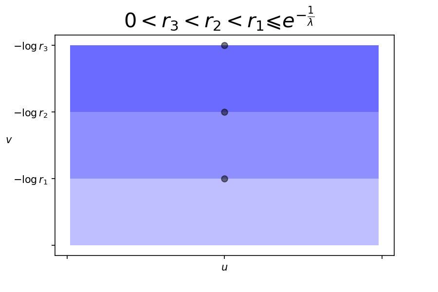
For any r 𝑟 r 0 < r ⩽ e − 1 λ 0 𝑟 superscript 𝑒 1 𝜆 0<r\leqslant e^{-\frac{1}{\lambda}}
1 r 2 ∫ v > − log r H α ( u + i v ) ‖ ψ α ′ ‖ 2 𝑑 v 1 superscript 𝑟 2 subscript 𝑣 𝑟 subscript 𝐻 𝛼 𝑢 𝑖 𝑣 superscript norm superscript subscript 𝜓 𝛼 ′ 2 differential-d 𝑣 \displaystyle\frac{1}{r^{2}}\int_{v>-\log r}H_{\alpha}(u+iv)|\!|\psi_{\alpha}^{\prime}|\!|^{2}dv ≈ H α ( u + ( − log r ) i ) , ( 0 < | α | < r 1 − λ ) absent subscript 𝐻 𝛼 𝑢 𝑟 𝑖 0 𝛼 superscript 𝑟 1 𝜆
\displaystyle\approx H_{\alpha}\big{(}u+(-\log r)i\big{)},\quad{\scriptstyle{(0<|\alpha|<r^{1-\lambda})}}
1 r 2 ∫ v > log | α | − log r λ H α ( u + i v ) ‖ ψ α ′ ‖ 2 𝑑 v 1 superscript 𝑟 2 subscript 𝑣 𝛼 𝑟 𝜆 subscript 𝐻 𝛼 𝑢 𝑖 𝑣 superscript norm superscript subscript 𝜓 𝛼 ′ 2 differential-d 𝑣 \displaystyle\frac{1}{r^{2}}\int_{v>\frac{\log|\alpha|-\log r}{\lambda}}H_{\alpha}(u+iv)|\!|\psi_{\alpha}^{\prime}|\!|^{2}dv ≈ H α ( u + ( log | α | − log r λ ) i ) , ( 0 < | α | < r 1 − λ ) absent subscript 𝐻 𝛼 𝑢 𝛼 𝑟 𝜆 𝑖 0 𝛼 superscript 𝑟 1 𝜆
\displaystyle\approx H_{\alpha}\big{(}u+(\textstyle\frac{\log|\alpha|-\log r}{\lambda})i\big{)},\quad{\scriptstyle{(0<|\alpha|<r^{1-\lambda})}}
1 r 2 ∫ v > log | α | − log r λ H α ( u + i v ) ‖ ψ α ′ ‖ 2 𝑑 v 1 superscript 𝑟 2 subscript 𝑣 𝛼 𝑟 𝜆 subscript 𝐻 𝛼 𝑢 𝑖 𝑣 superscript norm superscript subscript 𝜓 𝛼 ′ 2 differential-d 𝑣 \displaystyle\frac{1}{r^{2}}\int_{v>\frac{\log|\alpha|-\log r}{\lambda}}H_{\alpha}(u+iv)|\!|\psi_{\alpha}^{\prime}|\!|^{2}dv ≈ H α ( u + ( − log r λ ) i ) , ( 0 < | α | < r 1 − λ ) absent subscript 𝐻 𝛼 𝑢 𝑟 𝜆 𝑖 0 𝛼 superscript 𝑟 1 𝜆
\displaystyle\approx H_{\alpha}\big{(}u+(\textstyle\frac{-\log r}{\lambda})i\big{)},\quad{\scriptstyle{(0<|\alpha|<r^{1-\lambda})}}
Figure 13: 1 r 2 1 superscript 𝑟 2 \frac{1}{r^{2}} v > − log r 𝑣 𝑟 v>-\log r ≈ \approx v = log r 𝑣 𝑟 v=\log r
Proof.
When 0 < r ⩽ e − 1 λ 0 𝑟 superscript 𝑒 1 𝜆 0<r\leqslant e^{-\frac{1}{\lambda}} − log r ⩾ 1 λ 𝑟 1 𝜆 -\log r\geqslant\frac{1}{\lambda} 5.3
∫ v > − log r H α ( u + i v ) ‖ ψ α ′ ‖ 2 𝑑 v subscript 𝑣 𝑟 subscript 𝐻 𝛼 𝑢 𝑖 𝑣 superscript norm superscript subscript 𝜓 𝛼 ′ 2 differential-d 𝑣 \displaystyle\int_{v>-\log r}H_{\alpha}(u+iv)|\!|\psi_{\alpha}^{\prime}|\!|^{2}dv = 1 π ∫ v > − log r ∫ y ∈ ℝ H α ( y ) v v 2 + ( u − y ) 2 2 ( e − 2 v + λ 2 | α | 2 e − 2 λ v ) 𝑑 y 𝑑 v absent 1 𝜋 subscript 𝑣 𝑟 subscript 𝑦 ℝ subscript 𝐻 𝛼 𝑦 𝑣 superscript 𝑣 2 superscript 𝑢 𝑦 2 2 superscript 𝑒 2 𝑣 superscript 𝜆 2 superscript 𝛼 2 superscript 𝑒 2 𝜆 𝑣 differential-d 𝑦 differential-d 𝑣 \displaystyle=\frac{1}{\pi}\int_{v>-\log r}\int_{y\in\mathbb{R}}H_{\alpha}(y)\frac{v}{v^{2}+(u-y)^{2}}2\,(e^{-2v}+\lambda^{2}\,|\alpha|^{2}\,e^{-2\lambda v})dy\,dv
≈ 1 π ∫ y ∈ ℝ H α ( y ) { ∫ v > − log r ∂ ∂ v ( v v 2 + ( u − y ) 2 ( − e − 2 v − λ | α | 2 e − 2 λ v ) ) 𝑑 v } 𝑑 y absent 1 𝜋 subscript 𝑦 ℝ subscript 𝐻 𝛼 𝑦 subscript 𝑣 𝑟 𝑣 𝑣 superscript 𝑣 2 superscript 𝑢 𝑦 2 superscript 𝑒 2 𝑣 𝜆 superscript 𝛼 2 superscript 𝑒 2 𝜆 𝑣 differential-d 𝑣 differential-d 𝑦 \displaystyle\approx\frac{1}{\pi}\int_{y\in\mathbb{R}}H_{\alpha}(y)\Big{\{}\int_{v>-\log r}\frac{\partial}{\partial v}\Big{(}\frac{v}{v^{2}+(u-y)^{2}}\big{(}-e^{-2v}-\lambda\,|\alpha|^{2}\,e^{-2\lambda v}\big{)}\Big{)}dv\Big{\}}\,dy
= 1 π ∫ y ∈ ℝ H α ( y ) − log r ( − log r ) 2 + ( u − y ) 2 ( r 2 + λ | α | 2 r 2 λ ) 𝑑 y absent 1 𝜋 subscript 𝑦 ℝ subscript 𝐻 𝛼 𝑦 𝑟 superscript 𝑟 2 superscript 𝑢 𝑦 2 superscript 𝑟 2 𝜆 superscript 𝛼 2 superscript 𝑟 2 𝜆 differential-d 𝑦 \displaystyle=\frac{1}{\pi}\int_{y\in\mathbb{R}}H_{\alpha}(y)\frac{-\log r}{(-\log r)^{2}+(u-y)^{2}}\big{(}r^{2}+\lambda\,|\alpha|^{2}\,r^{2\lambda}\big{)}dy
= H α ( u + ( − log r ) i ) ( r 2 + λ | α | 2 r 2 λ ) absent subscript 𝐻 𝛼 𝑢 𝑟 𝑖 superscript 𝑟 2 𝜆 superscript 𝛼 2 superscript 𝑟 2 𝜆 \displaystyle=H_{\alpha}\big{(}u+(-\log r)i\big{)}\big{(}r^{2}+\lambda\,|\alpha|^{2}\,r^{2\lambda}\big{)}
≈ r 2 H α ( u + ( − log r ) i ) . absent superscript 𝑟 2 subscript 𝐻 𝛼 𝑢 𝑟 𝑖 \displaystyle\approx r^{2}\,H_{\alpha}\big{(}u+(-\log r)i\big{)}.
For the same reason when r 1 − λ ⩽ | α | < 1 superscript 𝑟 1 𝜆 𝛼 1 r^{1-\lambda}\leqslant|\alpha|<1 log | α | − log r λ ⩾ − log r ⩾ 1 λ 𝛼 𝑟 𝜆 𝑟 1 𝜆 \frac{\log|\alpha|-\log r}{\lambda}\geqslant-\log r\geqslant\frac{1}{\lambda}
∫ v > log | α | − log r λ H α ( u + i v ) ‖ ψ α ′ ‖ 2 𝑑 v subscript 𝑣 𝛼 𝑟 𝜆 subscript 𝐻 𝛼 𝑢 𝑖 𝑣 superscript norm superscript subscript 𝜓 𝛼 ′ 2 differential-d 𝑣 \displaystyle\int_{v>\frac{\log|\alpha|-\log r}{\lambda}}H_{\alpha}(u+iv)|\!|\psi_{\alpha}^{\prime}|\!|^{2}dv ≈ H α ( u + ( log | α | − log r λ ) i ) ( | α | − 2 λ r 2 λ + λ r 2 ) absent subscript 𝐻 𝛼 𝑢 𝛼 𝑟 𝜆 𝑖 superscript 𝛼 2 𝜆 superscript 𝑟 2 𝜆 𝜆 superscript 𝑟 2 \displaystyle\approx H_{\alpha}\big{(}u+(\textstyle\frac{\log|\alpha|-\log r}{\lambda})i\big{)}\,\big{(}|\alpha|^{-\frac{2}{\lambda}}\,r^{\frac{2}{\lambda}}+\lambda\,r^{2})
≈ r 2 H α ( u + ( log | α | − log r λ ) i ) . absent superscript 𝑟 2 subscript 𝐻 𝛼 𝑢 𝛼 𝑟 𝜆 𝑖 \displaystyle\approx r^{2}\,H_{\alpha}\big{(}u+(\textstyle\frac{\log|\alpha|-\log r}{\lambda})i\big{)}.
Last, when | α | ⩾ 1 𝛼 1 |\alpha|\geqslant 1 − log r λ ⩾ − log r ⩾ 1 λ 𝑟 𝜆 𝑟 1 𝜆 \frac{-\log r}{\lambda}\geqslant-\log r\geqslant\frac{1}{\lambda}
∫ v > − log r λ H α ( u + i v ) ‖ ψ α ′ ‖ 2 𝑑 v subscript 𝑣 𝑟 𝜆 subscript 𝐻 𝛼 𝑢 𝑖 𝑣 superscript norm superscript subscript 𝜓 𝛼 ′ 2 differential-d 𝑣 \displaystyle\int_{v>\frac{-\log r}{\lambda}}H_{\alpha}(u+iv)|\!|\psi_{\alpha}^{\prime}|\!|^{2}dv ≈ H α ( u + ( − log r λ ) i ) ( | α | − 2 λ r 2 λ + λ r 2 ) absent subscript 𝐻 𝛼 𝑢 𝑟 𝜆 𝑖 superscript 𝛼 2 𝜆 superscript 𝑟 2 𝜆 𝜆 superscript 𝑟 2 \displaystyle\approx H_{\alpha}\big{(}u+(\textstyle\frac{-\log r}{\lambda})i\big{)}\,\big{(}|\alpha|^{-\frac{2}{\lambda}}\,r^{\frac{2}{\lambda}}+\lambda\,r^{2})
≈ r 2 H α ( u + ( − log r λ ) i ) . ∎ absent superscript 𝑟 2 subscript 𝐻 𝛼 𝑢 𝑟 𝜆 𝑖 \displaystyle\approx r^{2}\,H_{\alpha}\big{(}u+(\textstyle\frac{-\log r}{\lambda})i\big{)}.\qed
Thus
ℒ ( T , 0 ) ℒ 𝑇 0 \displaystyle\mathscr{L}(T,0) ≈ lim r → 0 + { ∫ | α | < r 1 − λ ∫ u = 0 2 π H α ( u + ( − log r ) i ) d u d μ ( α ) \displaystyle\approx\lim\limits_{r\rightarrow 0+}\Big{\{}\int_{|\alpha|<r^{1-\lambda}}\int_{u=0}^{2\pi}H_{\alpha}\big{(}u+(-\log r)i\big{)}\,du\,d\mu(\alpha)
+ ∫ r 1 − λ ⩽ | α | < 1 ∫ u = 0 2 π H α ( u + ( log | α | − log r λ ) i ) 𝑑 u 𝑑 μ ( α ) subscript superscript 𝑟 1 𝜆 𝛼 1 superscript subscript 𝑢 0 2 𝜋 subscript 𝐻 𝛼 𝑢 𝛼 𝑟 𝜆 𝑖 differential-d 𝑢 differential-d 𝜇 𝛼 \displaystyle\ \ \ \ \ \ \ \ \ \ +\int_{r^{1-\lambda}\leqslant|\alpha|<1}\int_{u=0}^{2\pi}H_{\alpha}\big{(}u+(\textstyle\frac{\log|\alpha|-\log r}{\lambda})i\big{)}\,du\,d\mu(\alpha)
+ ∫ | α | ⩾ 1 ∫ u = 0 2 π H α ( u + ( − log r λ ) i ) d u d μ ( α ) } , \displaystyle\ \ \ \ \ \ \ \ \ \ +\int_{|\alpha|\geqslant 1}\int_{u=0}^{2\pi}H_{\alpha}\big{(}u+(\textstyle\frac{-\log r}{\lambda})i\big{)}\,du\,d\mu(\alpha)\Big{\}},
by the inequalities (3 4
ℒ ( T , 0 ) ℒ 𝑇 0 \displaystyle\mathscr{L}(T,0) ≈ lim v → + ∞ ∫ α ∈ ℂ ∗ ∫ u = 0 2 π H α ( u + i v ) 𝑑 u 𝑑 μ ( α ) absent subscript → 𝑣 subscript 𝛼 superscript ℂ superscript subscript 𝑢 0 2 𝜋 subscript 𝐻 𝛼 𝑢 𝑖 𝑣 differential-d 𝑢 differential-d 𝜇 𝛼 \displaystyle\approx\lim\limits_{v\rightarrow+\infty}\int_{\alpha\in\mathbb{C}^{*}}\int_{u=0}^{2\pi}H_{\alpha}\big{(}u+iv\big{)}\,du\,d\mu(\alpha)
= lim k → + ∞ ∫ α ∈ ℂ ∗ ∫ u = 0 2 π ∫ y ∈ ℝ H α ( y ) 2 k π ( 2 k π ) 2 + ( u − y ) 2 𝑑 y 𝑑 u 𝑑 μ ( α ) , absent subscript → 𝑘 subscript 𝛼 superscript ℂ superscript subscript 𝑢 0 2 𝜋 subscript 𝑦 ℝ subscript 𝐻 𝛼 𝑦 2 𝑘 𝜋 superscript 2 𝑘 𝜋 2 superscript 𝑢 𝑦 2 differential-d 𝑦 differential-d 𝑢 differential-d 𝜇 𝛼 \displaystyle=\lim\limits_{k\rightarrow+\infty}\int_{\alpha\in\mathbb{C}^{*}}\int_{u=0}^{2\pi}\int_{y\in\mathbb{R}}H_{\alpha}(y)\frac{2k\pi}{(2k\pi)^{2}+(u-y)^{2}}\,dy\,du\,d\mu(\alpha),
Fix some k ∈ ℤ 𝑘 ℤ k\in\mathbb{Z} k ⩾ 2 𝑘 2 k\geqslant 2 I N subscript 𝐼 𝑁 I_{N} N ∈ ℤ 𝑁 ℤ N\in\mathbb{Z}
I 0 subscript 𝐼 0 \displaystyle I_{0} = [ − 2 k π + 2 π , 2 k π ) , absent 2 𝑘 𝜋 2 𝜋 2 𝑘 𝜋 \displaystyle=[-2k\pi+2\pi,2k\pi),
I N subscript 𝐼 𝑁 \displaystyle I_{N} = { [ 2 k π N , 2 k π ( N + 1 ) ) , ( N > 0 ) [ 2 k π ( N − 1 ) + 2 π , 2 k π N + 2 π ) , ( N < 0 ) \displaystyle=\left\{\begin{aligned} &\big{[}2k\pi N,2k\pi(N+1)\big{)},&\quad{\scriptstyle{(N>0)}}\\
&\big{[}2k\pi(N-1)+2\pi,2k\pi N+2\pi\big{)},&\quad{\scriptstyle{(N<0)}}\end{aligned}\right.
Thus ℝ = ⋃ N ∈ ℤ I N ℝ subscript 𝑁 ℤ subscript 𝐼 𝑁 \mathbb{R}=\bigcup\limits_{N\in\mathbb{Z}}I_{N}
Lemma 5.5 .
For any u ∈ ( 0 , 2 π ) 𝑢 0 2 𝜋 u\in(0,2\pi)
2 k π ( 2 k π ) 2 + ( u − y ) 2 ⩾ 1 1 + ( N + 1 ) 2 1 2 k π , ( y ∈ I N ) 2 𝑘 𝜋 superscript 2 𝑘 𝜋 2 superscript 𝑢 𝑦 2 1 1 superscript 𝑁 1 2 1 2 𝑘 𝜋 𝑦 subscript 𝐼 𝑁
\frac{2k\pi}{(2k\pi)^{2}+(u-y)^{2}}\geqslant\frac{1}{1+(N+1)^{2}}\frac{1}{2k\pi},\quad{\scriptstyle{(y\in I_{N})}}
Thus
ℒ ( T , 0 ) ℒ 𝑇 0 \displaystyle\mathscr{L}(T,0) ≈ lim k → + ∞ ∑ N ∈ ℤ ∫ α ∈ ℂ ∗ ∫ u = 0 2 π ∫ y ∈ I N H α ( y ) 2 k π ( 2 k π ) 2 + ( u − y ) 2 𝑑 y 𝑑 u 𝑑 μ ( α ) absent subscript → 𝑘 subscript 𝑁 ℤ subscript 𝛼 superscript ℂ superscript subscript 𝑢 0 2 𝜋 subscript 𝑦 subscript 𝐼 𝑁 subscript 𝐻 𝛼 𝑦 2 𝑘 𝜋 superscript 2 𝑘 𝜋 2 superscript 𝑢 𝑦 2 differential-d 𝑦 differential-d 𝑢 differential-d 𝜇 𝛼 \displaystyle\approx\lim\limits_{k\rightarrow+\infty}\sum\limits_{N\in\mathbb{Z}}\int_{\alpha\in\mathbb{C}^{*}}\int_{u=0}^{2\pi}\int_{y\in I_{N}}H_{\alpha}(y)\frac{2k\pi}{(2k\pi)^{2}+(u-y)^{2}}\,dy\,du\,d\mu(\alpha)
⩾ lim k → + ∞ ∑ N ∈ ℤ ∫ α ∈ ℂ ∗ ∫ y ∈ I N ∫ u = 0 2 π H α ( y ) 1 1 + ( N + 1 ) 2 1 2 k π 𝑑 u 𝑑 y 𝑑 μ ( α ) absent subscript → 𝑘 subscript 𝑁 ℤ subscript 𝛼 superscript ℂ subscript 𝑦 subscript 𝐼 𝑁 superscript subscript 𝑢 0 2 𝜋 subscript 𝐻 𝛼 𝑦 1 1 superscript 𝑁 1 2 1 2 𝑘 𝜋 differential-d 𝑢 differential-d 𝑦 differential-d 𝜇 𝛼 \displaystyle\geqslant\lim\limits_{k\rightarrow+\infty}\sum\limits_{N\in\mathbb{Z}}\int_{\alpha\in\mathbb{C}^{*}}\int_{y\in I_{N}}\int_{u=0}^{2\pi}H_{\alpha}(y)\frac{1}{1+(N+1)^{2}}\frac{1}{2k\pi}\,du\,dy\,d\mu(\alpha)
= lim k → + ∞ ∑ N ∈ ℤ ∫ α ∈ ℂ ∗ ∫ y ∈ I N H α ( y ) 1 1 + ( N + 1 ) 2 1 k 𝑑 y 𝑑 μ ( α ) . absent subscript → 𝑘 subscript 𝑁 ℤ subscript 𝛼 superscript ℂ subscript 𝑦 subscript 𝐼 𝑁 subscript 𝐻 𝛼 𝑦 1 1 superscript 𝑁 1 2 1 𝑘 differential-d 𝑦 differential-d 𝜇 𝛼 \displaystyle=\lim\limits_{k\rightarrow+\infty}\sum\limits_{N\in\mathbb{Z}}\int_{\alpha\in\mathbb{C}^{*}}\int_{y\in I_{N}}H_{\alpha}(y)\frac{1}{1+(N+1)^{2}}\frac{1}{k}\,dy\,d\mu(\alpha).
By Lemma 5.2
∫ α ∈ ℂ ∗ ∫ y ∈ I 0 H α ( y ) 𝑑 y 𝑑 μ ( α ) subscript 𝛼 superscript ℂ subscript 𝑦 subscript 𝐼 0 subscript 𝐻 𝛼 𝑦 differential-d 𝑦 differential-d 𝜇 𝛼 \displaystyle\int_{\alpha\in\mathbb{C}^{*}}\int_{y\in I_{0}}H_{\alpha}(y)\,dy\,d\mu(\alpha) = ( 2 k − 1 ) ‖ T ‖ 𝔻 2 absent 2 𝑘 1 subscript norm 𝑇 superscript 𝔻 2 \displaystyle=(2k-1)\,|\!|T|\!|_{\mathbb{D}^{2}}
⩾ k ‖ T ‖ 𝔻 2 , absent 𝑘 subscript norm 𝑇 superscript 𝔻 2 \displaystyle\geqslant k\,|\!|T|\!|_{\mathbb{D}^{2}},
∫ α ∈ ℂ ∗ ∫ y ∈ I N H α ( y ) 𝑑 y 𝑑 μ ( α ) subscript 𝛼 superscript ℂ subscript 𝑦 subscript 𝐼 𝑁 subscript 𝐻 𝛼 𝑦 differential-d 𝑦 differential-d 𝜇 𝛼 \displaystyle\int_{\alpha\in\mathbb{C}^{*}}\int_{y\in I_{N}}H_{\alpha}(y)\,dy\,d\mu(\alpha) = k ‖ T ‖ 𝔻 2 , ( N ≠ 0 ) . absent 𝑘 subscript norm 𝑇 superscript 𝔻 2 𝑁 0
\displaystyle=k\,|\!|T|\!|_{\mathbb{D}^{2}},\quad{\scriptstyle{(N\neq 0)}}.
Thus
ℒ ( T , 0 ) ≳ lim k → + ∞ ∑ N ∈ ℤ 1 1 + ( N + 1 ) 2 ‖ T ‖ 𝔻 2 ≈ ‖ T ‖ 𝔻 2 greater-than-or-equivalent-to ℒ 𝑇 0 subscript → 𝑘 subscript 𝑁 ℤ 1 1 superscript 𝑁 1 2 subscript norm 𝑇 superscript 𝔻 2 subscript norm 𝑇 superscript 𝔻 2 \mathscr{L}(T,0)\gtrsim\lim\limits_{k\rightarrow+\infty}\sum\limits_{N\in\mathbb{Z}}\frac{1}{1+(N+1)^{2}}\,|\!|T|\!|_{\mathbb{D}^{2}}\approx|\!|T|\!|_{\mathbb{D}^{2}}
is nonzero.
6 Case λ < 0 𝜆 0 \lambda<0 λ ∈ ℚ < 0 𝜆 subscript ℚ absent 0 \lambda\in\mathbb{Q}_{<0}
For any α ∈ ℂ ∗ 𝛼 superscript ℂ \alpha\in\mathbb{C}^{*} L α subscript 𝐿 𝛼 L_{\alpha} | w | = | α | | z | λ 𝑤 𝛼 superscript 𝑧 𝜆 |w|=|\alpha|\,|z|^{\lambda} | z | , | w | 𝑧 𝑤
|z|,|w| | z | 𝑧 |z| | w | 𝑤 |w| v 𝑣 v L α subscript 𝐿 𝛼 L_{\alpha} ( 0 , 0 ) 0 0 (0,0) r 𝑟 r L α subscript 𝐿 𝛼 L_{\alpha} r 𝔻 2 𝑟 superscript 𝔻 2 r\,\mathbb{D}^{2}
Figure 14: Case λ < 0 𝜆 0 \lambda<0
Like the case λ > 0 𝜆 0 \lambda>0 | z | = r 𝑧 𝑟 |z|=r r ∈ ( 0 , 1 ) 𝑟 0 1 r\in(0,1) | w | = | α | | z | λ 𝑤 𝛼 superscript 𝑧 𝜆 |w|=|\alpha|\,|z|^{\lambda} L α subscript 𝐿 𝛼 L_{\alpha} L α , r := L α ∩ 𝕋 r 2 assign subscript 𝐿 𝛼 𝑟
subscript 𝐿 𝛼 subscript superscript 𝕋 2 𝑟 L_{\alpha,r}:=L_{\alpha}\cap\mathbb{T}^{2}_{r} 𝕋 r 2 := { ( z , w ) ∈ 𝔻 2 | | z | = r , | w | = | α | r λ } assign subscript superscript 𝕋 2 𝑟 conditional-set 𝑧 𝑤 superscript 𝔻 2 formulae-sequence 𝑧 𝑟 𝑤 𝛼 superscript 𝑟 𝜆 \mathbb{T}^{2}_{r}:=\{(z,w)\in\mathbb{D}^{2}~{}|~{}|z|=r,|w|=|\alpha|\,r^{\lambda}\} λ ∈ ℚ 𝜆 ℚ \lambda\in\mathbb{Q} 𝕋 r 2 subscript superscript 𝕋 2 𝑟 \mathbb{T}^{2}_{r} λ ∉ ℚ 𝜆 ℚ \lambda\notin\mathbb{Q}
Let T 𝑇 T ℱ ℱ \mathscr{F} T | P α evaluated-at 𝑇 subscript 𝑃 𝛼 T|_{P_{\alpha}} h α ( z , w ) [ P α ] subscript ℎ 𝛼 𝑧 𝑤 delimited-[] subscript 𝑃 𝛼 h_{\alpha}(z,w)[P_{\alpha}] H α := h α ∘ ψ α ( u + i v ) assign subscript 𝐻 𝛼 subscript ℎ 𝛼 subscript 𝜓 𝛼 𝑢 𝑖 𝑣 H_{\alpha}:=h_{\alpha}\circ\psi_{\alpha}(u+iv) μ 𝜇 \mu α ∈ 𝔻 ∗ 𝛼 superscript 𝔻 \alpha\in\mathbb{D}^{*} { ( u , v ) ∈ ℝ 2 | 0 < v < log | α | λ } conditional-set 𝑢 𝑣 superscript ℝ 2 0 𝑣 𝛼 𝜆 \{(u,v)\in\mathbb{R}^{2}~{}|~{}0<v<\frac{\log|\alpha|}{\lambda}\}
Like what happened in the case λ > 0 𝜆 0 \lambda>0 U := { ( z , w ) ∈ 𝔻 2 | z ∉ ℝ ⩾ 0 , w ≠ 0 } assign 𝑈 conditional-set 𝑧 𝑤 superscript 𝔻 2 formulae-sequence 𝑧 subscript ℝ absent 0 𝑤 0 U:=\{(z,w)\in\mathbb{D}^{2}~{}|~{}z\notin\mathbb{R}_{\geqslant 0},w\neq 0\} α ∈ 𝔻 ∗ 𝛼 superscript 𝔻 \alpha\in\mathbb{D}^{*} H α subscript 𝐻 𝛼 H_{\alpha} H α ( 0 ) = 1 subscript 𝐻 𝛼 0 1 H_{\alpha}(0)=1 T := ∫ h α [ P α ] 𝑑 μ ( α ) assign 𝑇 subscript ℎ 𝛼 delimited-[] subscript 𝑃 𝛼 differential-d 𝜇 𝛼 T:=\int h_{\alpha}[P_{\alpha}]d\mu(\alpha) 5.2 k 0 ∈ ℤ subscript 𝑘 0 ℤ k_{0}\in\mathbb{Z}
‖ T ‖ 𝔻 2 subscript norm 𝑇 superscript 𝔻 2 \displaystyle|\!|T|\!|_{\mathbb{D}^{2}} = ∫ 0 < | α | < 1 ∫ v = 0 log | α | λ ∫ u = 2 k 0 π 2 k 0 π + 2 π H α ( u + i v ) 2 ( e − 2 v + λ 2 | α | 2 e − 2 λ v ) 𝑑 u 𝑑 v 𝑑 μ ( α ) absent subscript 0 𝛼 1 superscript subscript 𝑣 0 𝛼 𝜆 superscript subscript 𝑢 2 subscript 𝑘 0 𝜋 2 subscript 𝑘 0 𝜋 2 𝜋 subscript 𝐻 𝛼 𝑢 𝑖 𝑣 2 superscript 𝑒 2 𝑣 superscript 𝜆 2 superscript 𝛼 2 superscript 𝑒 2 𝜆 𝑣 differential-d 𝑢 differential-d 𝑣 differential-d 𝜇 𝛼 \displaystyle=\int_{0<|\alpha|<1}\int_{v=0}^{\frac{\log|\alpha|}{\lambda}}\int_{u=2\,k_{0}\,\pi}^{2\,k_{0}\,\pi+2\,\pi}H_{\alpha}(u+iv)\,2\,(e^{-2v}+\lambda^{2}\,|\alpha|^{2}\,e^{-2\lambda\,v})\,du\,dv\,d\mu(\alpha)
ℒ ( T , 0 ) ℒ 𝑇 0 \displaystyle\mathscr{L}(T,0) = lim r → 0 + 1 r 2 ‖ T ‖ r 𝔻 2 absent subscript → 𝑟 limit-from 0 1 superscript 𝑟 2 subscript norm 𝑇 𝑟 superscript 𝔻 2 \displaystyle=\lim\limits_{r\rightarrow 0+}\frac{1}{r^{2}}|\!|T|\!|_{r\mathbb{D}^{2}}
= lim r → 0 + 1 r 2 ∫ 0 < | α | < r 1 − λ ∫ v = − log r log | α | − log r λ ∫ u = 2 k 0 π 2 k 0 π + 2 π H α ( u + i v ) 2 ( e − 2 v + λ 2 | α | 2 e − 2 λ v ) 𝑑 u 𝑑 v 𝑑 μ ( α ) absent subscript → 𝑟 limit-from 0 1 superscript 𝑟 2 subscript 0 𝛼 superscript 𝑟 1 𝜆 superscript subscript 𝑣 𝑟 𝛼 𝑟 𝜆 superscript subscript 𝑢 2 subscript 𝑘 0 𝜋 2 subscript 𝑘 0 𝜋 2 𝜋 subscript 𝐻 𝛼 𝑢 𝑖 𝑣 2 superscript 𝑒 2 𝑣 superscript 𝜆 2 superscript 𝛼 2 superscript 𝑒 2 𝜆 𝑣 differential-d 𝑢 differential-d 𝑣 differential-d 𝜇 𝛼 \displaystyle=\lim\limits_{r\rightarrow 0+}\frac{1}{r^{2}}\int_{0<|\alpha|<r^{1-\lambda}}\int_{v=-\log r}^{\frac{\log|\alpha|-\log r}{\lambda}}\int_{u=2\,k_{0}\,\pi}^{2\,k_{0}\,\pi+2\,\pi}H_{\alpha}(u+iv)\,2\,(e^{-2v}+\lambda^{2}\,|\alpha|^{2}\,e^{-2\lambda\,v})\,du\,dv\,d\mu(\alpha) d y d x d μ ( α ) 𝑑 𝑦 𝑑 𝑥 𝑑 𝜇 𝛼 \displaystyle\ \ \ \ \ \ \ \ \ \ \ \ \ \ \ \ \ \ \ \ \ \ \ \ \ \ \ \ \ \ \ \ \ \ \ \ \ \ \ \ \ \ \ \ \ \ \ \ \ \ \ \ \ \ \ \ \ \ \ \ \ \ \ \ \ \ \ \ \ \ \ \ \ \ \ \ \ \ \ \ \ \ \ \ \ \ \ \ \ \ \ \ \ \ \ \ \ \ \ \ \ \ dy\,dx\,d\mu(\alpha)
Now assume T 𝑇 T 1.5 b ∈ ℤ ⩽ 1 𝑏 subscript ℤ absent 1 b\in\mathbb{Z}_{\leqslant 1} H α ( u + i v ) = H α ( u + 2 π b + i v ) subscript 𝐻 𝛼 𝑢 𝑖 𝑣 subscript 𝐻 𝛼 𝑢 2 𝜋 𝑏 𝑖 𝑣 H_{\alpha}(u+iv)=H_{\alpha}(u+2\pi b+iv) α ∈ 𝔻 ∗ 𝛼 superscript 𝔻 \alpha\in\mathbb{D}^{*} ( u , v ) 𝑢 𝑣 (u,v) { ( u + i v ) ∈ ℂ | u ∈ ℝ , v ∈ [ 0 , log | α | λ ] } conditional-set 𝑢 𝑖 𝑣 ℂ formulae-sequence 𝑢 ℝ 𝑣 0 𝛼 𝜆 \{(u+iv)\in\mathbb{C}~{}|~{}u\in\mathbb{R},v\in[0,\frac{\log|\alpha|}{\lambda}]\} 4.1
Lemma 6.1 .
Let F ( u , v ) 𝐹 𝑢 𝑣 F(u,v) { ( u + i v ) ∈ ℂ | u ∈ ℝ , v ∈ [ 0 , C ] } conditional-set 𝑢 𝑖 𝑣 ℂ formulae-sequence 𝑢 ℝ 𝑣 0 𝐶 \{(u+iv)\in\mathbb{C}~{}|~{}u\in\mathbb{R},v\in[0,C]\} C > 0 𝐶 0 C>0 F ( u , v ) = F ( u + 2 π b , v ) 𝐹 𝑢 𝑣 𝐹 𝑢 2 𝜋 𝑏 𝑣 F(u,v)=F(u+2\pi b,v)
F ( u , v ) = ∑ k ∈ ℤ , k ≠ 0 ( a k e k v b cos ( k u b ) + b k e k v b sin ( k u b ) ) + a 0 ( 1 − C − 1 v ) + b 0 v , 𝐹 𝑢 𝑣 subscript formulae-sequence 𝑘 ℤ 𝑘 0 subscript 𝑎 𝑘 superscript 𝑒 𝑘 𝑣 𝑏 𝑘 𝑢 𝑏 subscript 𝑏 𝑘 superscript 𝑒 𝑘 𝑣 𝑏 𝑘 𝑢 𝑏 subscript 𝑎 0 1 superscript 𝐶 1 𝑣 subscript 𝑏 0 𝑣 F(u,v)=\sum\limits_{k\in\mathbb{Z},k\neq 0}\big{(}a_{k}\,e^{\frac{kv}{b}}\cos(\tfrac{ku}{b})+b_{k}\,e^{\frac{kv}{b}}\sin(\tfrac{ku}{b})\big{)}+a_{0}\,(1-C^{-1}\,v)+b_{0}\,v,
for some a k , b k ∈ ℝ subscript 𝑎 𝑘 subscript 𝑏 𝑘
ℝ a_{k},b_{k}\in\mathbb{R} a 0 ⩾ 0 subscript 𝑎 0 0 a_{0}\geqslant 0 b 0 ⩾ 0 subscript 𝑏 0 0 b_{0}\geqslant 0
Proof.
The proof is almost the same as that of Lemma 4.1
F ( u , v ) = ∑ k ∈ ℤ , k ≠ 0 ( a k e k v b cos ( k u b ) + b k e k v b sin ( k u b ) ) + p + q v , 𝐹 𝑢 𝑣 subscript formulae-sequence 𝑘 ℤ 𝑘 0 subscript 𝑎 𝑘 superscript 𝑒 𝑘 𝑣 𝑏 𝑘 𝑢 𝑏 subscript 𝑏 𝑘 superscript 𝑒 𝑘 𝑣 𝑏 𝑘 𝑢 𝑏 𝑝 𝑞 𝑣 F(u,v)=\sum\limits_{k\in\mathbb{Z},k\neq 0}\big{(}a_{k}\,e^{\frac{kv}{b}}\cos(\tfrac{ku}{b})+b_{k}\,e^{\frac{kv}{b}}\sin(\tfrac{ku}{b})\big{)}+p+q\,v,
for some a k , b k , p , q ∈ ℝ subscript 𝑎 𝑘 subscript 𝑏 𝑘 𝑝 𝑞
ℝ a_{k},b_{k},p,q\in\mathbb{R} v ∈ [ 0 , C ] 𝑣 0 𝐶 v\in[0,C] F ( u , v ) ⩾ 0 𝐹 𝑢 𝑣 0 F(u,v)\geqslant 0
∫ u = 0 2 π b F ( u , v ) 𝑑 u = 2 π b ( p + q v ) ⩾ 0 . superscript subscript 𝑢 0 2 𝜋 𝑏 𝐹 𝑢 𝑣 differential-d 𝑢 2 𝜋 𝑏 𝑝 𝑞 𝑣 0 \int_{u=0}^{2\pi b}F(u,v)du=2\pi b\,(p+q\,v)\geqslant 0.
Thus p ⩾ 0 𝑝 0 p\geqslant 0 q ⩾ − C − 1 p 𝑞 superscript 𝐶 1 𝑝 q\geqslant-C^{-1}\,p p + q v = p ( 1 − C − 1 v ) + ( q + C − 1 p ) v 𝑝 𝑞 𝑣 𝑝 1 superscript 𝐶 1 𝑣 𝑞 superscript 𝐶 1 𝑝 𝑣 p+q\,v=p\,(1-C^{-1}\,v)+(q+C^{-1}\,p)\,v p = : a 0 ⩾ 0 p=:a_{0}\geqslant 0 q + C − 1 p = : b 0 ⩾ 0 q+C^{-1}\,p=:b_{0}\geqslant 0
For periodic currents one may assume
H α ( u + i v ) = ∑ k ∈ ℤ , k ≠ 0 ( a k ( α ) e k v b cos ( k u b ) + b k ( α ) e k v b sin ( k u b ) ) + a 0 ( α ) ( 1 − λ log | α | v ) + b 0 ( α ) v , subscript 𝐻 𝛼 𝑢 𝑖 𝑣 subscript formulae-sequence 𝑘 ℤ 𝑘 0 subscript 𝑎 𝑘 𝛼 superscript 𝑒 𝑘 𝑣 𝑏 𝑘 𝑢 𝑏 subscript 𝑏 𝑘 𝛼 superscript 𝑒 𝑘 𝑣 𝑏 𝑘 𝑢 𝑏 subscript 𝑎 0 𝛼 1 𝜆 𝛼 𝑣 subscript 𝑏 0 𝛼 𝑣 \displaystyle H_{\alpha}(u+iv)=\sum\limits_{k\in\mathbb{Z},k\neq 0}\big{(}a_{k}(\alpha)\,e^{\frac{kv}{b}}\cos(\tfrac{ku}{b})+b_{k}(\alpha)\,e^{\tfrac{kv}{b}}\sin(\tfrac{ku}{b})\big{)}+a_{0}(\alpha)\,(1-\textstyle\frac{\lambda}{\log|\alpha|}\,v)+b_{0}(\alpha)\,v, (6)
for some a k ( α ) , b k ( α ) ∈ ℝ subscript 𝑎 𝑘 𝛼 subscript 𝑏 𝑘 𝛼
ℝ a_{k}(\alpha),b_{k}(\alpha)\in\mathbb{R} a 0 ( α ) ⩾ 0 subscript 𝑎 0 𝛼 0 a_{0}(\alpha)\geqslant 0 b 0 ( α ) ⩾ 0 subscript 𝑏 0 𝛼 0 b_{0}(\alpha)\geqslant 0 5.2 k 0 ∈ ℤ subscript 𝑘 0 ℤ k_{0}\in\mathbb{Z} 5
‖ T ‖ 𝔻 2 = ∫ 0 < | α | < 1 ∫ v = 0 log | α | λ ∫ u = 2 k 0 π 2 k 0 π + 2 π H α ( u + i v ) 2 ( e − 2 v + λ 2 | α | 2 e − 2 λ v ) 𝑑 u 𝑑 v 𝑑 μ ( α ) . subscript norm 𝑇 superscript 𝔻 2 subscript 0 𝛼 1 superscript subscript 𝑣 0 𝛼 𝜆 superscript subscript 𝑢 2 subscript 𝑘 0 𝜋 2 subscript 𝑘 0 𝜋 2 𝜋 subscript 𝐻 𝛼 𝑢 𝑖 𝑣 2 superscript 𝑒 2 𝑣 superscript 𝜆 2 superscript 𝛼 2 superscript 𝑒 2 𝜆 𝑣 differential-d 𝑢 differential-d 𝑣 differential-d 𝜇 𝛼 |\!|T|\!|_{\mathbb{D}^{2}}=\int_{0<|\alpha|<1}\int_{v=0}^{\frac{\log|\alpha|}{\lambda}}\int_{u=2k_{0}\pi}^{2k_{0}\pi+2\pi}H_{\alpha}(u+iv)\,2\,(e^{-2v}+\lambda^{2}\,|\alpha|^{2}\,e^{-2\lambda\,v})\,du\,dv\,d\mu(\alpha).
Next, using 0 = ∫ 0 2 π b cos ( k u b ) 𝑑 u 0 superscript subscript 0 2 𝜋 𝑏 𝑘 𝑢 𝑏 differential-d 𝑢 0=\int_{0}^{2\pi b}\cos(\frac{ku}{b})du k ≠ 0 𝑘 0 k\neq 0 sin ( k u b ) 𝑘 𝑢 𝑏 \sin(\frac{ku}{b}) k 0 = 0 , 1 , … , b − 1 subscript 𝑘 0 0 1 … 𝑏 1
k_{0}=0,1,\dots,b-1
‖ T ‖ 𝔻 2 subscript norm 𝑇 superscript 𝔻 2 \displaystyle|\!|T|\!|_{\mathbb{D}^{2}} = 1 b ∫ 0 < | α | < 1 ∫ v = 0 log | α | λ ∫ u = 0 2 π b H α ( u + i v ) 2 ( e − 2 v + λ 2 | α | 2 e − 2 λ v ) 𝑑 u 𝑑 v 𝑑 μ ( α ) absent 1 𝑏 subscript 0 𝛼 1 superscript subscript 𝑣 0 𝛼 𝜆 superscript subscript 𝑢 0 2 𝜋 𝑏 subscript 𝐻 𝛼 𝑢 𝑖 𝑣 2 superscript 𝑒 2 𝑣 superscript 𝜆 2 superscript 𝛼 2 superscript 𝑒 2 𝜆 𝑣 differential-d 𝑢 differential-d 𝑣 differential-d 𝜇 𝛼 \displaystyle=\frac{1}{b}\int_{0<|\alpha|<1}\int_{v=0}^{\frac{\log|\alpha|}{\lambda}}\int_{u=0}^{2\pi b}H_{\alpha}(u+iv)\,2\,(e^{-2v}+\lambda^{2}\,|\alpha|^{2}\,e^{-2\lambda\,v})\,du\,dv\,d\mu(\alpha)
= 2 π b b ∫ 0 < | α | < 1 ∫ v = 0 log | α | λ ( a 0 ( α ) ( 1 − λ log | α | v ) + b 0 ( α ) v ) 2 ( e − 2 v + λ 2 | α | 2 e − 2 λ v ) 𝑑 v 𝑑 μ ( α ) , absent 2 𝜋 𝑏 𝑏 subscript 0 𝛼 1 superscript subscript 𝑣 0 𝛼 𝜆 subscript 𝑎 0 𝛼 1 𝜆 𝛼 𝑣 subscript 𝑏 0 𝛼 𝑣 2 superscript 𝑒 2 𝑣 superscript 𝜆 2 superscript 𝛼 2 superscript 𝑒 2 𝜆 𝑣 differential-d 𝑣 differential-d 𝜇 𝛼 \displaystyle=\frac{2\pi b}{b}\int_{0<|\alpha|<1}\int_{v=0}^{\frac{\log|\alpha|}{\lambda}}\left(a_{0}(\alpha)\,(1-\textstyle\frac{\lambda}{\log|\alpha|}\,v)+b_{0}(\alpha)\,v\right)\,2\,(e^{-2v}+\lambda^{2}\,|\alpha|^{2}\,e^{-2\lambda\,v})\,dv\,d\mu(\alpha),
and for the Lelong number
ℒ ( T , 0 ) ℒ 𝑇 0 \displaystyle\mathscr{L}(T,0) = lim r → 0 + 1 r 2 ‖ T ‖ r 𝔻 2 absent subscript → 𝑟 limit-from 0 1 superscript 𝑟 2 subscript norm 𝑇 𝑟 superscript 𝔻 2 \displaystyle=\lim\limits_{r\rightarrow 0+}\frac{1}{r^{2}}|\!|T|\!|_{r\mathbb{D}^{2}}
= lim r → 0 + 1 b r 2 ∫ 0 < | α | < r 1 − λ ∫ v = − log r log | α | − log r λ ∫ u = 0 2 π b H α ( u + i v ) 2 ( e − 2 v + λ 2 | α | 2 e − 2 λ v ) 𝑑 u 𝑑 v 𝑑 μ ( α ) absent subscript → 𝑟 limit-from 0 1 𝑏 superscript 𝑟 2 subscript 0 𝛼 superscript 𝑟 1 𝜆 superscript subscript 𝑣 𝑟 𝛼 𝑟 𝜆 superscript subscript 𝑢 0 2 𝜋 𝑏 subscript 𝐻 𝛼 𝑢 𝑖 𝑣 2 superscript 𝑒 2 𝑣 superscript 𝜆 2 superscript 𝛼 2 superscript 𝑒 2 𝜆 𝑣 differential-d 𝑢 differential-d 𝑣 differential-d 𝜇 𝛼 \displaystyle=\lim\limits_{r\rightarrow 0+}\frac{1}{b\,r^{2}}\int_{0<|\alpha|<r^{1-\lambda}}\int_{v=-\log r}^{\frac{\log|\alpha|-\log r}{\lambda}}\int_{u=0}^{2\pi b}H_{\alpha}(u+iv)\,2\,(e^{-2v}+\lambda^{2}\,|\alpha|^{2}\,e^{-2\lambda\,v})\,du\,dv\,d\mu(\alpha)
= lim r → 0 + 2 π b b r 2 ∫ 0 < | α | < r 1 − λ ∫ v = − log r log | α | − log r λ ( a 0 ( α ) ( 1 − λ log | α | v ) + b 0 ( α ) v ) 2 ( e − 2 v + λ 2 | α | 2 e − 2 λ v ) 𝑑 v 𝑑 μ ( α ) . absent subscript → 𝑟 limit-from 0 2 𝜋 𝑏 𝑏 superscript 𝑟 2 subscript 0 𝛼 superscript 𝑟 1 𝜆 superscript subscript 𝑣 𝑟 𝛼 𝑟 𝜆 subscript 𝑎 0 𝛼 1 𝜆 𝛼 𝑣 subscript 𝑏 0 𝛼 𝑣 2 superscript 𝑒 2 𝑣 superscript 𝜆 2 superscript 𝛼 2 superscript 𝑒 2 𝜆 𝑣 differential-d 𝑣 differential-d 𝜇 𝛼 \displaystyle=\lim\limits_{r\rightarrow 0+}\frac{2\pi b}{b\,r^{2}}\int_{0<|\alpha|<r^{1-\lambda}}\int_{v=-\log r}^{\frac{\log|\alpha|-\log r}{\lambda}}\left(a_{0}(\alpha)\,(1-\textstyle\frac{\lambda}{\log|\alpha|}\,v)+b_{0}(\alpha)\,v\right)\,2\,(e^{-2v}+\lambda^{2}\,|\alpha|^{2}\,e^{-2\lambda\,v})\,dv\,d\mu(\alpha).
Introduce the two functions of r ∈ ( 0 , 1 ] 𝑟 0 1 r\in(0,1]
I a ( r ) subscript 𝐼 𝑎 𝑟 \displaystyle I_{a}(r) := 1 r 2 ∫ v = − log r log | α | − log r λ 2 ( 1 − λ log | α | v ) ( e − 2 v + λ 2 | α | 2 e − 2 λ v ) 𝑑 v , assign absent 1 superscript 𝑟 2 superscript subscript 𝑣 𝑟 𝛼 𝑟 𝜆 2 1 𝜆 𝛼 𝑣 superscript 𝑒 2 𝑣 superscript 𝜆 2 superscript 𝛼 2 superscript 𝑒 2 𝜆 𝑣 differential-d 𝑣 \displaystyle:=\frac{1}{r^{2}}\int_{v=-\log r}^{\frac{\log|\alpha|-\log r}{\lambda}}2\,(1-\textstyle\frac{\lambda}{\log|\alpha|}\,v)\,(e^{-2v}+\lambda^{2}\,|\alpha|^{2}\,e^{-2\lambda\,v})\,dv,
= 1 + λ | α | 2 r 2 λ − 2 + 1 2 log | α | ( − 2 | α | − 2 λ r 2 λ − 2 log ( r ) + λ | α | − 2 λ r 2 λ − 2 + 2 λ 2 | α | 2 r 2 λ − 2 log ( r ) − λ | α | 2 r 2 λ − 2 ) , absent 1 𝜆 superscript 𝛼 2 superscript 𝑟 2 𝜆 2 1 2 𝛼 2 superscript 𝛼 2 𝜆 superscript 𝑟 2 𝜆 2 𝑟 𝜆 superscript 𝛼 2 𝜆 superscript 𝑟 2 𝜆 2 2 superscript 𝜆 2 superscript 𝛼 2 superscript 𝑟 2 𝜆 2 𝑟 𝜆 superscript 𝛼 2 superscript 𝑟 2 𝜆 2 \displaystyle=1+\lambda\,|\alpha|^{2}\,r^{2\lambda-2}+\frac{1}{2\log|\alpha|}\left(-2|\alpha|^{-\frac{2}{\lambda}}r^{\frac{2}{\lambda}-2}\log(r)+\lambda|\alpha|^{-\frac{2}{\lambda}}r^{\frac{2}{\lambda}-2}+2\,\lambda^{2}\,|\alpha|^{2}\,r^{2\lambda-2}\log(r)-\lambda\,|\alpha|^{2}\,r^{2\lambda-2}\right),
I b ( r ) subscript 𝐼 𝑏 𝑟 \displaystyle I_{b}(r) := 1 r 2 ∫ v = − log r log | α | − log r λ 2 v ( e − 2 v + λ 2 | α | 2 e − 2 λ v ) 𝑑 v assign absent 1 superscript 𝑟 2 superscript subscript 𝑣 𝑟 𝛼 𝑟 𝜆 2 𝑣 superscript 𝑒 2 𝑣 superscript 𝜆 2 superscript 𝛼 2 superscript 𝑒 2 𝜆 𝑣 differential-d 𝑣 \displaystyle:=\frac{1}{r^{2}}\int_{v=-\log r}^{\frac{\log|\alpha|-\log r}{\lambda}}2\,v\,(e^{-2v}+\lambda^{2}\,|\alpha|^{2}\,e^{-2\lambda\,v})\,dv
= 1 2 ( − | α | − 2 λ r 2 λ − 2 ( λ + 2 log | α | − 2 log ( r ) ) λ + | α | 2 r 2 λ − 2 ( 1 − 2 λ log ( r ) ) − 2 log | α | ) , absent 1 2 superscript 𝛼 2 𝜆 superscript 𝑟 2 𝜆 2 𝜆 2 𝛼 2 𝑟 𝜆 superscript 𝛼 2 superscript 𝑟 2 𝜆 2 1 2 𝜆 𝑟 2 𝛼 \displaystyle=\frac{1}{2}\left(-\frac{|\alpha|^{-\frac{2}{\lambda}}r^{\frac{2}{\lambda}-2}(\lambda+2\log|\alpha|-2\log(r))}{\lambda}+|\alpha|^{2}r^{2\lambda-2}(1-2\lambda\log(r))-2\log|\alpha|\right),
to describe the contributions from a 0 ( α ) subscript 𝑎 0 𝛼 a_{0}(\alpha) b 0 ( α ) subscript 𝑏 0 𝛼 b_{0}(\alpha)
Figure 15: The green = the blue dotted (gives I a ( r ) subscript 𝐼 𝑎 𝑟 I_{a}(r) I b ( r ) subscript 𝐼 𝑏 𝑟 I_{b}(r)
Then we can express
‖ T ‖ 𝔻 2 subscript norm 𝑇 superscript 𝔻 2 \displaystyle|\!|T|\!|_{\mathbb{D}^{2}} = 2 π ∫ 0 < | α | < 1 ( a 0 ( α ) I a ( 1 ) + b 0 ( α ) I b ( 1 ) ) 𝑑 μ ( α ) , absent 2 𝜋 subscript 0 𝛼 1 subscript 𝑎 0 𝛼 subscript 𝐼 𝑎 1 subscript 𝑏 0 𝛼 subscript 𝐼 𝑏 1 differential-d 𝜇 𝛼 \displaystyle=2\,\pi\,\int_{0<|\alpha|<1}\Big{(}a_{0}(\alpha)\,I_{a}(1)+b_{0}(\alpha)\,I_{b}(1)\Big{)}\,d\mu(\alpha),
ℒ ( T , 0 ) ℒ 𝑇 0 \displaystyle\mathscr{L}(T,0) = 2 π lim r → 0 + ∫ 0 < | α | < r 1 − λ ( a 0 ( α ) I a ( r ) + b 0 ( α ) I b ( r ) ) 𝑑 μ ( α ) . absent 2 𝜋 subscript → 𝑟 limit-from 0 subscript 0 𝛼 superscript 𝑟 1 𝜆 subscript 𝑎 0 𝛼 subscript 𝐼 𝑎 𝑟 subscript 𝑏 0 𝛼 subscript 𝐼 𝑏 𝑟 differential-d 𝜇 𝛼 \displaystyle=2\,\pi\,\lim\limits_{r\rightarrow 0+}\int_{0<|\alpha|<r^{1-\lambda}}\Big{(}a_{0}(\alpha)\,I_{a}(r)+b_{0}(\alpha)\,I_{b}(r)\Big{)}\,d\mu(\alpha).
Observe that
I a ( 1 ) subscript 𝐼 𝑎 1 \displaystyle I_{a}(1) = 1 + λ | α | 2 + λ ( | α | − 2 λ − | α | 2 ) 2 log | α | , absent 1 𝜆 superscript 𝛼 2 𝜆 superscript 𝛼 2 𝜆 superscript 𝛼 2 2 𝛼 \displaystyle=1+\lambda\,|\alpha|^{2}+\frac{\lambda\left(|\alpha|^{-\frac{2}{\lambda}}-|\alpha|^{2}\right)}{2\log|\alpha|},
I b ( 1 ) subscript 𝐼 𝑏 1 \displaystyle I_{b}(1) = 1 2 ( − | α | − 2 λ ( λ + 2 log | α | ) λ + | α | 2 − 2 log | α | ) . absent 1 2 superscript 𝛼 2 𝜆 𝜆 2 𝛼 𝜆 superscript 𝛼 2 2 𝛼 \displaystyle=\frac{1}{2}\left(-\frac{|\alpha|^{-\frac{2}{\lambda}}(\lambda+2\log|\alpha|)}{\lambda}+|\alpha|^{2}-2\log|\alpha|\right).
Fix any α ∈ 𝔻 ∗ 𝛼 superscript 𝔻 \alpha\in\mathbb{D}^{*} r 2 I a ( r ) superscript 𝑟 2 subscript 𝐼 𝑎 𝑟 r^{2}I_{a}(r) r 2 I b ( r ) superscript 𝑟 2 subscript 𝐼 𝑏 𝑟 r^{2}I_{b}(r) r ∈ ( 0 , 1 ] 𝑟 0 1 r\in(0,1] ( − log r , log | α | − log r λ ) 𝑟 𝛼 𝑟 𝜆 (-\log r,\frac{\log|\alpha|-\log r}{\lambda}) r ∈ ( 0 , 1 ] 𝑟 0 1 r\in(0,1]
I a ( r ) ⩽ r − 2 I a ( 1 ) , I b ( r ) ⩽ r − 2 I b ( 1 ) . formulae-sequence subscript 𝐼 𝑎 𝑟 superscript 𝑟 2 subscript 𝐼 𝑎 1 subscript 𝐼 𝑏 𝑟 superscript 𝑟 2 subscript 𝐼 𝑏 1 I_{a}(r)\leqslant r^{-2}\,I_{a}(1),\ \ \ \ I_{b}(r)\leqslant r^{-2}\,I_{b}(1).
It is more subtle to talk about monotonicity of I a ( r ) subscript 𝐼 𝑎 𝑟 I_{a}(r) I b ( r ) subscript 𝐼 𝑏 𝑟 I_{b}(r) I a ( r ) / I a ( 1 ) subscript 𝐼 𝑎 𝑟 subscript 𝐼 𝑎 1 I_{a}(r)/I_{a}(1) I b ( r ) / I b ( 1 ) subscript 𝐼 𝑏 𝑟 subscript 𝐼 𝑏 1 I_{b}(r)/I_{b}(1) r ∈ ( 0 , 1 ] 𝑟 0 1 r\in(0,1] α 𝛼 \alpha λ 𝜆 \lambda
Lemma 6.2 .
For any r ∈ ( 0 , 1 ) 𝑟 0 1 r\in(0,1) α ∈ ℂ 𝛼 ℂ \alpha\in\mathbb{C} 0 < | α | < r 1 − λ < 1 0 𝛼 superscript 𝑟 1 𝜆 1 0<|\alpha|<r^{1-\lambda}<1
0 < I a ( r ) < I a ( 1 ) . 0 subscript 𝐼 𝑎 𝑟 subscript 𝐼 𝑎 1 0<I_{a}(r)<I_{a}(1).
Proof.
A differentiation gives
d d r I a ( r ) 𝑑 𝑑 𝑟 subscript 𝐼 𝑎 𝑟 \displaystyle\frac{d}{dr}I_{a}(r) = | α | − 2 λ λ r 3 log | α | ⏟ > 0 ( λ 2 ( | α | 2 + 2 λ r 2 λ − r 2 λ ) − 2 ( 1 − λ ) ( λ 3 | α | 2 + 2 λ r 2 λ + r 2 λ ) log ( r ) \displaystyle=\underbrace{\frac{|\alpha|^{-\frac{2}{\lambda}}}{\lambda\,r^{3}\,\log|\alpha|}}_{>0}\Big{(}\lambda^{2}\big{(}|\alpha|^{2+\frac{2}{\lambda}}r^{2\lambda}-r^{\frac{2}{\lambda}}\big{)}-2(1-\lambda)\big{(}\lambda^{3}|\alpha|^{2+\frac{2}{\lambda}}r^{2\lambda}+r^{\frac{2}{\lambda}}\big{)}\log(r)
− 2 ( 1 − λ ) λ 2 | α | 2 + 2 λ r 2 λ log | α | ) . \displaystyle\ \ \ \ \ \ \ \ \ \ \ \ \ \ \ \ \ \ -2(1-\lambda)\lambda^{2}|\alpha|^{2+\frac{2}{\lambda}}r^{2\lambda}\log|\alpha|\Big{)}.
It suffices to show that d d r I a ( r ) > 0 𝑑 𝑑 𝑟 subscript 𝐼 𝑎 𝑟 0 \frac{d}{dr}I_{a}(r)>0 r ∈ ( 0 , 1 ) 𝑟 0 1 r\in(0,1) 0 < | α | < r 1 − λ 0 𝛼 superscript 𝑟 1 𝜆 0<|\alpha|<r^{1-\lambda}
Introduce the new variable t := | α | r 1 − λ ∈ ( 0 , 1 ) assign 𝑡 𝛼 superscript 𝑟 1 𝜆 0 1 t:=\frac{|\alpha|}{r^{1-\lambda}}\in(0,1) | α | 𝛼 |\alpha| t r 1 − λ 𝑡 superscript 𝑟 1 𝜆 t\,r^{1-\lambda} log | α | 𝛼 \log|\alpha| log ( t ) + ( 1 − λ ) log ( r ) 𝑡 1 𝜆 𝑟 \log(t)+(1-\lambda)\log(r)
d d r I a ( r ) 𝑑 𝑑 𝑟 subscript 𝐼 𝑎 𝑟 \displaystyle\frac{d}{dr}I_{a}(r) = | α | − 2 λ r 2 λ λ r 3 log | α | ⏟ > 0 ( λ 2 ( t 2 + 2 λ − 1 ) − 2 ( 1 − λ ) ( t 2 + 2 λ + 1 ) log ( r ) \displaystyle=\underbrace{\frac{|\alpha|^{-\frac{2}{\lambda}}\,r^{\frac{2}{\lambda}}}{\lambda r^{3}\log|\alpha|}}_{>0}\Big{(}\lambda^{2}(t^{2+\frac{2}{\lambda}}-1)-2\,(1-\lambda)\,(t^{2+\frac{2}{\lambda}}+1)\log(r)
− 2 ( 1 − λ ) λ 2 t 2 + 2 λ log ( t ) ⏟ > 0 ) \displaystyle\ \ \ \ \ \ \ \ \ \ \ \ \ \ \ \ \ \ \underbrace{-2\,(1-\lambda)\,\lambda^{2}\,t^{2+\frac{2}{\lambda}}\log(t)}_{>0}\Big{)}
> | α | − 2 λ r 2 λ λ r 3 log | α | ( λ 2 ( t 2 + 2 λ − 1 ) ⏟ ⩾ 0 − 2 ( 1 − λ ) ( t 2 + 2 λ + 1 ) log ( r ) ⏟ > 0 ) > 0 , absent superscript 𝛼 2 𝜆 superscript 𝑟 2 𝜆 𝜆 superscript 𝑟 3 𝛼 superscript 𝜆 2 subscript ⏟ superscript 𝑡 2 2 𝜆 1 absent 0 subscript ⏟ 2 1 𝜆 superscript 𝑡 2 2 𝜆 1 𝑟 absent 0 0 \displaystyle>\frac{|\alpha|^{-\frac{2}{\lambda}}\,r^{\frac{2}{\lambda}}}{\lambda r^{3}\log|\alpha|}\Big{(}\lambda^{2}\,\underbrace{(t^{2+\frac{2}{\lambda}}-1)}_{\geqslant 0}\underbrace{-2\,(1-\lambda)\,(t^{2+\frac{2}{\lambda}}+1)\log(r)}_{>0}\Big{)}>0,
since λ ∈ [ − 1 , 0 ) 𝜆 1 0 \lambda\in[-1,0) t 2 + 2 λ ⩾ 1 superscript 𝑡 2 2 𝜆 1 t^{2+\frac{2}{\lambda}}\geqslant 1
It is not true that I b ( r ) subscript 𝐼 𝑏 𝑟 I_{b}(r) ( 0 , 1 ] 0 1 (0,1] 0 0 α 𝛼 \alpha I b ( r ) / I b ( 1 ) subscript 𝐼 𝑏 𝑟 subscript 𝐼 𝑏 1 I_{b}(r)/I_{b}(1)
Lemma 6.3 .
For any r ∈ ( 0 , e 1 2 λ ( 1 − λ ) ) 𝑟 0 superscript 𝑒 1 2 𝜆 1 𝜆 r\in(0,e^{\frac{1}{2\,\lambda\,(1-\lambda)}}) α ∈ ℂ 𝛼 ℂ \alpha\in\mathbb{C} 0 < | α | < r 1 − λ < 1 0 𝛼 superscript 𝑟 1 𝜆 1 0<|\alpha|<r^{1-\lambda}<1
0 < I b ( r ) < I b ( e 1 2 λ ( 1 − λ ) ) ⩽ e 1 − λ ( 1 − λ ) I b ( 1 ) . 0 subscript 𝐼 𝑏 𝑟 subscript 𝐼 𝑏 superscript 𝑒 1 2 𝜆 1 𝜆 superscript 𝑒 1 𝜆 1 𝜆 subscript 𝐼 𝑏 1 0<I_{b}(r)<I_{b}(e^{\frac{1}{2\lambda(1-\lambda)}})\leqslant e^{\frac{1}{-\lambda\,(1-\lambda)}}\,I_{b}(1).
Proof.
A differentiation gives
d d r I b ( r ) 𝑑 𝑑 𝑟 subscript 𝐼 𝑏 𝑟 \displaystyle\frac{d}{dr}I_{b}(r) = | α | − 2 λ λ 2 r 3 ⏟ > 0 ( − λ 2 ( | α | 2 + 2 λ r 2 λ − r 2 λ ) + 2 ( 1 − λ ) ( λ 3 | α | 2 + 2 λ r 2 λ + r 2 λ ) log ( r ) \displaystyle=\underbrace{\frac{|\alpha|^{-\frac{2}{\lambda}}}{\lambda^{2}r^{3}}}_{>0}\Big{(}-\lambda^{2}\big{(}|\alpha|^{2+\frac{2}{\lambda}}r^{2\lambda}-r^{\frac{2}{\lambda}}\big{)}+2(1-\lambda)\big{(}\lambda^{3}|\alpha|^{2+\frac{2}{\lambda}}r^{2\lambda}+r^{\frac{2}{\lambda}}\big{)}\log(r)
− 2 ( 1 − λ ) r 2 λ log | α | ) \displaystyle\ \ \ \ \ \ \ \ \ \ \ \ \ \ \ \ \ \ -2(1-\lambda)r^{\frac{2}{\lambda}}\log|\alpha|\Big{)}
It suffices to show that d d r I b ( r ) > 0 𝑑 𝑑 𝑟 subscript 𝐼 𝑏 𝑟 0 \frac{d}{dr}I_{b}(r)>0 0 < r < e 1 2 λ ( 1 − λ ) 0 𝑟 superscript 𝑒 1 2 𝜆 1 𝜆 0<r<e^{\frac{1}{2\,\lambda\,(1-\lambda)}} 0 < | α | < r 1 − λ 0 𝛼 superscript 𝑟 1 𝜆 0<|\alpha|<r^{1-\lambda}
Again, introduce the variable t := | α | r 1 − λ ∈ ( 0 , 1 ) assign 𝑡 𝛼 superscript 𝑟 1 𝜆 0 1 t:=\frac{|\alpha|}{r^{1-\lambda}}\in(0,1) α 𝛼 \alpha log | α | 𝛼 \log|\alpha|
d d r I b ( r ) 𝑑 𝑑 𝑟 subscript 𝐼 𝑏 𝑟 \displaystyle\frac{d}{dr}I_{b}(r) = | α | − 2 λ r 2 λ λ 2 r 3 ⏟ > 0 ( − λ 2 ( t 2 + 2 λ − 1 ) + 2 λ ( 1 − λ ) ( λ 2 t 2 + 2 λ + 1 ) log ( r ) \displaystyle=\underbrace{\frac{|\alpha|^{-\frac{2}{\lambda}}\,r^{\frac{2}{\lambda}}}{\lambda^{2}\,r^{3}}}_{>0}\Big{(}-\lambda^{2}\,(t^{2+\frac{2}{\lambda}}-1)+2\,\lambda\,(1-\lambda)\,(\lambda^{2}\,t^{2+\frac{2}{\lambda}}+1)\,\log(r)
− 2 ( 1 − λ ) log ( t ) ⏟ > 0 ) \displaystyle\ \ \ \ \ \ \ \ \ \ \ \ \ \ \ \ \ \ \underbrace{-2(1-\lambda)\log(t)}_{>0}\Big{)}
> | α | − 2 λ r 2 λ λ 2 r 3 ( − λ 2 ( t 2 + 2 λ − 1 ) + 2 λ ( 1 − λ ) ( λ 2 t 2 + 2 λ + 1 ) ⏟ < 0 log ( r ) ⏟ < 1 2 λ ( 1 − λ ) < 0 ) absent superscript 𝛼 2 𝜆 superscript 𝑟 2 𝜆 superscript 𝜆 2 superscript 𝑟 3 superscript 𝜆 2 superscript 𝑡 2 2 𝜆 1 subscript ⏟ 2 𝜆 1 𝜆 superscript 𝜆 2 superscript 𝑡 2 2 𝜆 1 absent 0 subscript ⏟ 𝑟 absent 1 2 𝜆 1 𝜆 absent 0
\displaystyle>\frac{|\alpha|^{-\frac{2}{\lambda}}\,r^{\frac{2}{\lambda}}}{\lambda^{2}\,r^{3}}\Big{(}-\lambda^{2}\,(t^{2+\frac{2}{\lambda}}-1)+\underbrace{2\,\lambda\,(1-\lambda)\,(\lambda^{2}\,t^{2+\frac{2}{\lambda}}+1)}_{<0}\,\underbrace{\log(r)}_{<\frac{1}{2\lambda(1-\lambda)}<0}\Big{)}
> | α | − 2 λ r 2 λ λ 2 r 3 ( − λ 2 ( t 2 + 2 λ − 1 ) + λ 2 t 2 + 2 λ + 1 ) = | α | − 2 λ r 2 λ λ 2 r 3 ( λ 2 + 1 ) > 0 . ∎ absent superscript 𝛼 2 𝜆 superscript 𝑟 2 𝜆 superscript 𝜆 2 superscript 𝑟 3 superscript 𝜆 2 superscript 𝑡 2 2 𝜆 1 superscript 𝜆 2 superscript 𝑡 2 2 𝜆 1 superscript 𝛼 2 𝜆 superscript 𝑟 2 𝜆 superscript 𝜆 2 superscript 𝑟 3 superscript 𝜆 2 1 0 \displaystyle>\frac{|\alpha|^{-\frac{2}{\lambda}}\,r^{\frac{2}{\lambda}}}{\lambda^{2}\,r^{3}}\Big{(}-\lambda^{2}\,(t^{2+\frac{2}{\lambda}}-1)+\lambda^{2}\,t^{2+\frac{2}{\lambda}}+1\Big{)}=\frac{|\alpha|^{-\frac{2}{\lambda}}\,r^{\frac{2}{\lambda}}}{\lambda^{2}\,r^{3}}\big{(}\lambda^{2}\,+1\big{)}>0.\qed
End of proof of Theorem 1.5
From what precedes, the Lelong number is zero
ℒ ( T , 0 ) ℒ 𝑇 0 \displaystyle\mathscr{L}(T,0) = 2 π lim r < e 1 2 λ ( 1 − λ ) , r → 0 + ∫ 0 < | α | < r 1 − λ ( a 0 ( α ) I a ( r ) + b 0 ( α ) I b ( r ) ) 𝑑 μ ( α ) absent 2 𝜋 subscript formulae-sequence 𝑟 superscript 𝑒 1 2 𝜆 1 𝜆 → 𝑟 limit-from 0 subscript 0 𝛼 superscript 𝑟 1 𝜆 subscript 𝑎 0 𝛼 subscript 𝐼 𝑎 𝑟 subscript 𝑏 0 𝛼 subscript 𝐼 𝑏 𝑟 differential-d 𝜇 𝛼 \displaystyle=2\,\pi\,\lim\limits_{r<e^{\frac{1}{2\lambda(1-\lambda)}},r\rightarrow 0+}\int_{0<|\alpha|<r^{1-\lambda}}\big{(}a_{0}(\alpha)\,I_{a}(r)+b_{0}(\alpha)\,I_{b}(r)\big{)}\,d\mu(\alpha)
< 2 π lim r → 0 + ∫ 0 < | α | < r 1 − λ ( a 0 ( α ) I a ( 1 ) + b 0 ( α ) e 1 − 2 λ ( 1 − λ ) I b ( 1 ) ) 𝑑 μ ( α ) absent 2 𝜋 subscript → 𝑟 limit-from 0 subscript 0 𝛼 superscript 𝑟 1 𝜆 subscript 𝑎 0 𝛼 subscript 𝐼 𝑎 1 subscript 𝑏 0 𝛼 superscript 𝑒 1 2 𝜆 1 𝜆 subscript 𝐼 𝑏 1 differential-d 𝜇 𝛼 \displaystyle<2\,\pi\,\lim\limits_{r\rightarrow 0+}\int_{0<|\alpha|<r^{1-\lambda}}\big{(}a_{0}(\alpha)\,I_{a}(1)+b_{0}(\alpha)\,e^{\frac{1}{-2\,\lambda\,(1-\lambda)}}\,I_{b}(1)\big{)}\,d\mu(\alpha)
≈ 2 π lim r → 0 + ∫ 0 < | α | < r 1 − λ ( a 0 ( α ) I a ( 1 ) + b 0 ( α ) I b ( 1 ) ) 𝑑 μ ( α ) = 0 , absent 2 𝜋 subscript → 𝑟 limit-from 0 subscript 0 𝛼 superscript 𝑟 1 𝜆 subscript 𝑎 0 𝛼 subscript 𝐼 𝑎 1 subscript 𝑏 0 𝛼 subscript 𝐼 𝑏 1 differential-d 𝜇 𝛼 0 \displaystyle\approx 2\,\pi\,\lim\limits_{r\rightarrow 0+}\int_{0<|\alpha|<r^{1-\lambda}}\big{(}a_{0}(\alpha)\,I_{a}(1)+b_{0}(\alpha)\,I_{b}(1)\big{)}\,d\mu(\alpha)=0,
since ‖ T ‖ 𝔻 2 = 2 π ∫ 0 < | α | < 1 ( a 0 ( α ) I a ( 1 ) + b 0 ( α ) I b ( 1 ) ) 𝑑 μ ( α ) subscript norm 𝑇 superscript 𝔻 2 2 𝜋 subscript 0 𝛼 1 subscript 𝑎 0 𝛼 subscript 𝐼 𝑎 1 subscript 𝑏 0 𝛼 subscript 𝐼 𝑏 1 differential-d 𝜇 𝛼 |\!|T|\!|_{\mathbb{D}^{2}}=2\,\pi\,\int_{0<|\alpha|<1}\big{(}a_{0}(\alpha)\,I_{a}(1)+b_{0}(\alpha)\,I_{b}(1)\big{)}\,d\mu(\alpha)