ShadowNet: A Secure and Efficient On-device
Model Inference System for Convolutional Neural Networks

Abstract

With the increased usage of AI accelerators on mobile and edge devices, on-device machine learning (ML) is gaining popularity. Thousands of proprietary ML models are being deployed today on billions of untrusted devices. This raises serious security concerns about model privacy. However, protecting model privacy without losing access to the untrusted AI accelerators is a challenging problem. In this paper, we present a novel on-device model inference system, ShadowNet. ShadowNet protects the model privacy with Trusted Execution Environment (TEE) while securely outsourcing the heavy linear layers of the model to the untrusted hardware accelerators. ShadowNet achieves this by transforming the weights of the linear layers before outsourcing them and restoring the results inside the TEE. The non-linear layers are also kept secure inside the TEE. ShadowNet’s design ensures efficient transformation of the weights and the subsequent restoration of the results. We build a ShadowNet prototype based on TensorFlow Lite and evaluate it on five popular CNNs, namely, MobileNet, ResNet-44, MiniVGG, ResNet-404, and YOLOv4-tiny. Our evaluation shows that ShadowNet achieves strong security guarantees with reasonable performance, offering a practical solution for secure on-device model inference.

I Introduction

On-device machine learning is becoming increasingly popular as more and more AI accelerators are being used in mobile and embedded devices, such as NPU [69], GPU [9] and Edge TPU [10]. A recent study [67] has shown that thousands of mobile apps are using on-device machine learning (ML) for diverse applications, such as OCR [24], face recognition [3], liveness detection [36], ID card and bank card recognition [7] and translation [13]. The benefits of on-device machine learning are obvious; it avoids sending user’s private data to the cloud, saves the latency of back-and-forth communication and does not require a network connection. Many ML applications use on-device ML even for real-time tasks, such as rendering a live video stream [75], which is not possible with traditional cloud-based ML on mobile devices.

However, with thousands of private models being deployed on billions of untrusted mobile devices, model theft is a real threat today [67]. Attackers are not only technically capable of but also financially motivated to steal these models [67, 73]. Leakage of such proprietary models can cause severe financial loss to businesses – accurate models help organizations maintain a competitive advantage and training the models requires a significant engineering effort.

To make matters worse, existing proprietary models are found to be not well protected. As shown by Sun et al. in [67], 41% of the models are stored in plaintext and can be downloaded along with the application packages. Applications that protect the models (for example, by encrypting the models [12]) are themselves vulnerable to run-time attacks that can extract the decrypted models from the memory [67]. Additionally, 54% ML applications use GPUs for acceleration – the task of protecting model privacy without losing access to the GPU accelerations is even more challenging.

Prior work on secure model inference can be classified into two types: cryptography based approaches [25] and trusted execution environment (TEE) based approaches [56, 70]. Both of these techniques face unique challenges for on-device model inference. Prior cryptography based approaches use either homomorphic encryption (HE) [25, 41] or multi-party computation (MPC) [50, 62]. However, HE based techniques are orders of magnitude slower than the state-of-the-art (non secure) model inference. MPC based approaches involve multiple participants requiring network connectivity which is not suitable for real-time tasks or offline usage. In light of the above challenges, popular mobile platforms, such as Android 7, have made it mandatory to support hardware-backed (TEE) keystore [2]. However, prior TEE-based approaches suffer from a lot of drawbacks. First, the TEE on mobile devices is designed for small critical tasks [48], such as key management, while model inference is a resource demanding task [50]. Hence, supporting model inference on the limited resources, such as secure memory, of a TEE is challenging. Moreover, simply moving the model inference task inside the TEE would significantly increase the TCB size of the TEE (see Sec. VII). An additional problem is the loss of access to hardware accelerators.

TABLE I: Comparison of ShadowNet with Related Work

Works	Model Privacy	Mobile TEE	Performance	GPU Access
Slalom [70]			✓	✓
TensorScone [53]	✓		✓
Graviton [72]	✓		✓	✓
CryptoNets [41]	✓			✓
TF Encrypted [25]	✓		✓	✓
OMG [32]	✓	✓	✓
ShadowNet (Ours)	✓	✓	✓	✓

To this end, we design a novel secure model inference system for convolutional neural networks (CNNs), ShadowNet. The key idea of ShadowNet is based on the observation that the linear layers of CNNs usually take up $\sim 90\%$ of the computational resources of the whole network. This is in line with previous research, such as Slalom [70]. ShadowNet offers a novel scheme that allows the heavy linear layers of the model to be securely outsourced to the untrusted world (including GPU) for acceleration without leaking the model weights. ShadowNet achieves it by transforming the weights of the linear layers before outsourcing them to the untrusted world and restoring the results inside the TEE. The non-linear layers are also kept secure inside the TEE.

We build a prototype of ShadowNet based on TensorFlow Lite [23] and OP-TEE OS [55] and evaluate it on five popular CNNs, namely, MobileNet [46], ResNet-44, ResNet-404 [45], YOLOv4-tiny [34]and MiniVGG [66]. Our evaluation shows that the ShadowNet’s performance overhead is reasonable – it increases the model inference time by 0.6$\times$ to 1.6$\times$. Table I compares ShadowNet with related prior work (see Sec. VIII for more details). Compared to the cryptography-based approaches [41] that are usually orders of magnitude slower, ShadowNet provides a practical solution for securing on-device model inference. For instance, for a single image classification, CryptoNets takes around 570 seconds on PC while ShadowNet takes $<1$s on a smartphone.

In summary, this paper makes the following contributions:

• We design a novel on-device model inference system for CNNs, ShadowNet, which protects the model privacy with a TEE while leveraging the untrusted hardware accelerators.

• We build an end-to-end ShadowNet prototype based on TensorFlow Lite. We propose novel optimizations to support efficient model inference inside a TEE with a small TCB that can be of independent interest.

• We build a fully automated model conversion tool that can transform a user provided CNN to the corresponding ShadowNet model. Consequently, ShadowNet models can run seamlessly with user applications on popular ML platforms, such as TensorFlow Lite.

• Our evaluation on five popular CNNs for mobile platforms, namely, MobileNets, ResNet-44, ResNet-404, YOLOv4-tiny and MiniVGG demonstrates ShadowNet’s feasibility for real-world usage on a diverse range of CNN architectures.

We have open-sourced ShadowNet [22].

II Background

II-A Convolutional Neural Network

Convolutional neural network (CNN) [58] is a class of deep neural networks which typically consists of an input and an output layer with a sequence of linear and non-linear layers stacked in between. The linear layers include convolutional layers and fully connected layers; the non-linear layers include activation and pooling layers. Some CNNs, such as ResNet, introduce shortcut connections between convolutional layers adding branches and merges in the network structure. Additionally, MobileNet introduces two new type of linear layers – pointwise convolution and depthwise convolution.

Convolutional Layer. The parameters of a convolutional layer consists of a set of learnable kernels. Each kernel is characterized by the width, height and depth of the receptive field. The depth must be equal to the number of channels of the input feature map. For the convolutional layer (conv) from our example CNN in Fig. 1, the input shape is $(222,222,3)$ where $3$ is the depth. It has $64$ kernels and the shape of the convolution kernel is $(3,3,3)$.

Let $h$, $b$, $d$ represent the height, width and depth of the kernel $w$, respectively, and $(x,y)$ refer to the coordinates in the 2D output feature map. Formally, the convolution operation on a given image $I$ with kernel $w$ can be described as follows:

$$\small\mathrm{Conv}(I,w)_{x,y}=\sum_{i=1}^{h}\sum_{j=1}^{b}\sum_{k=1}^{d}w_{i,j,k}I_{x+i-1,y+j-1,k}\vspace{-2mm}$$ (1)

Let $X$ and $Y$ denote the input and output, respectively, and $W=[w_{1},\cdots,w_{n}]^{T}$ be the convolution filter. The corresponding convolutional layer is thus given by:

$$\small Y=\mathrm{Conv}(X,W^{T})\vspace{-2mm}$$ (2)

Pointwise Convolutional Layer. For this type of layer, the kernel height and width are both 1.

Depthwise Convolutional Layer. Depthwise convolution is a type of convolution which applies a single convolutional kernel for each input channel. The number of input channels and the number of kernels are the same. Let $h$ and $b$ represent the height and width of the kernel $w$, respectively, and $(x,y)$ refer to the coordinates in the two-dimensional output feature map. For a given image $I$ and kernel $w$ which is a 2D matrix, the depthwise convolution $DWConv$ on input channel $c$ can be described as follows:

$$\small\mathrm{DWConv}(I^{(c)},w)_{x,y}=\sum_{i=1}^{h}\sum_{j=1}^{b}w_{i,j}I_{x+i-1,y+j-1}^{(c)}$$ (3)

The depthwise convolutional layer is described as follows, where $x_{i}$ represents $i$-th channel of input $X$.

$$\small\begin{split}Y&=\mathrm{DWConv}(X,W)\\ &=[\mathrm{DWConv}(x_{1},w_{1}),\cdots,\mathrm{DWConv}(x_{n},w_{n})]\end{split}$$ (4)

Dense/Fully Connected Layer. The dense layer connects every input node to every output node. It can be implemented as a pointwise convolutional layer. For example, a dense layer connect $n$ input to $m$ output can be viewed as a pointwise convolutional layer that has $m$ kernels of size (1, 1, n).

II-B Trusted Execution Environment

A trusted execution environment (TEE) is a secure area of the main processor. It guarantees the confidentiality and integrity of the code and data loaded inside [30].

Arm TrustZone [5] is a popular TEE implementation for mobile devices. It is a hardware feature available on both Cortex-A processors [28] (for mobile and high-end IoT devices) and Cortex-M processors [29] (for low-cost embedded systems). TrustZone creates a “Secure World”, an isolated environment with tagged caches, banked registers and private memory, for securely executing a stack of trusted software that includes a tiny OS and trusted applications (TA). In parallel runs the “Normal World” which contains the regular (untrusted) software stack. Code in the Normal World, referred to as the client applications (CA), can invoke the TAs in the Secure World. A typical use of TrustZone involves a CA requesting a sensitive service from a TA, such as signing or encrypting data. Arm TrustZone has been widely used for security critical services, such as key management and Digital Rights Management (DRM) on smartphones.

OP-TEE (Open Portable Trusted Execution Environment) [55] is an open-source trusted OS running inside Arm TrustZone. It supports a wide variety of mobile devices ranging from Arm Juno Board to a series of Hikey boards. It is also integrated with AOSP to run alongside Android OS. OP-TEE OS usually reserves a small part of DRAM (for example, 32MB) as secure memory to minimize the performance impact on the Normal World applications.

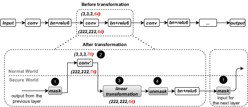
Figure 1: An overview of ShadowNet transformation on a simple CNN.

This CNN is a stack of convolutional layers and each convolutional layer (conv) is followed by a batch normalization (bn) layer and a ReLU6 (relu6) activation layer. The shapes of the weights are marked on the top of the box and the shapes of the outputs are marked under. The red color indicates the change in shape after the transformation. For each convolutional layer (conv), the ShadowNet transformation works in four steps. After the transformation, the conv’ runs in the Normal World, the other layers run in the Secure World.

III Design Overview

III-A Design Goals

Our secure on-device model inference system has the following design goals:

• Security that is rooted in the hardware so that the model remains secure even when the OS is compromised;

• Performance efficiency for supporting real-time analysis;

• Access to hardware accelerators for supporting on-device ML tasks.

III-B Threat Model

We consider a strong adversary who controls the Normal World (including the OS) and observes everything that is exposed to the Normal World (including the GPU tasks). Our primary goal is to protect the model privacy. Specifically, the adversary should not learn anything about a model, $\mathcal{M}(\cdot)$, beyond what is revealed by its querying API, i.e. $Y=\mathcal{M}(X)$. A formal security analysis is presented in Sec. VI-D. We do not consider model inference integrity which can be achieved via verification techniques as proposed in Slalom [70]. Additionally, we do not consider side channel attacks on the TEE – we assume that the TEE can protect the confidentiality and integrity of the program and data inside it. Hence, for loading the model into the TEE all standard attestation techniques apply (such as, loading an encrypted model and decrypting it inside the TEE) and this is orthogonal to ShadowNet’s design.

III-C Design Challenges

While TEEs provide hardware-level security, using mobile TEEs for secure model inference has several technical challenges. First, mobile TEEs, such as Arm TrustZone, are designed for small security critical services, such as managing encryption keys. The memory reserved for the TEE OS is limited. For example, only 14 MB is available for trusted applications of OP-TEE OS on Hikey960 Dev Board while the model size of ResNet-404 is 28 MB. Hence, it is not feasible to run the resource-intensive model inference task inside the TEE (see Sec.VII). Second, current TEEs do not include the GPU/NPU inside the secure domain. Hence, we would lose access to hardware acceleration. Third, the model inference framework would also significantly increase the TCB size.

III-D Our Solution: ShadowNet

The key idea of ShadowNet is as follows:

Example Application. We use a simple example to show how ShadowNet works on a typical CNN as depicted in Fig. 1. The example CNN is a stack of convolutional layers, and each convolutional layer (conv) is followed by a batch normalization (bn) layer and a ReLU6 (relu6) activation layer.

For each convolutional layer conv, the ShadowNet transformation works in four steps: (1) adds a mask layer to the input; (2) replaces the original conv layer with a transformed conv’ layer; (3) adds a linear transformation layer to restore the result of conv’; (4) unmasks the input. The combination of conv’+linear transformation is equivalent to conv in the original CNN. The combination of mask+conv’+linear transformation+unmask is also equivalent to conv. The batch normalization layer and ReLU6 layer remain unchanged.

The mask and unmask layers in step (1) and step (4), respectively, are introduced to prevent the adversary from observing the original input and output of the outsourced linear layers. Note that we embed the inputs in a field $\mathbb{F}$ via quantization before applying the mask layer. Additionally, all the weights of the convolutional layers are also quantized accordingly. The unmasked output is de-quantized before being forwarded to the non-linear layers (for example, the activation layer). We discuss how these layers are implemented in Sec. IV-C. Note that the conv’ layer has 76 kernels instead of 64 kernels. This is due to the obfuscation ratio, a tunable parameter in ShadowNet. In Sec. IV-D, we explain the rationale behind the choice of this number and how to generate the weights for conv’ layer and linear transform layer.

Figure 2: An example of ShadowNet transformed CNN.

The above example has four convolutional layers. Observe that for the first layer, only the output is masked. For the last layer, only the input is masked. This is because according to our threat model, the input to the first layer (model input) and the output of the last layer (model output) is known to the adversary.

Discussion. In summary, ShadowNet offers a novel model inference system that protects the model weights with a TEE while leveraging the untrusted hardware for acceleration. ShadowNet achieves its goal by transforming the computationally heavy linear layers’ weights and masking their input before outsourcing them to the untrusted world and restoring the results inside the TEE. All the non-linear layers are kept secure inside the TEE. With this design,

• ShadowNet’s security is rooted in the TEE, meeting the first design goal.

• ShadowNet does not introduce any heavy cryptographic operations and our evaluation shows that ShadowNet is efficient – this meets our second design goal.

• ShadowNet is still able to use the accelerators which meets the third design goal.

ShadowNet solves the technical challenges (Sec. III-C) of mobile TEEs by maintaining low memory usage and a small TCB which is detailed in Sec. IV and Sec. V.

IV ShadowNet

In this section, we introduce ShadowNet. First, we explain how ShadowNet applies linear transformation on a broad class of linear layers, namely convolutional, pointwise convolutional, depthwise convolutional, and dense/fully connected layers. Next, we discuss the mask layer for input/output privacy. Finally, we describe an optimized implementation of the linear transformations for ShadowNet.
Notations. Here, we introduce the notations we use for the rest of the paper. $\mathbb{F}$ denotes a field. $X$ and $Y$ denote the input and output of a convolutional layer. $X^{\prime}$ and $Y^{\prime}$ denote the masked input and output. $\hat{W}=\big{[}\hat{w_{1}},\cdots,\hat{w_{n}}\big{]}$ represents the transformed convolution filter corresponding to the original convolution filter $W=\big{[}w_{1},\cdots,w_{n}\big{]}$ where $\hat{w}_{i}\thinspace(w_{i})$ denotes the masked (original) convolution kernel. For a positive integer $n\in\mathbb{N}$, $[n]$ denotes the set $\{1,\cdots,n\}$.

IV-A Quantization

All the transformations in ShadowNet work on a field $\mathbb{F}$. For this, we quantize all inputs and weights of a CNN to integers and embed them in the finite field $\mathbb{Z}_{p}$ modulo a prime $p$ ($p$ is sufficiently large to avoid wrap-around). This step is necessary for providing a formal security guarantee (see Sec. VI-D). Following prior work [70, 43], ShadowNet converts a floating point number $x$ to a fixed-point representation as $\tilde{x}=\textsf{FP}(x;l):=\textsf{round}(2^{l}\cdot x)$. After the computation of the linear layers, we de-quantize $\tilde{x}$ by scaling it by $2^{-l}$.

IV-B Transformation of Linear Layers

ShadowNet relies on linear transformation to obfuscate the weights of the linear layers.

Linear Transformation. Linear transformation is a function $f$ defined on vector spaces $V$ and $T$ over the same field $\mathbb{F}$, $f:V\rightarrow T$. For any two vectors $u,v\in V$ and any scalar $c\in\mathbb{F}$, the following two conditions are satisfied:

$$additivity:f(u+v) =f(u)+f(v)$$ (5)

$$homogeneity:f(cu) =cf(u)$$

Convolutional Layer. A convolutional layer is given by $Y=\mathrm{Conv}(X,W^{T})$ where $X$ and $Y$ denote the input and output, respectively, and $W=[w_{1},\cdots,w_{n}]^{T}$ is the convolution filter. A detailed discussion of convolutional layer is attached in Appendix II-A. Let $F=[f_{1},\cdots,f_{n}]$ be a random filter such that each $f_{i},i\in[n]$ has the same shape as $w_{i}$. Additionally, let $\Lambda$ be a diagonal matrix where the diagonal elements $\lambda_{i}\in\mathbb{F},i\in[n]$ are random scalars. Conceptually, the linear transformation on the convolutional layer in ShadowNets works as follows:

$$\small\begin{split}\hat{W}^{T}&=W^{T}\cdot\Lambda+F\\ \Rightarrow[\hat{w}_{1},\cdots,\hat{w}_{n}]&=[w_{1},\cdots,w_{n}]\begin{bmatrix}\lambda_{1}&&\\ &\ddots&\\ &&\lambda_{n}\\ \end{bmatrix}+[f_{1},\cdots,f_{n}]\end{split}$$ (6)

Thus, each of the kernels are transformed as follows

$$\hat{w}_{i}=\lambda_{i}w_{i}+f_{i}$$ (7)

Hence, from the above transformation (Eq. (6)) and the properties of linear transformation (Eq. (5)), we have:

$$\small\begin{split}\mathrm{Conv}(X,\hat{W}^{T})&=\mathrm{Conv}(X,W^{T}.\Lambda+F))\\ &=\mathrm{Conv}(X,W^{T})\cdot\Lambda+\mathrm{Conv}(X,F)\end{split}\vspace{-2mm}$$ (8)

So, we can compute $\mathrm{Conv}(X,\hat{W}^{T})$ on the untrusted GPU and restore the output $Y$ inside the TEE as follows:

$$\small Y=\big{(}\mathrm{Conv}(X,\hat{W}^{T})-\mathrm{Conv}(X,F)\big{)}\cdot\Lambda^{-1}\vspace{-2mm}$$ (9)

Note that the computation of $\mathrm{Conv}(X,F)$ is done in the Normal World. We discuss an optimized implementation of the above in Sec. IV-D.

Pointwise Convolutional Layer. The scheme for the standard convolutional layer can be directly applied to the pointwise convolutional layer.

Depthwise Convolutional Layer. For depthwise convolutional layers, ShadowNet applies linear transformations on both the input and the kernels. Specifically, we $(1)$ shuffle the sequence of input/kernel channels and $(2)$ obfuscate each input/kernel channel with a random scalar as detailed below.

Assume that the input has $n$ channels. Thus, the depthwise convolutional layer has $n$ kernels, one per channel. Let $w_{i}$ represent the $i$-th kernel of the convolution filter $W$, where $W=[w_{1},w_{2},\ldots,w_{n}]^{T}$. Let $(\lambda_{1},\ldots,\lambda_{n})\in\mathbb{F}^{n}$ be a set of random scalars and $\pi\in S_{n}$ ($S_{n}$ is the group of permutations on $[1,\ldots,n]$) be a random permutation. Additionally, let $P_{\pi}$ be a $n\times n$ permutation matrix corresponding to $\pi$ ($P_{\pi}(i,j)=1$ if $\pi(i)=j$, and $0$ otherwise). We scale and shuffle the sequence of the kernels in $W$ with $\Lambda$ as follows:

$$\small\begin{split}\Lambda&=\begin{bmatrix}\lambda_{1}&&\\ &\ddots&\\ &&\lambda_{n}\\ \end{bmatrix}\end{split}\;P_{\pi}\vspace{-2mm}$$ (10)

We apply the same permutation to shuffle the input channels. The input transformation matrix $A$ is defined as follows:

$$\small\begin{split}A&=\begin{bmatrix}\lambda_{1}^{-1}&&\\ &\ddots&\\ &&\lambda_{n}^{-1}\\ \end{bmatrix}\end{split}\;P_{\pi}\vspace{-2mm}$$ (11)

Thus, for identity matrix $I$, we have:

$$\small A\cdot\Lambda^{T}=I\vspace{-2mm}$$ (12)

Given the transformed weights $\hat{W}=[\hat{w}_{1},\ldots,\hat{w}_{n}]^{T}$, the transformations on the input $X$ and weights $W$ are described as follows:

$$\small\begin{split}\hat{W}^{T}&=W^{T}\cdot\Lambda\\ X^{\prime}&=X\cdot A\end{split}\vspace{-3mm}$$ (13)

Let $Y^{\prime}=\mathrm{DWConv}(X^{\prime},\hat{W}^{T})$. It is easy to see that:

$$\small Y^{\prime}=[\mathrm{DWConv}(x_{1},w_{1}),\cdots,\mathrm{DWConv}(x_{n},w_{n})]P_{\pi}\vspace{-1mm}$$ (14)

Let $P_{\pi}^{-1}$ be the inverse of $P_{\pi}$. We can restore the correct result with the following equation:

$$\small Y=Y^{\prime}\cdot P_{\pi}^{-1}\vspace{-3mm}$$ (15)

Note that both the transformation of the input and the restoration of the result are performed inside the TEE while the depthwise convolution on the transformed filter can be outsourced to the untrusted GPU.

Dense/Fully Connected Layer. Recall that a dense layer can be implemented as a pointwise convolutional layer. Hence, ShadowNet applies the same linear transformation as the one described for the standard convolutional layer.

IV-C Layer Input/Output Privacy

We introduce the mask/unmask layer to protect the input $X$ and output $Y$ of the convolutional layers.

Mask Layer. The mask layer adds a random mask to the input of a convolutional layer which is outsourced to the Normal World. Note that, in a typical CNN, the output of a convolutional layer output will be the input for the next layer. In the offline phase, ShadowNet generates random masks $M$ of the same shape as $X$ inside the TEE. The masked input $X^{\prime}$ is defined as follows:

$$\small X^{\prime}=X+M\vspace{-2.5mm}$$ (16)

$X^{\prime}$ is outsourced to the Normal World for the convolutaional layer with filter $W$. A fresh mask is used for every convolutional layer and for every round of model inference. Since all the values are embedded in a field $\mathbb{F}$, this masking is equivalent to applying a one-time pad [51].

Unmask Layer. After obtaining the masked output $Y^{\prime}$ from the Normal World, the TEE restores the original value via:

$$\small Y=Y^{\prime}-\mathrm{Conv}(M,W)\vspace{-2mm}$$ (17)

where the TEE pre-computes and stores the value of $\mathrm{Conv}(M,W)$ in an offline phase. This masking step is similar to Slalom [70].

Recall from our threat model (Sec. III-B) that the adversary already knows $Y=\mathcal{M}(X)$ where $\mathcal{M}$ is the CNN model. Hence, the input to the first layer (model input) and the output of the last layer (model output) is not masked. This is depicted in Fig. 2. After $Y$ is unmasked inside the TEE, it is de-quantized and then, forwarded to the non-linear layers.

IV-D Optimized Implementation

In this section, we describe how ShadowNet implements the linear transformation for the convolutional layers.

Recall from our discussion in Sec. IV-B that $F$ acts as a mask that protects the weights of the kernels. However, the TEE needs access to $\mathrm{Conv}(X,F)$ for restoring $Y$ (Eq. (9)) – the extra computation for $\mathrm{Conv}(X,F)$ is an performance overhead. This introduces a performance/security trade-off which is tackled in ShadowNet as follows:

• First, we select $r\in\mathbb{R},r>1$. We refer to $r$ as the obfuscation ratio and it is a parameter for tuning the performance/security trade-off. We elaborate on this later in this section.

• Select at random $F=[f_{1},\cdots,f_{m-n}]$ where $m=\lceil r\cdot n\rceil$. Each $f_{i}$ has the same shape as that of the kernels of $W$.

• Select a set of $n$ random scalars $(\lambda_{1},\cdots,\lambda_{n})\in\mathbb{F}^{n}$.

• Compute

  $$\small W^{\prime}=[\lambda_{1}w_{1}+f^{\prime}_{1},\dots,\lambda_{n}w_{n}+f^{\prime}_{n},f_{1},\dots,f_{m-n}]^{T}\vspace{-2mm}$$ (18)

  where $f^{\prime}_{i}$s are randomly chosen from $F$. Repetitive choice is allowed here as $m-n$ might be smaller than $n$.

• Store an index matrix $C$ where $C[i]=j$ iff $f^{\prime}_{i}=f_{j}$.

• Finally, shuffle $W^{\prime}$ with a random permutation matrix $P_{\pi}$ for $\pi\in S_{m}$.

  $$\small\hat{W}^{T}=W^{\prime T}P_{\pi}\vspace{-2mm}$$ (19)

All of the above steps can be pre-computed securely in an offline phase. With this transformation, we can easily recover the convolution results with the inverse of the permutation matrix $P_{\pi}$, the index matrix $C$ and the random scalars $(\lambda_{1},\ldots,\lambda_{n})$. Conceptually, the recovery process can be implemented as a pointwise convolution with $n$ filters of shape $(1,1,m)$.

Intuitively, the permutation $\pi$ prevents the adversary from distinguishing between the kernels in $\hat{W}$ that correspond to $F$ and the ones that correspond to (transformed) $W$. Clearly, higher the values of $r$, better is the security and higher is the computational overhead. The formal security and performance analysis is presented in Secs. VI-D and VI-C, respectively. Note that ShadowNet applies the aforementioned transformation to every convolutional layer of the CNN.

Discussion. Here, we discuss how ShadowNet’s design addresses the challenges of mobile TEE as outlined in Sec. III-C. First, ShadowNet tackles the challenge of limited TEE memory by running only a subset of the layers of the model inside the TEE. Specifically, it leaves the resource-heavy linear layers outside the TEE. To further reduce ShadowNet’s computational load, we propose the aforementioned optimized design which reduces TEE’s overhead for restoring the value of the transformed linear layers. Additionally, we propose several novel optimizations for ShadowNet’s implementation to reduce its memory consumption (Sec. V-D). Second, our design of the transformations provides a formal security guarantee (Thm. 1). Consequently, ShadowNet allows efficient outsourcing of the linear layers to the accelerators without compromising on security. Third, the new operations introduced by ShadowNet (for masking and linear transformations) are relatively simple. Hence, ShadowNet’s implementation adds only $2,100$ LOC into the TCB (see Sec. V). Note that TensorFlow Lite has tens of thousands of lines of code and porting it as a whole inside the TEE would require a much larger TCB. ShadowNet, by design, keeps it outside the TCB, thereby supporting its rich functionality in a secure manner with a small TCB.

V Implementation

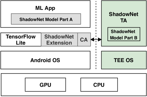
Figure 3: The system architecture of Shadownet on mobile platforms. Color grey shows the part modified by ShadowNet in the Normal World. Color green shows the part in the Secure World. The ShadowNet model part A and B refer to linear and non-linear part, respectively.

V-A Overview of the ShadowNet prototype

We implement the ShadowNet prototype as an end-to-end on-device model inference system as shown in Fig. 3. Our prototype contains the ML mobile application, TensorFlow Lite runtime library with extensions for ShadowNet, ShadowNet client application (CA) and ShadowNet trusted application (TA). ShadowNet runs the transformed linear layers in the Normal World and uses the CA to communicate with the TA in the Secure World, which runs the other (non-linear) layers securely. ShadowNet models are split into two components – Part A and Part B which run in the Normal World and the Secure World, respectively. During inference, Part A, which runs in TensorFlow Lite, processes the linear layers in the Normal World. When executing the non-linear layers, Part A invokes the CA to send commands to the TA which runs Part B inside the Secure World and passes the results back.

V-B Model Conversion

The model conversion mechanism can be divided into two steps as depicted in Fig. 4.

• Step I. The original model (left of Fig. 4) is converted to the ShadowNet model (middle of Fig. 4) with the help of four new layers that transform the weights of the linear layers.

• Step II. All the non-linear layers from the above ShadowNet model (red dotted in Fig. 4) are replaced with a placeholder layer which represents the model in the Normal World and interacts with the Secure World. Now, we have two components of the model – Part A contains the weights of the transformed linear layers and runs in the Normal World (right of Fig. 4) while Part B contains the weights of the other layers in the Secure World (red dotted box in Fig. 4).

Step I. Recall that, convolutional, pointwise convolutional, depthwise convolutional and fully connected/dense layers are considered to be the linear layers. We transform these layers in Step I by introducing four new layers, namely, LinearTransform, ShuffleChannel, PushMask and PopMask. LinearTransform applies a linear transformation to the input. ShuffleChannel scales each channel in the input and shuffles their sequence. PushMask/PopMask adds/removes a mask from its input respectively. In a nutshell,

• Every convolutional layer (including pointwise convolutional and fully connected/dense layers) is replaced with four layers: PushMask layer, transformed convolutional layer, LinearTransform layer and PopMask layer.

• Every depthwise convolutional layer is replaced with five layers: PushMask layer, ShuffleChannel layer, transformed depthwise convolutional layer, ShuffleChannel layer and PopMask layer.

• The weights for the convolutional layers and mask layers are quantized. The outputs from quantized layers are de-quantized accordingly before being forwarded to the non-linear layers.

• The batchnorm layers can be fused with its preceding convolutional layers for the ease of implementation (we do not show it in the example for the ease of exposition).

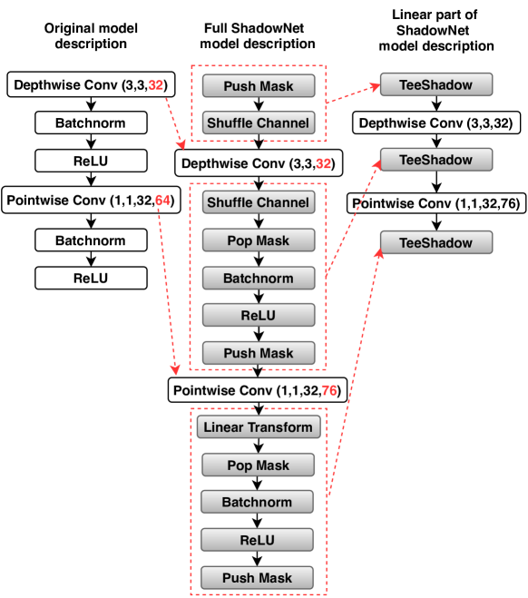
Figure 4: An example of ShadowNet model conversion ($r=1.2$). First, the convolutional layers are transformed. The pointwise convolutional layer’s weight shape changes from (1, 1, 32, 64) to (1, 1, 32, 76), where $76=64\times 1.2$. Next, the linear layers remain unchanged and the non-linear layers are replaced with a placeholder TeeShadow.

Step II. In Step II, we introduce an additional layer called TeeShadow that replaces all the non-linear layers between two successive linear layers. This newly introduced layer serves as a placeholder for the interposed non-linear layers. During model inference, TeeShadow switches to the Secure World to handle the non-linear layers and returns back to the Normal World after its completion. Note that all the newly added ShadowNet layers in Step I as well as the original non-linear layers are placed in the Secure World.

CNNs with shortcuts, such as ResNet [45] and InceptionNet [68], contains branches and merges of different convolutional operations in its data-flow. We address this by introducing a new operation called TeeMerge as shown in Fig 5. Unlike TeeShadow which takes a single input, TeeMerge can take multiple inputs and produce the corresponding output.

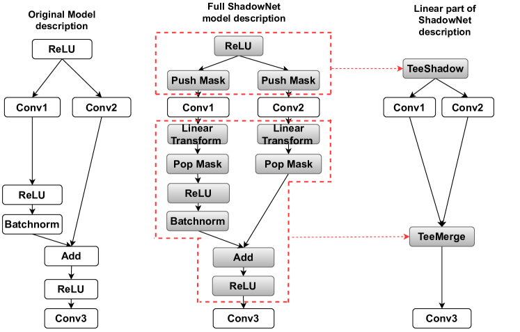
Figure 5: An example of TeeMerge. In the left part of the figure, a shortcut is introduced by ResNet (a convolution is removed from the left branch for simplicity). The middle figure shows the ShadowNet transformed model where the outputs from two different convolutions (Conv1 and Conv2) need to be merged. A new layer, TeeMerge, is introduced to take the inputs from the two branches and generate the corresponding output.

In a nutshell during Step II, the non-linear layers are replaced with TeeShadow layers and the linear layers remain unchanged, as shown in Fig. 4.

V-C Adding ShadowNet Support in TensorFlow Lite

ShadowNet introduces five new operations that are not inherently supported in TensorFlow Lite (TF Lite), namely, LinearTransform, ShuffleChannel, AddMask, TeeShadow and TeeMerge. Note both PushMask and PopMask layers are implemented via AddMask. To implement these operations, we extend TF Lite as follows:

• We implement these operations as CustomOps for TensorFlow.

• We add these CustomOps in the Keras Layer API.

• We add the TF Lite implementations of the CustomOps.

The extension is based on TensorFlow 2.2 which was the latest version at the time of our implementation. To support CustomOp for TensorFlow, we add $563$ LOC in Python, $924$ LOC in C++; to support TF Lite, we add $774$ LOC in C++. Our tool for model conversion is $1223$ LOC in Python.

V-D ShadowNet CA and TA

The ShadowNet CA and TA work as follows. During the initialization phase, the CA starts a secure session with the TA and loads the ShadowNet model Part B into the TA. Before each round of model inference, the CA loads the pre-computed weights for the mask layers into the TA. During model inference, the CA passes the parameters from the TeeShadow operation to the TA and fetches results from it. The TA performs the model inference task for the non-linear layers represented by the TeeShadow (see Fig. 4).

The CA sets up a secure session with the TA and passes the parameters. The ShadowNet TA is implemented as a lightweight and generic model interpreter that can parse the model binary (Part B), and run partial model inference based on the CA’s parameters. It can handle any model in the TensorFlow Lite format (flatbuffers).

We add $480$ and $2,100$ LOC in C for the CA and the TA, respectively. Specifically, the new operations (LinearTransform, AddMask, ShuffleChannel) add $<200$ LOC in the TCB as they are relatively simple operations.

V-E Optimizations

CA and TA’s communication. The OP-TEE OS is designed to work with a TA with a relatively small TEE memory usage ($<1$MB). As a result, for every call the CA makes to the TA, the TEE OS sets up a page mapping for the entire memory used by the TA even when the CA and the TA are in the same session. This has an adverse effect on the performance – when the TA’s memory size increases, the associated cost of the CA’s call to the TA increases proportionately even when the TA is idle inside the TEE. For example, the time increase from 0.1ms to 6ms for a memory increase of 1MB to 64MB. This TEE design limitation is known to be a major challenge in the general OP-TEE community [18, 19]. In order to tackle this, we propose a novel optimization as follows. Note that only the parameters (handles for the memory shared between the CA and the TA) of the CA’s call change and require a new mapping each time – the majority of the TA’s memory, namely the data and code, do not need to be re-mapped for every call. Based on this observation, we implemented an optimization in the TEE OS to cache the page mapping for the TA’s code and data section. Only the pages corresponding to the parameters passed between the CA and the TA are re-mapped. This improves the performance significantly. For instance for ResNet-44, the ShadowNet model inference time reduces from $106$ms to $57$ms – a $2\times$ improvement. We believe that our key idea of caching certain pages could be of independent interest to the broader OP-TEE community.

Optimizing TA’s Memory Management. The TEE OS has a limited memory reserved for the TA. Without careful memory management, the TA would exhaust the memory and crash. We tackle this challenge as follows. First, we allocate memory statically in the TA to avoid fragmentation caused by dynamic memory allocation. Specifically, for a given model, the memory needed for each layer can be determined at the time of loading and allocated statically. Second, we do not allocate memory for the output of each layer. Instead, we allocate two sufficiently large buffers and rotate them to save memory.

Optimizing TA’s Performance. Implementing the TA in OP-TEE has many restrictions. For example, since OP-TEE only supports C, we would lose access to popular compute libraries, such as Eigen[11] and Arm Compute Lib [4] in C++. Additionally, OP-TEE lacks a math library. Hence, we propose efficient implementations of mathematical functions, such as sqrt, exp, or tanh, for the non-linear layers.

TABLE II: Optimizations of the TA (with MobileNets model)

Optimizations	Exec. Time (ms)
Baseline (Static mem. alloc)	1500
(1) Neon sqrt	300
(2) Cache friendly	245
(3) Optimize loop sequence	205
(4) Preload weights	100
(5) Neon for Batchnorm, AddMask	90
(6) Neon for ReLU6	81

Note: The optimizations are applied incrementally in a sequence. For example, $81$ms is the execution time inside the TA (excluding mask weights reloading time) when optimizations (1) to (6) are all applied.

Initially, we ported the non-linear layers from Darknet [60], a deep learning framework for desktop written in C. However, the resulting TA was very slow on our Arm64 Dev Board. Hence, we propose the following optimizations to bring the performance at par with that of TensorFlow Lite.

• Use Arm Neon to optimize the sqrt implementation in the Batchnorm layer.

• Swap the inner and outer loops when necessary to support cache-friendly data access for multi-dimensional data.

• Move repetitive computation out of the loops and pre-compute it.

• Pre-load all the weights to avoid repetitive loading.

• Use Neon multiply+add instructions to optimize the Batchnorm and AddMask operations.

• Use Neon minimum/maximum instructions to optimize the activation layers, such as ReLU6.

Table II shows the execution times for our proposed optimization for the MobileNets TA. An illustration of the sqrt optimization is presented in App. A

Configuration of the TEE OS. We also increase the size of the secure memory reserved for the TEE OS from 16MB to 64MB to accommodate a larger Part B. Additionally, we changed the size of the reserved shared memory from 2MB to 8MB. This shared memory is used for communications between the Normal World and the Secure World. These changes only require a few lines of configurational code in the TEE OS and Arm Trusted Firmware. No change is required in the Normal World OS, such as Android/Linux.

VI Evaluation

Our evaluation focuses on four questions:

• Correctness: Does ShadowNet produce the same result as the original model?

• Efficiency: What is the overhead introduced by ShadowNet?

• Obfuscation Ratio: What is the impact of the obfuscation ratio on the correctness and performance of ShadowNet?

• Security: How secure is ShadowNet?

Configuration. We perform the evaluation on the Hikey960 [1] board equipped with Kirin 960 SoC with 4 Cortex A73 + 4 Cortex A53 Big.Little CPU architecture, ARM Mali G71 MP8, and 3GB LPDDR4 SDRAM. We run Android P in the Normal World and OP-TEE OS 3.9.0 [17] in the Secure World. We use the field $\mathbb{Z}_{p}$ for prime $p=2^{24}-3$ and a fixed-point representation of $l=8$ for quantization. The obfuscation ratio is set to be 1.2.

Models. We evaluate ShadowNet on five popular models – MobileNet [15], ResNet-44 [21], ResNet-404 [20], YOLOv4-tiny [31] and MiniVGG [14]. The rationale behind choosing these models is that they cover a wide range of CNN architectures. MiniVGG is derived from VGG which represents a classical CNN architecture. MobileNet uses pointwise and depthwise convolution which are convolutional layers customized for mobile devices. ResNet uses shortcut connections between the convolutional layers which create branches and merges in the network structure. YOLOv4-tiny is an object-detection model with a complex CNN architecture. First, object detection requires a multi-task model/multi-objective optimization which outputs a prediction class and a bounding box. Second, the model structure is non-sequential with new activation operations, such as LeakyRelu [61], and complicated Lambda layers consisting of different non-linear operations, such as upsampling, concatenation. Third, the original model size is 34MB which is large in the context of mobile environments.

Datasets. MobileNet is evaluated on the ImageNet-2012 dataset [64] with 50K images. ResNet-44, ResNet-404 and MiniVGG are evaluated on the CIFAR-10 dataset [52] with 10K images. We evaluate YOLOv4-tiny on the VOC2007 testing dataset [39].

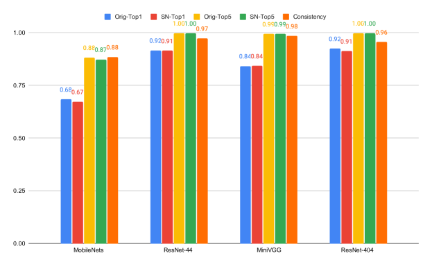
Figure 6: Prediction accuracy and consistency evaluation. Orig-Top1 refers to the original model’s top-1 accuracy, SN-Top1(5) refers to the top-1(5) accuracy of the ShadowNet transformed model. Consistency measures the % of ShadowNet predictions that match with that of the original model.

VI-A Correctness

We evaluate the correctness of ShadowNet by comparing the prediction accuracy and consistency before and after model transformation. Consistency checks whether ShadowNet top-1 prediction is consistent with the original model on the same input. Fig. 6 shows our evaluation results on four models – MobileNet, ResNet-44, ResNet-404 and MiniVGG. For YOLOv4-tiny, we calculated mean average precision (mAP) based on 50% Intersection Of Union which is the standard metric for object detection. The accuracy of the original model and ShadowNet is $57.06\%$ mAP and $55.90\%$ mAP, respectively. Our implementation is based on the pre-trained model from [31]. Overall, we observe that ShadowNet has accuracy comparable to that of the original models ($\sim 1\%$ decrease is due to the numerical errors from quantization – an essential step for security).

ShadowNet is $94\%$ consistent for YOLOv4-tiny. ShadowNet’s Top1 prediction consistency for ResNet-44, ResNet-404, MiniVGG and MobileNet are $97\%$, $96\%$, $98\%$ and $88\%$, respectively. The relatively low consistency for MobileNet is due to the inputs which are predicted incorrectly by the original model. Specifically for inputs with correct predictions from the original model, ShadowNet is $95\%$ consistent; for the incorrect predictions, ShadowNet is $74\%$ consistent. The original model’s mean confidence (top-1 score) for the inputs with correct and incorrect prediction is $0.8$ and $0.38$, respectively. Recall that MobileNet is evaluated on ImageNet with 1K classes. Hence for classification tasks with such a large number of classes, ShadowNet’s numeric errors can impact inputs that have low confidence scores from the original model (for instance, the top-2 scores are very close). The performance is acceptable since this affects mostly the inputs with incorrect predictions from the original model.

VI-B Efficiency

We use the model inference time as our metric which measures the time span between feeding an image and getting the classification result.

Experimental Highlights. Our evaluation shows that:

• ShadowNet results in a reasonable overhead, increasing the model inference time by $0.6\times$ to $1.6\times$.

• GPU acceleration can reduce the model inference time for all three models from $1$ms to $30$ ms. There is still a large room for improvement with software and hardware updates.

Methodology. We use the TensorFlow Lite Android image classifier Demo application [26] developed by Google to evaluate the end-to-end model inference time. We evaluate ShadowNet under different settings – (1) the original model on CPU; (2) the ShadowNet transformed model on CPU; (3) the original model on GPU; (4) the ShadowNet transformed model on GPU.
Fig. 7 shows the model inference time for ShowdowNet.

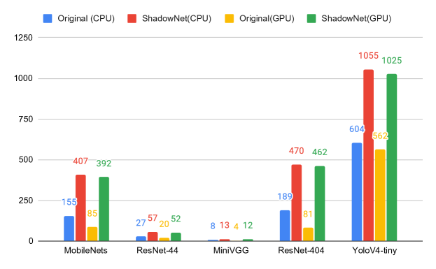
Figure 7: ShadowNet performance evaluation (ms). We evaluate ShadowNet on five CNN models: MobileNet, ResNet-44, MiniVGG, ResNet-404 and YOLOv4-tiny ($r=1.2$). For each model, we measure the model inference time for one image on four different settings: original model on CPU, ShadowNet model on CPU, original model on GPU and ShadowNet model on GPU. We report the mean of 100 trials.

ShadowNet’s Performance on CPU. Compared with the original model in the CPU mode, ShadowNet incurs an overhead of 252ms $(1.6\times)$, 30ms $(1.1\times)$, 5ms $(0.6\times)$, 281ms ($1.5\times)$ and 451ms $(0.7\times)$ for MobileNet, ResNet-44, MiniVGG, ResNet-404 and YOLOv4-tiny, respectively. The overhead is reasonable as ShadowNet refreshes the masks for each round of model inference. Table III shows the model size before and after the ShadowNet transformation. For example, for MobileNet, the weights of the mask layers has a size of $37$MB which takes around $200$ms to be updated. For ResNet-$44$, the mask size is $3.3$MB which takes $18$ms to be updated.

TABLE III: ShadowNet model size change.

Model Size(MB)		MobileNet	ResNet-44	ResNet-404	YOLOv4-tiny	MiniVGG
Original Model	Conv	17	2.43	24.71	22.56	20
	Other	0.175	0.029	0.23	0.79	0
ShadowNet Model	Conv	20	2.92	29.79	27.11	24
	Other	37	3.3	29.73	40.53	2

Model weights are divided into two parts – Conv layers’ weights (standard convolutional, pointwise convolutional, depthwise convolutional and dense layers) and Other layers’ weights (AddMask, LinearTransform, ShuffleChannel, Batchnorm). Among the Other layers, the weights of the AddMask layer occupy the maximum space for ShadowNet models.

Despite having an additional 5ms to 451ms latency depending on the original model size, we find that the impact on the user is acceptable. We test this by running Demo to detect objects in real-time. For MobileNet, Demo processes around six images per second for the original model, and two and a half images for ShadowNet. For small models, such as MiniVGG, the extra $5$ms latency is imperceptible to users.

Performance Impact from GPU. Running on GPU reduces model inference time by 15ms (4%), 5ms (9%) and 1ms (8%), 8ms (2%), 30ms (3%) for MobileNet, ResNet-44, MiniVGG, ResNet-404 and YOLOV4-tiny, respectively. The benefit of GPU acceleration for ShadowNet model is not as good as that for the original models due to the following reasons. First, the GPU speedup ($\sim 2\times$) on our evaluation board is significantly less than the GPU speedup in the cloud. Any advancement in on-device GPUs would immediately improve ShadowNet’s performance. Second, ShadowNet requires splitting the model inference between the CPU (TEE mode) and the GPU. The interleaving between the CPU and the GPU causes extra overhead for repeated setting up of the GPU jobs.

We would like to remark that mobile GPU acceleration for on-device ML is still a developing research area [9]. Hence, ShadowNet’s benefit is that it opens the door for leveraging future advances in on-device accelerators.

Offline Time. Offline model conversion takes $10$min $59$s for MiniVGG, $6$min 5s for ResNet-44, $31$min $23$s for MobileNet, $28$min $46$s for ResNet-404, $24$min $23$s for YOLOv4-tiny. Regeneration of mask layers’ weights for $100$ instances takes $2.19$s for MiniVGG, $20.29$s for ResNet-44, $97.26$s for MobileNet. $127.9$s for ResNet-404, $25.5$s for YOLOv4-tiny.

VI-C Obfuscation Ratio

Fig. 9 shows how the accuracy, size and inference time of the MobileNet model vary with $r$. We observe that both top1 and top5 accuracy remain almost unchanged as $r$ varies from $1.0$ to $2.0$. This shows that ShadowNet’s accuracy does not depend on the obfuscation ratio. Another observation is that the model size increases linearly with $r$ and so does the model inference time. This is intuitive because both the weight size and the amount of computation for the convolutional layers grow linearly with $r$. See Sec. VI-D for more discussion on how to choose $r$.

VI-D Security Analysis

Adversary’s view of ShadowNet Input: $X_{1}$   View (Normal World): $\hat{W}_{i}$, $i\in[k]$ $X^{\prime}_{i}=Y_{i-1}+M_{i}$, $i\in[2,k]$   Output: $Y_{k}$, output of the model   Goal of Adversary: Find weights of $W_{i}$, $i\in[k]$

Figure 8: Formalization of the adversary’s goal. Let $\mathcal{M}(\cdot)$ denote a CNN with $k$ convolutional layers. Given input $X_{1}$ (input to the first layer), the model’s output is $Y_{k}$ (output of the last layer). The input of $i$-th layer is the output of the previous layer, i.e., $X_{i}=Y_{i-1},i\in[2,k]$. For ShadowNet, $X^{\prime}_{i}$ denotes the masked input for the $i$-th layer which is given $Y_{i-1}+M_{i}$. For each convolutional layer, the adversary can observe the masked input $X^{\prime}_{i}$ and the transformed filter $\hat{W}_{i}$. The adversary’s goal is to find the original weights of $W_{i}$.

In this section, we present the formal security analysis of ShadowNet. Let us consider a CNN with $k$ standard convolutional layers where $W_{i}$ denotes the convolution filter for the $i$-th layer. Additionally, $X_{i}$ ($Y_{i}$) denote the input (output) for the $i$-th layer. For a transformed filter $\hat{W}$, let $\mathcal{F}(\hat{W})$ represent the set of filters that could have been transformed to $\hat{W}$, i.e., the set of possible pre-images for $\hat{W}$. We call this the feasible set for $\hat{W}$. The exact construction of $\mathcal{F}(\hat{W})$ is detailed in App. B. The view of the adversary is equivalent to that of the Normal World and is illustrated in Fig. 2.

Theorem 1.

For a CNN with $k$ convolutional layers and a given view of the normal world $\textsf{View}_{\textsf{Normal}}=\big{(}X_{1},Y_{k},\hat{W}_{1},\cdots,\hat{W}_{k},X^{\prime}_{2},\cdots,X^{\prime}_{k}\big{)}$, we have:

$$\small\forall i\in[k],\forall(W^{\prime},W^{\prime\prime})\in\mathcal{F}(\hat{W_{i}})\times\mathcal{F}(\hat{W_{i}})$$ (20)

$$\mathrm{Pr}\big{[}W_{i}=W^{\prime}|\textsf{View}_{\textsf{Normal}}\big{]}=\mathrm{Pr}\big{[}W_{i}=W^{\prime\prime}|\textsf{View}_{\textsf{Normal}}\big{]}$$ (21)

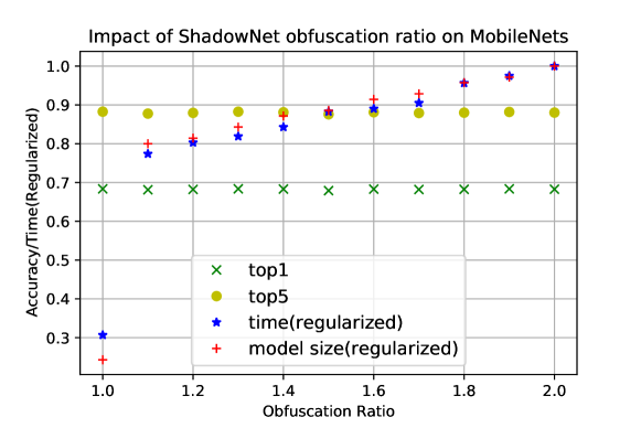
Figure 9: Analysis of performance with varying obfuscation ratio. We measure the change in accuracy (top1 and top5), size (regularized) and inference time (regularized) with the obfuscation ratio, $r$, (ranging from 1 to 2) for MobileNet. Here, $r=1$ refers to the original model and is treated as the baseline.

Proof Sketch.

Every input/output pair for the intermediate layers $i\in[2,k-1]$ is embedded in $\mathbb{F}$ and masked. As a result, $X^{\prime}_{i}$ is indistinguishable from a randomly chosen input of the same shape in $\mathbb{F}$. Hence, $X^{\prime}_{i}$s clearly contain no information about the convolution filters. For the first (last) layer, the output (input) is masked which also prevents any reconstruction of the true weights for $W_{1}$ ($W_{k}$). The rest of the proof follows trivially from the construction of the feasible sets $\mathcal{F}(W_{i})$. The full proof is presented in App. B. ∎

The above theorem states that, on observing a transformed filter $\hat{W}_{i}$, corresponding to any convolutional layer $i$, an adversary cannot distinguish between two filters that belong to its feasible set. Thus, the feasible sets act as cloaking regions for the original weights. Intuitively, the parameter $r$ is analogous to the security parameter (such as, key size) for generic cryptographic protocols. The larger the value of the obfuscation ratio $r$, the greater is the size of the feasible set and consequently, the better is the security. Concretely, $\mathcal{F}(\hat{W}_{a})\supset\mathcal{F}(\hat{W}_{b})$ where $m_{a}=|\hat{W}_{a}|>|\hat{W}_{b}|=m_{b}$ (equivalently, $r_{a}>r_{b}$). $r$ is essentially a trade-off between the security guarantee and performance. The exact size of feasible sets can be analytically computed (see App. B). Fig. 9 shows ShadowNet’s performance with varying values of $r$. Based on this, we set $r=1.2$ for our experimental setup since this was the sweet spot. Specifically, even with $n=16$ (smallest $n$ for our evaluation) and field $\mathbb{F}=\mathbb{Z}_{p}$ for $p=2^{24}-3$, the size of the feasible set, $|\mathcal{F}(\hat{W})|$, is of the order of $2^{268}$ which is sufficient for security. The reason why we get a large feasible set even with a relatively small value of $r$ is that the random permutation matrix $P_{\pi}$ and random scalar multiplications by $\lambda_{i}$s also contribute significantly to the size of the feasible set.

Note. In the above guarantee, the formal security of the mask layers is rooted in the quantization step. Specifically, the quantization operation embeds the value in a finite field, $\mathbb{F}$. Subsequently, the masks can be chosen uniformly at random from $\mathbb{F}$ thereby making the mask layer equivalent to one-time-pad encryption [63].

Based on Thm. 1, we present the following conjecture:

Conjecture 1.

Let $q$ be the number of queries required for a model stealing attack with access to just the querying API, i.e, $Y=\mathcal{M}(X)$ (black-box model stealing attack) and some information about the model architecture (such as, number and type of convolutional layers). Let $q^{\prime}$ be the number of queries required for an attack on ShadowNet. We conjecture that $q^{\prime}$ is of the order of $O(q)$.

Black-box model stealing attacks can be typically classified into two types – $(1)$ functionally-equivalent model stealing attacks [47] where the attacker tries to extract the exact weights of model by analytically solving a set of linear equations, $(2)$ learning-based model stealing attacks where the adversary tries to learn a shadow model [71, 59, 57, 33]. The first type of attacks are impossible in ShadowNet – since our mask layers are refreshed every time, it is mathematically impossible to solve for the model weights (Lemma 2, App. B). Clearly from our threat model (Sec. III-B), protection against learning-based black-box model stealing attacks is beyond the scope of ShadowNet. The implications of Conjecture 1 in this context is that with ShadowNet, an adversary cannot do anything significantly better than a standard learning-based black-box model stealing attack. Our reasoning is based on the fact the feasible sets for the transformed weights are sufficiently large – this provides sufficient cloaking region for the original weights. In other words, an adversary cannot learn anything useful about the original weights by observing the ShadowNet transformed weights. We provide empirical evidence in support of our conjecture as follows.

Empirical Analysis. Table IV shows the empirical evaluation of our conjecture based on two black-box attacks, namely, Knockoff attack  [57] and MixMatch [33, 47], on a victim model of a four layer fully-connected CNN trained on CIFAR-10 (Fig. 2). Knockoff is the state-of-the-art black-box attack with an adaptive query strategy. A recent survey [38] shows that MixMatch is currently the state-of-the-art attack with the highest attack accuracy. Knockoff queries the victim model from an out-of-distribution dataset. For our evaluation, Knockoff uses 10K queries from CIFAR-100 [8] selected via an adaptive strategy based on reinforcement learning. MixMatch is based on semi-supervised learning; the attack samples 8K points from CIFAR-10 for querying the victim model and uses an additional 8K unlabeled points from CIFAR-10 for its semi-supervised training. For Knockoff, the victim model is trained on CIFAR-10 with accuracy 81.6% (column 1 in Table IV). For MixMatch, the victim model is trained on CIFAR-10 with the MixMatch semi-supervised training approach and has accuracy 98.1% (column 1). We used different training strategies for the victim model for the two attacks in order to be consistent with the configurations of their respective original papers [16]. The baseline shadow model (column 2) for Knockoff and MixMatch is and ResNet-18 and Wide-ResNet-28, respectively.

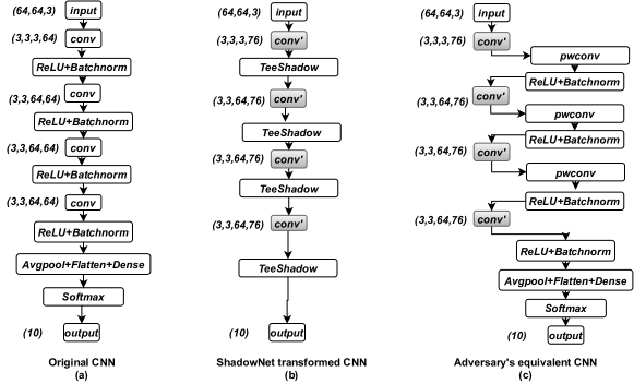
Figure 11: Figure (a) shows the original CNN model. Figure (b) is the ShadowNet transformed model. Figure (c) the adversary’s equivalent CNN. Before training, its conv’ layers are initialized with weights copied from the corresponding conv’ layers of the ShadowNet transformed model. These conv’ layers are then reused by the adversary and marked as non-trainable during training.

In order to assess whether the adversary benefits from knowing the transformed weights ($\hat{W}$) in ShadowNet, $(1)$ we create a custom adversary model with the same architecture as that of the victim model, $(2)$ we copy weights $\hat{W}$ to the adversary’s model, $(3)$ we mark the convolutional layers with weights $\hat{W}$ as non-trainable and train only the other layers (results in column 3). The resulting adversary model is depicted in Fig. 11 in App. B. We observe that the ShadowNet adapted attack is less accurate than the baseline attack (column 2) after the same number of queries. In fact, it performs worse than a random baseline (column 4) where the weights of the non-trainable convolutional layers (as described above) are randomly assigned. This shows that the ShadowNet transformed weights contain no useful information about the original weights and the adversary gains no advantage by reusing the transformed weights.

TABLE IV: Empirical evaluation of black-box attack

	Victim	Attack Baseline	ShadowNet	Random Baseline
Knockoff [57]	81.6%	36.6%	31.1%	36.2%
MixMatch [33, 47]	98.1%	95.8%	92.3%	92.4%

Column 1 reports the underlying victim model’s accuracy. Column 2 corresponds to the attack baseline where the adversary has no knowledge of the victim model. Column 3 corresponds to the attack setting adapted for ShadowNet where the adversary has access to the victim model’s transformed weights. Column 4 corresponds to the case where the convolutional layers of the attacker’s model have random weights.

VII Discussion

Running unmodified model inside the TEE. There are several challenges in running the unmodified model inside the TEE. First, standard model inference (outside the TEE) is memory intensive relative to the original model size. For instance, the original model size for MiniVGG and ResNet-44 is 20MB and 2.4MB, respectively. However, running the unmodified model inference requires dynamically allocating at least 44MB (2.2X) and 10MB (4.2X) for MiniVGG and ResNet-44, respectively. This is because running convolutional layers for standard model inference requires reshaping a 3D weight matrix into 2D matrices – this needs large chunks of intermediate dynamic memory allocation to store the extra copy of the resized weights. In contrast, ShadowNet only requires 4MB (0.2X) and 5MB (2.1X) TEE memory for MiniVGG and ResNet-44, respectively. ShadowNet reduces the memory footprint by keeping the memory-intensive linear layers outside the TEE. ShadowNet’s memory requirement for MobileNets (original model size 17.2MB) is relatively high (48MB -2.7X) since the MobileNets architecture introduces special CNN layers such as depthwise and pointwise convolution which increases the size of the input and output for each layer. As a result, the mask layer added by ShadowNet consumes a relatively larger amount of TEE memory. Nevertheless, it is still significantly lower than running the unmodified model inside TEE (61MB-3.5X). Second, running unmodified models inside the TEE would require a significant engineering effort. TensorFlow Lite needs to be ported into the TEE to support the convolutional layers and matrix operations which rely on certain mathematical libraries (in C++) for efficiency. This entails a significant engineering effort since currently Arm OP-TEE OS does not support C++ and its associated computing libraries. Third, the limited size of the TCB presents additional challenges. TensorFlow Lite has tens of thousands lines of code and porting it as a whole inside TEE would require a much larger TCB. On the other hand, recall that ShadowNet can work with a small TCB – its TA adds only 2100 LOC inside the TEE (the new operations add $<200$ LOC inside the TCB). Additionally, note that the extra code added for model conversion is used offline by the model vendor and is not deployed on the device. Hence, this does not increase the on-device TCB size. Last, we will lose access to hardware accelerators if we run the unmodified model inside the TEE.

Figure 10: Proof-of-concept transformation on LSTM. The original LSTM layer is showed on the top and the ShadowNet transformed LSTM is depicted at the bottom. The red circles represent pointwise matrix operations and the yellow square boxes marked with activation symbols represent fully connected layers followed by the corresponding activation layers. Green boxes marked “LT”, “PUSHM” and “POPM” represent the “LinearTransform”, “PushMask” and “PopMask” layer of ShadowNet, respectively. The yellow square boxes marked with “CONV^′” represent the ShadowNet transformed convolutional layers which are outsourced to the untrusted world. All the other parts of the LSTM layer including the internal states remain in the secure world.

Support for CNNs and LSTMs. In general, ShadowNet can be applied to any CNN model as long as the TEE can support the memory requirements of the corresponding ShadowNet transformed model. The amount of TEE memory required for running the ShadowNet transformed model can be estimated by the size of the weights that need to be stored inside the TEE (Other in Table III). Concretely, the total size is given by the sum of the size of the weights of four ShadowNet operations, namely, LinearTransform, ShuffleChannel, AddMask and Batchnorm. The size of LinearTransform and ShuffleChannel can be computed from the shapes of the convolutional layer and the obfuscation ratio. The size of AddMask can be computed from the input and output shape of each layer. The size of Batchnorm can be computed directly from the model.
ShadowNet can also be used for LSTMs. LSTMs typically consist of fully-connected layers, pointwise matrix operations and activation layers. Recall that a fully connected layer can be treated as a convolutional layer during the ShadowNet transformation. Hence for LSTMs, ShadowNet applies linear transformation on the fully connected layers while keeping the pointwise matrix operations and activation layers inside the TEE. As a concrete example, a LSTM layer (top) and its corresponding ShadowNet transformation (bottom) is depicted in Fig. 10. We implement a prototype ShadowNet transformation for the LSTM layer depicted in Fig. 10 with an input ($x_{t}$) shape of $(12,30)$, output space/units set to be $10$, obfuscation ration $r=1.2$ and $1640$ parameters. The number of parameters after the ShadowNet transformation is $3640$ – the extra parameters are due to the mask layers and the transformed CONV^′ layers. Original LSTM model inference time is 33 ms while the Shadownet transformed LSTM model inference time is 41ms (1.24X).
Support for Cloud Platform. ShadowNet can be used for secure model inference in the cloud as well. For this, the ShadowNet CA/TA needs to be changed to support a cloud TEE, such as SGX. Compared with other designs that perform model inference inside SGX [53, 27], we expect ShadowNet to be more efficient in using the SGX memory and to benefit from the co-located GPUs for acceleration.
Layerwise ShadowNet. ShadowNet transformations can be applied on each convolutional layer independently. Hence, an alternative strategy for implementation is to selectively apply ShadowNet to only the sensitive layers which would improve performance. The rationale behind Layerwise ShadowNet is supported by research on transferable learning [74] which shows that the bottom layers contain features that are more specific to the training dataset. Hence, these features are more sensitive than the generalized features in the top layers.

VIII Related Work

Existing research on secure ML covers both end devices and cloud-based solutions. Offline Model Guard (OMG) [32] provides a secure model inference framework for mobile devices based on SANCTUARY [35], a user space enclave built on Arm TrustZone. However, the original paper presents only a proof-of-concept implementation for OMG that cannot be directly integrated with existing mobile apps (unlike ShadowNet). Moreover, OMG is based on the Sanctuary enclave [35] which runs a user application along with the OS in an isolated environment. For model inference, the unmodified model is run inside the Sanctuary enclave. Thus, the threat model is different as OMG requires the whole software stack, including the OS, libraries and the application inside Sanctuary, to be trusted. ShadowNet, on the other hand, relies only on a secure TEE-OS and TA which is a more relaxed trust assumption. MLCapsule [44] also deploys the model on the client side to protect the user input from being sent to the untrusted cloud. Additionally, it runs the model inference inside SGX to prevent the model from being leaked to the client. DarkneTZ [56] is a secure machine learning framework built on top of Arm TrustZone. It allows a few selected layers to run inside the TEE to protect part of the model. OMG, MLCapsule and DarknetTZ do not support secure GPU acceleration and have a larger TCB size than ShadowNet. Graviton [72] proposes TEE extension for GPU hardware, thus allowing GPU tasks to run securely. However, it requires hardware changes to the GPU. Secloak [54] partitions the GPU into Secure World to run GPU tasks securely at a high performance penalty. ShadowNet does not change the GPU hardware or partition the GPU into the Secure World.

TensorSCONE [53] proposes a secure ML framework that runs on the untrusted cloud. However, it is only evaluated on Inceptionv4 and has a 3.1X time overhead with 330MB memory consumption – these overheads are higher than that of ShadowNet. Additionally, it is designed for a cloud environment while ShadowNet is aimed at a mobile environment which is more resource constrained. TF Trusted [27] leverages custom operations to send gRPC messages to the Intel SGX device via Google Asylo [6].This requires more TEE resources than ShadowNet and does not support GPU acceleration.

Slalom [70] outsources the linear layers to the GPU for acceleration with masked inputs while keeping the other layers inside SGX. Slalom protects the user input privacy but not the model weights from the untrusted server while ShadowNet protects the model weights. YerbaBuena [42] partitions the model into frontnets and backnets, and executes the frontnets inside SGX. This protects the input from the cloud. SecureNets [37] transforms both the input and the linear layer into matrices and applies matrix transformations [65] before sending them to the cloud. It is unclear whether SecureNets supports depthwise convolution and convolution with stride. ShadowNet does not require transforming input and weights into matrices and is compatible with existing linear operations.

Some secure ML systems use cryptographic primitives, such as CryptoNets [41], [49], TF Encrypted [25] and SafetyNets [40]. ShadowNet’s performance is orders of magnitude better than such cryptographic approaches. For instance, for a single image classification, CryptoNets takes $\sim$570s s on a PC while ShadowNet takes $<$1s on a smartphone.

IX Conclusion

In this paper, we have proposed ShadowNet, a secure on-device model inference system for CNNs that protects the model privacy with a TEE while leveraging the untrusted hardware for acceleration. We have implemented an end-to-end prototype of ShadowNet on TensorFlow Lite and OP-TEE with optimizations to work with a small TCB.

Appendix A Optimizing the sqrt function

TABLE V: Performance of different sqrt implementation.

Sqrt Impl.	Time(ms)	S/H	Algorithm	CFLAG
GNU libc	3.53	S	IEEE754	Default
Newlib	13.78	S	IEEE754	-O2
Our TA	194.04	S	Newton	-Os
Arm VFP	10.86	H	unknown	Default
Arm Neon	6.62	H	Newton	Default

Note: a. S/H: S means Software based implementation, H means Hardware based implementation, like special instructions; b. CFLAG: GCC compilation flag; c. IEEE754 means algorithm exploits bits hacking of IEEE754 float format; d. Newton means Newton Iteration for sqrt.

There are many different implementations of the sqrt function for floating point numbers for AArch64 architecture. Software-based implementations include algorithms using Newton iteration and bits hacking of IEEE754 float representation. Hardware-based implementations include Arm VFP support for fsqrt, and Arm Neon support for float sqrt. Additionally, the performance of software-based implementations is also affected by the compilation flag. The default gcc compilation flag for TA is -Os, which optimizes space first; if we change it to -O2, the performance is more than 100x faster while the TA size increases from 55KB to 67KB. We evaluate all the above implementations by doing 3,200,000 sqrt operations and show the results in Table V. Our TA initially used a software implementation using Newton Iteration algorithm. After evaluation, we switched to the Arm Neon based sqrt implementation for the speed and ease of implementation.

Appendix B Security Analysis

Construction of Feasible Set. We refer to the kernels $f_{i}$ in the random filter $F=[f_{1},\cdots,f_{m-n}]$ as mask kernels. Additionally, let $\in_{R}$ represent a uniform random sampling. In what follows, we outline the methodology to compute the feasible set, $\mathcal{F}(\hat{W})$ for a given transformed weight matrix $\hat{W}$. The idea is to back-trace and compute the set of possible pre-images. Now, the feasible set is constructed as follows:

1. Select the set of $m-n$ indices uniformly at random:

   $$\Omega\subset_{R}[m],|\Omega|=m-n$$ (22)

   $\Omega$ represents a possible set of indices that correspond to the mask kernels.

2. The corresponding set of mask kernels is:

   $$\Phi_{\Omega}=\{\hat{w}_{i}|i\in\Omega\}$$ (23)

3. Let $\overline{\Phi}_{\Omega}=\{\hat{w}_{i}|i\in[n]\setminus\Omega\}$ be the set of transformed original kernels. Additionally, let $\overline{W}=[\overline{w}_{1},\cdots,\overline{w}_{n}]$ where $\overline{w}_{i}\in\overline{\Phi}_{\Omega}$ and $\overline{w}_{i}\neq\overline{w}_{j},i,j\in[n],i\neq j$.

4. Sample a random permutation $\sigma\in_{R}S_{n}$. We assume that $\sigma=\pi[1:n]^{-1}$, i.e,, $\sigma$ reverses the effect of $\pi$ on the transformed original kernels. Thus, $\overline{W}_{\sigma}=[\overline{w}_{\sigma(1)},\cdots,\overline{w}_{\sigma(n)}]$ represents a possible transformed filter.

5. Compute

   $$\forall i\in[n]$$

   $$\mathcal{F}^{i}_{\Omega,\sigma}(\hat{W})=\{w|w=d\cdot(\overline{w}_{\sigma(i)}-\hat{w}^{\prime}),d\in_{R}\mathbb{F},\hat{w}^{\prime}\in_{R}\Phi_{\Omega}\}$$

   $\mathcal{F}^{i}_{\Omega,\sigma}(\hat{W})$ represents the set of possible values for the kernel $w_{i}$ for the given $\Omega$ and $\sigma$.

6. Compute

   $$\mathcal{F}_{\Omega,\sigma}(\hat{W})=\big{\{}\big{[}w_{1},\cdots,w_{n}\big{]}\big{|}\forall i\in[n],w_{i}\in\mathcal{F}_{\Omega,\sigma}^{i}(\hat{W})\big{\}}\big{\}}$$

   $\mathcal{F}_{\Omega,\sigma}(\hat{W})$ denotes the set of possible filters $W$ for the given $\Omega$ and $\sigma$.

7. Clearly, we have

   $$\mathcal{F}(\hat{W})=\bigcup_{\Omega}\bigcup_{\sigma}\mathcal{F}_{\Omega,\sigma}(\hat{W})$$ (24)

Clearly, larger the value of $r$, greater is the size of $\Omega$ and consequently, $\mathcal{F}(\hat{W})$. Additionally, it is evident that $\mathcal{F}(\hat{W}_{a})\supset\mathcal{F}(\hat{W}_{b})$ where $m_{a}=|\hat{W}_{a}|>|\hat{W}_{b}|=m_{b}$ (equivalently, $r_{a}>r_{b}$). For depthwise convolutional layer, we have

$$\mathcal{F}(\hat{W})=\{[d_{1}\cdot\hat{w}_{\sigma(1)},\cdots,d_{n}\cdot\hat{w}_{\sigma(n)}]\big{|}\sigma\in_{R}S_{n},\forall i\in[n]~{}d_{i}\in_{R}\mathbb{F}\}$$ (25)

Theorem 1. For a CNN with $k$ convolutional layers and a given view of the normal world $\textsf{View}_{\textsf{Normal}}=\big{(}X_{1},Y_{k},\hat{W}_{1},\cdots,\hat{W}_{k},X^{\prime}_{2},\cdots,X^{\prime}_{k}\big{)}$, we have:

$$\forall i\in[k],\forall(W^{\prime},W^{\prime\prime})\in\mathcal{F}(\hat{W_{i}})\times\mathcal{F}(\hat{W_{i}})$$

$$\mathrm{Pr}\big{[}W_{i}=W^{\prime}|\textsf{View}_{\textsf{Normal}}\big{]}=\mathrm{Pr}\big{[}W_{i}=W^{\prime\prime}|\textsf{View}_{\textsf{Normal}}\big{]}$$ (26)

Proof.

First, we present two helper lemmas as follows.

Lemma 1.

$X^{\prime}_{i},i\in[k]$ is indistinguishable from a random tensor in $\mathbb{F}$ with the same shape as $X_{i}$.

Proof.

Note that $X_{i}$s are embedded in a field $\mathbb{F}$. Thus clearly, masking the inputs $X^{\prime}_{i}=X_{i}+M$ is equivalent to applying a one-time pad which concludes our proof.∎

Lemma 2.

Adversary cannot reconstruct $W_{i},i\in[n]$ from $(X_{1},Y_{k})$.

Proof.

Recall that the goal of the adversary is to find $W_{i}$, i.e., solve for the $|W_{i}|$ variables.

Consider the first layer – the adversary has access to the true input $X_{1}$ but only gets to see the masked output $X^{\prime}_{2}=Y_{1}+M_{2}$. In other words, adversary has $2|Y_{1}|+|W_{1}|$ unknown variables. Consequently, the adversary cannot solve for the weights of $W_{1}$ from this. Similarly, for the last layer the adversary cannot solve for $W_{k}$ from $(\hat{X}_{k},Y_{k})$. This concludes our proof for the above lemma. ∎

Note that here we assume the worst case situation for ShadowNet where $X_{i}=Y_{i-1}$. In practice, the adversary can only observe $\hat{X}_{i}=G(Y_{i-1})+M_{i}$ where $G(\cdot)$ represents the non-linear layers. This adds additional complications for the adversary. For instance, negative values cannot be reversed for ReLU activation layers.

Clearly, from our construction of the feasible set in Equations (24) and (25), we have

$$\forall i\in[k],\forall(W^{\prime},W^{\prime\prime})\in\mathcal{F}(\hat{W_{i}})\times\mathcal{F}(\hat{W_{i}})$$

$$\mathrm{Pr}\big{[}W_{i}=W^{\prime}|\hat{W}_{i}\big{]}=\mathrm{Pr}\big{[}W_{i}=W^{\prime\prime}|\hat{W}_{i}\big{]}$$ (27)

Equation (26) follows directly from Lemma 2 and Equation (27), concluding our proof.

∎

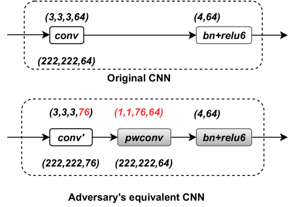
Figure 12: The equivalent CNN architecture needed to be trained by an adversary. The grey color marks the weights of the layers with unknown parameters that the adversary has to train. The weights shape is marked on top of the box and the output shape is marked under the box.

Illustration. In order to study the advantage an adversary might have in ShadownNet, over a black-box model stealing attack, we assume that the adversary reuses the transformed weights to build an equivalent CNN. Consider the example CNN from Figure 1 – the minimum equivalent CNN that reuses the transformed weights is shown in Figure 12. As mentioned before in Section IV-D, the linear transformation layer is essentially a pointwise convolutional layer and we use pwconv to represent it inside the TEE. Note that the mask/unmask layers are not needed to construct the equivalent CNN.

We use the number of learnable parameters to assess the difficulty of training a CNN. In our example, the block in the original CNN has $3\times 3\times 3\times 64+4\times 64=1,984$ parameters while the block in the adversary’s equivalent CNN has $76\times 64+4\times 64=5,120$ parameters to be trained. Here, $4\times 64$ learnable parameters are due to the batch normalization (bn) layer. There are $76$ kernels in the conv’ layer and this number can be configured via the obfuscation ratio, which is set to $r=1.2$ in our example ($76=64\times 1.2$). In fact, even for $r=1$, the minimum allowed value, the adversary’s CNN has more learnable parameters ($64\times 64+4\times 64=4,480$).

References

- [1] HiKey 960 . https://www.96boards.org/product/hikey960/.
- [2] Android 7.0 Compatibility Definition. https://source.android.com/docs/compatibility/7.0/android-7.0-cdd#9_11_keys_and_credentials.
- [3] AppLock Face/Voice Recognition - Apps on Google Play. https://play.google.com/store/apps/details?id=com.sensory.tsapplock\&hl=en_US\&gl=US.
- [4] Arm Compute Library. https://www.arm.com/why-arm/technologies/compute-library.
- [5] Arm TrustZone. https://developer.arm.com/ip-products/security-ip/trustzone.
- [6] Asylo, An open and flexible framework for enclave applications. https://asylo.dev/.
- [7] Card Scanner - Apps on Google Play. https://play.google.com/store/apps/details?id=com.zoho.android.cardscanner&hl=en_US&gl=US.
- [8] The cifar-100 dataset. https://www.cs.toronto.edu/~kriz/cifar.html.
- [9] Coral: An ecosystem for local AI. https://blog.tensorflow.org/2019/01/tensorflow-lite-now-faster-with-mobile.html.
- [10] Coral: An ecosystem for local AI. https://coral.ai/about-coral/.
- [11] Eigen. http://eigen.tuxfamily.org/index.php?title=Main_Page.
- [12] Fritz AI: Model Protection - Secure your Intellectual Property from being tampered-with or stolen. https://www.fritz.ai/features/model-protection.html.
- [13] Google Translate - Apps on Google Play. https://play.google.com/store/apps/details?id=com.google.android.apps.translate&hl=en_US&gl=US.
- [14] Minivgg pre-trained model. https://pyimagesearch.com/2021/05/22/minivggnet-going-deeper-with-cnns/.
- [15] Mobilenets pre-trained model. https://keras.io/api/applications/.
- [16] Model-extraction-iclr. https://github.com/cleverhans-lab/model-extraction-iclr.
- [17] OP-TEE AOSP support. https://optee.readthedocs.io/en/latest/building/aosp/aosp.html.
- [18] Optee-os issue : Keep the context of the last session. https://github.com/OP-TEE/optee_os/pull/4891/commits/0fa9b4efadf8ae7a48f87184660d6b6f8e56749d.
- [19] Optee-os issue :questions about memory management. https://github.com/OP-TEE/optee_os/issues/5042.
- [20] Resnet-404 pre-trained model. https://github.com/wikibook/keras/blob/master/chapter2-deep-networks/resnet-cifar10-2.2.1.py.
- [21] Resnet-44 pre-trained model. https://github.com/wikibook/keras/blob/master/chapter2-deep-networks/resnet-cifar10-2.2.1.py.
- [22] ShadowNet Repo. https://github.com/RiS3-Lab/ShadowNet.
- [23] Tensorflow lite. https://www.tensorflow.org/lite.
- [24] Text Scanner [OCR] - Apps on Google Play. https://play.google.com/store/apps/details?id=com.peace.TextScanner&hl=en_US&gl=US.
- [25] TF Encrypted. https://github.com/tf-encrypted/tf-encrypted.
- [26] TF Lite Android Image Classifier App Example. https://github.com/tensorflow/tensorflow/tree/r2.2/tensorflow/lite/java/demo.
- [27] TF Trusted. https://github.com/dropoutlabs/tf-trusted.
- [28] TrustZone for Cortex-A. https://www.arm.com/why-arm/technologies/trustzone-for-cortex-a.
- [29] TrustZone for Cortex-M. https://www.arm.com/why-arm/technologies/trustzone-for-cortex-m.
- [30] Wiki: Trusted Execution Environment. https://en.wikipedia.org/wiki/Trusted_execution_environment.
- [31] Yolov4-tiny pre-trained model. https://github.com/bubbliiiing/yolov4-tiny-keras.
- [32] Sebastian P Bayerl, Tommaso Frassetto, Patrick Jauernig, Korbinian Riedhammer, Ahmad-Reza Sadeghi, Thomas Schneider, Emmanuel Stapf, and Christian Weinert. Offline model guard: Secure and private ml on mobile devices. DATE 2020, 2020.
- [33] David Berthelot, Nicholas Carlini, Ian Goodfellow, Nicolas Papernot, Avital Oliver, and Colin A Raffel. Mixmatch: A holistic approach to semi-supervised learning. In H. Wallach, H. Larochelle, A. Beygelzimer, F. d'Alché-Buc, E. Fox, and R. Garnett, editors, Advances in Neural Information Processing Systems, volume 32. Curran Associates, Inc., 2019.
- [34] Alexey Bochkovskiy, Chien-Yao Wang, and Hong-Yuan Mark Liao. Yolov4: Optimal speed and accuracy of object detection. CoRR, abs/2004.10934, 2020.
- [35] Ferdinand Brasser, David Gens, Patrick Jauernig, Ahmad-Reza Sadeghi, and Emmanuel Stapf. Sanctuary: Arming trustzone with user-space enclaves. In NDSS, 2019.
- [36] Cristiano Breuel. Implementing Liveness Detection with Google ML Kit. https://towardsdatascience.com/implementing-liveness-detection-with-google-ml-kit-5e8c9f6dba45.
- [37] Xuhui Chen, Jinlong Ji, Lixing Yu, Changqing Luo, and Pan Li. Securenets: Secure inference of deep neural networks on an untrusted cloud. In Asian Conference on Machine Learning, pages 646–661, 2018.
- [38] Adam Dziedzic, Muhammad Ahmad Kaleem, Yu Shen Lu, and Nicolas Papernot. Increasing the cost of model extraction with calibrated proof of work. In ICLR (International Conference on Learning Representations) [SPOTLIGTH], 2022.
- [39] Mark Everingham, Luc Van Gool, Christopher KI Williams, John Winn, and Andrew Zisserman. The pascal visual object classes (voc) challenge. volume 88, pages 303–338. Springer, 2010.
- [40] Zahra Ghodsi, Tianyu Gu, and Siddharth Garg. Safetynets: Verifiable execution of deep neural networks on an untrusted cloud. In Advances in Neural Information Processing Systems, pages 4672–4681, 2017.
- [41] Ran Gilad-Bachrach, Nathan Dowlin, Kim Laine, Kristin Lauter, Michael Naehrig, and John Wernsing. Cryptonets: Applying neural networks to encrypted data with high throughput and accuracy. In International Conference on Machine Learning, pages 201–210, 2016.
- [42] Zhongshu Gu, Heqing Huang, Jialong Zhang, Dong Su, Ankita Lamba, Dimitrios Pendarakis, and Ian Molloy. Yerbabuena: Securing deep learning inference data via enclave-based ternary model partitioning. arXiv preprint arXiv:1807.00969, 2018.
- [43] Suyog Gupta, Ankur Agrawal, Kailash Gopalakrishnan, and Pritish Narayanan. Deep learning with limited numerical precision. In Proceedings of the 32nd International Conference on International Conference on Machine Learning - Volume 37, ICML’15, page 1737–1746. JMLR.org, 2015.
- [44] Lucjan Hanzlik, Yang Zhang, Kathrin Grosse, Ahmed Salem, Max Augustin, Michael Backes, and Mario Fritz. Mlcapsule: Guarded offline deployment of machine learning as a service. arXiv preprint arXiv:1808.00590, 2018.
- [45] Kaiming He, Xiangyu Zhang, Shaoqing Ren, and Jian Sun. Deep residual learning for image recognition. In Proceedings of the IEEE conference on computer vision and pattern recognition, pages 770–778, 2016.
- [46] Andrew G Howard, Menglong Zhu, Bo Chen, Dmitry Kalenichenko, Weijun Wang, Tobias Weyand, Marco Andreetto, and Hartwig Adam. Mobilenets: Efficient convolutional neural networks for mobile vision applications. arXiv preprint arXiv:1704.04861, 2017.
- [47] Matthew Jagielski, Nicholas Carlini, David Berthelot, Alex Kurakin, and Nicolas Papernot. High-fidelity extraction of neural network models. arXiv preprint arXiv:1909.01838, 2019.
- [48] Dongxu Ji, Qianying Zhang, Shijun Zhao, Zhiping Shi, and Yong Guan. Microtee: designing tee os based on the microkernel architecture. In 2019 18th IEEE International Conference On Trust, Security And Privacy In Computing And Communications/13th IEEE International Conference On Big Data Science And Engineering (TrustCom/BigDataSE), pages 26–33. IEEE, 2019.
- [49] Xiaoqian Jiang, Miran Kim, Kristin Lauter, and Yongsoo Song. Secure outsourced matrix computation and application to neural networks. In Proceedings of the 2018 ACM SIGSAC Conference on Computer and Communications Security, pages 1209–1222, 2018.
- [50] Chiraag Juvekar, Vinod Vaikuntanathan, and Anantha Chandrakasan. GAZELLE: A low latency framework for secure neural network inference. In 27th USENIX Security Symposium (USENIX Security 18), pages 1651–1669, 2018.
- [51] Jonathan Katz and Yehuda Lindell. Introduction to Modern Cryptography, Second Edition. Chapman & Hall/CRC, 2nd edition, 2014.
- [52] Alex Krizhevsky, Vinod Nair, and Geoffrey Hinton. Cifar-10 (canadian institute for advanced research).
- [53] Roland Kunkel, Do Le Quoc, Franz Gregor, Sergei Arnautov, Pramod Bhatotia, and Christof Fetzer. Tensorscone: A secure tensorflow framework using intel sgx. arXiv preprint arXiv:1902.04413, 2019.
- [54] Matthew Lentz, Rijurekha Sen, Peter Druschel, and Bobby Bhattacharjee. Secloak: Arm trustzone-based mobile peripheral control. In Proceedings of the 16th Annual International Conference on Mobile Systems, Applications, and Services, pages 1–13, 2018.
- [55] Linaro. Open Portable Trusted Execution Environment. https://www.op-tee.org/.
- [56] Fan Mo, Ali Shahin Shamsabadi, Kleomenis Katevas, Soteris Demetriou, Ilias Leontiadis, Andrea Cavallaro, and Hamed Haddadi. Darknetz: Towards model privacy at the edge using trusted execution environments. In ACM MobiSys 2020.
- [57] Tribhuvanesh Orekondy, Bernt Schiele, and Mario Fritz. Knockoff nets: Stealing functionality of black-box models. In 2019 IEEE/CVF Conference on Computer Vision and Pattern Recognition (CVPR), pages 4949–4958, 2019.
- [58] Keiron O’Shea and Ryan Nash. An introduction to convolutional neural networks. arXiv preprint arXiv:1511.08458, 2015.
- [59] Nicolas Papernot, Patrick McDaniel, Ian Goodfellow, Somesh Jha, Z Berkay Celik, and Ananthram Swami. Practical black-box attacks against machine learning. In Proceedings of the 2017 ACM on Asia conference on computer and communications security, pages 506–519, 2017.
- [60] Joseph Redmon. Darknet: Open source neural networks in c. http://pjreddie.com/darknet/, 2013–2016.
- [61] Joseph Redmon, Santosh Kumar Divvala, Ross B. Girshick, and Ali Farhadi. You only look once: Unified, real-time object detection. CoRR, abs/1506.02640, 2015.
- [62] M Sadegh Riazi, Christian Weinert, Oleksandr Tkachenko, Ebrahim M Songhori, Thomas Schneider, and Farinaz Koushanfar. Chameleon: A hybrid secure computation framework for machine learning applications. In Proceedings of the 2018 on Asia Conference on Computer and Communications Security, pages 707–721, 2018.
- [63] Frank Rubin. One-time pad cryptography. Cryptologia, 20(4):359–364, 1996.
- [64] Olga Russakovsky, Jia Deng, Hao Su, Jonathan Krause, Sanjeev Satheesh, Sean Ma, Zhiheng Huang, Andrej Karpathy, Aditya Khosla, Michael Bernstein, Alexander C. Berg, and Li Fei-Fei. ImageNet Large Scale Visual Recognition Challenge. International Journal of Computer Vision (IJCV), 115(3):211–252, 2015.
- [65] Sergio Salinas, Changqing Luo, Weixian Liao, and Pan Li. Efficient secure outsourcing of large-scale quadratic programs. In Proceedings of the 11th ACM on Asia Conference on Computer and Communications Security, pages 281–292, 2016.
- [66] Karen Simonyan and Andrew Zisserman. Very deep convolutional networks for large-scale image recognition. arXiv preprint arXiv:1409.1556, 2014.
- [67] Zhichuang Sun, Ruimin Sun, and Long Lu. Mind your weight (s): A large-scale study on insufficient machine learning model protection in mobile apps. arXiv preprint arXiv:2002.07687, 2020.
- [68] Christian Szegedy, Wei Liu, Yangqing Jia, Pierre Sermanet, Scott Reed, Dragomir Anguelov, Dumitru Erhan, Vincent Vanhoucke, and Andrew Rabinovich. Going deeper with convolutions. In Proceedings of the IEEE conference on computer vision and pattern recognition, pages 1–9, 2015.
- [69] Tianxiang Tan and Guohong Cao. Deep learning on mobile devices through neural processing units and edge computing. CoRR, abs/2112.02439, 2021.
- [70] Florian Tramer and Dan Boneh. Slalom: Fast, verifiable and private execution of neural networks in trusted hardware. arXiv preprint arXiv:1806.03287, 2018.
- [71] Florian Tramèr, Fan Zhang, Ari Juels, Michael K Reiter, and Thomas Ristenpart. Stealing machine learning models via prediction apis. In 25th USENIX Security Symposium (USENIX Security 16), pages 601–618, 2016.
- [72] Stavros Volos, Kapil Vaswani, and Rodrigo Bruno. Graviton: Trusted execution environments on gpus. In 13th USENIX Symposium on Operating Systems Design and Implementation (OSDI 18), pages 681–696, 2018.
- [73] Mengwei Xu, Jiawei Liu, Yuanqiang Liu, Felix Xiaozhu Lin, Yunxin Liu, and Xuanzhe Liu. A first look at deep learning apps on smartphones. In The World Wide Web Conference, pages 2125–2136, 2019.
- [74] Jason Yosinski, Jeff Clune, Yoshua Bengio, and Hod Lipson. How transferable are features in deep neural networks? In Advances in neural information processing systems, pages 3320–3328, 2014.
- [75] Yi Zhang, Jiun-Hao Liu, Chih-Yu Wang, and Hung-Yu Wei. Decomposable intelligence on cloud-edge iot framework for live video analytics. IEEE Internet of Things Journal, 7(9):8860–8873, 2020.