Optimal computation of anisotropic galaxy three point correlation function multipoles using 2DFFTLOG formalism

Abstract

We study two key issues militating against the use of the anisotropic three-point correlation function (3PCF) for cosmological parameter inference: difficulties with its computational estimation and high-dimensionality. We show how high-dimensionality may be reduced significantly by multipole decompositions of all angular dependence. This allows deriving the full expression for the multipole moments of the anisotropic 3PCF and its covariance matrix in a basis where the dimensionality reduces from nine to two at each multipole in the plane-parallel limit. We use 2D FFTLog formalism to show how the multipole moments with double momentum integrals over the product of bispectrum and two highly oscillating spherical Bessel functions and its covariance with double momentum integrals over the product of three galaxy power spectra and a combination of four highly oscillating spherical Bessel functions may be computed optimally.

1 Introduction

The three-point correlation function (3PCF) estimates the excess probability of finding three galaxies with locations at the vertices of a triangle. It provides an opportunity to probe information that cannot be obtained from the two-point correlation (2PCF), for example; measurement of the non-linear and tidal bias parameters [1]; probe of the early universe through measurement of various shapes of the primordial non-Gaussianity [2]; probe of the rate of growth of structure under non-linear gravitational evolution [3, 4];

The most fascinating use of the 3PCF of the large scale structure is as a probe of shapes of non-Gaussinty in the primordial density field predicted by the models of inflation and its alternatives [2, 5]. Models of inflation predict various shapes of the primordial bispectrum or the inflationary 3PCF [6]. A particular limit of these shapes act as a cosmological collider and could be used to probe the features of high energy particle interaction during inflation on energy scales that can never be achieved on earth [7]. The biggest obstacle in using the galaxy 3PCF to constrain these features is the huge computational overhead associated with computing different permutations of the triangle shapes on large scales and the dependence of galaxy 3PCF on many variables that make estimating the covariance matrix for cosmological inference a huge task.

The algorithm that counts triangles is generally not fast, especially on large scales where perturbations theory treatment is possible. In the homogenous and isotropic limit of 3PCF, Slepian & Eisenstein (2016) [8] proposed an algorithm that computes the multipole coefficients of the galaxy 3PCF without explicitly considering triplets of galaxies. The computation time scales like $\mathcal{O}(N^{2})$ against $\mathcal{O}(N^{3})$ in the traditional approach. This approach builds on the work of [9], who first introduced the idea. The key feature of this formalism involves decomposing the opening angle between any two sides of a triangle in Legendre polynomial

$$\zeta_{g}(r_{13},r_{23},\hat{\bm{r}}_{13}\cdot\hat{\bm{r}}_{23})=\sum_{\ell_{13}}\zeta_{g\ell_{13}}(r_{13},r_{23})\mathcal{L}_{\ell_{13}}(\hat{\bm{r}}_{13}\cdot\hat{\bm{r}}_{23})\,,$$ (1.1)

where $\mathcal{L}_{\ell_{13}}$ is the Legendre polynomial, $\zeta_{g\ell_{13}}$ is the multipole moments with respect to the angle between $\hat{\bm{r}}_{13}$ and $\hat{\bm{r}}_{23}$. This approach allows immediate insights into the information contained in all triangles by computing only the first few multipoles. The first detection of the BAO signal using the 3PCF relied on this approach [10]. Equation (1.1) is valid in real space, a minimal extension to the monopole of the redshift space bispectrum was done in [11]. The first attempt to extend equation (1.1) to account for anisotropy was given in [12, 13], where $\zeta_{g}$ is decomposed in spherical harmonics basis as

$$\zeta_{g}({\bm{r}}_{13},{\bm{r}}_{23})=\sum_{\ell_{1}m_{1}}\sum_{\ell_{2}m_{2}}\zeta_{g\ell_{1}\ell_{2}}^{m_{1}m_{2}}(r_{13},r_{23})Y_{\ell_{1}m_{1}}({\hat{\bm{r}}_{13}})Y^{\star}_{\ell_{2}m_{2}}({\hat{\bm{r}}_{23}})\,,$$ (1.2)

where $Y_{\ell m}$ is the spherical harmonics and $Y^{\star}_{\ell m}$ is the conjugate. The anisotropic 3PCF in equation (1.2) depends on two triangle sides $r_{13}$ and $r_{23}$, the angle each side of the triangle makes with the line of sight. Although equation (1.2) provides a complete spherical harmonics basis for decomposing the 3PCF into multipole moments, it does not correspond to the multipole moments of the redshift space galaxy bispectrum in the well-known Scoccimarro basis [14, 15, 16]. Recently [17] use a tri-polar spherical harmonics to decompose $\zeta_{g}$ in spherical harmonics

$$\zeta_{g}({\bm{r}}_{13},{\bm{r}}_{23},{{\bf\hat{n}}}) = \sum_{\ell_{1}+\ell_{2}+L={\rm even}}\zeta_{g\ell_{1}\ell_{2}L}({r}_{13},{r}_{23})\,S_{\ell_{1}\ell_{2}L}(\hat{\bm{r}}_{13},\hat{\bm{r}}_{23},{{\bf\hat{n}}}),$$ (1.3)

where $S_{\ell_{1}\ell_{2}L}$ is a Tri-polar spherical harmonics [18] and the index $L$ is associated with an average over all directions ${{\bf\hat{n}}}$ and in Scoccimarro basis corresponds to the multipole moments of the redshift space bispectrum. The index $\ell_{1}$ and $\ell_{2}$ have no obvious physical meaning and there is no guidance on the maximum order of the spherical harmonics to sum in order to recover all the signal.

Our target here is to show for the first time how to extend the formalism introduced in [9] (equation (1.1)) to anisotropic galaxy 3PCF. Then use the extended formalism to derive the multipole moments of the anisotropic galaxy 3PCF in a basis that corresponds to the Scoccimarro basis for the galaxy bispectrum in redshift-space [14]. In Scoccimarro basis, one starts with nine parameters that describe each coordinate of the three triangle vertices, then impose translation invariance, which reduces the nine parameters to six. Imposing the rotation invariance about the line of sight reduces it further to five: three parameters characterise the triangle’s shape, e.g. two sides and the enclosed angle, and the remaining two describe the orientation of the triangle with respect to the line of sight. It is possible to further reduce the dimensionality to four by averaging over azimuthal degree of freedom. This allows to decompose the resulting anisotropic 3PCF in Legendre polynomials with the angle between the line of sight and one side of the triangle and the angle between any two sides of the triangle as arguments.

Furthermore, we show how to optimally compute the double momentum integrals over the product of the galaxy bispectrum and two spherical Bessel functions that appear in the expression of the multipole moments of the anisotropic 3PCF using the 2D FFTLog formalism introduced in [19]. This formalism allows to expand the dependence on the wave number in a series of power laws sampled in log-log space. The power laws expansion allows to perform the integral over the spherical Bessel function analytically in terms of the Gamma functions for the multipoles of the 3PCF and in terms of the the hypergeometric function for its covariance matrix.

We hope that the tools discussed here would be useful in extending the cosmological analysis of Baryon Acoustic Oscillation (BAO) with data from the extended Baryon Oscillation Spectroscopic Survey (eBOSS) beyond the 2PCF [22, 23, 24]. Also, the approach we discuss here would be beneficial to the analysis of data from future spectroscopic surveys such as EUCLID [25], DESI [26], SKA [27] etc.

The rest of the paper is structured as follows: we review the derivation of the multipole moments of 3PCF in real space in section 2.1 and derive the corresponding expression for the anisotropic 3PCF in sub-section 2.2. The comparison between our expression for the multipole moments of 3PCF and previous studies is given in section 2.3. We derive the covariance matrix of the estimator of the multipole moments of the 3PCF in section 3 and conclude in section 4. We provide details on the implementation of the 2D FFTLog formalism for computing the anisotropic 3PCF in Appendix A and for the covariance matrix of the multipole moments in Appendix B . We give details on the derivation of the galaxy bispectrum in Appendix C and further technical detail on the multipole decomposition is given in Appendix D.

Notations: We consider a universe which consists of dark matter and the cosmological constant only, i.e. we ignore the effects of radiation and anisotropic stress tensor. The perturbation theory expansion of any quantity $X$ is normalized as follows: $X=\bar{X}+X^{\text{\tiny\color[rgb]{1,0,0}{({1}})}}+X^{\text{\tiny\color[rgb]{0,1,0}{({2}})}}/2,$ where $\bar{X}$ denotes the FLRW background component. $X^{\text{\tiny\color[rgb]{1,0,0}{({1}})}}$ and $X^{\text{\tiny\color[rgb]{0,1,0}{({2}})}}$ are first and second order parts respectively. We adopt the following values for the cosmological parameters of the standard model [28, 29]: Hubble parameter, $h=0.674$, baryon density parameter, $\Omega_{b}=0.0493$, dark matter density parameter, $\Omega_{\rm{cdm}}=0.264$, matter density parameter, $\Omega_{m}=\Omega_{\rm{cdm}}+\Omega_{b}$, spectral index, $n_{s}=0.9608$, and the amplitude of the primordial perturbation, $A_{s}=2.198\times 10^{9}$.

2 Galaxy three-point correlation function

In this section, we introduced our notations and the basic ingredients of our approach by reviewing the formalism introduced in [9] for the isotropic 3PCF before proceeding to the anisotropic case.

2.1 Real space galaxy three-point correlation function

The number of galaxies, $N$, within a given patch of the sky, ${\rm{d}}\Omega$, at a given redshift slice, ${\rm{d}}z$ is given by [30, 31, 32]

$$\frac{{\rm{dN}}}{\rm{d}z{\rm{d}}\Omega}=\bar{n}_{g}({z})\left[1+\delta_{g}({\bm{r}})\right]{d}_{A}^{2}\frac{\rm{d}\chi}{\rm{d}z},$$ (2.1)

where $\chi$ is the comoving distance to the source, $d_{A}$ is the area distance and $\bar{n}_{g}$ is the mean proper number density of galaxies. The galaxy density fluctuation $\delta_{g}$ is related to the matter density fluctuation $\delta_{m}$ according to the Eulerian bias model [33, 34]

$$\delta_{\rm{g}}({\bm{r}})=b_{1}\delta_{m}({\bm{r}})+\frac{1}{2}\left[b_{2}\delta_{\rm{m}}({\bm{r}}))^{2}+b_{\mathcal{K}^{2}}\mathcal{K}^{2}({\bm{r}})\right]\,,$$ (2.2)

where $\mathcal{K}^{2}=\mathcal{K}_{ij}\mathcal{K}^{ij}$ is the scalar invariant of the tidal tensor:

$$\mathcal{K}_{ij}({\bm{r}})=\left(\frac{2}{3\Omega_{m}\mathcal{H}}\right)\left[\partial_{i}\partial_{j}\Phi({\bm{r}})-\frac{1}{3}\nabla^{2}\Phi\right]({\bm{r}})\,,$$

$\Phi$ is the gravitational potential, it is related to $\delta_{m}$ through the Poisson equation $\delta_{m}=(2/3\Omega_{m}\mathcal{H})\nabla^{2}\Phi$, where $\mathcal{H}$ is the conformal Hubble rate. Here, $b_{1}$, $b_{2}$ and $b_{\mathcal{K}^{2}}$ are the linear, non-linear and tidal bias parameters respectively. Without loss of generality, we focus on the clustering bias parameters for a typical Stage IV spectroscopic survey H$\alpha$ emission line survey [35]

$$b_{1}\left(z\right) = 0.9+0.4z\,,$$ (2.3)

$$b_{2}\left(z\right) = -0.704172-0.207993z+0.183023z^{2}-0.00771288z^{3}\,,$$ (2.4)

$$b_{\mathcal{K}^{2}}\left(z\right) = -\frac{4}{7}(b_{1}(z)-1)$$ (2.5)

The galaxy 3PCF in configuration space, $\zeta_{g}$, is defined as the ensemble average of the galaxy density contrast measured at three different points on the sky

$$\zeta_{g}({\bm{r}}_{1},{\bm{r}}_{2},{\bm{r}}_{3}) \equiv \langle\delta_{g}({\bm{r}}_{1})\delta_{g}({\bm{r}}_{2})\delta_{g}({\bm{r}}_{3})\rangle\,,$$ (2.6)

$$= \int\frac{{d}^{3}k_{1}}{(2\pi)^{3}}\int\frac{{d}^{2}k_{2}}{(2\pi)^{3}}\int\frac{{d}^{3}k_{3}}{(2\pi)^{3}}e^{i{\bm{k}}_{1}\cdot{\bm{r}}_{1}+i{\bm{k}}_{2}\cdot{\bm{r}}_{2}+i{\bm{k}}_{3}\cdot{\bm{r}}_{3}}B_{g}({\bm{k}}_{1},{\bm{k}}_{2},{\bm{k}}_{3})\delta^{D}\left({\bm{k}}_{1}+{\bm{k}}_{2}+{\bm{k}}_{3}\right)\,,\qquad$$ (2.7)

where we have expanded $\delta_{g}$ in Fourier space and introduced the galaxy bispectrum $B_{g}$ (for more details on the definition of the galaxy bispectrum see equation (C.8) in Appendix C). The key point to note is that the definition of $B_{g}$ includes the full cyclic permutation of the galaxy density $\delta_{g}({\bm{k}})$ over the three vertices of a triangle:

$$B_{g}(\bm{k}_{1},\bm{k}_{2},\bm{k}_{3})=B^{123}_{g}(\bm{k}_{1},\bm{k}_{2},\bm{k}_{3})+B^{231}_{g}(\bm{k}_{2},\bm{k}_{3},\bm{k}_{1})+B^{312}_{g}(\bm{k}_{3},\bm{k}_{1},\bm{k}_{2})\,.$$ (2.8)

where the superscript on each $B_{g}$ indicates the corresponding cyclic permutations of the ${\bm{k}}$ indices. The ${\bm{k}}^{\prime}s$ are vectors in Fourier space, its magnitude is related to the wavelength of mode of the density perturbations, $\delta^{D}$ is the Dirac delta function which enforces the closure property on the triangle formed by three Fourier space vectors. $\zeta_{g}$ depends on three coordinates (i.e 9 free variables), imposing the translation invariance reduces to 6 free parameters:

$$\zeta_{g}({\bm{r}}_{13},{\bm{r}}_{23}) = \int\frac{{d}^{3}k_{1}}{(2\pi)^{3}}\int\frac{{d}^{3}k_{2}}{(2\pi)^{3}}B_{g}({\bm{k}}_{1},{\bm{k}}_{2},-{\bm{k}}_{1}-{\bm{k}}_{2})e^{i{\bm{k}}_{1}\cdot{\bm{r}}_{13}+i{\bm{k}}_{2}\cdot{\bm{r}}_{23}}\,.$$ (2.9)

where we introduced a relative distance vector as ${\bm{r}}_{MN}={\bm{r}}_{M}-{\bm{r}}_{N}$, $M,N$ runs from $1\cdots 3$. The vectors ${\bm{r}}_{MN}$ form sides of a closed triangle in real space, it satisfies the closure relation: ${\bm{r}}_{12}+{\bm{r}}_{23}+{\bm{r}}_{31}=0$. Using the closure property, we reduce the number of free variables from 6 to 3, i.e two side lengths and one enclosed angle $r_{13}$, $r_{23}$ and $\hat{\bm{r}}_{13}\cdot\hat{\bm{r}}_{23}$, where $\nu_{13}=\hat{\bm{r}}_{13}\cdot\hat{\bm{r}}_{23}$ is the angle between ${\bm{r}}_{13}$ and ${\bm{r}}_{23}$. In the plane wave expansion, we can expand $e^{i{\bm{k}}\cdot{\bm{r}}_{MN}}$ in Legendre polynomial

$$e^{i{\bm{k}}\cdot{\bm{r}}_{MN}}=\sum_{\ell}(2\ell+1)i^{\ell}j_{\ell}(kr_{MN})\mathcal{L}_{\ell}(\hat{\bf{r}}_{MN}\cdot\hat{{\bm{k}}})\,,$$ (2.10)

where $\mathcal{L}_{\ell}$ is the Legendre polynomial of order $\ell$ and $j_{\ell}$ is the spherical Bessel function. Again, $B_{g}$ is the real space galaxy bispectrum, it depends on two amplitudes $k_{1}$, $k_{2}$ and the angle between them $\mu_{12}=\hat{\bm{k}}_{1}\cdot\hat{\bm{k}}_{2}$. We expand $\mu_{12}$ and $\nu_{13}$ in Legendre polynomial: $B_{g}({k}_{1},{k}_{2},\mu_{12})=\sum_{\ell_{12}}B_{g\ell_{12}}({k}_{1},{k}_{2})\mathcal{L}_{\ell_{12}}(\mu_{12})\,$ and $\zeta_{g}^{123}({r}_{13},{r}_{23},\nu_{13})=\sum_{\ell_{13}}\zeta_{g\ell_{13}}({r}_{31},{r}_{23})\mathcal{L}_{\ell_{13}}(\nu_{13})$ respectively. Using the orthogonality relation we obtain the real space 3PCF  [9, 36, 11]

$$\zeta_{g\ell_{12}}({r}_{31},{r}_{23}) = {(-1)^{\ell_{12}}}\int\frac{{d}k_{1}k^{2}_{1}}{2\pi^{2}}\int\frac{{d}k_{2}k^{2}_{2}}{2\pi^{2}}B_{{g}\ell_{12}}(k_{1},k_{2})j_{\ell_{12}}(k_{1}r_{31})j_{\ell_{12}}(k_{2}r_{23})\,.$$ (2.11)

At a given $\ell_{12}$, $\zeta_{g\ell_{12}}$ depends only on ${r}_{31},$ and ${r}_{23}$.

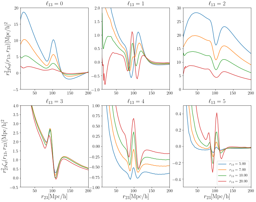
Figure 1: We show the first few shape multipoles of the real space 3PCF for the H$\alpha$ emission line galaxy. We fixed one side of the triangle to $r_{13}=5,7,10,20~{}[h^{-1}\rm{Mpc}]=$[blue, yellow, green, red] at $z=1.0$. The monopole and the quadrupole moments have the highest amplitude. The BAO features appear on all the multipoles.

The numerical computation of equation (2.11) has been intractable using traditional methods like the Quadrature. This is because of the double integral over a product of the galaxy bispectrum and highly oscillating product of two spherical Bessel functions. This constraint motivated earlier works to focus on the separable limit where double integrals could be reduced to two independent 1D integrals over a single spherical Bessel function before the cyclic permutation of the bispectrum given in equation (2.8) is taken. This approach which was initiated in [14] is based on the realisation that in real space, the galaxy bispectrum is separable before cyclic permutation is taken. This leads to the concept of ‘pre-cyclic permutation’ 3PCF:

$${\zeta}_{g0}^{123}({r}_{31},{r}_{23}) = \left[2b_{1}^{2}b_{2}+\frac{34}{21}b_{1}^{3}\right]\xi_{0}(r_{31})\xi_{0}(r_{23})\,,$$ (2.12)

$${\zeta}_{g1}^{123}({r}_{31},{r}_{23}) = -2b_{1}^{3}\left[\xi_{1}^{[-1]}(r_{31})\xi_{1}^{[+1]}(r_{31})+\xi_{1}^{[-1]}(r_{23})\xi_{1}^{[+1]}(r_{23})\right]\,,$$ (2.13)

$${\zeta}^{123}_{g2}({r}_{31},{r}_{23}) = \left[\frac{8}{21}b_{1}^{3}+\frac{2}{3}{b_{\mathcal{K}^{2}}}b_{1}^{2}\right]\xi_{2}(r_{31})\xi_{2}(r_{23})\,,$$ (2.14)

where ${\zeta}_{g\ell}^{123}$ denotes the 3PCF corresponding to the first cyclic permutation of the bispectrum defined in equation (2.8). The double momentum integral has now reduced to separate 1D integrals which can easily be performed using the traditional quadrature methods

$$\xi_{\ell}(r_{MN})=\int\frac{{d}kk^{2}}{2\pi^{2}}{P_{m}(k)}j_{\ell}(kr_{MN})\,,\qquad\xi_{\ell}^{[\pm 1]}(r_{MN})=\int\frac{{d}k\,k^{2}k^{\pm 1}}{2\pi^{2}}{P_{m}(k)}j_{\ell}(kr_{MN})\,.$$ (2.15)

The multipole moments of the full 3PCF are then obtained by taking the cyclic permutations operations done in real space

$${\zeta}_{\ell_{12}}({r}_{12},{r}_{23}) = \frac{(2\ell_{12}+1)}{2}\int_{-1}^{1}{d}\nu_{13}\bigg{[}\sum_{L_{12}}{\zeta}_{gL_{12}}^{312}({r}_{12},{r}_{23})\mathcal{L}_{L_{12}}({\hat{\bm{r}}_{12}}\cdot{\hat{\bm{r}}_{23}})$$

$$+\sum_{L_{23}}{\zeta}_{gL_{23}}^{231}({r}_{12},{r}_{31})\mathcal{L}_{L_{23}}({\hat{\bm{r}}_{12}}\cdot{\hat{\bm{r}}_{31}})+\sum_{L_{31}}{\zeta}_{gL_{31}}^{123}({r}_{23},{r}_{31})\mathcal{L}_{\ell_{31}}({\hat{\bm{r}}_{23}}\cdot{\hat{\bm{r}}_{31}})\bigg{]}\mathcal{L}_{\ell_{12}}({\hat{\bm{r}}_{13}}\cdot{\hat{\bm{r}}_{23}})\,.$$

where the cosine rule may be used to express ${\hat{\bm{r}}_{12}}\cdot{\hat{\bm{r}}_{23}}$ and ${\hat{\bm{r}}_{23}}\cdot{\hat{\bm{r}}_{31}}$ in terms of $({\hat{\bm{r}}_{13}}\cdot{\hat{\bm{r}}_{23}})$. Extension of this approach to the isotropic limit of the anisotropic 3PCF leads to a complicated results [11]. This is because of the angular dependence of the second order redshift space distortion term which involves a $k_{3}$ wave vector which weakens the separability argument.

Our approach avoids this bottleneck by performing the integration in equation (2.11) using 2D FFTLog. The 2D FFTLog formalism was introduced in [19], where it was used to perform the 2D integral that appears in the expression for the non-Gaussian covariance matrix of the two point correlation function (2PCF). We have adapted this for the 3PCF. We described in detail how this works in Appendix A. Essentially, it involves decomposing the multipoles of the dimensionless galaxy bispectrum ${\Delta^{\rm{Real}}_{\rm{B}\ell_{12}}(k_{1},k_{2})={k_{1}^{3}k_{2}^{3}B_{g\ell_{12}}(k_{1},k_{2})}/{(2\pi^{2})^{2}}}$  in a finite number of power laws sampled in log-log space. Although the double integrals in equation (2.11) run from zero to infinity, use the fact that the integral converges at a finite $k_{\rm{max}}$ to write

$$\zeta_{g\ell_{12}}({r}_{13},{r}_{23}) = i^{2\ell_{12}}\int_{k_{\rm{min}}}^{k_{\rm{max}}}\frac{{d}k_{1}}{k_{1}}\int_{k_{\rm{min}}}^{k_{\rm{max}}}\frac{{d}k_{2}}{k_{2}}{\Delta^{\rm{Real}}_{{\rm{B}}\ell_{12}}}(k_{1},k_{2})j_{\ell_{12}}(k_{1}r_{13})j_{\ell_{12}}(k_{2}r_{23})\,,$$ (2.17)

where we set the $k$-limits to $[k_{\rm{min}},k_{\rm{max}}]\propto[10^{-4},2.0]$ [h/Mpc]. Note that the bispectrum has wiggles in $k$ due to the Baryon Acoustic oscillation (BAO), therefore, care must be taken when choosing $k_{\rm{min}}$ and $k_{\rm{max}}$ such that the k-range covers scales that contain these features. We show in Figure 1 the first six multipoles of the 3PCF in real space. We find strong BAO features in all the multipoles considered. For $\ell_{12}=0$ and one side of the triangle kept short, for example $r_{13}\sim$ short, the amplitude of the monopole becomes negative on large scales. Note that the contribution of the shape quadrupole moment is greater than that the shape monopole moment at say $r_{13}=5~{}[h^{-1}\rm{Mpc}]$ in Figure 1. This is due to the bias parameters of the H$\alpha$ emission line galaxy we are considering. For this tracer, the nonlinear bias parameter is negative, see equation (2.4), this reduces the amplitude of the monopole moment as can be seen in equation (2.12). The nonlinear bias parameter does not appear in the expression for the shape quadrupole moment, see equation (2.14). The heat map exploring the entire parameter space of $r_{13}$ and $r_{23}$ is given in Figure 5.

Finally, we compare the performance of the 2D FFTLog integration to the numerical integration using 2D Simpson’s rule implementation of equation (2.17). The comparisons were done with Python 3.7 running on MacBook Pro with 2.3 GHz Dual-Core Intel Core i5 processor. We consider just a single shape of the 3PCF with $r_{13}=5~{}[h^{-1}\rm{Mpc}]$ at the redshift of one ($z=1.0)$. It took more than two weeks with 6500 sub-divisions of $[k_{\rm{min}},k_{\rm{max}}]$ for both $k_{1}$ and $k_{2}$ to obtain the results shown in Figure 2. In general, there is less than 5% fractional difference between the two results for separation $20\leq r_{23}\leq 120~{}[h^{-1}\rm{Mpc}]$ except for the monopole and $\ell_{13}=5$. In the case of the monopole, we find that the fractional difference between the two approaches tends to decrease as we increase the number of sub-divisions but it takes even longer time to complete, hence we stopped at 6500 sub-divisions.

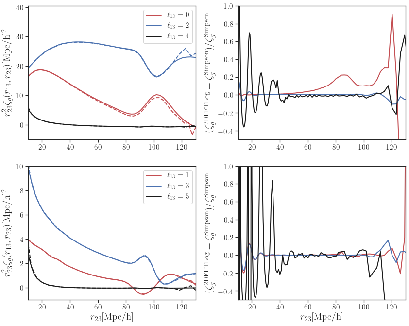
Figure 2: We compare the results of integration of equation (2.17) using 2D FFTLog to numeral integration using 2D Simpson’s rule implementation in python 3.7. The thicks lines denotes the result from 2D FFTLog implementation while the dash line corresponds to 2D Simpson’s rule. In both cases, we set $r_{13}=5~{}[h^{-1}\rm{Mpc}]$ and redshift at $z=1.0$.

2.2 Redshift space galaxy three-point correlation function

In redshift space, an observer infers the galaxy position, ${\bf{s}}_{\rm{\tiny{obs}}}$, at a slightly displaced position from the physical position of the galaxy, ${{\bm{r}}}$, due to the effect of the peculiar velocity according to

$${\bm{s}}_{\rm{\tiny{obs}}} = {{\bm{r}}}-\frac{1}{\mathcal{H}}{{\partial_{{}_{{\text{\tiny$\|$}}}}v}}\,{{\bf\hat{n}}}+\mathcal{O}(\epsilon)^{2}\,,$$ (2.18)

where ${{\bf\hat{n}}}$ is the Line of Sight (LoS) direction, ${{v^{i}}}=\partial^{i}v$ is the peculiar velocity of the source and $\epsilon$ is a small parameter that controls our perturbative expansion with respect to the background spacetime. Substituting equation (2.18) in equation (2.1), the number count fluctuations becomes:

$${\Delta_{g}}(z,{{\bf\hat{n}}}) = \delta_{g}-\frac{1}{\mathcal{H}}\partial_{\|}^{2}v-\frac{2}{\mathcal{H}}\bigg{[}\delta_{g}\partial_{\parallel}^{2}v+\partial_{\parallel}v\partial_{\parallel}\delta_{g}\bigg{]}+\frac{2}{\mathcal{H}^{2}}\bigg{[}\left(\partial_{\parallel}^{2}v\right)^{2}+\partial_{\parallel}v\partial_{\parallel}^{3}v\bigg{]}\,.$$ (2.19)

This is a leading order approximation, the full expression is given in [37, 38, 39]. We neglected the weak gravitational lensing terms that contribute at the same order as the terms in equation (2.19) since we are interested in the Plane-Parallel limit [40, 41]. Given equation (2.19), the 3PCF in redshift space is given by

$${\zeta^{\rm{RSD}}_{g}({\bm{r}}_{13},{\bm{r}}_{23},{{\bf\hat{n}}})} = \sum_{\ell_{1},\ell_{2}=0}^{\ell_{\text{max}}}{(2\ell_{1}+1)(2\ell_{2}+1)}\int\frac{{d}k_{1}k^{2}_{1}}{(2\pi)^{3}}\int\frac{{d}k_{2}k^{2}_{2}}{(2\pi)^{3}}i^{\ell_{1}+\ell_{2}}\int{d}{\bm{k}}_{{\bot}_{1}}\int{d}{\bm{k}}_{{\bot}_{2}}$$ (2.20)

$$\times B_{{g}}({\bm{k}}_{1},{\bm{k}}_{2},{{\bf\hat{n}}})j_{\ell_{1}}(k_{1}r_{13})j_{\ell_{2}}(k_{2}r_{23})\mathcal{L}_{\ell_{1}}({\hat{\bm{r}}}_{13}\cdot{\hat{\bm{k}}}_{1})\mathcal{L}_{\ell_{2}}({\hat{\bm{r}}}_{23}\cdot{\hat{\bm{k}}}_{2})\,,$$

where we have performed the delta function integral which enforces the closure relation for triangles and decomposed the angles ${\bm{r}}_{13}\cdot{\bm{k}}_{1}$ and ${\bm{r}}_{23}\cdot{\bm{k}}_{2}$ in plane-wave. $\zeta_{g}^{\rm{RSD}}({\bm{r}}_{13},{\bm{r}}_{23},{{\bf\hat{n}}})$ depends on six free parameters in plane parallel limit. Using the closure property and rotation with respect to the LoS direction, we can express $\nu_{2}={{\bf\hat{n}}}\cdot{\bm{r}}_{13}$ and $\nu_{3}={{\bf\hat{n}}}\cdot{\bm{r}}_{23}$ in terms of $\nu_{1}$ and $\phi_{n}$ [42]

$$\nu_{2} = \nu_{1}\nu_{13}+\sqrt{1-\nu_{1}^{2}}\sqrt{1-\nu^{2}_{13}}\cos\phi_{n}\,,$$ (2.21)

$$\nu_{3} = -\frac{r_{13}}{r_{12}}\nu_{1}-\frac{r_{23}}{r_{12}}\nu_{2}\,,$$ (2.22)

where $\cos(\nu_{13})={\bm{r}}_{13}\cdot{\bm{r}}_{23}/(r_{13}r_{23})$ is the cosine of the angle between ${\bm{r}}_{13}$ and ${\bm{r}}_{23}$ and $\phi_{n}$ is the azimuthal angle that describes the orientation of the triangle with respect to the LoS. This is a configuration space version of the Scoccimarro basis [43, 15]. At the moment, there are five free parameters that describe $\zeta_{g}({r}_{13},{r}_{23},\nu_{13},{\nu}_{1},\phi_{n})$. We can reduce it further to four by averaging over the azimuthal angle leading to the $\phi_{n}$-average 3PCF or azimuthal angle average 3PCF

$$\zeta_{g}^{\phi_{n}}({r}_{13},{r}_{23},\nu_{13},\nu_{1})=\int_{0}^{2\pi}\frac{{d}\phi_{n}}{2\pi}\zeta_{g}({r}_{13},{r}_{23},\nu_{13},\nu_{1},{\phi_{n}})\,.$$ (2.23)

It is already well-known that the $\phi_{n}$-averaged galaxy bispectrum are computationally less demanding to estimate given a galaxy catalogue [44, 15]. This is due to the reduction in dimensionality. Also, this limit helps to improve the signal to noise ratio [2] and there is a negligible information loss [45]. At this point, we can now expand the $\phi_{n}$-averaged 3PCF in Legendre polynomial: $\zeta_{g}^{\phi_{n}}({r}_{13},{r}_{23},\nu_{13},\nu_{1})=\sum_{\ell_{13}}\sum_{L}\zeta_{gL\ell_{13}}^{\phi_{n}}({r}_{13},{r}_{23})\mathcal{L}_{\ell_{13}}(\nu_{13})\mathcal{L}_{L}(\nu_{1})\,.$ Similarly, we define the $\phi_{n}$-averaged galaxy bispectrum

$$B_{g}^{\phi_{n}}({k}_{1},{k}_{2},\mu_{12},\mu_{1})\equiv\int_{0}^{2\pi}\frac{{d}\phi_{n}}{2\pi}B_{g}({k}_{1},{k}_{2},\mu_{12},\mu_{1},\phi_{n})\,$$ (2.24)

and we expand the enclosed angle in Fourier space in Legendre polynomial $B_{g}^{\phi_{n}}({k}_{1},{k}_{2},\mu_{12},\mu_{1})=\sum_{L=0}^{\infty}\sum_{\ell_{12}}B^{\phi_{n}}_{gL\ell_{12}}({k}_{1},{k}_{2})\mathcal{L}_{\ell_{12}}(\hat{\bm{k}}_{1}\cdot\hat{\bm{k}}_{2})\mathcal{L}_{L}({\hat{\bm{k}}}_{1}\cdot{{\bf\hat{n}}})\,.$ The multipoles of $B_{g}^{\phi_{n}}$ is obtained using the orthogonality condition for the Legendre polynomial

$$B^{\phi_{n}}_{gL\ell_{12}}({k}_{1},{k}_{2}) = {{(2L+1)\over 2}}\frac{(2\ell_{12}+1)}{2}\int_{-1}^{1}{d}\mu_{12}\int_{-1}^{1}{d}\mu_{1}\,B_{g}^{\phi_{n}}({k}_{1},{k}_{2},\mu_{12},\mu_{1})$$

$$\times{\cal{L}}_{L}(\mu_{1})\mathcal{L}_{\ell_{12}}(\mu_{12})\,.$$

Similarly, we obtain the multipole moments $\zeta^{\phi_{n}}_{gL\ell_{13}}$ by decomposing $\mathcal{L}_{L}$ and $\mathcal{L}_{\ell_{13}}$ into spherical harmonics, then using the convolution theorem of spherical harmonics and the orthonormality relation we find

$$\zeta^{\phi_{n}}_{gL\ell_{13}}({r}_{13},{r}_{23}) = \frac{(2L+1)(2\ell_{13}+1)}{(4\pi)^{2}\mathcal{H}_{\ell_{13},L,\ell_{3}}}\int{d^{2}\hat{\bm{r}}_{13}}\int{d^{2}\hat{\bm{r}}_{23}}\int{d^{2}\hat{n}}$$ (2.29)

$$\times\sum_{m_{13}Mm_{3}}\left({\begin{array}[]{ccc}\ell_{13}&L&\ell_{3}\\ m_{13}&{M}&m_{3}\\ \end{array}}\right)Y_{\ell_{3}m_{3}}({\bm{r}}_{13})Y^{\ast}_{\ell_{13}m_{13}}({\bm{r}}_{23})Y^{\ast}_{LM}({{\bf\hat{n}}})\zeta_{g}^{\phi_{n}}({r}_{13},{r}_{23},\nu_{13},\nu_{1})\,,$$

where $Y_{\ell m}$ is the spherical harmonics, the bracket is the Wigner $3j$ symbol, it satisfies the triangular condition, i.e it is zero unless all these conditions are satisfied $|\ell_{13}-L|\leq\ell_{3}\leq\ell_{13}+L$ and $m_{13}+M+m_{3}=0$. We have introduced $\mathcal{H}_{\ell_{1}\ell_{2}\ell_{3}}^{0,0,0}$

$$\mathcal{H}_{\ell_{1}\ell_{2}\ell_{3}}^{0,0,0} = \sqrt{\frac{(2\ell_{1}+1)(2\ell_{2}+1)(2\ell_{3}+1)}{4\pi}}\begin{pmatrix}\ell_{1}&\ell_{2}&\ell_{3}\\ 0&0&0\end{pmatrix}\,.$$ (2.30)

Putting the multipole moment of the galaxy bispectrum in equation (2.20) and then in equation (2.29) and performing the following $\hat{\bm{r}}_{13}$, $\hat{\bm{r}}_{23}$ and ${{\bf\hat{n}}}$ angular integrals we find

$${\zeta}^{\phi_{n}}_{L\ell_{12}}({r}_{13},{r}_{23}) = i^{\ell_{3}+\ell_{12}}\int_{0}^{\infty}\frac{{d}k_{1}k^{2}_{1}}{2\pi^{2}}\int_{0}^{\infty}\frac{{d}k_{2}k^{2}_{2}}{2\pi^{2}}B_{{g}L\ell_{12}}(k_{1},k_{2})j_{\ell_{3}}(k_{1}r_{13})j_{\ell_{12}}(k_{2}r_{23})\,.$$ (2.31)

Again ${\zeta}^{\phi_{n}}_{L\ell_{12}}$ is non-zero only when $|\ell_{12}-L|\leq\ell_{3}\leq\ell_{12}+L$. Some of the tools used to simplify the algebraic steps that lead to equation (2.31) are given in Appendix C. Choosing the value of $\ell_{3}$ that saturates the upper bound leads to

$$\zeta^{\phi_{n}}_{gL\ell_{12}}({r}_{13},{r}_{23}) = i^{2\ell_{12}+L}\int_{0}^{\infty}\frac{{d}k_{1}}{k_{1}}\int_{0}^{\infty}\frac{{d}k_{2}}{k_{2}}\Delta^{\rm{RSD}}_{{\rm{B}}L\ell_{12}}(k_{1},k_{2})j_{\ell_{12}+L}(k_{1}r_{13})j_{\ell_{12}}(k_{2}r_{23})\,,$$ (2.32)

where $\Delta^{\rm{RSD}}_{{\rm{B}}L\ell_{12}}(k_{1},k_{2})\equiv{{k_{1}^{3}k_{2}^{3}}B^{\phi_{n}}_{{g}L\ell_{12}}(k_{1},k_{2})}/{(2\pi^{2})^{2}}$ is the dimensionless galaxy bispectrum in redshift space. We recover exactly the real space 3PCF (equation (2.11)) in the isotropic limit $L=0$ and it agrees with [9].

We describe in detail how equation (2.32) is calculated numerically using the 2D FFTLog formalism in Appendix A. The multipole moments of the anisotropic 3PCF obtained by integrating equation (2.32) for the H$\alpha$ emission line galaxy is shown in Figure 3.

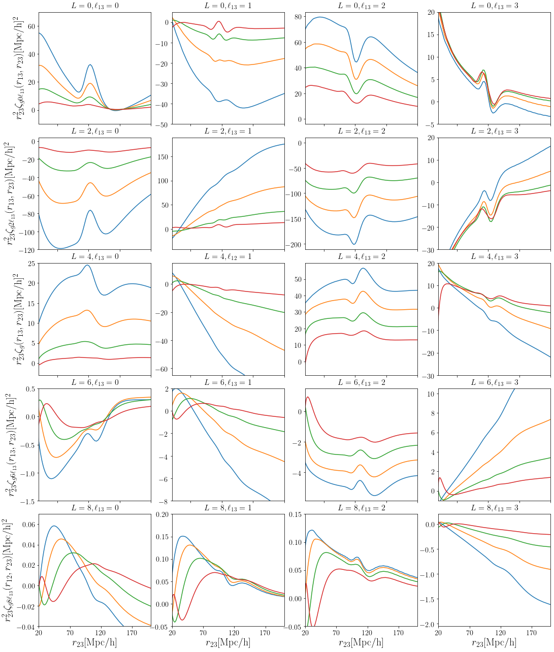
Figure 3: The multipoles of the anisotropic 3PCF for the H$\alpha$ emission line galaxy at $z=1.0$ with first few shape multipoles $\ell_{13}=0-3$. We set $r_{13}=[5,7,10,20]=$ [blue, yellow, green, red]. Only even LoS multipoles are induced in the Newtonian limit while for the shape multipoles both odd and even are induced. The BAO features appear in all the LoS multipoles but it is weaker for shape odd multipoles.

We find that similar to what is obtained in Fourier space in Scoccimarro basis [14], only even LoS multipoles are induced in the Newtonian limit, while for the shape multipoles both odd and even multipoles are induced. The BAO features appear in all the LoS multipoles but it is weaker for the first few shape odd multipoles. In other words, the BAO features are more prominent in the first few shape even multipole moments. The study of the BAO features could focus on those multipoles. One other important feature to note in Figure 3 is that the absolute value of the amplitude of the quadrupole moment ($L=2$) is greater than the amplitude of the monopole moment ($L=0$). This is likely due to the nonlinear bias parameter. The nonlinear bias parameter for the H$\alpha$ emission line galaxy is negative [35], see also equation (2.4). The negative nonlinear bias parameter leads to a reduction in the effective amplitude of the monopole moment relative to the quadrupole moment. This can also be seen analytically in equation (2.12).

2.3 Comparison with previous works

The most recent work on anisotropic 3PCF was given in [17]. The authors decomposed $\zeta_{g}$ in tri-polar spherical harmonics as given in equation (1.3). Here we derive the relationship with the formalism we discussed. We make use of the orthonormality condition for $S_{\ell_{1}\ell_{2}L}$

$$\int{d}^{2}\hat{\bm{r}}_{13}\int{d}^{2}\hat{\bm{r}}_{23}\int{d}^{2}{{\bf\hat{n}}}S_{\ell_{1}\ell_{2}\ell_{3}}(\hat{\bm{r}}_{13},\hat{\bm{r}}_{23},{{\bf\hat{n}}})S_{\ell^{\prime}_{1}\ell^{\prime}_{2}\ell^{\prime}_{3}}(\hat{\bm{r}}_{13},\hat{\bm{r}}_{23},{{\bf\hat{n}}})=\delta_{\ell_{1}\ell^{\prime}_{1}}\delta_{\ell_{2}\ell^{\prime}_{2}}\delta_{\ell_{3}\ell^{\prime}_{3}}\,.$$ (2.33)

The normalisation of the spherical harmonics used in [17] differs from ours. The relationship between $\zeta_{g\ell_{1}\ell_{2}L}$ and $\zeta^{\phi_{n}}_{gL\ell_{2}}$ given in equation (2.31) maybe obtained by using equation (1.3) and (2.33)

$$\zeta_{g\ell_{1}\ell_{2}L}({r}_{13},{r}_{23}) = J_{\ell_{1}\ell_{2}L}\zeta^{\phi_{n}}_{gL\ell_{2}}({r}_{13},{r}_{23})\,,$$ (2.34)

where $J_{\ell_{1}\ell_{2}L}$ is a numerical coefficient

$$J_{\ell_{1}\ell_{2}L}=\sqrt{\frac{(4\pi)^{3}(2\ell_{1}+1)}{(2\ell_{2}+1)(2L+1)}}\begin{pmatrix}\ell_{1}&\ell_{2}&L\\ 0&0&0\end{pmatrix}\,.$$ (2.35)

Comparing this to equation (2.31), we find that $\ell_{2}$ corresponds to $\ell_{12}$ and $\ell_{1}$ corresponds to $\ell_{3}$. The 3j symbol is zero except when $|\ell_{2}-L|\leq\ell_{1}\leq\ell_{2}+L$ which is in agreement with our result. Our coefficient differs because [17] used a different normalisation for the spherical harmonics. The relationship between equation (1.2) introduced in [12, 13] and equation (2.34) was discussed in [17].

3 Covariance of the multipoles of the galaxy 3PCF

We define the estimator of the azimuthal angled ($\phi_{n}$-averaged) multipole moments of the radially binned 3PCF as

$$\hat{\zeta}_{\ell_{13}L}(\bar{r}_{13},\bar{r}_{23}) \equiv \int\frac{d^{3}{\bm{r}}_{13}}{V_{13}}\int\frac{d^{3}{\bm{r}}_{23}}{V_{23}}\int\frac{d\phi_{n}}{2\pi}{\int\frac{d^{2}{{\bf\hat{n}}}}{4\pi}}\,Z_{\ell_{13}L\ell_{3}}(\hat{\bm{r}}_{13},\hat{\bm{r}}_{23},{{\bf\hat{n}}})\zeta_{g}({\bm{r}}_{13},{\bm{r}}_{23},{{\bf\hat{n}}})\,,$$ (3.1)

where $|\ell_{13}-L|\leq\ell_{3}\leq\ell_{13}+L$, the ‘hat’ on thick English alphabets denotes angular component, we decompose the volume integral into radial and angular components

$$\int\frac{d^{3}{\bm{r}}_{13}}{V_{13}}=\frac{1}{V_{13}}\int_{r_{13}-\frac{\Delta r_{13}}{2}}^{r_{!3}+\frac{\Delta r_{13}}{2}}{d}r_{13}r^{2}_{13}\int{{d}}^{2}{\hat{\bm{r}}_{13}}\,,$$ (3.2)

and $V_{13}$ is the effective volume of the radial bin

$$V_{13}=\frac{4\pi}{3}\left(r_{13,\rm{max}}^{3}-r^{3}_{13,\rm{min}}\right)\approx 4\pi r_{13}^{2}\Delta r_{13}\,.$$ (3.3)

We made a thin-bin approximation in the second equality. We introduced the width of the radial bin $\Delta r_{13}$. Also, we absorbed some of the geometric factors in equation (3.1) into $Z_{\ell_{13}L\ell_{3}}$

$$Z_{\ell_{13}L\ell_{3}}(\hat{\bm{r}}_{13},\hat{\bm{r}}_{23},{{\bf\hat{n}}})\equiv\frac{(2L+1)(2\ell_{13}+1)}{\mathcal{H}_{\ell_{13},L,\ell_{3}}}\sum_{m_{13}Mm_{3}}\left({\begin{array}[]{ccc}\ell_{13}&L&\ell_{3}\\ m_{13}&{M}&m_{3}\\ \end{array}}\right)Y^{\ast}_{\ell_{3}m_{3}}(\hat{\bm{r}}_{13})Y^{\ast}_{\ell_{13}m_{13}}(\hat{\bm{r}}_{23})Y_{LM}({{\bf\hat{n}}})\,.$$ (3.6)

Furthermore, we define the anisotropic 3PCF with galaxies at the vertices of the triangle as

$$\zeta_{g}({\bm{r}}_{13},{\bm{r}}_{23},{{\bf\hat{n}}})\equiv\frac{1}{V_{s}}\int{d}^{3}r_{3}\Delta_{g}({\bm{r}}_{3}+{\bm{r}}_{13})\Delta_{g}({\bm{r}}_{3}+{\bm{r}}_{23})\Delta_{g}({\bm{r}}_{3})\,,$$ (3.7)

where $V_{s}$ is the volume of the survey. This allows to average over translations allowing every point in the survey to serve as ${\bm{r}}_{3}$. There is a clever way of estimating equation (3.7) from a given survey or catalogue in $\mathcal{O}(N^{2})$ time described in [8], further development in this direction was recently reported in [46]. From equation (3.1), we define the covariance matrix of the multipole moments of the azimuthal angle averaged 3PCF as

$${{\rm{Cov}}\left[\hat{\zeta}_{\ell_{13}L}(r_{13},r_{23}),\hat{\zeta}_{\ell^{\prime}_{13}L^{\prime}}(r^{\prime}_{13},r^{\prime}_{23})\right]} = \int\frac{{{d}}^{2}{r}_{13}}{V_{13}}\int\frac{{{d}}^{2}{r}_{23}}{V_{23}}\int\frac{{d}^{2}{r}^{\prime}_{13}}{V_{13}}\int\frac{{d}^{2}{r}^{\prime}_{23}}{V_{23}}\int\frac{d\phi_{n}}{2\pi}\int\frac{d\phi^{\prime}_{n}}{2\pi}\int{\frac{{d}^{2}{{\bf\hat{n}}}}{4\pi}}\,\,\,\,$$

$$\times\int{\frac{{d}^{2}{{\bf\hat{n}}}^{\prime}}{4\pi}}Z_{\ell_{13}\ell_{3}L}Z_{\ell^{\prime}_{13}\ell^{\prime}_{3}L^{\prime}}{\rm{Cov}}\left[\zeta_{g}({\bm{r}}_{13},{\bm{r}}_{23},{{\bf\hat{n}}})\zeta_{g}({\bm{r}}^{\prime}_{13},{\bm{r}}^{\prime}_{23},{{\bf\hat{n}}}^{\prime})\right]\,,$$

In the plane-parallel limit, it is easier to calculate ${\rm{Cov}}\left[\zeta_{g}({\bm{r}}_{13},{\bm{r}}_{23},{{\bf\hat{n}}})\zeta_{g}({\bm{r}}^{\prime}_{13},{\bm{r}}^{\prime}_{23},{{\bf\hat{n}}}^{\prime})\right]$ in Fourier space

$${\rm{Cov}}\left[\zeta_{g}({\bm{r}}_{13},{\bm{r}}_{23},{{\bf\hat{n}}})\zeta_{g}({\bm{r}}^{\prime}_{13},{\bm{r}}^{\prime}_{23},{{\bf\hat{n}}}^{\prime})\right] = \int\frac{{d}^{3}k_{1}}{(2\pi)^{3}}\int\frac{{d}^{3}k_{2}}{(2\pi)^{3}}\int\frac{{d}^{3}k^{\prime}_{1}}{(2\pi)^{3}}\int\frac{{d}^{3}k^{\prime}_{2}}{(2\pi)^{3}}e^{i{\bm{k}}_{1}\cdot{\bm{r}}_{13}+i{\bm{k}}_{2}\cdot{\bm{r}}_{23}}$$

$$\times e^{i{\bm{k}}^{\prime}_{1}\cdot{\bm{r}}^{\prime}_{13}+i{\bm{k}}^{\prime}_{2}\cdot{\bm{r}}^{\prime}_{23}}{\rm{Cov}}\left[B_{g}({\bm{k}}_{1},{\bm{k}}_{2},-{\bm{k}}_{12})B_{g}({\bm{k}}^{\prime}_{1},{\bm{k}}^{\prime}_{2},-{\bm{k}}^{\prime}_{12})\right]\,,$$

where ${\bm{k}}_{12}={\bm{k}}_{1}+{\bm{k}}_{2}$ and we have made use of the Fourier transformation of $\zeta_{g}$ given in equation (2.9). We take the Gaussian limit of the galaxy bispectrum covariance given in [47]

$${\rm{Cov}}\left[{B}_{g}({\bm{k}}_{1},{\bm{k}}_{2},-{\bm{k}}_{12}){B}_{g}({\bm{k}}^{\prime}_{1},{\bm{k}}^{\prime}_{2},-{\bm{k}}^{\prime}_{12})\right] = {{\frac{(2\pi)^{6}}{V_{s}}}}\bigg{[}\delta^{D}({\bm{k}}_{1}+{\bm{k}}_{1}^{\prime})\delta^{D}({\bm{k}}_{2}+{\bm{k}}_{2}^{\prime})+\delta^{D}({\bm{k}}_{2}+{\bm{k}}_{1}^{\prime})\delta^{D}({\bm{k}}_{1}+{\bm{k}}_{2}^{\prime})$$ (3.10)

$$+4{\rm{perms.}}\bigg{]}\left(\hat{P}_{g}({\bm{k}}_{1})\hat{P}_{g}({\bm{k}}_{2})\hat{P}_{g}({\bm{k}}_{12})\right)\,,$$

where $\hat{P}_{g}$ is decomposed into the theory power spectrum and the shot noise: $\hat{P}_{g}({\bm{k}})=P_{g}({\bm{k}})+{1/{n_{g}}},$ $P_{g}$ is the theory galaxy power spectrum and $n_{g}$ is the galaxy number density. Since we average over all possible positions of the galaxy at ${\bm{r}}_{3}$ vertex, we focus only on the configuration that contribute to the covariance matrix with translation about the $[{\bm{r}}_{3},{\bm{r}}^{\prime}_{3}]$ vertex

$${\rm{Cov}}\left[\zeta_{g}({\bm{r}}_{13},{\bm{r}}_{23},{{\bf\hat{n}}})\zeta_{g}({\bm{r}}^{\prime}_{13},{\bm{r}}^{\prime}_{23},{{\bf\hat{n}}}^{\prime})\right] = \frac{1}{V_{s}}\int\frac{{d}^{3}k_{1}}{(2\pi)^{3}}\int\frac{{d}^{3}k_{2}}{(2\pi)^{3}}\bigg{[}e^{ik_{1}\left[{\bm{r}}_{13}-{\bm{r}}^{\prime}_{13}\right]}e^{ik_{2}\left[{\bm{r}}_{23}-{\bm{r}}^{\prime}_{23}\right]}$$

$$+e^{ik_{1}\left[{\bm{r}}_{13}-{\bm{r}}^{\prime}_{23}\right]}e^{ik_{2}\left[{\bm{r}}_{23}-{\bm{r}}^{\prime}_{13}\right]}\bigg{]}\left(\hat{P}_{g}({\bm{k}}_{1})\hat{P}_{g}({\bm{k}}_{2})\hat{P}_{g}({\bm{k}}_{12})\right)\,.$$

Expanding the exponentials in plane wave and working through a very lengthy algebra (see appendix D) gives

$${{\rm{Cov}}\left[\hat{\zeta}_{\ell_{13}L}(r_{13},r_{23}),\hat{\zeta}_{\ell^{\prime}_{13}L^{\prime}}(r^{\prime}_{13},r^{\prime}_{23})\right]} = \sum_{L\ell_{12}}\mathcal{O}_{LL^{\prime}L_{2}}^{\ell_{13}\ell^{\prime}_{13}\ell_{12}}\int\frac{{d}k_{1}}{k_{1}}\int\frac{{d}k_{2}}{k_{2}}\Delta^{PPP}_{L_{2}\ell_{12}}({k_{1},k_{2}})$$

$$\times\mathcal{J}_{\ell_{3}\ell^{\prime}_{3}}^{\ell_{13}\ell^{\prime}_{13}}(k_{1},k_{2},\bar{r}_{13},\bar{r}_{23},\bar{r}^{\prime}_{13},\bar{r}^{\prime}_{23})\,,\qquad\quad$$

where we have introduced the multipole moment of the product of three power spectra

$$\Delta^{PPP}_{L_{2}\ell_{12}}({k_{1},k_{2}}) \equiv \frac{k_{1}^{3}k_{2}^{3}\left(\hat{P}({k}_{1})\hat{P}({k}_{2})\hat{P}({k}_{12})\right)^{\phi_{n}}_{L_{2}\ell_{12}}}{V_{s}(2\pi^{2})^{2}}\,.$$ (3.13)

The multipole moments of the product of the three power spectra are obtained using

$$\left(P({k}_{1})P({k}_{2})P({k}_{12})\right)^{\phi_{n}}_{L\ell_{12}} = {{(2\ell_{12}+1)\over 2}}{{(2L+1)\over 2}}\int_{-1}^{1}{d}\mu_{1}\int_{-1}^{1}{d}\mu_{12}\int_{0}^{2\pi}\frac{{{d}}\phi_{n}}{2\pi}$$

$$\qquad\times~{}\left(P_{g}({k}_{1},\mu_{1})P_{g}({k}_{2},\mu_{2})P_{g}({k}_{12},\mu_{3})\right)\mathcal{L}_{L}(\mu_{1})\mathcal{L}_{\ell_{12}}(\mu_{12})\,.$$

In the plane-parallel limit for a closed triangle, the three angles are related as shown in equation (C.18). In equation (3), we introduced

$$\mathcal{O}_{LL^{\prime}L_{2}}^{\ell_{13}\ell^{\prime}_{13}\ell_{12}.} \equiv (i)^{\ell_{3}+\ell_{13}}(-i)^{\ell_{3}^{\prime}+\ell_{13}^{\prime}}\frac{(2L+1)(2\ell_{13}+1)(2L^{\prime}+1)(2\ell^{\prime}_{13}+1)}{(4\pi)^{2}(2L_{2}+1)(2\ell_{12}+1)}$$

$$\times\sum_{L_{3}=|\ell^{\prime}_{3}-\ell_{3}^{\prime}|}^{\ell^{\prime}_{3}+\ell_{3}^{\prime}}\frac{\mathcal{H}_{\ell_{3}\ell^{\prime}_{3}L_{3}}^{0,0,0}\mathcal{H}_{\ell_{12}L_{2}L_{3}}^{0,0,0}\mathcal{H}_{\ell_{13}\ell^{\prime}_{13}\ell_{12}}^{0,0,0}\mathcal{H}_{LL^{\prime}L_{2}}^{0,0,0}}{{\mathcal{H}^{0,0,0}_{\ell_{13},L,\ell_{3}}\mathcal{H}^{0,0,0}_{\ell^{\prime}_{13},L^{\prime},\ell^{\prime}_{3}}}}\begin{Bmatrix}\ell_{13}&L&\ell_{3}\\ \ell^{\prime}_{13}&L^{\prime}&\ell^{\prime}_{3}\\ \ell_{12}&L_{2}&L_{3}\end{Bmatrix}\,,$$

where the big Curly bracket is the $9j$ symbol [18] and $\mathcal{H}_{\ell_{3}\ell^{\prime}_{3}L_{3}}^{0,0,0}$ is non-zero only when $|L-\ell_{13}|\leq\ell_{3}\leq L+\ell_{13}$ and $|\ell^{\prime}_{13}-L^{\prime}|\leq\ell^{\prime}_{3}\leq\ell^{\prime}_{13}+L^{\prime}$ is satisfied. We brought together all the spherical Bessel functions under one umbrella in the thin-shell limit $\Delta r\ll r$:

$$\mathcal{J}_{\ell_{3}\ell^{\prime}_{3}\ell_{13}\ell^{\prime}_{13}}(k_{1},k_{2},\bar{r}_{13},\bar{r}_{23},\bar{r}^{\prime}_{13},\bar{r}^{\prime}_{23}) = \bigg{[}j_{\ell_{3}}(k_{1}\bar{r}_{13})j_{\ell_{3}^{\prime}}(k_{1}\bar{r}^{\prime}_{13})j_{\ell_{13}}(k_{2}\bar{r}_{23})j_{\ell_{13}^{\prime}}(k_{2}\bar{r}^{\prime}_{23})$$

$$+j_{\ell_{3}}(k_{1}\bar{r}_{13})j_{\ell_{3}^{\prime}}(k_{1}\bar{r}^{\prime}_{23})j_{\ell_{13}}(k_{2}\bar{r}_{23})j_{\ell_{13}^{\prime}}(k_{2}\bar{r}^{\prime}_{13})\bigg{]}\,.$$

We show in appendix B how to calculate the covariance of the anisotropic 3PCF multipole moments (equation (3)) using FFTLog formalism. This formalism allows to decompose $\Delta^{PPP}_{L_{2}\ell_{12}}({k_{1},k_{2}})$ into a finite number of power-laws (see equation (B.2)) which then makes it easier to perform the integration over the spherical Bessel functions analytically

$$\int\frac{{d}k_{1}}{k_{1}}{k_{1}^{\beta_{1}+i\eta_{m}}}j_{\ell_{3}}(k_{1}\bar{r}_{13})j_{\ell_{3}^{\prime}}(k_{1}\bar{r}^{\prime}_{13})=\frac{r_{13}^{-i\eta_{m}}}{r_{13}^{\beta_{1}}}\,\int_{0}^{\infty}{d}x_{1}\,x_{1}^{{\beta_{1}+i\eta_{m}}-1}j_{\ell_{3}}(x_{1})j_{\ell^{\prime}_{3}}(x_{1}y_{1})\,,$$ (3.17)

where $x_{1}=k_{1}\bar{r}_{13}$ and $y_{1}=\bar{r}^{\prime}_{13}/\bar{r}_{13}$. The integral on the RHS has an analytical solution in terms of the hypergeometric function ${}_{2}F_{1}$ [18, 48], (see equation (B.9) for details)

$${I}_{\ell_{3}\ell^{\prime}_{3}}(\omega_{m},y_{n}) \equiv 4\pi\int_{0}^{\infty}{d}x\,x^{\omega_{m}-1}j_{\ell_{3}}(x)j_{\ell^{\prime}_{3}}(xy_{n})\delta_{\ell_{3}\ell^{\prime}_{3}}$$ (3.18)

$$= \frac{2^{\omega_{m}-1}\pi^{2}\Gamma(\ell_{3}+\frac{\omega_{m}}{2})}{\Gamma(\frac{3-\omega_{m}}{2})\Gamma(\ell_{3}+\frac{3}{2})}\,y_{n}^{\ell_{3}}\,{}_{2}F_{1}\Bigg{[}\begin{array}[]{c}\frac{\omega_{m}-1}{2},\ell_{3}+\frac{\omega_{m}}{2},\ell_{3}+\frac{3}{2}\end{array}\Bigg{|}\,y_{n}^{2}\Bigg{]}\quad(|y_{n}|\leq 1)\,,$$ (3.20)

where $\Gamma$ is the gamma function and we focus on the limit where $\ell_{3}=\ell^{\prime}_{3}$. For $|y_{n}|\geq 1$, we use the following property ${I}_{\ell\ell^{\prime}}(\omega_{m},y_{n})=y_{n}^{\ell}{I}_{\ell\ell^{\prime}}(\omega_{m},1/y_{n})$ [49].

3.1 Estimate of the signal to noise ratio

Using the 2D FFTLog formalism (see Appendix B for all the technical details on how this is done), we compute the signal to noise ratio (SNR) for the monopole, quadrupole and hexadecapole of the anisotropic 3PCF for a typical galaxy redshift survey with volume and number density given in Figure 7 and the tracer bias parameters are given in equations (2.3) and (2.4).

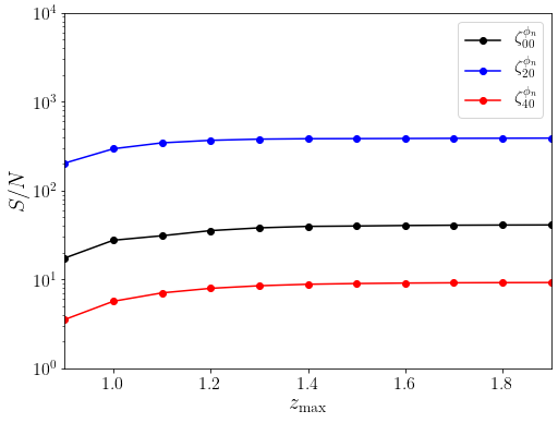
Figure 4: This is the signal to noise ratio for the first three multipole moments of the anisotropic 3PCF, i.e. $L=0,2,4$ with $\ell_{13}=0$. $\ell_{13}$ corresponds to the monopole limit of the triangular shape. We set the radial bin width to $\Delta r_{13}=\Delta r_{23}=0.5[{\rm{Mpc}}/h]$ and the range of the radial scales to $[r_{\rm{min}},r_{\rm{max}}]=[40,120][{\rm{Mpc}}/h]$. The SNR of the LoS quadrupole moment is much greater than the LoS monopole.

The survey covers the redshift range of $0.9$ to $2.0$ and we split it into 10 redshift bins with the width of $0.1$. We estimate the SNR in the Gaussian limit(see equations (B.15) to (B.18) on how Gaussian limit is obtained) using

$$\left(\frac{S}{N}\right)^{2} = \sum_{z_{\rm{min}}}^{z_{\rm{max}}}\sum_{r_{13}r_{23}}\frac{{{\zeta}^{\phi_{n}}_{L\ell_{13}}(\bar{r}_{13},\bar{r}_{23})}{{\zeta}^{\phi_{n}}_{L\ell_{13}}(\bar{r}_{13},\bar{r}_{23})}}{{\rm{Var}}\left[\hat{\zeta}_{\ell_{13}L}(\bar{r}_{13},\bar{r}_{23})\hat{\zeta}_{\ell_{13}L}(\bar{r}_{13},\bar{r}_{23})\right]}\,.$$ (3.21)

We neglect the Alcock-Paczynski effects and the loop corrections for simplicity [50]. The cosmological parameters are fixed to the Planck values [29] during the computation, the tracer bias parameters evolve according to equations (2.3) and (2.4). Without loss of generality, we set $\ell_{13}=0$ and focus on the first three even multipole (i.e $L\in$ even). In the rest of the analysis, we set the radial bin width to $\Delta r_{13}=\Delta r_{23}=0.5$ [Mpc/h]. The result is shown in Figure 4. Unfortunately, the tree-level approximation of the 3PCF we have used is not expected to be valid on small scales. Therefore, we set $[r_{13\rm{min}},r_{23\rm{min}}]=[40,40]$ [Mpc/h] and $[r_{13\rm{max}},r_{23\rm{max}}]=[120,120][{\rm{Mpc}}/h]$. Note that the SNR for the LoS quadrupole moment is greater than the LoS monopole moment. This can easily be understood by looking at the amplitude of the quadrupole moment shown in Figure 3. The absolute value of the quadrupole moment of the anisotropic 3PCF is greater than the monopole moment, this difference get propagated to the SNR as well.

4 Conclusion

We have shown how the computational difficulties associated with the estimation and high-dimensionality of the anisotropic 3PCF may be alleviated by using the 2D FFTLog formalism and the concept of decomposing all its angular dependence in multipole moments respectively. We showed that this can be done in the so-called Scoccimarro basis which was first introduced in [15] to reduce the dependence of the anisotropic galaxy bispectrum in Fourier space from nine to five free parameters: three parameters characterise the triangle’s shape, e.g. two sides and the enclosed angle, and the remaining two describe the orientation of the triangle with respect to the line of sight. We showed how to consistently map the anisotropic galaxy bispectrum in this basis to the corresponding basis in configuration space for the anisotropic 3PCF, then we focused exclusively on the limit where the azimuthal degree of freedom is averaged over leading to the azimuthal angle-averaged 3PCF. Our result is an extension of the formalism introduced in [9] in real space. It was extended to only the monopole moment (isotropic limit) in [11]. Furthermore, we derived for the first time the full expression for the covariance matrix of the azimuthal angled averaged auto 3PCF in plane parallel limit.

This approach involves expanding all angular dependence i.e. information associated with triangle shapes and the information associated with orientation of the triangle respect to the LoS direction in two different Legendre polynomials respectively. This allows for a quick assessment of the total information content of the 3PCF by studying only the first few multipoles moments. It significantly reduces the need to invest huge resources in evaluating complicated combinatorial problem associated with different triangle configurations [9]. With the extension to anisotropic 3PCF that we have shown here, we are hopeful that this contribution will help to elevate the use of the 3PCF as a reliable tool for cosmological inference just as the anisotropic 2PCF especially for probing the imprint of the primordial non-Gaussainity on the large scale structure.

Finally, the multipole moments of the galaxy 3PCF we derived contain two momentum integrals of the product of the galaxy bispectrum and the two spherical Bessel functions. The presence of a double momentum integrals over a highly oscillating spherical Bessel functions makes it intractable to calculate using the traditional numerical integration algorithm such as Quadrature or related methods. We have shown how this difficulty maybe circumvented by using the 2D FFTLog formalism, which allows to decompose the dimensionless galaxy bispectrum in a finite number of power-laws and then perform the integrals over the oscillating spherical Bessel functions analytically. The 2D FFTLog formalism we use was developed in [19]. It allows to optimally perform these integrals in $\mathcal{O}\left(N\log N\right)$ times, where $N$ is the number of 2D-grid points . We show that each multipole moment of the anisotropic 3PCF has a discernible BAO features at the expected scale $100[\rm{Mpc}/h]$. In comparison to the 2PCF, we find that at each multipole, the amplitude of the multipole moment of the 3PCF and its corresponding BAO bump depends sensitively on the shape of the triangle. In the limit where one side of the triangle is fixed at small scale, we found a more pronounced BAO peak as we move the fixed side of the triangle deeper into small scales.

Appendix A Double integration of the 3PCF using 2D FFTLOG

One of the key results of the paper is the full expression for the $\phi_{n}$-averaged anisotropic 3PCF

$$\zeta_{gL\ell_{12}}({r}_{12},{r}_{23}) = i^{2\ell_{12}+L}\int_{0}^{\infty}\frac{{d}k_{1}}{k_{1}}\int_{0}^{\infty}\frac{{d}k_{2}}{k_{2}}\Delta^{{\rm{RSD}}}_{{\rm{B}}L\ell_{12}}(k_{1},k_{2})j_{\ell_{12}+L}(k_{1}r_{12})j_{\ell_{12}}(k_{2}r_{23})\,,$$ (A.1)

where have $\Delta^{{\rm{RSD}}}_{{\rm{B}}L\ell_{12}}$ is the dimensionless galaxy bispectrum, $L$ is an integer which indicates the multipole moment with respect to the line of sight, $\ell_{12}$ is an integer which indicates the multipole moment associated with the angle between any two sides of the triangle formed by the galaxy triplet.

An attempt to perform the integrations in equation (2.32) or (1.1) using any of the Quadrature methods leads to a sub-optimal result for cosmological inference. This has obvsiouly limited its use despite the amount of cosmological information it contains. On a close examination, the two biggest stumbling blocks in performing integration in equation (1.1) or (2.32) is the presence of the two spherical Bessel functions in the double integral and the fact that $\Delta^{{\rm{RSD}}}_{{\rm{B}}L\ell_{12}}$ is not in separable in general. Recently, [19] proposed a cosmolgically optimal technique to perform the kind of double integrals in equation (2.32). This technique is based on FFTLOG proposal for 1D integrals proposed in [51, 52] and applied to the two-point correlation function in [20]. The methods involves decomposing the dimensionless bispectrum $\Delta^{{\rm{RSD}}}_{{\rm{B}}L\ell_{12}}(k_{1},k_{2})$ into a series of products of two power-laws in the $\log k_{1}$-$\log k_{2}$ space [53, 54, 55, 19]

$${\Delta^{{\rm{RSD}}}_{{\rm{B}}L\ell_{12}}(k_{p},k_{q})}=\sum_{m=-N_{p}/2}^{N_{p}/2}\sum_{n=-N_{q}/2}^{N_{q}/2}{c}_{L\ell_{12}mn}\left(\frac{k_{1}^{\beta_{1}+i\eta_{m}}}{k_{10}^{i\eta_{m}}}\right)\left(\frac{k_{2}^{\beta_{2}+i\eta_{n}}}{k_{20}^{i\eta_{n}}}\right)\,,$$ (A.2)

where ${c}_{mn}$ is the filtered Fourier coefficients of the dimensional galaxy bispectrum

$${c}_{L\ell_{12}mn}=\frac{W_{m}W_{n}}{N_{p}N_{q}}\sum_{p=0}^{N_{p}-1}\sum_{q=0}^{N_{q}-1}\frac{\Delta^{{\rm{RSD}}}_{{\rm{B}}L\ell_{12}}(k_{p},k_{q})}{k_{p}^{\beta_{1}}k_{q}^{\beta_{2}}}\exp^{-{2\pi i}\left(\frac{m_{p}}{N_{p}}+\frac{n_{q}}{N_{q}}\right)}~{},$$ (A.3)

where $W_{m},W_{n}$ are the $m$-th and $n$-th elements of the 1D window function $\mathbf{W}$ introduced to avoid ringing at the edges [53], $N_{x}$ is the size of the $k_{x}$ array, $\beta_{1},\beta_{2}$ are the real parts of the power law indices for $k_{p}$ and $k_{q}$ arrays. The frequencies are defined with respect to linear space in $\ln k$

$$\eta_{m}=2\pi\frac{m}{(N\Delta_{\ln k})}=2\pi\frac{m}{\log(k_{\rm{max}}/k_{\rm{min}})}\,,\qquad{\rm{with}}\quad\Delta_{\ln k}=\frac{1}{N}\log\left(\frac{k_{\rm{max}}}{k_{\rm{min}}}\right)$$

$\Delta_{\ln k}$ is the linear spacing in $\ln k$. For example, given a $k_{q}$ array, each Fourier mode are separated according to $k_{q}=k_{q0}\exp(q\Delta_{\ln k})$ with $k_{q0}$ being the smallest value in the $k_{q}$ array. The most time consuming part of this calculation is the discretization of $\Delta^{{\rm{RSD}}}_{{\rm{B}}L\ell_{12}}(k_{1},k_{2})$ into an $N_{p}\times N_{q}$ grid. There are many options available to help speed up the computation, for example using a highly optimsed numpy array in python [56] or using xtensor-stack in c++ with OpenMP support (https://xtensor.readthedocs.io/en/latest/). Using equation (A.2) in equation (A.1) gives

$$\zeta_{gL\ell_{12}}({r}_{12},{r}_{23}) = {i^{\ell_{12}+\ell_{3}}}\sum_{m=-N_{p}/2}^{N_{p}/2}\sum_{n=-N_{q}/2}^{N_{q}/2}\frac{{c}_{L\ell_{12}mn}}{k_{10}^{i\eta_{m}}k_{20}^{i\eta_{n}}}$$

$$\times\int_{0}^{\infty}\frac{dk_{1}}{k_{1}}k_{1}^{\beta_{1}+i\eta_{m}}j_{\ell_{12}}(k_{1}r_{13})\int_{0}^{\infty}\frac{dk_{2}}{k_{2}}k_{2}^{\beta_{2}+i\eta_{n}}j_{\ell_{3}}(k_{2}r_{23})\,.$$

The $k$-integrals may be performed after a change of variables $x_{1}=k_{1}r_{13}$ and $x_{2}=k_{2}r_{23}$, for example

$$\int_{0}^{\infty}\frac{dk_{1}}{k_{1}}k_{1}^{\beta_{1}+i\eta_{m}}j_{\ell_{12}}(k_{1}r_{13})=\frac{r_{13}^{-i\eta_{m}}}{r_{13}^{\beta_{1}}}\,\int_{0}^{\infty}{{d}x}\,x^{{\beta_{1}+i\eta_{m}}-1}j_{\ell}(x)\,.$$ (A.5)

The integral in this form has an analytical solution in terms of the $\Gamma$ functions [57]

$$g_{\ell}(\omega_{n})=\frac{4}{\sqrt{\pi}}\int_{0}^{\infty}{{d}x}\,x^{\omega_{n}-1}j_{\ell}(x)=2^{\omega_{n}}\frac{\Gamma\left(\frac{\ell+\omega_{n}}{2}\right)}{\Gamma\left(\frac{3+\ell-\omega_{n}}{2}\right)}\,.$$ (A.6)

For $\omega_{m}=\beta_{1}+i\eta_{m}$ and the range of validity of the bias parameters are $-\ell_{1}<\beta_{1}<2$ and $-\ell_{2}<\beta_{2}<2$. In order to avoid singularities in $\Gamma$, non-integer values for $\beta_{1},\beta_{2}$ are usually chosen. We set $\beta_{1}=\beta_{2}=1.01$ throughout our computation. Putting equation (A.6) in equation (A) gives

$$\zeta_{gL\ell_{13}}({r}_{13},{r}_{23}) = \frac{\pi i^{2\ell_{13}+L}}{16r_{13}^{\beta_{1}}r_{23}^{\beta_{2}}}\sum_{m=-N_{p}/2}^{N_{p}/2}\sum_{n=-N_{q}/2}^{N_{q}/2}{{c}_{L\ell_{13}mn}}{(k_{p0}r_{13})^{-i\eta_{m}}(k_{q0}r_{23})^{-i\eta_{n}}}$$

$$\times g_{\ell_{13}}(\beta_{1}+i\eta_{m})g_{\ell_{12}+L}(\beta_{2}+i\eta_{n})~{}\,.$$

Following [19] we take full advantage of the FFTLog algorithm, we assume that $r_{13},r_{23}$ are identical arrays and logarithmically sampled with a corresponding linear spacing, for example $\Delta_{\ln r_{13}}$ in $\ln r_{13}$, with $\Delta_{\ln r_{13}}=\Delta_{\ln k_{1}}$ and $\Delta_{\ln r_{23}}$ in $\ln r_{23}$, with $\Delta_{\ln r_{23}}=\Delta_{\ln k_{2}}$, i.e $r_{13q}=r_{130}\exp(q\Delta_{\ln r})$ with $r_{130}$ being the smallest value in the $r_{13q}$ array. Since the values of $r_{13}$ and $,r_{23}$ are independent of the $\{k_{p},k_{q}\}$ arrays, the summation in equation (A) can be written as

$$\zeta_{gL\ell_{13}}({r}_{13},{r}_{23}) = \frac{\pi i^{2\ell_{12}+L}}{16r_{p12}^{\beta_{1}}r_{q23}^{\beta_{2}}}{\rm{IFFT2}}\bigg{[}{{c}^{\ast}_{L\ell_{13}mn}}{(k_{p0}r_{120})^{i\eta_{m}}(k_{q0}r_{230})^{i\eta_{n}}}$$

$$\times g_{\ell_{12}}(\beta_{1}-i\eta_{m})g_{\ell_{12}+L}(\beta_{2}-i\eta_{n})\bigg{]}\,.$$

Here $r_{13p},r_{23q}$ ($p,q=0,1,\cdots,N-1$) are the $p$-th and $q$-th elements in the $r_{13}$ and $r_{23}$ array, respectively. We made use of $e^{2\pi im}$. IFFT2 stands for the two-dimensional Inverse Fast Fourier Transform. We use a modified version of the open source code by [19] to calculate equation (A).

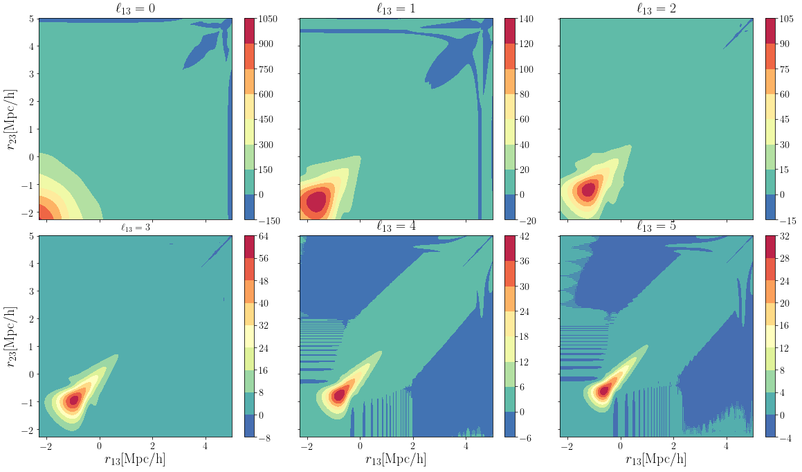
Figure 5: The 2D heat map in log-scale of the real space 3PCF at different (shape) multipole moment. Here we show the first six multipoles. The features are symmetric about the diagonal in all the multipoles. This indicates that the 1D plot in Figure 1 captures all the essential features.

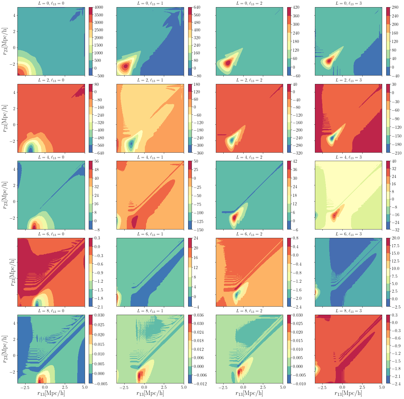
Figure 6: The 2D heat map in log-scale of the multipoles of the anisoptropic 3PCF. In the vertical direction, we have the LOS multipoles starting from $L=0$ (top panel) to $L=8$ (bottom panel), while the horizontal direction, we have the first four multipoles of the triangle configuration. On the first left panel we have $\ell_{13}=0$ and last right panel we have $\ell_{13}=3$. The heat map indicates the amplitude of the 3PCF. Note that the symmetry about the major diagonal seen in the multipole of the real space 3PCF starts to disappear for the anisotropic 3PCF especially at higher LOS multipole moments.

Appendix B Double integration of the covariance matrix using 2D FFTLOG

We shall now describe how we calculate the covariance of the multipoles of the 3PCF using 2D FFTLOG formalism. We start from equation (3)

$${\rm{Cov}}\left[\hat{\zeta}_{\ell_{13}L}(r_{13},r_{23})\hat{\zeta}_{\ell^{\prime}_{13}L^{\prime}}(r^{\prime}_{13},r^{\prime}_{23})\right] = \sum_{L\ell_{12}}\mathcal{O}_{LL^{\prime}L_{2}}^{\ell_{13}\ell^{\prime}_{13}\ell_{12}.}\int\frac{{d}k_{1}}{k_{1}}\int\frac{{d}k_{2}}{k_{2}}\Delta^{PPP}_{L_{2}\ell_{12}}({k_{1},k_{2}})$$ (B.1)

$$\times\mathcal{J}_{\ell_{3}\ell^{\prime}_{3}}^{\ell_{13}\ell^{\prime}_{13}}(k_{1},k_{2},\bar{r}_{13},\bar{r}_{23},\bar{r}^{\prime}_{13},\bar{r}^{\prime}_{23})\,,$$

where $\mathcal{J}_{\ell_{3}\ell^{\prime}_{3}}^{\ell_{13}\ell^{\prime}_{13}}$ is defined in equation (3) as a collection of the spherical Bessel functions. The interest is to evaluate the double k-integrals analytically. To be able to do this, we perform a power-law decomposition of $\Delta^{PPP}_{L_{2}\ell_{12}}$

$$\Delta^{PPP}_{L_{2}\ell_{12}}(k_{p},k_{q})=\sum_{m=-N_{p}/2}^{N_{p}/2}\sum_{n=-N_{q}/2}^{N_{q}/2}{c}^{PPP}_{L_{2}\ell_{12}mn}\left(\frac{k_{1}^{\beta_{1}+i\eta_{m}}}{k_{10}^{i\eta_{m}}}\right)\left(\frac{k_{2}^{\beta_{2}+i\eta_{n}}}{k_{20}^{i\eta_{n}}}\right)\,,$$ (B.2)

where ${c}^{PPP}_{mn}$ is the filtered Fourier coefficients of the product of three power spectra

$${c}^{PPP}_{L_{2}\ell_{12}mn}=\frac{W_{m}W_{n}}{N_{p}N_{q}}\sum_{p=0}^{N_{p}-1}\sum_{q=0}^{N_{q}-1}\frac{\Delta^{PPP}_{L_{2}\ell_{12}}(k_{p},k_{q})}{k_{p}^{\beta_{1}}k_{q}^{\beta_{2}}}\exp^{-{2\pi i}\left(\frac{m_{p}}{N_{p}}+\frac{n_{q}}{N_{q}}\right)}\,,$$ (B.3)

where $W_{m}$ is a window function, its proper form is given in [53]. Substituting in equation (B.1) leads to

$${\rm{Cov}}\left[\hat{\zeta}_{\ell_{13}L}\hat{\zeta}_{\ell^{\prime}_{13}L^{\prime}}\right] = \sum_{L_{2}\ell_{12}}\mathcal{O}_{LL^{\prime}L_{2}}^{\ell_{13}\ell^{\prime}_{13}\ell_{12}.}\sum_{m=-N_{p}/2}^{N_{p}/2}\sum_{n=-N_{q}/2}^{N_{q}/2}{c}^{PPP}_{L_{2}\ell_{12}mn}k_{10}^{-i\eta_{m}}{k_{20}^{-i\eta_{n}}}$$

$$\times\bigg{[}\int\frac{{d}k_{1}}{k_{1}}{k_{1}^{\beta_{1}+i\eta_{m}}}j_{\ell_{3}}(k_{1}\bar{r}_{13})j_{\ell_{3}^{\prime}}(k_{1}\bar{r}^{\prime}_{13})\int\frac{{d}k_{2}}{k_{2}}{k_{2}^{\beta_{2}+i\eta_{n}}}j_{\ell_{13}}(k_{2}\bar{r}_{23})j_{\ell_{13}^{\prime}}(k_{2}\bar{r}^{\prime}_{23})$$

$$+\int\frac{{d}k_{1}}{k_{1}}{k_{1}^{\beta_{1}+i\eta_{m}}}j_{\ell_{3}}(k_{1}\bar{r}_{13})j_{\ell_{3}^{\prime}}(k_{1}\bar{r}^{\prime}_{23})\int\frac{{d}k_{2}}{k_{2}}{k_{2}^{\beta_{2}+i\eta_{n}}}j_{\ell_{13}}(k_{2}\bar{r}_{23})j_{\ell_{13}^{\prime}}(k_{2}\bar{r}^{\prime}_{13})\bigg{]}\,.$$

The $k$-integrals over the spherical Bessel functions in equation (B) may be calculated analytically after a change of variables; for example $x_{1}=k_{1}\bar{r}_{13}$,

$$\int\frac{{d}k_{1}}{k_{1}}{k_{1}^{\beta_{1}+i\eta_{m}}}j_{\ell_{3}}(k_{1}\bar{r}_{13})j_{\ell_{3}^{\prime}}(k_{1}\bar{r}^{\prime}_{13})=\frac{r_{13}^{-i\eta_{m}}}{r_{13}^{\beta_{1}}}\,\int_{0}^{\infty}{d}x_{!}\,x_{1}^{{\beta_{1}+i\eta_{m}}-1}j_{\ell_{3}}(x_{1})j_{\ell^{\prime}_{3}}(x_{1}y_{n})\,,$$ (B.5)

where $y_{1}=\bar{r}^{\prime}_{13}/\bar{r}_{13}$. Note that there is a freedom to perform the integration via the following change of variable: $x^{\prime}_{1}=k_{1}\bar{r}^{\prime}_{13}$

$$\int\frac{{d}k_{1}}{k_{1}}{k_{1}^{\beta_{1}+i\eta_{m}}}j_{\ell_{3}}(k_{1}\bar{r}_{13})j_{\ell_{3}^{\prime}}(k_{1}\bar{r}^{\prime}_{13})=\frac{{r^{\prime}}_{13}^{-i\eta_{m}}}{{r^{\prime}}_{13}^{\beta_{1}}}\,\int_{0}^{\infty}{d}x^{\prime}_{!}\,{x^{\prime}}_{1}^{{\beta_{1}+i\eta_{m}}-1}j_{\ell^{\prime}_{3}}(x^{\prime}_{1})j_{\ell_{3}}(x^{\prime}_{1}/y_{n})\,.$$ (B.6)

This freedom could be understood as a consequence of the Gaussian approximation we have made in the covariance in Fourier space. For the integral in the other direction, the following change of variables apply $x_{2}=k_{2}\bar{r}_{23}$ and $y_{2}=\bar{r}^{\prime}_{23}/\bar{r}_{23}$. In the integral over the double spherical Bessel functions in equation (B.5) has an analytical solution in terms of the hypergeometric function ${}_{2}F_{1}$ [18, 48]

$${I}_{\ell_{3}\ell^{\prime}_{3}}(\omega_{m},y_{n}) \equiv 4\pi\int_{0}^{\infty}{d}x\,x^{\omega_{m}-1}j_{\ell_{3}}(x)j_{\ell^{\prime}_{3}}(xy_{n})\delta_{\ell_{3}\ell^{\prime}_{3}}$$ (B.7)

$$= \frac{2^{\omega_{m}-1}\pi^{2}\Gamma(\ell_{3}+\frac{\omega_{m}}{2})}{\Gamma(\frac{3-\omega_{m}}{2})\Gamma(\ell_{3}+\frac{3}{2})}\,y_{n}^{\ell_{3}}\,{}_{2}F_{1}\Bigg{[}\begin{array}[]{c}\frac{\omega_{m}-1}{2},\ell_{3}+\frac{\omega_{m}}{2},\ell_{3}+\frac{3}{2}\end{array}\Bigg{|}\,y_{n}^{2}\Bigg{]}\quad(|y_{n}|\leq 1)\,,$$ (B.9)

When $y_{n}>1$, we use the property of the hypergeometric function discussed in [49] to compute this region

$${I}_{\ell\ell^{\prime}}(\omega_{m},y_{n})=y_{n}^{\ell}{I}_{\ell\ell^{\prime}}(\omega_{m},1/y_{n})\,,\qquad(|y_{n}|\geq 1)\,.$$ (B.10)

We use mpmath implementation of the hypergeometric functions and the Gamma functions to evaluate ${}_{2}F_{1}$ [58] and use scipy implementation of the Gamma function to evaluate $\Gamma$ [59]. Also, we verified that result satisfied the recurrence relation discussed in [49] in $y_{n}<0.6$ regime $({I}_{\ell\ell^{\prime}}={I}_{\ell})$

$$\left(3+\ell-\frac{\omega_{m}}{2}\right)I_{\ell+2}(\omega_{n},y_{n})=\frac{1+y_{n}^{2}}{y_{n}}\left(\ell+\frac{3}{2}\right)I_{\ell+1}(\omega_{m},y_{n})-\left(\ell+\frac{\omega_{n}}{2}\right)I_{\ell}(\omega,y_{n})\,,$$ (B.11)

where the initial values are

$$I_{0}(\omega_{m},y_{n}) = 2\pi\cos\left(\frac{\pi\omega_{m}}{2}\right)\Gamma(\omega_{m}-2)y_{n}^{-1}\left[\left(1+y_{n}\right)^{2-\omega_{m}}-\left(1-y_{n}\right)^{2-\omega_{m}}\right]\,,$$ (B.12)

$$I_{1}(\omega_{m},y_{n}) = \frac{2\pi\cos\left(\frac{\pi\omega_{m}}{2}\right)\Gamma(\omega_{m}-2)}{(4-\omega_{m})y^{2}_{n}}\bigg{[}\left(1+y_{n}\right)^{2-\omega_{m}}\left(\left(1-y_{n}\right)^{2}+\omega_{m}y_{n}\right)$$

$$-(1-y_{n})^{2-\omega_{m}}\left((1+y_{n})^{2}-\omega_{m}y_{n}\right)\bigg{]}\,.$$

Substituting equation (B.9) in equation (B) and performing some algebraic simplification leads to

$${\rm{Cov}}\left[\hat{\zeta}_{\ell_{13}L}\hat{\zeta}_{\ell^{\prime}_{13}L^{\prime}}\right] = \frac{1}{{(4\pi)^{2}}}\sum_{L\ell_{12}}\frac{\mathcal{O}_{L_{2}L^{\prime}L_{2}}^{\ell_{13}\ell^{\prime}_{13}\ell_{12}}}{{\bar{r}_{13}^{\beta_{1}}\bar{r}_{23}^{\beta_{2}}}}\sum_{m=-N_{p}/2}^{N_{p}/2}\sum_{n=-{N_{q}}/{2}}^{N_{q}/2}{c}^{PPP}_{L_{2}\ell_{12}mn}{(k_{10}\bar{r}_{13})^{-i\eta_{m}}{(k_{20}\bar{r}_{23})^{-i\eta_{n}}}}$$ (B.14)

$$\times\bigg{[}{I}_{\ell_{3}\ell^{\prime}_{3}}(\omega_{1},y_{1}){I}_{\ell_{13}\ell^{\prime}_{13}}(\omega_{2},y_{2})+{I}_{\ell_{3}\ell^{\prime}_{3}}(\omega_{1},y_{3}){I}_{\ell_{13}\ell^{\prime}_{13}}(\omega_{2},y_{4})\bigg{]}\,,$$

where $\omega_{1}=\beta_{1}+i\eta_{m}$ and $\omega_{2}=\beta_{2}+i\eta_{n}$ and we have also defined $y_{3}=\bar{r}^{\prime}_{23}/\bar{r}_{13}$ and $y_{4}=\bar{r}^{\prime}_{13}/\bar{r}_{23}$ to reduce clutter. Again we use $\bar{r}_{13}$, $\bar{r}_{23}$, $\bar{r}^{\prime}_{13}$ and $\bar{r}^{\prime}_{23}$ are arrays logarithmically sampled in linear spacing: $\bar{r}_{13q}=\bar{r}_{130}\exp(q\Delta_{\ln r})$ with $\bar{r}_{130}$ being the smallest value in the $\bar{r}_{13q}$ array. Given that in the Gaussian limit, the result is unchanged irrespective of how we perform the radial integration i.e equation (B.5) or equation (B.6), we focus on the limit where $\bar{r}^{\prime}_{13}=\bar{r}_{13}$ and $\bar{r}^{\prime}_{23}=\bar{r}_{23}$

$$y_{1} = \frac{\bar{r}^{\prime}_{13}}{\bar{r}_{13}}=\frac{\bar{r}^{\prime}_{130}}{\bar{r}_{130}}=y_{10}\,,$$ (B.15)

$$y_{2} = \frac{\bar{r^{\prime}_{23}}}{\bar{r}_{23}}=\frac{\bar{r}^{\prime}_{230}}{\bar{r}_{230}}=y_{20}\,,$$ (B.16)

$$y_{3} = \frac{\bar{r}^{\prime}_{23}}{\bar{r}_{13}}=\frac{\bar{r}^{\prime}_{230}}{\bar{r}_{130}}e^{\left(m-n\right)\Delta\ln r}=y_{30}e^{\left(m-n\right)\Delta\ln r}=\hat{y}_{30}\,,\qquad{\rm{with}}\qquad y_{30}=\frac{\bar{r}^{\prime}_{230}}{\bar{r}_{130}}=\frac{\bar{r}_{230}}{\bar{r}_{130}}\,,$$ (B.17)

$$y_{4} = \frac{\bar{r}^{\prime}_{13}}{\bar{r}_{23}}=\frac{\bar{r}^{\prime}_{130}}{\bar{r}_{230}}e^{\left(m-n\right)\Delta\ln r}=y_{40}e^{\left(m-n\right)\Delta\ln r}=\hat{y}_{40}\,,\qquad{\rm{with}}\qquad y_{40}=\frac{\bar{r}^{\prime}_{130}}{\bar{r}_{230}}=\frac{\bar{r}_{130}}{\bar{r}_{230}}\,.$$ (B.18)

Implementing these in equation (B.14) leads to

$${\rm{Cov}}\left[\hat{\zeta}_{\ell_{13}L}\hat{\zeta}_{\ell^{\prime}_{13}L^{\prime}}\right] = \frac{1}{{(4\pi)^{2}}}\sum_{L_{2}\ell_{12}}\frac{\mathcal{O}_{LL^{\prime}L_{2}}^{\ell_{13}\ell^{\prime}_{13}\ell_{12}.}}{{r_{13}^{\beta_{1}}r_{23}^{\beta_{2}}}}\sum_{m=-N_{p}/2}^{N_{p}/2}\sum_{n=-{N_{q}}/{2}}^{N_{q}/2}{c}^{PPP}_{L_{2}\ell_{12}mn}{(k_{10}r_{130})^{-i\eta_{m}}{(k_{20}r_{230})^{-i\eta_{n}}}}$$ (B.19)

$$\times\bigg{[}{I}_{\ell_{3}\ell^{\prime}_{3}}(\omega_{1},{y}_{10}){I}_{\ell_{13}\ell^{\prime}_{13}}(\omega_{2},{y}_{20})+{I}_{\ell_{3}\ell^{\prime}_{3}}(\omega_{1},\hat{y}_{30}){I}_{\ell_{13}\ell^{\prime}_{13}}(\omega_{2},\hat{y}_{40})\bigg{]}\,,$$

We sum over the $N_{p}\times N_{q}$ samples using inverse FFT in $N\log N$ times

$${\rm{Cov}}\left[\hat{\zeta}_{\ell_{13}L}\hat{\zeta}_{\ell^{\prime}_{13}L^{\prime}}\right] = \frac{1}{{(4\pi)^{2}}}\frac{1}{{r_{13}^{\beta_{1}}r_{23}^{\beta_{2}}}}{\rm{IFFT2}}\bigg{\{}\mathcal{C}^{\ell_{13}\ell^{\prime}_{13}LL^{\prime}}_{mn}{(k_{10}r_{130})^{i\eta_{m}}{(k_{20}r_{230})^{i\eta_{n}}}}\qquad\qquad$$

$$\times\bigg{[}{I}_{\ell_{3}\ell^{\prime}_{3}}(\beta_{1}-i\eta_{m},r^{\prime}_{130}/r_{130}){I}_{\ell_{13}\ell^{\prime}_{13}}(\beta_{2}-i\eta_{n},r^{\prime}_{230}/r_{230})$$

$$+{I}_{\ell_{3}\ell^{\prime}_{3}}(\beta_{1}-i\eta_{m},r^{\prime}_{23}/r_{13}){I}_{\ell_{13}\ell^{\prime}_{13}}(\beta_{2}-i\eta_{n},r^{\prime}_{13}/r_{23})\bigg{]}\bigg{\}}\,,$$

The most computationally demanding part is $\mathcal{C}^{\ell_{13}\ell^{\prime}_{13}LL^{\prime}}_{mn}$, since we need to sum over all $L_{2}$ and the first few multipoles of $\ell_{12}$

$$\mathcal{C}^{\ell_{13}\ell^{\prime}_{13}LL^{\prime}}_{mn} = \sum_{L_{2}\ell_{12}}^{8,3}\mathcal{O}_{LL^{\prime}L_{2}}^{\ell_{13}\ell^{\prime}_{13}\ell_{12}.}{c}^{PPP\star}_{L_{2}\ell_{12}mn}$$ (B.21)

$$= \mathcal{O}_{LL^{\prime}0}^{\ell_{13}\ell^{\prime}_{13}0}{c}^{PPP\star}_{00mn}+\mathcal{O}_{LL^{\prime}0}^{\ell_{13}\ell^{\prime}_{13}1}{c}^{PPP\star}_{01mn}+\mathcal{O}_{LL^{\prime}0}^{\ell_{13}\ell^{\prime}_{13}2}{c}^{PPP\star}_{02mn}+\mathcal{O}_{LL^{\prime}2}^{\ell_{13}\ell^{\prime}_{13}0}{c}^{PPP\star}_{20mn}$$

$$+\mathcal{O}_{LL^{\prime}2}^{\ell_{13}\ell^{\prime}_{13}1}{c}^{PPP\star}_{21mn}+\mathcal{O}_{LL^{\prime}2}^{\ell_{13}\ell^{\prime}_{13}2}{c}^{PPP\star}_{22mn}+\mathcal{O}_{LL^{\prime}4}^{\ell_{13}\ell^{\prime}_{13}0}{c}^{PPP\star}_{40mn}+\mathcal{O}_{LL^{\prime}4}^{\ell_{13}\ell^{\prime}_{13}1}{c}^{PPP\star}_{41mn}$$

$$+\mathcal{O}_{LL^{\prime}4}^{\ell_{13}\ell^{\prime}_{13}2}{c}^{PPP\star}_{42mn}+\cdots$$

Note that ${c}^{PPP\star}_{L_{2}\ell_{12}mn}=0$ for $L_{2}\in{\rm{odd}}$. This part of the computation could be improved further by using OpenMP or GPU. This is beyond the scope of the current project but it is an interesting direction to pursue. We made use of the implementation of the SymPy/Wigner package [60] to compute 3j and 9j symbols.

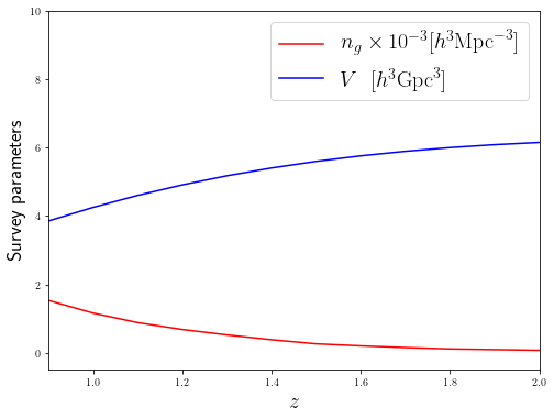
Figure 7: We show the mean galaxy number density and the survey volume. The survey covers about $0.38$ fraction of the sky and the redshift range of $0.9$ to $2.0$. This is the information used in estimating the SNR.

Appendix C Galaxy bispectrum: shape and anisotropic multipoles

C.1 Multipoles of the real space galaxy bispectrum

The galaxy density fluctuation $\delta_{g}$ is related to the matter density fluctuation $\delta_{m}$ according to the Eulerian bias model  [33, 34]

$$\delta_{\rm{g}}({\bm{r}})=b_{1}\delta_{m}({\bm{r}})+\frac{1}{2}\left[b_{2}\delta_{\rm{m}}({\bm{r}}))^{2}+b_{\mathcal{K}^{2}}\mathcal{K}^{2}({\bm{r}})\right]\,,$$ (C.1)

where $b_{1}$, $b_{2}$ and $b_{\mathcal{K}^{2}}$ are the linear, non-linear and tidal bias parameters respectively. $\mathcal{K}^{2}=\mathcal{K}_{ij}\mathcal{K}^{ij}$ is a scalar invariant tidal field constructed from the tidal tensor, At second order, we use the expression for the dark matter density field during the matter dominance

$$\delta^{\text{\tiny\color[rgb]{0,1,0}{({2}})}}({\bm{r}}) = \frac{34}{21}(\delta^{\text{\tiny\color[rgb]{1,0,0}{({1}})}})^{2}_{m}({\bm{r}})-2{\partial^{j}\nabla^{-2}\delta^{\text{\tiny\color[rgb]{1,0,0}{({1}})}}_{\rm{m}}}({\bm{r}})\partial_{j}\delta^{\text{\tiny\color[rgb]{1,0,0}{({1}})}}_{m}({\bm{r}})+\frac{4}{7}\mathcal{K}^{2}({\bm{r}})\,.$$ (C.2)

During the $\Lambda$CDM era, there are redshift dependent terms that appear in the coefficient of the terms above, however, equation (C.2) remains a good approximation [61]. In Fourier space $\delta_{g}({\bm{k}})=\delta_{g}^{\text{\tiny\color[rgb]{1,0,0}{({1}})}}({\bm{k}})+\delta_{g}^{\text{\tiny\color[rgb]{0,1,0}{({2}})}}({\bm{k}})$, with $\delta_{g}^{\text{\tiny\color[rgb]{1,0,0}{({1}})}}({\bm{k}})=b_{1}\delta_{m}^{\text{\tiny\color[rgb]{1,0,0}{({1}})}}({\bm{k}})$ and

$$\delta_{g}^{\text{\tiny\color[rgb]{0,1,0}{({2}})}}({\bm{k}}) = \int\frac{{d}^{3}k_{1}}{(2\pi)^{3}}\frac{{d}^{3}k_{2}}{(2\pi)^{3}}\delta_{m}({\bm{k}}_{1})\delta_{m}({\bm{k}}_{2})\mathcal{K}_{\rm{R}}^{(2)}({\bm{k}}_{1},{\bm{k}}_{2})(2\pi)^{3}\delta^{D}\left({\bm{k}}_{1}+{\bm{k}}_{2}-{\bm{k}}\right)\,,$$ (C.3)

where the second order momentum space kernel is given by

$$\mathcal{K}_{\rm{R}}^{(2)}(\bm{k}_{1},\bm{k}_{2}) = b_{2}+b_{1}F_{2}({\bm{k}}_{1},{\bm{k}}_{2})+b_{\mathcal{K}^{2}}\mathcal{K}_{2}({\bm{k}}_{1},{\bm{k}}_{2})\,,$$ (C.4)

where $F_{2}$ and $\mathcal{K}_{2}$ are the Fourier space kernel for the dark matter density and tidal field

$$F_{2}({\bm{k}}_{1},{\bm{k}}_{2}) = \frac{5}{7}+\frac{1}{2}\frac{{\bm{k}}_{1}\cdot{\bm{k}}_{2}}{k_{1}k_{2}}\left(\frac{k_{1}}{k_{2}}+\frac{k_{2}}{k_{1}}\right)+\frac{2}{7}\left(\frac{{\bm{k}}_{1}\cdot{\bm{k}}_{2}}{k_{1}k_{2}}\right)^{2}\,,$$ (C.5)

$$\mathcal{K}_{2}({\bm{k}}_{1},{\bm{k}}_{2}) = \frac{\left({\bm{k}}_{1}\cdot{\bm{k}}_{2}\right)^{2}}{\left(k_{1}k_{2}\right)^{2}}-\frac{1}{3}\,.$$ (C.6)

In perturbation theory, the tree level galaxy bispectrum may be calculated from two first order galaxy density constrast and one second order galaxy density contrast

$$\big{\langle}\delta_{g}(\bm{k}_{1})\delta_{g}(\bm{k}_{2})\delta_{g}(\bm{k}_{3})\big{\rangle} = \frac{1}{2}\big{\langle}\delta_{g}^{\text{\tiny\color[rgb]{1,0,0}{({1}})}}(\bm{k}_{1})\delta_{g}^{\text{\tiny\color[rgb]{1,0,0}{({1}})}}(\bm{k}_{2})\delta_{g}^{\text{\tiny\color[rgb]{0,1,0}{({2}})}}(\bm{k}_{3})\big{\rangle}+\text{2 cy. p.}$$ (C.7)

where we have included 2 clyic perturbation since the second order galaxy density contrast can occupy the first two slots as well. The real space galaxy bispectrum is given by

$$B_{g}({\bm{k}}_{1},{\bm{k}}_{2},{\bm{k}}_{3})=\mathcal{K}^{\text{\tiny\color[rgb]{0,1,0}{({2}})}}_{R}({\bm{k}}_{1},{\bm{k}}_{2})P_{m}(k_{1})P_{m}(k_{2})+\text{2 cy. p.}$$ (C.8)

where $P_{m}(k)$ is the matter power spectrum. We can expand the angular dependence of $B_{g}$ into Legendre polynomial

$$B_{g}({k}_{1},{k}_{2},\mu_{12}) = \sum_{\ell_{12}}B_{g\ell_{12}}({k}_{1},{k}_{2})\mathcal{L}_{\ell_{12}}(\mu_{12})\,,$$ (C.9)

Using the orthogonality condition we obtain the multipoles of the galaxy bispectrum

$$B_{g\ell_{12}}({k}_{1},{k}_{2}) = {{(2\ell_{12}+1)\over 2}}\int_{-1}^{1}{d}\mu_{12}B_{g}({k}_{1},{k}_{2},\mu_{12})\mathcal{L}_{\ell_{12}}(\mu_{12})\,.$$ (C.10)

C.2 Shape multipoles of the anisotropic galaxy bispectrum

Expanding equation (2.19) in Fourier space and in plane-parallel limit gives

$$\Delta_{\rm{N}}({\bm{k}}) = {\mathcal{K}}^{\text{\tiny\color[rgb]{1,0,0}{({1}})}}_{\rm{g}}({\bm{k}})\delta_{m}({\bm{k}})$$

$$+\frac{1}{2}\int\frac{d^{3}k_{1}}{(2\pi)^{3}}\frac{d^{3}k_{2}}{(2\pi)^{3}}{\mathcal{K}_{\rm{g}}}^{\text{\tiny\color[rgb]{0,1,0}{({2}})}}({\bm{k}}_{1},{\bm{k}}_{2},{\bm{k}}_{3})\delta_{m}({\bm{k}}_{1})\delta_{m}({\bm{k}}_{2})(2\pi)^{3}\delta^{(3)}\left({\bm{k}}-{\bm{k}}_{1}-{\bm{k}}_{2}\right)\,.$$

where $\mathcal{K}_{\rm{N}}$ is a Fourier space kernel for the galaxy density in redshift space, we have separated $\mathcal{K}_{\rm{N}}$ into linear and the second order part gives

$$\mathcal{K}_{\rm{N}}^{\text{\tiny\color[rgb]{1,0,0}{({1}})}}(k_{1}) = b_{1}+f\mu^{2}_{1}\,,$$ (C.12)

$$\mathcal{K}_{\rm{N}}^{\text{\tiny\color[rgb]{0,1,0}{({2}})}}(\bm{k}_{1},\bm{k}_{2},\bm{k}_{3}) = b_{2}+b_{1}F_{2}({\bm{k}}_{1},{\bm{k}}_{2})+b_{\mathcal{K}^{2}}\mathcal{K}_{2}({\bm{k}}_{1},{\bm{k}}_{2})+f\,G_{2}({\bm{k}}_{1},{\bm{k}}_{2})\mu_{3}^{2}+{\cal Z}_{2}({\bm{k}}_{1},{\bm{k}}_{2})\,,$$ (C.13)

Here we decompose each ${\bm{k}}$ with respect to ${{\bf\hat{n}}}$; ${k}_{M}^{i}={k}_{M\|}n^{i}+{k}_{\bot M}^{i}=\mu_{M}k_{M}n^{i}+{k}_{\bot M}^{i}$, where ${k}_{M\|}$ is the parallel component ${k}_{M\|}={k}_{M}^{i}{n}_{i}=\mu_{M}k_{M}$ and ${k}_{\bot M}^{i}$ is the transverse component ${k}_{\bot M}^{i}{n}^{i}=0$ and $\mu_{M}={\hat{\bm{k}}_{M}\cdot{{\bf\hat{n}}}}$. ${\cal Z}_{2}$ is a collection of the second order biased-dependent redshift space distortion terms [62]

$${\cal Z}_{2}(\bm{k}_{1},\bm{k}_{2}) = (f\mu_{3}k_{3})\left[\frac{\mu_{1}}{k_{1}}\left(b_{1}+f\mu^{2}_{2}\right)+\frac{\mu_{2}}{k_{2}}\left(b_{1}+f\mu^{2}_{1}\right)\right]\,,$$ (C.14)

where ${\bm{k}}_{3}\equiv{\bm{k}}_{1}+{\bm{k}}_{2}$. Furthermore, we made use of the Euler equation to relate the peculiar velocity to the matter density contrast

$$v({\bm{k}}) = \frac{\mathcal{H}f}{k^{2}}\left[\delta_{m}^{\text{\tiny\color[rgb]{1,0,0}{({1}})}}({\bm{k}})+\int\frac{{d}^{3}k_{1}}{(2\pi)^{3}}\frac{{d}^{3}k_{2}}{(2\pi)^{3}}\delta_{m}({\bm{k}}_{1})\delta_{m}({\bm{k}}_{2})G_{2}({\bm{k}}_{1},{\bm{k}}_{2})(2\pi)^{3}\delta^{D}\left({\bm{k}}_{1}+{\bm{k}}_{2}-{\bm{k}}\right)\right]\,,$$ (C.15)

where $G_{2}$ are the kernel for the dark matter density field and the peculiar velocity kernel at second order respectively:

$$G_{2}({\bm{k}}_{1},{\bm{k}}_{2}) = \frac{3}{7}+\frac{1}{2}\frac{{\bm{k}}_{1}\cdot{\bm{k}}_{2}}{k_{1}k_{2}}\left(\frac{k_{1}}{k_{2}}+\frac{k_{2}}{k_{1}}\right)+\frac{4}{7}\left(\frac{{\bm{k}}_{1}\cdot{\bm{k}}_{2}}{k_{1}k_{2}}\right)^{2}\,,$$ (C.16)

The galaxy bispectrum is given by [16, 62]

$$B_{g}({\bm{k}}_{1},{\bm{k}}_{2},{\bm{k}}_{3})=\mathcal{K}_{\rm{N}}^{\text{\tiny\color[rgb]{1,0,0}{({1}})}}({\bm{k}}_{1})\mathcal{K}_{{\rm{N}}}^{\text{\tiny\color[rgb]{1,0,0}{({1}})}}({\bm{k}}_{2})\mathcal{K}_{\rm{N}}^{\text{\tiny\color[rgb]{0,1,0}{({2}})}}({\bm{k}}_{1},{\bm{k}}_{2},{\bm{k}}_{3})P_{m}(k_{1})P_{m}(k_{2})+\text{2 cy. p.}$$ (C.17)

where $P_{m}(k)$ is the matter power spectrum. $B_{g}$ depends on nine free parameters, in the real space limit, one can impose the homogeneity and isotropy of the triangular configurations to reduce the nine free parameters to three; magnitude of the two sides and the angle between them. In redshift, the map in equation (2.18) introduces a unique line of sight which breaks isotropy. Using the closure relation (translation invariance) for the closed triangle ${\bm{k}}_{1}+{\bm{k}}_{2}+{\bm{k}}_{3}=0$, the number of free variables maybe reduced to six, this implies that we can fix $\mu_{3}$ using $\mu_{1}k_{1}+\mu_{2}k_{2}+\mu_{3}k_{3}=0$ and $k_{3}$ in terms of $k_{1}$, $k_{2}$ and the angle between them $\mu_{12}$. Using the trigonometric identity, $\mu_{2}$ may be expressed in terms of $\mu_{1}$ and the azimuthal angle $\phi_{n}$

$$\mu_{2} = \mu_{1}\mu_{12}\pm\sqrt{1-\mu_{1}^{2}}\sqrt{1-\mu_{12}^{2}}\cos\phi_{n}\,,$$ (C.18)

$$\mu_{3} = -\frac{k_{1}}{k_{3}}\mu_{1}-\frac{k_{2}}{k_{3}}\mu_{2}\,.$$ (C.19)

where $\mu_{12}={\hat{\bm{k}}_{1}\cdot\hat{\bm{k}}_{2}}$ is the angle between ${\bm{k}}_{1}$ and ${\bm{k}}_{2}$. This decomposition which reduces the number of free parameters from nine to five, is the most optimal decomposition of the galaxy bispectrum in redshift space, $B_{g}({k}_{1},{k}_{2},\mu_{12},\mu_{1},\phi_{n})$ and was first introduced in [43, 15].

We shall go slightly higher to reduce the number of free parameters from five to four by averaging over the dependence on azimuthal angle to obtain the so-called $\phi_{n}$-average galaxy bispectrum

$$B_{g}^{\phi_{n}}({k}_{1},{k}_{2},\mu_{12},\mu_{1})\equiv\frac{1}{2\pi}\int_{0}^{2\pi}{d}\phi_{n}B_{g}({k}_{1},{k}_{2},\mu_{12},\mu_{1},\phi_{n})\,$$ (C.20)

It helps to reduce the dimensionality of the data structures of the bispectrum measurements. For a fixed cosmological model, the loss of information has been shown to be very small [45]. In this limit, the spherical harmonics ${Y_{L}^{M}}$ reduces to the Legendre polynominial. Expanding $\mu_{12}$ in Legendre polynomial as well leads to

$$B_{g}^{\phi_{n}}({k}_{1},{k}_{2},\mu_{12},\mu_{1}) = \sum_{L=0}^{\infty}\sum_{\ell_{12}}B^{\phi_{n}}_{gL\ell_{12}}({k}_{1},{k}_{2})\mathcal{L}_{\ell_{12}}(\mu_{12})\mathcal{L}_{L}(\mu_{1})\,,$$ (C.21)

Using the orthogonality condition we obtain the multipole moments with respect to $L$ and $\ell_{12}$ of the galaxy bispectrum

$$B_{gL\ell_{12}}^{\rm{N}\phi_{n}}({k}_{1},{k}_{2}) = {{(2\ell_{12}+1)\over 2}}{{(2L+1)\over 2}}\int_{-1}^{1}{d}\mu_{1}\int_{-1}^{1}{d}\mu_{12}\,$$

$$\qquad\qquad~{}~{}~{}~{}~{}~{}~{}\times~{}B_{g}^{\rm{N}\phi_{n}}({k}_{1},{k}_{2},\mu_{12},\mu_{1})\mathcal{L}_{\ell_{12}}(\mu_{12})\mathcal{L}_{L}(\mu_{1})\,.$$

If one chooses to count the number of triangles instead of decomposing the angle between ${\bm{k}}_{1}$ and ${\bm{k}}_{2}$ into multipoles, summing over the first few multipoles of order $\ell_{12}$ will recover $B_{gL\lambda}$ provided $B_{g}$ is a well behaved function of its other argurments.

Appendix D More details on the technical derivation

D.1 Details on the derivation of 3PCF

We use the spherical harmonics addition theorem

$$\mathcal{L}_{\ell}(\nu_{13})=\frac{4\pi}{(2\ell+1)}\sum_{m=-\ell}^{\ell}Y^{\ast}_{\ell m}(\hat{\bm{r}}_{13})Y_{\ell m}(\hat{\bm{r}}_{23})=\frac{4\pi}{(2\ell+1)}\sum_{m=-\ell}^{\ell}Y_{\ell m}(\hat{\bm{r}}_{13})Y^{\ast}_{\ell m}(\hat{\bm{r}}_{23})$$ (D.1)

to express the Legendre polynomials in the spherical harmonics basis. The product of spherical harmonics is given by

$$Y_{\ell_{1},m_{1}}({\bm{r}}_{13})Y_{\ell_{2},m_{2}}({\bm{r}}_{13}) = \sum_{m_{3}=-\ell_{3}}^{m_{3}=\ell_{3}}\sum_{\ell_{3}=|\ell_{1}-\ell_{2}|}^{\ell_{1}+\ell_{2}}\left({\begin{array}[]{ccc}\ell_{1}&\ell_{2}&\ell_{3}\\ m_{1}&{m_{2}}&m_{3}\\ \end{array}}\right)\mathcal{H}_{\ell_{1},\ell_{2},\ell_{3}}^{0,0,0}Y_{\ell_{3}m_{3}}({\bm{r}}_{13})\,,$$ (D.4)

where we have separated $\mathcal{G}_{\ell_{1}\ell_{2}\ell_{3}}^{m_{1}m_{2}m}$ into m-dependent 3j symbol and

$$\mathcal{H}_{\ell_{1}\ell_{2}\ell_{3}}^{0,0,0} = \sqrt{\frac{(2\ell_{1}+1)(2\ell_{2}+1)(2\ell_{3}+1)}{4\pi}}\begin{pmatrix}\ell_{1}&\ell_{2}&\ell_{3}\\ 0&0&0\end{pmatrix}\,.$$ (D.5)

Putting the multipole expansion of $B_{g}^{\phi_{n}}$ in equation (2.20) gives

$$\zeta_{g}({\bm{r}}_{13},{\bm{r}}_{23},{{\bf\hat{n}}}) = \sum_{\ell_{1},\ell_{2}L\ell_{12}}{(2\ell_{1}+1)(2\ell_{2}+1)}i^{\ell_{1}+\ell_{2}}\int\frac{{d}k_{1}k^{2}_{1}}{(2\pi)^{3}}\int\frac{{d}k_{2}k^{2}_{2}}{(2\pi)^{3}}\int{d}{\bm{k}}_{{\bot}_{1}}\int{d}{\bm{k}}_{{\bot}_{2}}j_{\ell_{1}}(k_{1}r_{13})$$ (D.6)

$$\times j_{\ell_{2}}(k_{2}r_{23})B^{\phi_{n}}_{gL\ell_{12}}({k}_{1},{k}_{2})\mathcal{L}_{\ell_{12}}(\hat{\bm{k}}_{1}\cdot\hat{\bm{k}}_{2})\mathcal{L}_{L}({\hat{\bm{k}}}_{1}\cdot{{\bf\hat{n}}})\ \mathcal{L}_{\ell_{1}}({\hat{\bm{r}}}_{13}\cdot{\hat{\bm{k}}}_{1})\mathcal{L}_{\ell_{2}}({\hat{\bm{r}}}_{23}\cdot{\hat{\bm{k}}}_{2})\,,$$

We made use of equation (D.1) to express the Legendre polynomial in terms of the spherical harmonics

$$\mathcal{L}_{\ell_{12}}({\bm{k}}_{1}\cdot{\bm{k}}_{2})\mathcal{L}_{L}({\bm{k}}_{1}\cdot{{\bf\hat{n}}})\mathcal{L}_{\ell_{1}}({{\bm{r}}_{13}}\cdot{{\bm{k}}_{1}})\mathcal{L}_{\ell_{2}}({{\bm{r}}_{23}}\cdot{{\bm{k}}_{2}})$$

$$= \frac{4\pi}{(2\ell_{1}+1)}\frac{4\pi}{(2\ell_{2}+1)}\frac{4\pi}{(2\ell_{12}+1)}\frac{4\pi}{(2L+1)}\sum_{m=-\ell_{1}}^{\ell_{1}}\sum_{m=-\ell_{2}}^{\ell_{2}}\sum_{m=-\ell_{12}}^{\ell_{12}}\sum_{m=-L}^{L}$$

$$\times Y_{\ell_{1}m_{1}}^{\ast}({{\bm{r}}}_{13})Y_{\ell_{2}m_{2}}({{\bm{r}}}_{23})Y_{LM}({{\bf\hat{n}}})Y_{\ell_{1}m_{1}}({\bm{k}}_{1})Y^{\ast}_{\ell_{12}m_{12}}({\bm{k}}_{1})Y^{\ast}_{LM}({\bm{k}}_{1})Y^{\ast}_{\ell_{2}m_{2}}({\bm{k}}_{2})Y_{\ell_{12}m_{12}}({\bm{k}}_{2})\,.$$

Then performed the $\hat{\bm{k}}_{2}$ and $\hat{\bm{k}}_{1}$ using

$$\int d\Omega_{k_{2}}Y_{\ell_{2}m_{2}}({\bm{k}}_{2})Y^{*}_{\ell_{12}m_{12}}({\bm{k}}_{2}) = \delta_{\ell_{2}\ell_{12}}\delta_{m_{2}m_{12}}\,,$$ (D.8)

$$\quad\int d^{2}{{\hat{\bm{k}}_{1}}}Y^{\star}_{\ell_{1}m_{1}}({{\hat{\bm{k}}_{1}}})Y^{\star}_{\ell_{12}m_{12}}({{\hat{\bm{k}}_{1}}})Y_{LM}({{\hat{\bm{k}}_{1}}}) = \begin{pmatrix}\ell_{12}&L&\ell_{1}\\ m_{12}&M&m_{1}\end{pmatrix}\mathcal{H}_{\ell_{12}L\ell_{1}}^{0,0,0}\,.$$ (D.9)

After performing the Kronecker delta summation and some algebraic simplification we find

$$\zeta_{g}({\bm{r}}_{13},{\bm{r}}_{23},{{\bf\hat{n}}}) = \sum_{{L}\ell_{1}\ell_{12}}\sum_{m_{1}m_{12}M}\frac{4\pi}{(2\ell_{12}+1)}\frac{4\pi}{(2L+1)}\int\frac{{d}k_{1}k^{2}_{1}}{2\pi^{2}}\int\frac{{d}k_{2}k^{2}_{2}}{2\pi^{2}}i^{\ell_{1}+\ell_{12}}\mathcal{G}_{\ell_{1}\ell_{12}L}^{m_{1}m_{12}M}$$ (D.10)

$$\times B_{\text{g}\ell_{12}L}^{\phi_{n}}(z,k_{1},k_{2})j_{\ell_{1}}(k_{1}r_{13})j_{\ell_{12}}(k_{2}r_{23})Y_{\ell_{1}m_{1}}^{\ast}({\hat{\bm{r}}}_{13})Y_{\ell_{12}m_{12}}(\hat{\bf{r}}_{23})Y_{LM}({{\bf\hat{n}}})\,,$$

Substituting equation (D.10) in equation (2.29) gives

$${\zeta}^{\phi_{n}}_{L\ell_{12}}({r}_{13},{r}_{23}) = i^{\ell_{3}+\ell_{12}}\int_{0}^{\infty}\frac{{d}k_{1}k^{2}_{1}}{2\pi^{2}}\int_{0}^{\infty}\frac{{d}k_{2}k^{2}_{2}}{2\pi^{2}}B_{{g}L\ell_{12}}(k_{1},k_{2})j_{\ell_{3}}(k_{1}r_{12})j_{\ell_{12}}(k_{2}r_{23})\,.$$ (D.11)

D.2 Details on the derivation of 3PCF covariance

We make use of the plane wave approximation

$$e^{i{\bm{k}}_{1}\cdot{\bm{r}}_{13}} = \sum_{\ell_{3}}(2\ell_{3}+1)i^{\ell_{3}}j_{\ell_{3}}(kr_{13})\mathcal{L}_{\ell_{3}}(\hat{\bf{r}}_{13}\cdot\hat{{\bm{k}}_{1}})\,,$$ (D.12)

$$e^{i{\bm{k}}_{2}\cdot{\bm{r}}_{23}} = \sum_{\ell_{3}}(2\ell_{3}+1)i^{\ell_{3}}j_{\ell_{3}}(k_{2}r_{23})\mathcal{L}_{\ell_{3}}(\hat{{\bm{r}}}_{23}\cdot\hat{\bm{k}}_{2})\,.$$ (D.13)

Substituting these in equation (3) and performing some algebraic simplification leads to

$${\rm{Cov}}\left[\hat{\zeta}_{g}({\bm{r}}_{13},{\bm{r}}_{23},{{\bf\hat{n}}})\hat{\zeta}_{g}({\bm{r}}^{\prime}_{13},{\bm{r}}^{\prime}_{23},{{\bf\hat{n}}})\right] = \int{{d}k_{1}}k_{1}^{2}\int{{d}k_{2}}k_{2}^{2}\int{d}^{2}{\bm{k}}_{1}\int{d}^{2}{\bm{k}}_{2}\sum_{L_{2}\ell_{12}}\frac{\left(P({k}_{1})P({k}_{2})P({k}_{12})\right)_{L_{2}\ell_{12}}}{(2\pi)^{6}V_{s}}$$ (D.14)

$$\sum_{\ell_{1}\ell_{1}^{\prime}}\sum_{\ell_{2}\ell_{2}^{\prime}}(2\ell_{1}+1)(2\ell_{1}^{\prime}+1)(2\ell_{2}+1)(2\ell_{2}^{\prime}+1)(i)^{\ell_{1}+\ell_{2}}(-i)^{\ell_{1}^{\prime}+\ell_{2}^{\prime}}$$

$$\bigg{[}j_{\ell_{1}}(k_{1}r_{13})j_{\ell_{1}^{\prime}}(k_{1}r^{\prime}_{13})j_{\ell_{2}}(k_{2}r_{23})j_{\ell_{2}^{\prime}}(k_{2}r^{\prime}_{23})$$

$$\times X^{1}_{\ell_{1}\ell_{1}^{\prime}\ell_{2}\ell_{2}^{\prime}L_{2}\ell_{12}}([\hat{\bm{k}}_{1},\hat{\bm{r}}_{13},\hat{\bm{r}}^{\prime}_{13}],[\hat{\bm{k}}_{2},\hat{\bm{r}}_{23},\hat{\bm{r}}^{\prime}_{23}],{{\bf\hat{n}}})$$

$$+j_{\ell_{1}}(k_{1}r_{13})j_{\ell_{1}^{\prime}}(k_{1}r^{\prime}_{23})j_{\ell_{2}}(k_{2}r_{23})j_{\ell_{2}^{\prime}}(k_{2}r^{\prime}_{13})$$

$$\times X^{2}_{\ell_{1}\ell_{1}^{\prime}\ell_{2}\ell_{2}^{\prime}L_{2}\ell_{12}}([\hat{\bm{k}}_{1},\hat{\bm{r}}_{13},\hat{\bm{r}}^{\prime}_{23}],[\hat{\bm{k}}_{2},\hat{\bm{r}}_{23},\hat{\bm{r}}^{\prime}_{13}],{{\bf\hat{n}}})\bigg{]}\,,$$

where

$$X^{1}_{\ell_{1}\ell_{1}^{\prime}\ell_{2}\ell_{2}^{\prime}L\ell_{12}}([\hat{\bm{k}}_{1},\hat{\bm{r}}_{13},\hat{\bm{r}}^{\prime}_{13}],[\hat{\bm{k}}_{2},\hat{\bm{r}}_{23},\hat{\bm{r}}^{\prime}_{23}],{{\bf\hat{n}}}) = \mathcal{L}_{\ell_{1}}(\hat{{\bm{r}}}_{13}\cdot\hat{{\bm{k}}_{1}})\mathcal{L}_{\ell_{1}^{\prime}}(\hat{{\bm{r}}^{\prime}}_{13}\cdot\hat{{\bm{k}}}_{1})\mathcal{L}_{\ell_{2}}(\hat{{\bm{r}}}_{23}\cdot\hat{\bm{k}}_{2})$$

$$\mathcal{L}_{\ell_{2}^{\prime}}(\hat{\bm{r}}^{\prime}_{23}\cdot\hat{\bm{k}}_{2})\mathcal{L}_{L}({\bm{k}}_{1}\cdot{{\bf\hat{n}}})\mathcal{L}_{\ell_{12}}({\bm{k}}_{1}\cdot{\bm{k}}_{2})\,,$$

$$X^{2}_{\ell_{1}\ell_{1}^{\prime}\ell_{2}\ell_{2}^{\prime}L_{2}\ell_{12}}([\hat{\bm{k}}_{1},\hat{\bm{r}}_{13},\hat{\bm{r}}^{\prime}_{23}],[\hat{\bm{k}}_{2},\hat{\bm{r}}_{23},\hat{\bm{r}}^{\prime}_{13}],{{\bf\hat{n}}}) = \mathcal{L}_{\ell_{1}}(\hat{{\bm{r}}}_{13}\cdot\hat{{\bm{k}}_{1}})\mathcal{L}_{\ell_{1}^{\prime}}(\hat{{\bm{r}}^{\prime}}_{23}\cdot\hat{{\bm{k}}_{1}})\mathcal{L}_{\ell_{2}}(\hat{{\bm{r}}}_{23}\cdot\hat{{\bm{k}}_{2}})$$

$$\mathcal{L}_{\ell_{2}^{\prime}}(\hat{{\bm{r}}^{\prime}}_{13}\cdot\hat{{\bm{k}}_{2}})\mathcal{L}_{L_{2}}({\bm{k}}_{1}\cdot{{\bf\hat{n}}})\mathcal{L}_{\ell_{12}}({\bm{k}}_{1}\cdot{\bm{k}}_{2})\,.$$

Putting equation (D.14) in equation (3) leads to

$${\rm{Cov}}\left[\hat{\zeta}^{\phi_{n}}_{\ell_{13}L}({r}_{13},{r}_{23})\hat{\zeta}^{\phi_{n}}_{\ell^{\prime}_{13}L^{\prime}}({r}^{\prime}_{13},{r}^{\prime}_{23})\right] = \bigg{[}\frac{(2L+1)(2\ell_{13}+1)}{\mathcal{L}_{\ell_{12},L,\ell_{3}}}\frac{{{(2L^{\prime}+1)}}(2\ell^{\prime}_{13}+1)}{\mathcal{L}_{\ell^{\prime}_{13},L^{\prime},\ell^{\prime}_{3}}}\bigg{]}$$

$$\sum_{m_{13}Mm_{3}}\left({\begin{array}[]{ccc}\ell_{13}&L&\ell_{3}\\ m_{13}&{M}&m_{3}\\ \end{array}}\right)\sum_{m^{\prime}_{13}M^{\prime}m^{\prime}_{3}}\left({\begin{array}[]{ccc}\ell^{\prime}_{13}&L^{\prime}&\ell^{\prime}_{3}\\ m^{\prime}_{13}&{M^{\prime}}&m^{\prime}_{3}\\ \end{array}}\right)$$

$$\int{{d}k_{1}}k_{1}^{2}\int{{d}k_{2}}k_{2}^{2}\sum_{L_{2}\ell_{12}}\frac{\left(P({k}_{1})P({k}_{2})P({k}_{12})\right)_{L_{2}\ell_{12}}}{(V_{s})2\pi)^{6}}$$

$$\sum_{\ell_{1}\ell_{1}^{\prime}}\sum_{\ell_{2}\ell_{2}^{\prime}}(2\ell_{1}+1)(2\ell_{1}^{\prime}+1)(2\ell_{2}+1)(2\ell_{2}^{\prime}+1)(i)^{\ell_{1}+\ell_{2}}(-i)^{\ell_{1}^{\prime}+\ell_{2}^{\prime}}$$

$$\int\mathrm{d}^{2}\mathbf{r}_{13}\int\mathrm{d}^{2}\mathbf{r}_{23}\int\mathrm{d}^{2}\mathbf{r}^{\prime}_{13}\int\mathrm{d}^{2}\mathbf{r}^{\prime}_{23}\int{d}^{2}{{\bf\hat{n}}}\int{d}^{2}{\bm{k}}_{1}\int{d}^{2}{\bm{k}}_{2}$$

$$\bigg{[}j_{\ell_{1}}(k_{1}r_{13})j_{\ell_{1}^{\prime}}(k_{1}r^{\prime}_{13})j_{\ell_{2}}(k_{2}r_{23})j_{\ell_{2}^{\prime}}(k_{2}r^{\prime}_{23})$$

$$X^{1}_{\ell_{1}\ell_{1}^{\prime}\ell_{2}\ell_{2}^{\prime}L_{2}\ell_{12}}([\hat{\bm{k}}_{1},\hat{\bm{r}}_{13},\hat{\bm{r}}^{\prime}_{13}],[\hat{\bm{k}}_{2},\hat{\bm{r}}_{23},\hat{\bm{r}}^{\prime}_{23}],{{\bf\hat{n}}})$$

$$+j_{\ell_{1}}(k_{1}r_{13})j_{\ell_{1}^{\prime}}(k_{1}r^{\prime}_{23})j_{\ell_{2}}(k_{2}r_{23})j_{\ell_{2}^{\prime}}(k_{2}r^{\prime}_{13})$$

$$X^{2}_{\ell_{1}\ell_{1}^{\prime}\ell_{2}\ell_{2}^{\prime}L_{2}\ell_{12}}([\hat{\bm{k}}_{1},\hat{\bm{r}}_{13},\hat{\bm{r}}^{\prime}_{23}],[\hat{\bm{k}}_{2},\hat{\bm{r}}_{23},\hat{\bm{r}}^{\prime}_{13}],{{\bf\hat{n}}})\bigg{]}$$

$$\times\mathcal{Y}_{\ell_{3}\ell_{13}L}^{m_{3}m_{13}M}(\hat{\bm{r}}_{13},\hat{\bm{r}}_{23},{{\bf\hat{n}}})\mathcal{Y}_{\ell^{\prime}_{3}\ell^{\prime}_{13}L^{\prime}}^{m^{\prime}_{3}m^{\prime}_{13}M^{\prime}}(\hat{\bm{r}}^{\prime}_{13},\hat{\bm{r}}^{\prime}_{23},{{\bf\hat{n}}}^{\prime})\,,$$

where

$$\mathcal{Y}_{\ell_{3}\ell_{13}L}^{m_{3}m_{13}M}(\hat{\bm{r}}_{13},\hat{\bm{r}}_{23},{{\bf\hat{n}}}) = \left[Y^{\ast}_{\ell_{3}m_{3}}(\hat{\bm{r}}_{13})Y^{\ast}_{\ell_{13}m_{13}}(\hat{\bm{r}}_{23})Y_{LM}({{\bf\hat{n}}})\right]\,.$$ (D.22)

Using the addition theorem, we can express the Legendre polynomial in terms of the spherical harmonics

$$X^{1}_{\ell_{1}\ell_{1}^{\prime}\ell_{2}\ell_{2}^{\prime}L\ell_{12}}([\hat{\bm{k}}_{1},\hat{\bm{r}}_{13},\hat{\bm{r}}^{\prime}_{13}],[\hat{\bm{k}}_{2},\hat{\bm{r}}_{23},\hat{\bm{r}}^{\prime}_{23}],{{\bf\hat{n}}}) = \frac{4\pi}{(2\ell_{1}+1)}\frac{4\pi}{(2\ell_{1}^{\prime}+1)}\frac{4\pi}{(2\ell_{2}+1)}\frac{4\pi}{(2\ell_{2}^{\prime}+1)}\frac{4\pi}{(2L_{2}+1)}\frac{4\pi}{(2\ell_{12}+1)}$$

$$\sum_{m_{1}=-\ell_{1}}^{\ell_{1}}\sum_{m_{1}^{\prime}=-\ell_{1}}^{\ell_{1}^{\prime}}\sum_{m_{2}=-\ell_{2}}^{\ell_{2}}\sum_{m_{2}^{\prime}=-\ell_{2}}^{\ell_{2}^{\prime}}\sum_{m_{12}=-\ell_{12}}^{\ell_{12}}\sum_{M_{2}=-L_{2}}^{L_{2}}$$

$$Y_{\ell_{1}m_{1}}(\hat{\bm{r}}_{13})Y_{\ell_{1}^{\prime}m_{1}^{\prime}}(\hat{\bm{r}}^{\prime}_{13})$$

$$Y_{\ell_{2}m_{2}}\hat{(}{\bm{r}}_{23})Y_{\ell_{2}^{\prime}m_{2}^{\prime}}\hat{(}{\bm{r}}^{\prime}_{23})$$

$$Y^{\ast}_{\ell_{12}m_{12}}(\hat{\bm{k}}_{1})Y_{L_{2}M_{2}}(\hat{\bm{k}}_{1})Y^{\ast}_{\ell_{1}m_{1}}(\hat{\bm{k}}_{1})Y^{\ast}_{\ell_{1}^{\prime}m_{1}^{\prime}}(\hat{\bm{k}}_{1})$$

$$Y^{\ast}_{\ell_{2}^{\prime}m_{2}^{\prime}}(\hat{\bm{k}}_{2})Y^{\ast}_{\ell_{2}m_{2}}(\hat{\bm{k}}_{2})Y_{\ell_{12}m_{12}}(\hat{\bm{k}}_{2})$$

$$Y^{\ast}_{L_{2}M_{2}}({{\bf\hat{n}}})\,.$$

Note that $Y_{\ell m}^{\ast}=(-1)^{m}Y_{\ell-m}$. Using equation (D.2), we can not perform the angular integrals using equation (D.8), (D.9) and

$$\int{d}^{2}{\bm{k}}_{1}Y^{\ast}_{\ell_{12}m_{12}}({\bm{k}}_{1})Y_{L_{2}M_{2}}({\bm{k}}_{1})Y^{\ast}_{\ell_{1}m_{1}}({\bm{k}}_{1})Y^{\ast}_{\ell_{1}^{\prime}m_{1}^{\prime}}({\bm{k}}_{1})$$

$$= \sum_{M_{3}=-L_{3}}^{M_{3}=L_{3}}\sum_{L_{3}=|\ell_{1}-\ell_{1}^{\prime}|}^{\ell_{1}+\ell_{1}^{\prime}}\begin{pmatrix}L_{2}&\ell_{12}&L_{3}\\ M_{2}&m_{12}&M_{3}\end{pmatrix}\begin{pmatrix}\ell_{1}&\ell^{\prime}_{1}&L_{3}\\ m_{1}&m^{\prime}_{1}&M_{3}\end{pmatrix}\mathcal{L}_{L_{2}\ell_{12}L_{3}}^{0,0,0}\mathcal{L}_{\ell_{1}\ell^{\prime}_{1}L_{3}}^{0,0,0}\,.$$

Performing $\ell_{1}$ and $\ell_{2}$ sums and $\ell^{\prime}_{1}$ and $\ell^{\prime}_{2}$ sums and using the following definition of the 9j symbol

$$\sum_{m_{13}Mm_{3}}\sum_{m^{\prime}_{13}M^{\prime}m^{\prime}_{3}}\sum_{m_{12}M_{2}M_{3}}\left({\begin{array}[]{ccc}\ell_{13}&L&\ell_{3}\\ m_{13}&M&m_{3}\\ \end{array}}\right)\left({\begin{array}[]{ccc}\ell^{\prime}_{13}&L^{\prime}&\ell^{\prime}_{3}\\ m^{\prime}_{13}&M^{\prime}&m^{\prime}_{3}\\ \end{array}}\right)\begin{pmatrix}\ell_{12}&L_{2}&L_{3}\\ m_{12}&M_{2}&M_{3}\end{pmatrix}$$ (D.29)

$$\begin{pmatrix}\ell_{3}&\ell^{\prime}_{3}&L_{3}\\ m_{3}&m^{\prime}_{3}&M_{3}\end{pmatrix}\begin{pmatrix}\ell_{13}&\ell^{\prime}_{13}&\ell_{12}\\ m_{13}&m^{\prime}_{13}&m_{12}\end{pmatrix}\begin{pmatrix}L&L^{\prime}&L_{2}\\ M&M^{\prime}&M_{2}\end{pmatrix}=\begin{Bmatrix}\ell_{13}&L&\ell_{3}\\ \ell^{\prime}_{13}&L^{\prime}&\ell^{\prime}_{3}\\ \ell_{12}&L_{2}&L_{3}\end{Bmatrix}\,,$$

lead to equation (3). Note that simplification of

$$X^{2}_{\ell_{1}\ell_{1}^{\prime}\ell_{2}\ell_{2}^{\prime}L_{2}\ell_{12}}([{\bm{k}}_{1},{\bm{r}}_{13},{\bm{r}}^{\prime}_{23}],[{\bm{k}}_{2},{\bm{r}}_{23},{\bm{r}}^{\prime}_{13}],{{\bf\hat{n}}}) = \mathcal{L}_{\ell_{1}}(\hat{{\bm{r}}}_{13}\cdot\hat{{\bm{k}}_{1}})\mathcal{L}_{\ell_{1}^{\prime}}(\hat{{\bm{r}}^{\prime}}_{23}\cdot\hat{{\bm{k}}_{1}})\mathcal{L}_{\ell_{2}}(\hat{{\bm{r}}}_{23}\cdot\hat{{\bm{k}}_{2}})$$

$$\mathcal{L}_{\ell_{2}^{\prime}}(\hat{{\bm{r}}^{\prime}}_{13}\cdot\hat{{\bm{k}}_{2}})\mathcal{L}_{L_{2}}({\bm{k}}_{1}\cdot{{\bf\hat{n}}})\mathcal{L}_{\ell_{12}}({\bm{k}}_{1}\cdot{\bm{k}}_{2})\,,$$

follows the same procedure.

References

- [1] H. Gil-Marín, J. Noreña, L. Verde, W. J. Percival, C. Wagner, M. Manera, and D. P. Schneider, The power spectrum and bispectrum of SDSS DR11 BOSS galaxies – I. Bias and gravity, Mon. Not. Roy. Astron. Soc. 451 (2015), no. 1 539–580, [arXiv:1407.5668].
- [2] N. Bartolo, E. Komatsu, S. Matarrese, and A. Riotto, Non-Gaussianity from inflation: Theory and observations, Phys. Rept. 402 (2004) 103–266, [astro-ph/0406398].
- [3] P. Creminelli and M. Zaldarriaga, CMB 3-point functions generated by non-linearities at recombination, Phys. Rev. D70 (2004) 083532, [astro-ph/0405428].
- [4] P. Creminelli, J. Gleyzes, L. Hui, M. Simonovi, and F. Vernizzi, Single-Field Consistency Relations of Large Scale Structure. Part III: Test of the Equivalence Principle, JCAP 1406 (2014) 009, [arXiv:1312.6074].
- [5] X. Chen, M.-x. Huang, S. Kachru, and G. Shiu, Observational signatures and non-Gaussianities of general single field inflation, JCAP 01 (2007) 002, [hep-th/0605045].
- [6] R. Scoccimarro, L. Hui, M. Manera, and K. C. Chan, Large-scale Bias and Efficient Generation of Initial Conditions for Non-Local Primordial Non-Gaussianity, Phys.Rev. D85 (2012) 083002, [arXiv:1108.5512].
- [7] N. Arkani-Hamed and J. Maldacena, Cosmological Collider Physics, arXiv:1503.08043.
- [8] Z. Slepian and D. J. Eisenstein, Computing the three-point correlation function of galaxies in time, Mon. Not. Roy. Astron. Soc. 454 (2015), no. 4 4142–4158, [arXiv:1506.02040].
- [9] I. Szapudi, Three - point statistics from a new perspective, Astrophys. J. 605 (2004) L89, [astro-ph/0404476].
- [10] Z. Slepian et al., Detection of baryon acoustic oscillation features in the large-scale three-point correlation function of SDSS BOSS DR12 CMASS galaxies, Mon. Not. Roy. Astron. Soc. 469 (2017), no. 2 1738–1751, [arXiv:1607.06097].
- [11] Z. Slepian and D. J. Eisenstein, Modelling the large-scale redshift-space 3-point correlation function of galaxies, Mon. Not. Roy. Astron. Soc. 469 (2017), no. 2 2059–2076, [arXiv:1607.03109].
- [12] Z. Slepian and D. J. Eisenstein, A practical computational method for the anisotropic redshift-space three-point correlation function, Mon. Not. Roy. Astron. Soc. 478 (2018), no. 2 1468–1483, [arXiv:1709.10150].
- [13] B. Friesen et al., Galactos: Computing the Anisotropic 3-Point Correlation Function for 2 Billion Galaxies, arXiv:1709.00086.
- [14] R. Scoccimarro, S. Colombi, J. N. Fry, J. A. Frieman, E. Hivon, et al., Nonlinear evolution of the bispectrum of cosmological perturbations, Astrophys.J. 496 (1998) 586, [astro-ph/9704075].
- [15] R. Scoccimarro, The bispectrum: from theory to observations, Astrophys. J. 544 (2000) 597, [astro-ph/0004086].
- [16] R. E. Smith, R. K. Sheth, and R. Scoccimarro, An analytic model for the bispectrum of galaxies in redshift space, Phys. Rev. D78 (2008) 023523, [arXiv:0712.0017].
- [17] N. S. Sugiyama, S. Saito, F. Beutler, and H.-J. Seo, A complete FFT-based decomposition formalism for the redshift-space bispectrum, Mon. Not. Roy. Astron. Soc. 484 (2019), no. 1 364–384, [arXiv:1803.02132].
- [18] D. A. Varshalovich, A. N. Moskalev, and V. K. Khersonskii, Quantum Theory of Angular Momentum. WORLD SCIENTIFIC, 1988.
- [19] X. Fang, T. Eifler, and E. Krause, 2D-FFTLog: Efficient computation of real space covariance matrices for galaxy clustering and weak lensing, arXiv:2004.04833.
- [20] A. Hamilton, Uncorrelated modes of the nonlinear power spectrum, Mon. Not. Roy. Astron. Soc. 312 (2000) 257–284, [astro-ph/9905191].
- [21] A. J. S. Hamilton, FFTLog: Fast Fourier or Hankel transform, Dec., 2015.
- [22] BOSS Collaboration, Y. Wang et al., The clustering of galaxies in the completed SDSS-III Baryon Oscillation Spectroscopic Survey: tomographic BAO analysis of DR12 combined sample in configuration space, Mon. Not. Roy. Astron. Soc. 469 (2017), no. 3 3762–3774, [arXiv:1607.03154].
- [23] P. Zarrouk et al., The clustering of the SDSS-IV extended Baryon Oscillation Spectroscopic Survey DR14 quasar sample: measurement of the growth rate of structure from the anisotropic correlation function between redshift 0.8 and 2.2, Mon. Not. Roy. Astron. Soc. 477 (2018), no. 2 1639–1663, [arXiv:1801.03062].
- [24] BOSS Collaboration, A. J. Ross et al., The clustering of galaxies in the completed SDSS-III Baryon Oscillation Spectroscopic Survey: Observational systematics and baryon acoustic oscillations in the correlation function, Mon. Not. Roy. Astron. Soc. 464 (2017), no. 1 1168–1191, [arXiv:1607.03145].
- [25] Euclid Collaboration, A. Blanchard et al., Euclid preparation: VII. Forecast validation for Euclid cosmological probes, Astron. Astrophys. 642 (2020) A191, [arXiv:1910.09273].
- [26] DESI Collaboration, A. Aghamousa et al., The DESI Experiment Part I: Science,Targeting, and Survey Design, arXiv:1611.00036.
- [27] M. G. Santos et al., Cosmology with a SKA HI intensity mapping survey, arXiv:1501.03989.
- [28] Planck Collaboration, P. A. R. Ade et al., Planck 2015 results. XIII. Cosmological parameters, Astron. Astrophys. 594 (2016) A13, [arXiv:1502.01589].
- [29] Planck Collaboration, N. Aghanim et al., Planck 2018 results. VI. Cosmological parameters, arXiv:1807.06209.
- [30] G. F. R. Ellis, Republication of: Relativistic cosmology, General Relativity and Gravitation 41 (Mar, 2009) 581–660.
- [31] A. Challinor and A. Lewis, The linear power spectrum of observed source number counts, Phys.Rev. D84 (2011) 043516, [arXiv:1105.5292].
- [32] D. Alonso, P. Bull, P. G. Ferreira, R. Maartens, and M. Santos, Ultra large-scale cosmology in next-generation experiments with single tracers, Astrophys. J. 814 (2015), no. 2 145, [arXiv:1505.07596].
- [33] V. Desjacques, D. Jeong, and F. Schmidt, Large-Scale Galaxy Bias, Phys. Rept. 733 (2018) 1–193, [arXiv:1611.09787].
- [34] O. Umeh, K. Koyama, R. Maartens, F. Schmidt, and C. Clarkson, General relativistic effects in the galaxy bias at second order, JCAP 1905 (2019), no. 05 020, [arXiv:1901.07460].
- [35] V. Yankelevich and C. Porciani, Cosmological information in the redshift-space bispectrum, Mon. Not. Roy. Astron. Soc. 483 (2019), no. 2 2078–2099, [arXiv:1807.07076].
- [36] Z. Zheng, Projected three - point correlation functions and galaxy bias, Astrophys. J. 614 (2004) 527–532, [astro-ph/0405527].
- [37] D. Bertacca, Observed galaxy number counts on the light cone up to second order: III. Magnification bias, Class. Quant. Grav. 32 (2015), no. 19 195011, [arXiv:1409.2024].
- [38] J. Yoo and M. Zaldarriaga, Beyond the Linear-Order Relativistic Effect in Galaxy Clustering: Second-Order Gauge-Invariant Formalism, Phys. Rev. D90 (2014), no. 2 023513, [arXiv:1406.4140].
- [39] E. Di Dio, R. Durrer, G. Marozzi, and F. Montanari, Galaxy number counts to second order and their bispectrum, JCAP 1412 (2014) 017, [arXiv:1407.0376]. [Erratum: JCAP1506,no.06,E01(2015)].
- [40] O. Umeh, R. Maartens, and M. Santos, Nonlinear modulation of the HI power spectrum on ultra-large scales. I, JCAP 1603 (2016), no. 03 061, [arXiv:1509.03786].
- [41] O. Umeh, Imprint of non-linear effects on HI intensity mapping on large scales, JCAP 1706 (2017), no. 06 005, [arXiv:1611.04963].
- [42] T. Matsubara, Peculiar Velocity Effect on Galaxy Correlation Functions in Nonlinear Clustering Regime, ApJ 424 (Mar, 1994) 30.
- [43] R. Scoccimarro, H. Couchman, and J. A. Frieman, The Bispectrum as a signature of gravitational instability in redshift-space, Astrophys.J. 517 (1999) 531–540, [astro-ph/9808305].
- [44] D. Bianchi, H. Gil-Marín, R. Ruggeri, and W. J. Percival, Measuring line-of-sight dependent Fourier-space clustering using FFTs, Mon. Not. Roy. Astron. Soc. 453 (2015), no. 1 L11–L15, [arXiv:1505.05341].
- [45] P. Gagrani and L. Samushia, Information Content of the Angular Multipoles of Redshift-Space Galaxy Bispectrum, Mon. Not. Roy. Astron. Soc. 467 (2017), no. 1 928–935, [arXiv:1610.03488].
- [46] K. Garcia and Z. Slepian, Improving the Line of Sight for the Anisotropic 3-Point Correlation Function of Galaxies: Centroid and Unit-Vector-Average Methods Scaling as , arXiv:2011.03503.
- [47] N. S. Sugiyama, S. Saito, F. Beutler, and H.-J. Seo, Perturbation theory approach to predict the covariance matrices of the galaxy power spectrum and bispectrum in redshift space, arXiv:1908.06234.
- [48] H. Lee and C. Dvorkin, Cosmological Angular Trispectra and Non-Gaussian Covariance, JCAP 05 (2020) 044, [arXiv:2001.00584].
- [49] V. Assassi, M. Simonović, and M. Zaldarriaga, Efficient evaluation of angular power spectra and bispectra, JCAP 11 (2017) 054, [arXiv:1705.05022].
- [50] C. Alcock and B. Paczynski, An evolution free test for non-zero cosmological constant, Nature 281 (1979) 358–359.
- [51] J. D. Talman, Numerical fourier and bessel transforms in logarithmic variables, Journal of Computational Physics 29 (1978), no. 1 35 – 48.
- [52] J. D. Talman, NumSBT: A subroutine for calculating spherical Bessel transforms numerically, Computer Physics Communications 180 (Feb., 2009) 332–338.
- [53] J. E. McEwen, X. Fang, C. M. Hirata, and J. A. Blazek, FAST-PT: a novel algorithm to calculate convolution integrals in cosmological perturbation theory, JCAP 09 (2016) 015, [arXiv:1603.04826].
- [54] M. Simonović, T. Baldauf, M. Zaldarriaga, J. J. Carrasco, and J. A. Kollmeier, Cosmological perturbation theory using the FFTLog: formalism and connection to QFT loop integrals, JCAP 04 (2018) 030, [arXiv:1708.08130].
- [55] X. Fang, E. Krause, T. Eifler, and N. MacCrann, Beyond Limber: Efficient computation of angular power spectra for galaxy clustering and weak lensing, JCAP 05 (2020) 010, [arXiv:1911.11947].
- [56] C. R. Harris, K. Jarrod Millman, S. J. van der Walt, R. Gommers, P. Virtanen, D. Cournapeau, E. Wieser, J. Taylor, S. Berg, N. J. Smith, R. Kern, M. Picus, S. Hoyer, M. H. van Kerkwijk, M. Brett, A. Haldane, J. Fernández del Río, M. Wiebe, P. Peterson, P. Gérard-Marchant, K. Sheppard, T. Reddy, W. Weckesser, H. Abbasi, C. Gohlke, and T. E. Oliphant, Array Programming with NumPy, arXiv e-prints (June, 2020) arXiv:2006.10256, [arXiv:2006.10256].
- [57] M. Abramowitz and I. A. Stegun, Handbook of Mathematical Functions. 1972.
- [58] F. Johansson et al., mpmath: a Python library for arbitrary-precision floating-point arithmetic (version 0.18), December, 2013. http://mpmath.org/.
- [59] P. Virtanen, R. Gommers, T. E. Oliphant, M. Haberland, T. Reddy, D. Cournapeau, E. Burovski, P. Peterson, W. Weckesser, J. Bright, S. J. van der Walt, M. Brett, J. Wilson, K. J. Millman, N. Mayorov, A. R. J. Nelson, E. Jones, R. Kern, E. Larson, C. J. Carey, İ. Polat, Y. Feng, E. W. Moore, J. Vand erPlas, D. Laxalde, J. Perktold, R. Cimrman, I. Henriksen, E. A. Quintero, C. R. Harris, A. M. Archibald, A. H. Ribeiro, F. Pedregosa, P. van Mulbregt, and SciPy 1. 0 Contributors, SciPy 1.0: fundamental algorithms for scientific computing in Python, Nature Methods 17 (Feb., 2020) 261–272, [arXiv:1907.10121].
- [60] A. Meurer, C. P. Smith, M. Paprocki, O. Čertík, S. B. Kirpichev, M. Rocklin, A. Kumar, S. Ivanov, J. K. Moore, S. Singh, T. Rathnayake, S. Vig, B. E. Granger, R. P. Muller, F. Bonazzi, H. Gupta, S. Vats, F. Johansson, F. Pedregosa, M. J. Curry, A. R. Terrel, v. Roučka, A. Saboo, I. Fernando, S. Kulal, R. Cimrman, and A. Scopatz, Sympy: symbolic computing in python, PeerJ Computer Science 3 (Jan., 2017) e103.
- [61] E. Villa and C. Rampf, Relativistic perturbations in CDM: Eulerian & Lagrangian approaches, JCAP 1601 (2016), no. 01 030, [arXiv:1505.04782].
- [62] F. Bernardeau, S. Colombi, E. Gaztanaga, and R. Scoccimarro, Large scale structure of the universe and cosmological perturbation theory, Phys.Rept. 367 (2002) 1–248, [astro-ph/0112551].