On the Sentence Embeddings from Pre-trained Language Models

Abstract

Pre-trained contextual representations like BERT have achieved great success in natural language processing. However, the sentence embeddings from the pre-trained language models without fine-tuning have been found to poorly capture semantic meaning of sentences. In this paper, we argue that the semantic information in the BERT embeddings is not fully exploited. We first reveal the theoretical connection between the masked language model pre-training objective and the semantic similarity task theoretically, and then analyze the BERT sentence embeddings empirically. We find that BERT always induces a non-smooth anisotropic semantic space of sentences, which harms its performance of semantic similarity. To address this issue, we propose to transform the anisotropic sentence embedding distribution to a smooth and isotropic Gaussian distribution through normalizing flows that are learned with an unsupervised objective. Experimental results show that our proposed BERT-flow method obtains significant performance gains over the state-of-the-art sentence embeddings on a variety of semantic textual similarity tasks. The code is available at https://github.com/bohanli/BERT-flow.

1 Introduction

Recently, pre-trained language models and its variants (Radford et al., 2019; Devlin et al., 2019; Yang et al., 2019; Liu et al., 2019) like BERT (Devlin et al., 2019) have been widely used as representations of natural language. Despite their great success on many NLP tasks through fine-tuning, the sentence embeddings from BERT without fine-tuning are significantly inferior in terms of semantic textual similarity (Reimers and Gurevych, 2019) – for example, they even underperform the GloVe (Pennington et al., 2014) embeddings which are not contextualized and trained with a much simpler model. Such issues hinder applying BERT sentence embeddings directly to many real-world scenarios where collecting labeled data is highly-costing or even intractable.

In this paper, we aim to answer two major questions: (1) why do the BERT-induced sentence embeddings perform poorly to retrieve semantically similar sentences? Do they carry too little semantic information, or just because the semantic meanings in these embeddings are not exploited properly? (2) If the BERT embeddings capture enough semantic information that is hard to be directly utilized, how can we make it easier without external supervision?

Towards this end, we first study the connection between the BERT pretraining objective and the semantic similarity task. Our analysis reveals that the sentence embeddings of BERT should be able to intuitively reflect the semantic similarity between sentences, which contradicts with experimental observations. Inspired by Gao et al. (2019) who find that the language modeling performance can be limited by the learned anisotropic word embedding space where the word embeddings occupy a narrow cone, and Ethayarajh (2019) who find that BERT word embeddings also suffer from anisotropy, we hypothesize that the sentence embeddings from BERT – as average of context embeddings from last layers – may suffer from similar issues. Through empirical probing over the embeddings, we further observe that the BERT sentence embedding space is semantically non-smoothing and poorly defined in some areas, which makes it hard to be used directly through simple similarity metrics such as dot product or cosine similarity.

To address these issues, we propose to transform the BERT sentence embedding distribution into a smooth and isotropic Gaussian distribution through normalizing flows (Dinh et al., 2015), which is an invertible function parameterized by neural networks. Concretely, we learn a flow-based generative model to maximize the likelihood of generating BERT sentence embeddings from a standard Gaussian latent variable in a unsupervised fashion. During training, only the flow network is optimized while the BERT parameters remain unchanged. The learned flow, an invertible mapping function between the BERT sentence embedding and Gaussian latent variable, is then used to transform the BERT sentence embedding to the Gaussian space. We name the proposed method as BERT-flow.

We perform extensive experiments on 7 standard semantic textual similarity benchmarks without using any downstream supervision. Our empirical results demonstrate that the flow transformation is able to consistently improve BERT by up to 12.70 points with an average of 8.16 points in terms of Spearman correlation between cosine embedding similarity and human annotated similarity. When combined with external supervision from natural language inference tasks (Bowman et al., 2015; Williams et al., 2018), our method outperforms the sentence-BERT embeddings (Reimers and Gurevych, 2019), leading to new state-of-the-art performance. In addition to semantic similarity tasks, we apply sentence embeddings to a question-answer entailment task, QNLI (Wang et al., 2019), directly without task-specific supervision, and demonstrate the superiority of our approach. Moreover, our further analysis implies that BERT-induced similarity can excessively correlate with lexical similarity compared to semantic similarity, and our proposed flow-based method can effectively remedy this problem.

2 Understanding the Sentence Embedding Space of BERT

To encode a sentence into a fixed-length vector with BERT, it is a convention to either compute an average of context embeddings in the last few layers of BERT, or extract the BERT context embedding at the position of the [CLS] token. Note that there is no token masked when producing sentence embeddings, which is different from pretraining.

Reimers and Gurevych (2019) demonstrate that such BERT sentence embeddings lag behind the state-of-the-art sentence embeddings in terms of semantic similarity. On the STS-B dataset, BERT sentence embeddings are even less competitive to averaged GloVe (Pennington et al., 2014) embeddings, which is a simple and non-contextualized baseline proposed several years ago. Nevertheless, this incompetence has not been well understood yet in existing literature.

Note that as demonstrated by Reimers and Gurevych (2019), averaging context embeddings consistently outperforms the [CLS] embedding. Therefore, unless mentioned otherwise, we use average of context embeddings as BERT sentence embeddings and do not distinguish them in the rest of the paper.

2.1 The Connection between Semantic Similarity and BERT Pre-training

We consider a sequence of tokens $x_{1:T}=(x_{1},\ldots,x_{T})$. Language modeling (LM) factorizes the joint probability $p(x_{1:T})$ in an autoregressive way, namely $\log p(x_{1:T})=\sum_{t=1}^{T}\log p(x_{t}|c_{t})$ where the context $c_{t}=x_{1:t-1}$. To capture bidirectional context during pretraining, BERT proposes a masked language modeling (MLM) objective, which instead factorizes the probability of noisy reconstruction $p(\bar{x}|\hat{x})=\sum_{t=1}^{T}{m_{t}}~{}p(x_{t}|c_{t})$, where $\hat{x}$ is a corrupted sequence, $\bar{x}$ is the masked tokens, $m_{t}$ is equal to 1 when $x_{t}$ is masked and 0 otherwise. The context $c_{t}=\hat{x}$.

Note that both LM and MLM can be reduced to modeling the conditional distribution of a token $x$ given the context $c$, which is typically formulated with a softmax function as,

$$p(x|c)=\frac{\exp{\mathbf{h}}_{c}^{\top}{\mathbf{w}}_{x}}{\sum_{x^{\prime}}\exp{\mathbf{h}}_{c}^{\top}{\mathbf{w}}_{x^{\prime}}}.$$ (1)

Here the context embedding ${\mathbf{h}}_{c}$ is a function of $c$, which is usually heavily parameterized by a deep neural network (e.g., a Transformer (Vaswani et al., 2017)); The word embedding ${\mathbf{w}}_{x}$ is a function of $x$, which is parameterized by an embedding lookup table.

The similarity between BERT sentence embeddings can be reduced to the similarity between BERT context embeddings ${\mathbf{h}}_{c}^{T}{\mathbf{h}}_{c^{\prime}}$. However, as shown in Equation 1, the pretraining of BERT does not explicitly involve the computation of ${\mathbf{h}}_{c}^{T}{\mathbf{h}}_{c^{\prime}}$. Therefore, we can hardly derive a mathematical formulation of what ${\mathbf{h}}_{c}^{\top}{\mathbf{h}}_{c^{\prime}}$ exactly represents.

Co-Occurrence Statistics as the Proxy for Semantic Similarity

Instead of directly analyzing ${\mathbf{h}}_{c}^{T}{\mathbf{h}}_{c}^{\prime}$, we consider ${\mathbf{h}}_{c}^{\top}{\mathbf{w}}_{x}$, the dot product between a context embedding ${\mathbf{h}}_{c}$ and a word embedding ${\mathbf{w}}_{x}$. According to Yang et al. (2018), in a well-trained language model, ${\mathbf{h}}_{c}^{\top}{\mathbf{w}}_{x}$ can be approximately decomposed as follows,

$$\vspace{-10pt}{\mathbf{h}}_{c}^{\top}{\mathbf{w}}_{x} \approx\log p^{*}(x|c)+\lambda_{c}$$ (2)

$$=\textrm{PMI}(x,c)+\log p(x)+\lambda_{c}.$$ (3)

where $\textrm{PMI}(x,c)=\log\frac{p(x,c)}{p(x)p(c)}$ denotes the pointwise mutual information between $x$ and $c$, $\log p(x)$ is a word-specific term, and $\lambda_{c}$ is a context-specific term.

PMI captures how frequently two events co-occur more than if they independently occur. Note that co-occurrence statistics is a typical tool to deal with “semantics” in a computational way — specifically, PMI is a common mathematical surrogate to approximate word-level semantic similarity Levy and Goldberg (2014); Ethayarajh et al. (2019). Therefore, roughly speaking, it is semantically meaningful to compute the dot product between a context embedding and a word embedding.

Higher-Order Co-Occurrence Statistics as Context-Context Semantic Similarity.

During pretraining, the semantic relationship between two contexts $c$ and $c^{\prime}$ could be inferred and reinforced with their connections to words. To be specific, if both the contexts $c$ and $c^{\prime}$ co-occur with the same word $w$, the two contexts are likely to share similar semantic meaning. During the training dynamics, when $c$ and $w$ occur at the same time, the embeddings $h_{c}$ and $x_{w}$ are encouraged to be closer to each other, meanwhile the embedding $h_{c}$ and $x_{w^{\prime}}$ where $w^{\prime}\neq w$ are encouraged to be away from each other due to normalization. A similar scenario applies to the context $c^{\prime}$. In this way, the similarity between $h_{c}$ and $h_{c^{\prime}}$ is also promoted. With all the words in the vocabulary acting as hubs, the context embeddings should be aware of its semantic relatedness to each other.

Higher-order context-context co-occurrence could also be inferred and propagated during pretraining. The update of a context embedding $h_{c}$ could affect another context embedding $h_{c^{\prime}}$ in the above way, and similarly $h_{c^{\prime}}$ can further affect another $h_{c^{\prime\prime}}$. Therefore, the context embeddings can form an implicit interaction among themselves via higher-order co-occurrence relations.

Rank of word frequency	$(0,100)$	$[100,500)$	$[500,5\textrm{K})$	$[5\textrm{K},1\textrm{K})$
Mean $\ell_{2}$-norm	0.95	1.04	1.22	1.45
Mean $k$-NN $\ell_{2}$-dist. ($k=3$)	0.77	0.93	1.16	1.30
Mean $k$-NN $\ell_{2}$-dist. ($k=5$)	0.83	0.99	1.22	1.34
Mean $k$-NN $\ell_{2}$-dist. ($k=7$)	0.87	1.04	1.26	1.37
Mean $k$-NN dot-product. ($k=3$)	0.73	0.92	1.20	1.63
Mean $k$-NN dot-product. ($k=5$)	0.73	0.91	1.19	1.61
Mean $k$-NN dot-product. ($k=7$)	0.72	0.90	1.17	1.60

Table 1: The mean $\ell_{2}$-norm, as well as their distance to their $k$-nearest neighbors (among all the word embeddings) of the word embeddings of BERT, segmented by ranges of word frequency rank (counted based on Wikipedia dump; the smaller the more frequent).

2.2 Anisotropic Embedding Space Induces Poor Semantic Similarity

As discussed in Section 2.1, the pretraining of BERT should have encouraged semantically meaningful context embeddings implicitly. Why BERT sentence embeddings without finetuning yield unsatisfactory performance?

To investigate the underlying problem of the failure, we use word embeddings as a surrogate because words and contexts share the same embedding space. If the word embeddings exhibits some misleading properties, the context embeddings will also be problematic, and vice versa.

Gao et al. (2019) and Wang et al. (2020) have pointed out that, for language modeling, the maximum likelihood training with Equation 1 usually produces an anisotropic word embedding space. “Anisotropic” means word embeddings occupy a narrow cone in the vector space. This phenomenon is also observed in the pretrained Transformers like BERT, GPT-2, etc Ethayarajh (2019).

In addition, we have two empirical observations over the learned anisotropic embedding space.

Observation 1: Word Frequency Biases the Embedding Space

We expect the embedding-induced similarity to be consistent to semantic similarity. If embeddings are distributed in different regions according to frequency statistics, the induced similarity is not useful any more.

However, as discussed by Gao et al. (2019), anisotropy is highly relevant to the imbalance of word frequency. They prove that under some assumptions, the optimal embeddings of non-appeared tokens in Transformer language models can be extremely far away from the origin. They also try to roughly generalize this conclusion to rarely-appeared words.

To verify this hypothesis in the context of BERT, we compute the mean $\ell_{2}$ distance between the BERT word embeddings and the origin (i.e., the mean $\ell_{2}$-norm). In the upper half of Table 1, we observe that high-frequency words are all close to the origin, while low-frequency words are far away from the origin.

This observation indicates that the word embeddings can be biased to word frequency. This coincides with the second term in Equation 3, the log density of words. Because word embeddings play a role of connecting the context embeddings during training, context embeddings might be misled by the word frequency information accordingly and its preserved semantic information can be corrupted.

Observation 2: Low-Frequency Words Disperse Sparsely

We observe that, in the learned anisotropic embedding space, high-frequency words concentrates densely and low-frequency words disperse sparsely.

This observation is achieved by computing the mean $\ell_{2}$ distance of word embeddings to their $k$-nearest neighbors. In the lower half of Table 1, we observe that the embeddings of low-frequency words tends to be farther to their $k$-NN neighbors compared to the embeddings of high-frequency words. This demonstrates that low-frequency words tends to disperse sparsely.

Due to the sparsity, many “holes” could be formed around the low-frequency word embeddings in the embedding space, where the semantic meaning can be poorly defined. Note that BERT sentence embeddings are produced by averaging the context embeddings, which is a convexity-preserving operation. However, the holes violate the convexity of the embedding space. This is a common problem in the context of representation learining (Rezende and Viola, 2018; Li et al., 2019; Ghosh et al., 2020). Therefore, the resulted sentence embeddings can locate in the poorly-defined areas, and the induced similarity can be problematic.

3 Proposed Method: BERT-flow

To verify the hypotheses proposed in Section 2.2, and to circumvent the incompetence of the BERT sentence embeddings, we proposed a calibration method called BERT-flow in which we take advantage of an invertible mapping from the BERT embedding space to a standard Gaussian latent space. The invertibility condition assures that the mutual information between the embedding space and the data examples does not change.

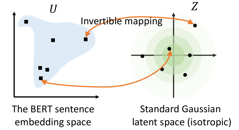
Figure 1: An illustration of our proposed flow-based calibration over the original sentence embedding space of BERT.

3.1 Motivation

A standard Gaussian latent space may have favorable properties which can help with our problem.

Connection to Observation 1

First, standard Gaussian satisfies isotropy. The probabilistic density in standard Gaussian distribution does not vary in terms of angle. If the $\ell_{2}$ norm of samples from standard Gaussian are normalized to 1, these samples can be regarded as uniformly distributed over a unit sphere.

We can also understand the isotropy from a singular spectrum perspective. As discussed above, the anisotropy of the embedding space stems from the imbalance of word frequency. In the literature of traditional word embeddings, Mu et al. (2017) discovers that the dominating singular vectors can be highly correlated to word frequency, which misleads the embedding space. By fitting a mapping to an isotropic distribution, the singular spectrum of the embedding space can be flattened. In this way, the word frequency-related singular directions, which are the dominating ones, can be suppressed.

Connection to Observation 2

Second, the probabilistic density of Gaussian is well defined over the entire real space. This means there are no “hole” areas, which are poorly defined in terms of probability. The helpfulness of Gaussian prior for mitigating the “hole” problem has been widely observed in existing literature of deep latent variable models (Rezende and Viola, 2018; Li et al., 2019; Ghosh et al., 2020).

3.2 Flow-based Generative Model

We instantiate the invertible mapping with flows. A flow-based generative model Kobyzev et al. (2019) establishes an invertible transformation from the latent space $\mathcal{Z}$ to the observed space $\mathcal{U}$. The generative story of the model is defined as

$${\mathbf{z}}\sim p_{\mathcal{Z}}({\mathbf{z}}),{\mathbf{u}}=f_{\phi}({\mathbf{z}})\vspace{-5pt}$$

where ${\mathbf{z}}\sim p_{\mathcal{Z}}(\mathbf{{\mathbf{z}}})$ the prior distribution, and $f:\mathcal{Z}\rightarrow\mathcal{U}$ is an invertible transformation. With the change-of-variables theorem, the probabilistic density function (PDF) of the observable $x$ is given as,

$$p_{\mathcal{U}}({\mathbf{u}})=p_{\mathcal{Z}}(f_{\phi}^{-1}({\mathbf{u}}))~{}\lvert\textrm{det}\frac{\partial f_{\phi}^{-1}({\mathbf{u}})}{\partial{\mathbf{u}}}\rvert$$

In our method, we learn a flow-based generative model by maximizing the likelihood of generating BERT sentence embeddings from a standard Gaussian latent latent variable. In other words, the base distribution $p_{\mathcal{Z}}$ is a standard Gaussian and we consider the extracted BERT sentence embeddings as the observed space $\mathcal{U}$. We maximize the likelihood of $\mathcal{U}$’s marginal via Equation 3.2 in a fully unsupervised way.

$$\vspace{-10pt}\textrm{max}_{\phi}~{} \mathbb{E}_{{\mathbf{u}}=\textrm{BERT(sentence)},\textrm{sentence}\sim\mathcal{D}}$$

$$\log p_{\mathcal{Z}}(f_{\phi}^{-1}({\mathbf{u}}))+\log~{}\lvert\textrm{det}\frac{\partial f_{\phi}^{-1}({\mathbf{u}})}{\partial{\mathbf{u}}}\rvert,\vspace{-5pt}$$ (4)

Here $\mathcal{D}$ denotes the dataset, in other words, the collection of sentences. Note that during training, only the flow parameters are optimized while the BERT parameters remain unchanged. Eventually, we learn an invertible mapping function $f_{\phi}^{-1}$ which can transform each BERT sentence embedding ${\mathbf{u}}$ into a latent Gaussian representation ${\mathbf{z}}$ without loss of information.

The invertible mapping $f_{\phi}$ is parameterized as a neural network, and the architectures are usually carefully designed to guarantee the invertibility Dinh et al. (2015). Moreover, its determinant $\lvert\textrm{det}\frac{\partial f_{\phi}^{-1}({\mathbf{u}})}{\partial{\mathbf{u}}}\rvert$ should also be easy to compute so as to make the maximum likelihood training tractable. In our experiments, we follows the design of Glow Kingma and Dhariwal (2018). The Glow model is composed of a stack of multiple invertible transformations, namely actnorm, invertible $1\times 1$ convolution, and affine coupling layer. We simplify the model by replacing affine coupling with additive coupling Dinh et al. (2015) to reduce model complexity, and replacing the invertible $1\times 1$ convolution with random permutation to avoid numerical errors. For the mathematical formula of the flow model with additive coupling, please refer to Appendix A.

4 Experiments

Dataset	STS-B	SICK-R	STS-12	STS-13	STS-14	STS-15	STS-16
Published in Reimers and Gurevych (2019)
Avg. GloVe embeddings	58.02	53.76	55.14	70.66	59.73	68.25	63.66
Avg. BERT embeddings	46.35	58.40	38.78	57.98	57.98	63.15	61.06
BERT CLS-vector	16.50	42.63	20.16	30.01	20.09	36.88	38.03
Our Implementation
BERT${}_{\text{base}}$	47.29	58.21	49.07	55.92	54.75	62.75	65.19
BERT${}_{\text{base}}$-last2avg	59.04	63.75	57.84	61.95	62.48	70.95	69.81
BERT${}_{\text{base}}$-flow (NLI∗)	58.56 ($\leavevmode\color[rgb]{1,0,0}\downarrow$)	65.44 ($\leavevmode\color[rgb]{0,1,0}\uparrow$)	59.54 ($\leavevmode\color[rgb]{0,1,0}\uparrow$)	64.69 ($\leavevmode\color[rgb]{0,1,0}\uparrow$)	64.66 ($\leavevmode\color[rgb]{0,1,0}\uparrow$)	72.92 ($\leavevmode\color[rgb]{0,1,0}\uparrow$)	71.84 ($\leavevmode\color[rgb]{0,1,0}\uparrow$)
BERT${}_{\text{base}}$-flow (target)	70.72 ($\leavevmode\color[rgb]{0,1,0}\uparrow$)	63.11($\leavevmode\color[rgb]{1,0,0}\downarrow$)	63.48 ($\leavevmode\color[rgb]{0,1,0}\uparrow$)	72.14 ($\leavevmode\color[rgb]{0,1,0}\uparrow$)	68.42 ($\leavevmode\color[rgb]{0,1,0}\uparrow$)	73.77 ($\leavevmode\color[rgb]{0,1,0}\uparrow$)	75.37 ($\leavevmode\color[rgb]{0,1,0}\uparrow$)
BERT${}_{\text{large}}$	46.99	53.74	46.89	53.32	49.27	56.54	61.63
BERT${}_{\text{large}}$-last2avg	59.56	60.22	57.68	61.37	61.02	68.04	70.32
BERT${}_{\text{large}}$-flow (NLI∗)	68.09 ($\leavevmode\color[rgb]{0,1,0}\uparrow$)	64.62 ($\leavevmode\color[rgb]{0,1,0}\uparrow$)	61.72 ($\leavevmode\color[rgb]{0,1,0}\uparrow$)	66.05 ($\leavevmode\color[rgb]{0,1,0}\uparrow$)	66.34 ($\leavevmode\color[rgb]{0,1,0}\uparrow$)	74.87 ($\leavevmode\color[rgb]{0,1,0}\uparrow$)	74.47 ($\leavevmode\color[rgb]{0,1,0}\uparrow$)
BERT${}_{\text{large}}$-flow (target)	72.26 ($\leavevmode\color[rgb]{0,1,0}\uparrow$)	62.50 ($\leavevmode\color[rgb]{0,1,0}\uparrow$)	65.20 ($\leavevmode\color[rgb]{0,1,0}\uparrow$)	73.39 ($\leavevmode\color[rgb]{0,1,0}\uparrow$)	69.42 ($\leavevmode\color[rgb]{0,1,0}\uparrow$)	74.92 ($\leavevmode\color[rgb]{0,1,0}\uparrow$)	77.63 ($\leavevmode\color[rgb]{0,1,0}\uparrow$)

Table 2: Experimental results on semantic textual similarity without using NLI supervision. We report the Spearman’s rank correlation between the cosine similarity of sentence embeddings and the gold labels on multiple datasets. Numbers are reported as $\rho\times 100$. $\leavevmode\color[rgb]{0,1,0}\uparrow$ denotes outperformance over its BERT baseline and $\leavevmode\color[rgb]{1,0,0}\downarrow$ denotes underperformance. Our proposed BERT-flow method achieves the best scores. Note that our BERT-flow use -last2avg as default setting. $*$: Use NLI corpus for the unsupervised training of flow; supervision labels of NLI are NOT visible.

To verify our hypotheses and demonstrate the effectiveness of our proposed method, in this section we present our experimental results for various tasks related to semantic textual similarity under multiple configurations. For the implementation details of our siamese BERT models and flow-based models, please refer to Appendix B.

4.1 Semantic Textual Similarity

Datasets.

We evaluate our approach extensively on the semantic textual similarity (STS) tasks. We report results on 7 datasets, namely the STS benchmark (STS-B) (Cer et al., 2017) the SICK-Relatedness (SICK-R) dataset (Marelli et al., 2014) and the STS tasks 2012 - 2016 (Agirre et al., 2012, 2013, 2014, 2015, 2016). We obtain all these datasets via the SentEval toolkit (Conneau and Kiela, 2018). These datasets provide a fine-grained gold standard semantic similarity between 0 and 5 for each sentence pair.

Evaluation Procedure.

Following the procedure in previous work like Sentence-BERT Reimers and Gurevych (2019) for the STS task, the prediction of similarity consists of two steps: (1) first, we obtain sentence embeddings for each sentence with a sentence encoder, and (2) then, we compute the cosine similarity between the two embeddings of the input sentence pair as our model-predicted similarity. The reported numbers are the Spearman’s correlation coefficients between the predicted similarity and gold standard similarity scores, which is the same way as in (Reimers and Gurevych, 2019).

Experimental Details.

We consider both BERT${}_{\text{base}}$ and BERT${}_{\text{large}}$ in our experiments. Specifically, we use an average pooling over BERT context embeddings in the last one or two layers as the sentence embedding which is found to outperform the [CLS] vector. Interestingly, our preliminary exploration shows that averaging the last two layers of BERT (denoted by -last2avg) consistently produce better results compared to only averaging the last one layer. Therefore, we choose -last2avg as our default configuration when assessing our own approach.

For the proposed method, the flow-based objective (Equation 3.2) is maximized only to update the invertible mapping while the BERT parameters remains unchanged. Our flow models are by default learned over the full target dataset (train + validation + test). We denote this configuration as flow (target). Note that although we use the sentences of the entire target dataset, learning flow does not use any provided labels for training, thus it is a purely unsupervised calibration over the BERT sentence embedding space.

We also test our flow-based model learned on a concatenation of SNLI (Bowman et al., 2015) and MNLI (Williams et al., 2018) for comparison (flow (NLI)). The concatenated NLI datasets comprise of tremendously more sentence pairs (SNLI 570K + MNLI 433K). Note that “flow (NLI)” does not require any supervision label. When fitting flow on NLI corpora, we only use the raw sentences instead of the entailment labels. An intuition behind the flow (NLI) setting is that, compared to Wikipedia sentences (on which BERT is pretrained), the raw sentences of both NLI and STS are simpler and shorter. This means the NLI-STS discrepancy could be relatively smaller than the Wikipedia-STS discrepancy.

We run the experiments on two settings: (1) when external labeled data is unavailable. This is the natural setting where we learn flow parameters with the unsupervised objective (Equation 3.2), meanwhile BERT parameters are unchanged. (2) we first fine-tune BERT on the SNLI+MNLI textual entailment classification task in a siamese fashion (Reimers and Gurevych, 2019). For BERT-flow, we further learn the flow parameters. This setting is to compare with the state-of-the-art results which utilize NLI supervision (Reimers and Gurevych, 2019). We denote the two different models as BERT-NLI and BERT-NLI-flow respectively.

Dataset	STS-B	SICK-R	STS-12	STS-13	STS-14	STS-15	STS-16
Published in Reimers and Gurevych (2019)
InferSent - Glove	68.03	65.65	52.86	66.75	62.15	72.77	66.86
USE	74.92	76.69	64.49	67.80	64.61	76.83	73.18
SBERT${}_{\text{base}}$-NLI	77.03	72.91	70.97	76.53	73.19	79.09	74.30
SBERT${}_{\text{large}}$-NLI	79.23	73.75	72.27	78.46	74.90	80.99	76.25
SRoBERTa${}_{\text{base}}$-NLI	77.77	74.46	71.54	72.49	70.80	78.74	73.69
SRoBERTa${}_{\text{large}}$-NLI	79.10	74.29	74.53	77.00	73.18	81.85	76.82
Our Implementation
BERT${}_{\text{base}}$-NLI	77.08	72.62	66.23	70.22	72.15	77.35	73.91
BERT${}_{\text{base}}$-NLI-last2avg	78.03	74.07	68.37	72.44	73.98	79.15	75.39
BERT${}_{\text{base}}$-NLI-flow (NLI∗)	79.10 ($\leavevmode\color[rgb]{0,1,0}\uparrow$)	78.03 ($\leavevmode\color[rgb]{0,1,0}\uparrow$)	67.75 ($\leavevmode\color[rgb]{1,0,0}\downarrow$)	76.73 ($\leavevmode\color[rgb]{0,1,0}\uparrow$)	75.53 ($\leavevmode\color[rgb]{0,1,0}\uparrow$)	80.63 ($\leavevmode\color[rgb]{0,1,0}\uparrow$)	77.58 ($\leavevmode\color[rgb]{0,1,0}\uparrow$)
BERT${}_{\text{base}}$-NLI-flow (target)	81.03 ($\leavevmode\color[rgb]{0,1,0}\uparrow$)	74.97 ($\leavevmode\color[rgb]{0,1,0}\uparrow$)	68.95 ($\leavevmode\color[rgb]{0,1,0}\uparrow$)	78.48 ($\leavevmode\color[rgb]{0,1,0}\uparrow$)	77.62 ($\leavevmode\color[rgb]{0,1,0}\uparrow$)	81.95 ($\leavevmode\color[rgb]{0,1,0}\uparrow$)	78.94 ($\leavevmode\color[rgb]{0,1,0}\uparrow$)
BERT${}_{\text{large}}$-NLI	77.80	73.44	66.87	73.91	74.04	79.14	75.35
BERT${}_{\text{large}}$-NLI-last2avg	78.45	74.93	68.69	75.63	75.55	80.35	76.81
BERT${}_{\text{large}}$-NLI-flow (NLI∗)	79.89 ($\leavevmode\color[rgb]{0,1,0}\uparrow$)	77.73 ($\leavevmode\color[rgb]{0,1,0}\uparrow$)	69.61 ($\leavevmode\color[rgb]{0,1,0}\uparrow$)	79.45 ($\leavevmode\color[rgb]{0,1,0}\uparrow$)	77.56 ($\leavevmode\color[rgb]{0,1,0}\uparrow$)	82.48 ($\leavevmode\color[rgb]{0,1,0}\uparrow$)	79.36 ($\leavevmode\color[rgb]{0,1,0}\uparrow$)
BERT${}_{\text{large}}$-NLI-flow (target)	81.18 ($\leavevmode\color[rgb]{0,1,0}\uparrow$)	74.52 ($\leavevmode\color[rgb]{1,0,0}\downarrow$)	70.19 ($\leavevmode\color[rgb]{0,1,0}\uparrow$)	80.27 ($\leavevmode\color[rgb]{0,1,0}\uparrow$)	78.85 ($\leavevmode\color[rgb]{0,1,0}\uparrow$)	82.97 ($\leavevmode\color[rgb]{0,1,0}\uparrow$)	80.57 ($\leavevmode\color[rgb]{0,1,0}\uparrow$)

Table 3: Experimental results on semantic textual similarity with NLI supervision. Note that our flows are still learned in a unsupervised way. InferSent (Conneau et al., 2017) is a siamese LSTM train on NLI, Universal Sentence Encoder (USE) (Cer et al., 2018) replace the LSTM with a Transformer and SBERT Reimers and Gurevych (2019) further use BERT. We report the Spearman’s rank correlation between the cosine similarity of sentence embeddings and the gold labels on multiple datasets. Numbers are reported as $\rho\times 100$. $\leavevmode\color[rgb]{0,1,0}\uparrow$ denotes outperformance over its BERT baseline and $\leavevmode\color[rgb]{1,0,0}\downarrow$ denotes underperformance. Our proposed BERT-flow (i.e., the “BERT-NLI-flow” in this table) method achieves the best scores. Note that our BERT-flow use -last2avg as default setting. $*$: Use NLI corpus for the unsupervised training of flow; supervision labels of NLI are NOT visible.

Results w/o NLI Supervision.

As shown in Table 2, the original BERT sentence embeddings (with both BERT${}_{\text{base}}$ and BERT${}_{\text{large}}$) fail to outperform the averaged GloVe embeddings. And averaging the last-two layers of the BERT model can consistently improve the results. For BERT${}_{\text{base}}$ and BERT${}_{\text{large}}$, our proposed flow-based method (BERT-flow (target)) can further boost the performance by 5.88 and 8.16 points on average respectively. For most of the datasets, learning flows on the target datasets leads to larger performance improvement than on NLI. The only exception is SICK-R where training flows on NLI is better. We think this is because SICK-R is collected for both entailment and relatedness. Since SNLI and MNLI are also collected for textual entailment evaluation, the distribution discrepancy between SICK-R and NLI may be relatively small. Also due to the much larger size of the NLI datasets, it is not surprising that learning flows on NLI results in stronger performance.

Results w/ NLI Supervision.

Table 3 shows the results with NLI supervisions. Similar to the fully unsupervised results before, our isotropic embedding space from invertible transformation is able to consistently improve the SBERT baselines in most cases, and outperforms the state-of-the-art SBERT/SRoBERTa results by a large margin. Robustness analysis with respect to random seeds are provided in Appendix C.

4.2 Unsupervised Question-Answer Entailment

In addition to the semantic textual similarity tasks, we examine the effectiveness of our method on unsupervised question-answer entailment. We use Question Natural Language Inference (QNLI, Wang et al. (2019)), a dataset comprising 110K question-answer pairs (with 5K+ for testing). QNLI extracts the questions as well as their corresponding context sentences from SQUAD (Rajpurkar et al., 2016), and annotates each pair as either entailment or no entailment. In this paper, we further adapt QNLI as an unsupervised task. The similarity between a question and an answer can be predicted by computing the cosine similarity of their sentence embeddings. Then we regard entailment as 1 and no entailment as 0, and evaluate the performance of the methods with AUC.

As shown in Table 4, our method consistently improves the AUC on the validation set of QNLI. Also, learning flow on the target dataset can produce superior results compared to learning flows on NLI.

Method	AUC
BERT${}_{\text{base}}$-NLI-last2avg	70.30
BERT${}_{\text{base}}$-NLI-flow (NLI∗)	72.52 ($\leavevmode\color[rgb]{0,1,0}\uparrow$)
BERT${}_{\text{base}}$-NLI-flow (target)	76.17 ($\leavevmode\color[rgb]{0,1,0}\uparrow$)
BERT${}_{\text{large}}$-NLI-last2avg	70.41
BERT${}_{\text{large}}$-NLI-flow (NLI∗)	74.19 ($\leavevmode\color[rgb]{0,1,0}\uparrow$)
BERT${}_{\text{large}}$-NLI-flow (target)	77.09 ($\leavevmode\color[rgb]{0,1,0}\uparrow$)

Table 4: AUC on QNLI evaluated on the validation set. $*$: Use NLI corpus for the unsupervised training of flow; supervision labels of NLI are NOT visible.

4.3 Comparison with Other Embedding Calibration Baselines

Method	Correlation
BERT${}_{\text{base}}$	47.29
+ SN	55.46
+ NATSV ($k=1$)	51.79
+ NATSV ($k=10$)	60.40
+ SN + NATSV ($k=1$)	56.02
+ SN + NATSV ($k=6$)	63.51
BERT${}_{\text{base}}$-flow (target)	65.62

Table 5: Comparing flow-based method with baselines on STS-B. $k$ is selected among $1\sim 20$ on the validation set. We report the Spearman’s rank correlation ($\times 100$).

In the literature of traditional word embeddings, Arora et al. (2017) and Mu et al. (2017) also discover the anisotropy phenomenon of the embedding space, and they provide several methods to encourage isotropy:

Standard Normalization (SN).

In this idea, we conduct a simple post-processing over the embeddings by computing the mean $\bm{\mathbf{\mu}}$ and standard deviation $\bm{\mathbf{\sigma}}$ of the sentence embeddings ${\mathbf{u}}$’s, and normalizing the embeddings by $\frac{{\mathbf{u}}-\bm{\mathbf{\mu}}}{\bm{\mathbf{\sigma}}}$.

Nulling Away Top-$k$ Singular Vectors (NATSV).

Mu et al. (2017) find out that sentence embeddings computed by averaging traditional word embeddings tend to have a fast-decaying singular spectrum. They claim that, by nulling away the top-$k$ singular vectors, the anisotropy of the embeddings can be circumvented and better semantic similarity performance can be achieved.

We compare with these embedding calibration methods on STS-B dataset and the results are shown in Table 5. Standard normalization (SN) helps improve the performance but it falls behind nulling away top-$k$ singular vectors (NATSV). This means standard normalization cannot fundamentally eliminate the anisotropy. By combining the two methods, and carefully tuning $k$ over the validation set, further improvements can be achieved. Nevertheless, our method still produces much better results. We argue that NATSV can help eliminate anisotropy but it may also discard some useful information contained in the nulled vectors. On the contrary, our method directly learns an invertible mapping to isotropic latent space without discarding any information.

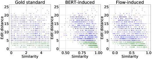
Figure 2: A scatterplot of sentence pairs, where the horizontal axis represents similarity (either gold standard semantic similarity or embedding-induced similarity), the vertical axis represents edit distance. The sentence pairs with edit distance $\leq 4$ are highlighted with green, meanwhile the rest of the pairs are colored with blue. We can observed that lexically similar sentence pairs tends to be predicted to be similar by BERT embeddings, especially for the green pairs. Such correlation is less evident for gold standard labels or flow-induced embeddings.

4.4 Dicussion: Semantic Similarity Versus Lexical Similarity

In addition to semantic similarity, we further study lexical similarity induced by different sentence embeddings. Specifically, we use edit distance as the metric for lexical similarity between a pair of sentences, and focus on the correlations between the sentence similarity and edit distance. Concretely, we compute the cosine similarity in terms of BERT sentence embeddings as well as edit distance for each sentence pair. Within a dataset consisting of many sentence pairs, we compute the Spearman’s correlation coefficient $\rho$ between the similarities and the edit distances, as well as between similarities from different models. We perform experiment on the STS-B dataset and include the human annotated gold similarity into this analysis.

BERT-Induced Similarity Excessively Correlates with Lexical Similarity.

Similarity	Edit distance	Gold similarity
Gold similarity	-24.61	100.00
BERT-induce similarity	-50.49	59.30
Flow-induce similarity	-28.01	74.09

Table 6: Spearman’s correlation $\rho$ between various sentence similarities on the validation set of STS-B. We can observe that BERT-induced similarity is highly correlated to edit distance, while the correlation with edit distance is less evident for gold standard or flow-induced similarity.

Table 6 shows that the correlation between BERT-induced similarity and edit distance is very strong ($\rho=-50.49$), considering that gold standard labels maintain a much smaller correlation with edit distance ($\rho=-24.61$). This phenomenon can also be observed in Figure 2. Especially, for sentence pairs with edit distance $\leq 4$ (highlighted with green), BERT-induced similarity is extremely correlated to edit distance. However, it is not evident that gold standard semantic similarity correlates with edit distance. In other words, it is often the case where the semantics of a sentence can be dramatically changed by modifying a single word. For example, the sentences “I like this restaurant” and “I dislike this restaurant” only differ by one word, but convey opposite semantic meaning. BERT embeddings may fail in such cases. Therefore, we argue that the lexical proximity of BERT sentence embeddings is excessive, and can spoil their induced semantic similarity.

Flow-Induced Similarity Exhibits Lower Correlation with Lexical Similarity.

By transforming the original BERT sentence embeddings into the learned isotropic latent space with flow, the embedding-induced similarity not only aligned better with the gold semantic semantic similarity, but also shows a lower correlation with lexical similarity, as presented in the last row of Table 6. The phenomenon is especially evident for the examples with edit distance $\leq 4$ (highlighted with green in Figure 2). This demonstrates that our proposed flow-based method can effectively suppress the excessive influence of lexical similarity over the embedding space.

5 Conclusion and Future Work

In this paper, we investigate the deficiency of the BERT sentence embeddings on semantic textual similarity, and propose a flow-based calibration which can effectively improve the performance. In the future, we are looking forward to diving in representation learning with flow-based generative models from a broader perspective.

Appendix A Mathematical Formula of the Invertible Mapping

Generally, flow-based model is a stacked sequence of many invertible transformation layers: $f=f_{1}\circ f_{2}\circ\ldots\circ f_{K}$. Specifically, in our approach, each transformation $f_{i}:x\rightarrow y$ is an additive coupling layer, which can be mathematically formulated as follows.

$$y_{1:d} =x_{1:d}$$ (5)

$$y_{d+1:D} =x_{d+1:D}+g_{\psi}(x_{1:d}).$$ (6)

Here $g_{\psi}$ can be parameterized with a deep neural network for the sake of expressiveness.

Its inverse function $f_{i}^{-1}:y\rightarrow x$ can be explicitly written as:

$$x_{1:d} =y_{1:d}$$ (7)

$$x_{d+1:D} =y_{d+1:D}-g_{\psi}(y_{1:d}).$$ (8)

Appendix B Implementation Details

Throughout our experiment, we adopt the official Tensorflow code of BERT  as our codebase. Note that we clip the maximum sequence length to 64 to reduce the costing of GPU memory. For the NLI finetuning of siamese BERT, we folllow the settings in (Reimers and Gurevych, 2019) (epochs = 1, learning rate = $2e-5$, and batch size = 16). Our results may vary from their published one. The authors mentioned in https://github.com/UKPLab/sentence-transformers/issues/50 that this is a common phenonmenon and might be related the random seed. Note that their implementation relies on the Transformers repository of Huggingface. This may also lead to discrepancy between the specific numbers.

Our implementation of flows is adapted from both the official repository of GLOW as well as the implementation fo the Tensor2tensor library. The hyperparameters of our flow models are given in Table 7. On the target datasets, we learn the flow parameters for 1 epoch with learning rate $1e-3$. On NLI datasets, we learn the flow parameters for 0.15 epoch with learning rate $2e-5$. The optimizer that we use is Adam.

In our preliminary experiments on STS-B, we tune the hyperparameters on the dev set of STS-B. Empirically, the performance does not vary much with regard to the architectural hyperparameters compared to the learning schedule. Afterwards, we do not tune the hyperparameters any more when working on the other datasets. Empirically, we find the hyperparameters of flow are not sensitive across the datasets.

Coupling architecture in	3-layer CNN with residual connection
Coupling width	32
#levels	2
Depth	3

Table 7: Flow hyperparameters.

Appendix C Results with Different Random Seeds

We perform 5 runs with different random seeds in the NLI-supervised setting on STS-B. Results with standard deviation and median are demonstrated in Table 8. Although the variance of NLI finetuning is not negligible, our proposed flow-based method consistently leads to improvement.

Method	Spearman’s $\rho$
BERT-NLI-large	77.26 $\pm$ 1.76 (median: 78.19)
BERT-NLI-large-last2avg	78.07 $\pm$ 1.50 (median: 78.68)
BERT-NLI-large-last2avg + flow-target	81.10 $\pm$ 0.55 (median: 81.35)

Table 8: Results with different random seeds.

References

- Agirre et al. (2015) Eneko Agirre, Carmen Banea, Claire Cardie, Daniel Cer, Mona Diab, Aitor Gonzalez-Agirre, Weiwei Guo, Inigo Lopez-Gazpio, Montse Maritxalar, Rada Mihalcea, et al. 2015. SemEval-2015 task 2: Semantic textual similarity, english, spanish and pilot on interpretability. In Proceedings of SemEval.
- Agirre et al. (2014) Eneko Agirre, Carmen Banea, Claire Cardie, Daniel Cer, Mona Diab, Aitor Gonzalez-Agirre, Weiwei Guo, Rada Mihalcea, German Rigau, and Janyce Wiebe. 2014. SemEval-2014 task 10: Multilingual semantic textual similarity. In Proceedings of SemEval.
- Agirre et al. (2016) Eneko Agirre, Carmen Banea, Daniel Cer, Mona Diab, Aitor Gonzalez Agirre, Rada Mihalcea, German Rigau Claramunt, and Janyce Wiebe. 2016. SemEval-2016 task 1: Semantic textual similarity, monolingual and cross-lingual evaluation. In Proceedings of SemEval.
- Agirre et al. (2012) Eneko Agirre, Daniel Cer, Mona Diab, and Aitor Gonzalez-Agirre. 2012. SemEval-2012 task 6: A pilot on semantic textual similarity. In Proceedings of SemEval.
- Agirre et al. (2013) Eneko Agirre, Daniel Cer, Mona Diab, Aitor Gonzalez-Agirre, and Weiwei Guo. 2013. * SEM 2013 shared task: Semantic textual similarity. In Proceedings of SemEval.
- Arora et al. (2017) Sanjeev Arora, Yingyu Liang, and Tengyu Ma. 2017. A simple but tough-to-beat baseline for sentence embeddings. In Proceedings of ICLR.
- Bowman et al. (2015) Samuel R Bowman, Gabor Angeli, Christopher Potts, and Christopher D Manning. 2015. A large annotated corpus for learning natural language inference. In Proceedings of EMNLP.
- Cer et al. (2017) Daniel Cer, Mona Diab, Eneko Agirre, Inigo Lopez-Gazpio, and Lucia Specia. 2017. SemEval-2017 task 1: Semantic textual similarity-multilingual and cross-lingual focused evaluation. arXiv preprint arXiv:1708.00055.
- Cer et al. (2018) Daniel Cer, Yinfei Yang, Sheng-yi Kong, Nan Hua, Nicole Limtiaco, Rhomni St John, Noah Constant, Mario Guajardo-Cespedes, Steve Yuan, Chris Tar, et al. 2018. Universal sentence encoder. arXiv preprint arXiv:1803.11175.
- Conneau and Kiela (2018) Alexis Conneau and Douwe Kiela. 2018. SentEval: An evaluation toolkit for universal sentence representations. In Proceedings of LREC.
- Conneau et al. (2017) Alexis Conneau, Douwe Kiela, Holger Schwenk, Loïc Barrault, and Antoine Bordes. 2017. Supervised learning of universal sentence representations from natural language inference data. In Proceedings of EMNLP.
- Devlin et al. (2019) Jacob Devlin, Ming-Wei Chang, Kenton Lee, and Kristina Toutanova. 2019. BERT: Pre-training of deep bidirectional transformers for language understanding. In Proceedings of NAACL.
- Dinh et al. (2015) Laurent Dinh, David Krueger, and Yoshua Bengio. 2015. NICE: Non-linear independent components estimation. In Proceedings of ICLR.
- Ethayarajh (2019) Kawin Ethayarajh. 2019. How contextual are contextualized word representations? comparing the geometry of bert, elmo, and gpt-2 embeddings. In Proceedings of EMNLP-IJCNLP.
- Ethayarajh et al. (2019) Kawin Ethayarajh, David Duvenaud, and Graeme Hirst. 2019. Towards understanding linear word analogies. In Proceedings of ACL.
- Gao et al. (2019) Jun Gao, Di He, Xu Tan, Tao Qin, Liwei Wang, and Tie-Yan Liu. 2019. Representation degeneration problem in training natural language generation models. In Proceedings of ICLR.
- Ghosh et al. (2020) Partha Ghosh, Mehdi SM Sajjadi, Antonio Vergari, Michael Black, and Bernhard Scholkopf. 2020. From variational to deterministic autoencoders. In Proceedings of ICLR.
- Kingma and Dhariwal (2018) Durk P Kingma and Prafulla Dhariwal. 2018. Glow: Generative flow with invertible 1x1 convolutions. In Proceedings of NeurIPS.
- Kobyzev et al. (2019) Ivan Kobyzev, Simon Prince, and Marcus A Brubaker. 2019. Normalizing flows: Introduction and ideas. arXiv preprint arXiv:1908.09257.
- Levy and Goldberg (2014) Omer Levy and Yoav Goldberg. 2014. Neural word embedding as implicit matrix factorization. In Proceedings of NeurIPS.
- Li et al. (2019) Bohan Li, Junxian He, Graham Neubig, Taylor Berg-Kirkpatrick, and Yiming Yang. 2019. A surprisingly effective fix for deep latent variable modeling of text. In Proceedings of EMNLP-IJCNLP.
- Liu et al. (2019) Yinhan Liu, Myle Ott, Naman Goyal, Jingfei Du, Mandar Joshi, Danqi Chen, Omer Levy, Mike Lewis, Luke Zettlemoyer, and Veselin Stoyanov. 2019. RoBERTa: A robustly optimized BERT pretraining approach. arXiv preprint arXiv:1907.11692.
- Marelli et al. (2014) Marco Marelli, Stefano Menini, Marco Baroni, Luisa Bentivogli, Raffaella Bernardi, Roberto Zamparelli, et al. 2014. A SICK cure for the evaluation of compositional distributional semantic models. In Proceedings of LREC.
- Mu et al. (2017) Jiaqi Mu, Suma Bhat, and Pramod Viswanath. 2017. All-but-the-top: Simple and effective postprocessing for word representations. In Proceedings of ICLR.
- Pennington et al. (2014) Jeffrey Pennington, Richard Socher, and Christopher D Manning. 2014. GloVe: Global vectors for word representation. In Proceedings of EMNLP.
- Radford et al. (2019) Alec Radford, Jeffrey Wu, Rewon Child, David Luan, Dario Amodei, and Ilya Sutskever. 2019. Language models are unsupervised multitask learners. OpenAI Blog, 1(8).
- Rajpurkar et al. (2016) Pranav Rajpurkar, Jian Zhang, Konstantin Lopyrev, and Percy Liang. 2016. SQuAD: 100,000+ questions for machine comprehension of text. In Proceedings of EMNLP.