An understanding of the physical solutions and the blow-up phenomenon for Nonlinear Noisy Leaky Integrate and Fire neuronal models

Abstract

The Nonlinear Noisy Leaky Integrate and Fire neuronal models are mathematical models that describe the activity of neural networks. These models have been studied at a microscopic level, using Stochastic Differential Equations, and at a mesoscopic/macroscopic level, through the mean field limits using Fokker-Planck type equations. The aim of this paper is to improve their understanding, using a numerical study of their particle systems. We analyse in depth the behaviour of the classical and physical solutions of the Stochastic Differential Equations and, we compare it with what is already known about the Fokker-Planck equation. This allows us to better understand what happens in the neural network when an explosion occurs in finite time. After firing all neurons at the same time, if the system is weakly connected, the neural network converges towards its unique steady state. Otherwise, its behaviour is more complex, because it can tend towards a stationary state or a “plateau” distribution.

1 Introduction

Nonlinear Noisy Leaky Integrate and Fire neuronal (NNLIF) models are one of the simplest models used to describe the behaviour of a neuronal network [23, 37, 28, 3, 2, 4]. In recent years, NNLIF models have been studied from a mathematical point of view; at the microscopic level, using Stochastic Differential Equations (SDE) [17, 16, 24], and at a mesoscopic/macroscopic level, through the mean field limits using Fokker-Planck type equations (FPE) [5, 12, 7, 9, 10, 8, 22, 36]. The considerable amount of publications and unanswered questions on these models reveal their high mathematical complexity, despite their simplicity.

The aim of this paper is to advance the understanding of the NNLIF models. We analyse in depth the behaviour of the classical and physical solutions of the Stochastic Differential Equations and we compare it with what is already known about the Fokker-Planck equation, using a numerical study of their particle systems. This allows us to better understand what happens in the neural network when an explosion occurs in finite time, which is one of the most important open problems about this kind of models.

1.1 Stochastic Differential Equation and Fokker-Planck Equation

Let us consider a large set of $\mathcal{N}$ identical neurons which are connected to each other in a network and described by the Nonlinear Noisy Leaky Integrate and Fire (NNLIF) model. This model represents the network activity in relation to the membrane potential, which is the potential difference on both sides of the neuronal membrane. The membrane potential $V_{i}(t)$ of a single neuron $i$ is given by [4, 3, 15, 35]:

$$C_{m}\dot{V}_{i}(t)=-g_{L}(V_{i}(t)-V_{L})+I_{i}(t),\quad i=1,\ldots,\mathcal{N},$$ (1)

where $C_{m}$ is the capacitance of the membrane, $g_{L}$ is the leak conductance, $V_{L}$ is the resting potential and $I_{i}(t)$ are the synaptic currents. These currents are produced by the local and external synapses, i.e. they are the sum of spikes received from $C$ neurons (inside and outside the neuron network):

$$I_{i}(t)=\sum_{j}\sum_{k}J_{ij}\delta(t-t_{ik}^{j}-\delta).$$ (2)

The Dirac delta $\delta(t-t_{ik}^{j}-\delta)$ models the input contribution of each spike; $t_{ik}^{j}$ is the time when the $k$-th spike of the $j$-th neuron took place, $J_{ij}$ is the synaptic strength (positive value for excitatory neurons and negative value for inhibitory ones), and $\delta$ in the argument is the synaptic delay.

A neuron spikes when its membrane voltage reaches the firing threshold value $V_{F}$. Then, the neuron discharges itself by sending a spike perturbation over the network, and its membrane potential is set to the reset value $V_{R}$. The relation between the three values $V_{L}$, $V_{F}$ and $V_{R}$ is the following: $V_{L}<V_{R}<V_{F}$.

We consider networks in which pair correlations can be neglected, as a consequence of the network sparse random connectivity, i.e., $C/\mathcal{N}\ll 1$. We also consider each input as a small contribution compared to the firing threshold ($|J_{ij}|\ll V_{F}$). Under these conditions (see [4] for more details), if we assume every neuron in the network to spikes according to Poisson processes with a common instantaneous probability of emitting a spike per unit time $\nu$ (firing rate), we can describe the synaptic current of a neuron as

$$I_{i}(t)\simeq\mu_{c}(t)+\sigma_{c}\eta_{i}(t)$$ (3)

where $\mu_{c}=b\nu(t-\delta)$ represents the average value of the current (taking into account the excitatory and inhibitory neurons in the network), $\sigma^{2}_{c}=\alpha\nu(t-\delta)$ its variance, and $\eta_{i}(t)$ are independent Gaussian white noises. The constant $\alpha$ depends on the number and the strength of excitatory and inhibitory neurons. The parameter $b$ will be called the connectivity parameter and its value shows how excited or inhibited the network is. If $b>0$ the network is average-excitatory; a high value of $b$ means that neurons are highly connected, on the other hand $b<0$ describes a network which is average-inhibitory. The limiting case $b=0$ means that neurons are not connected with each other and the system becomes linear.

As we mentioned above, the equation (1) is completed with the following boundary condition: $V_{i}(t_{s}^{-})=V_{F}$ and $V_{i}(t_{s}^{+})=V_{R}$, with $t_{s}$ the firing time of neuron $i$.

Without loss of generality, we will take $C_{m}=g_{L}=1$. We rewrite $\nu(t)=\nu_{ext}+N(t)$, splitting according to external, $\nu_{ext}$, and internal, $N(t)$, activity; where $\nu_{ext}$ is a constant and $N(t)$ is the firing rate of the network, and $\sigma_{c}=\sqrt{2a(N)}$, with $a(N)=a_{0}+a_{1}N$ ($0\leq a_{0},a_{1}$). With these considerations and the translation of $V$ by a factor $V_{L}+b\nu_{ext}$, the equation (1) becomes

$$\dot{V_{i}}(t)=-V_{i}(t)+bN(t-\delta)+\sqrt{2(a_{0}+a_{1}N(t-\delta))}\eta_{i}(t),$$ (4)

or, in the case without transmission delay ($\delta=0$)

$$\dot{V_{i}}(t)=-V_{i}(t)+bN(t)+\sqrt{2(a_{0}+a_{1}N(t))}\eta_{i}(t).$$ (5)

Following the mean-field limit when the number of neurons tends to infinity, $\mathcal{N}\to\infty$, given in [16, 17, 24] we can define $e(t)$ as the theoretical expected number of times that the firing threshold $V_{F}$ has been reached, by any neuron of the network before time $t$. And assuming that the neurons become asymptotically independent, $e(t)$ can be found as the following limit

$$e(t)=\lim_{\mathcal{N}\to\infty}\frac{1}{\mathcal{N}}\sum_{i}\sum_{j}\sum_{k}\mathbb{1}_{\{t_{ik}^{j}\leq t\}}=\lim_{\mathcal{N}\to\infty}\frac{1}{\mathcal{N}}\sum_{j}^{N}\sum_{k}\mathbb{1}_{\{\tau_{k}^{j}\leq t\}},$$ (6)

where $\left(\tau_{k}^{j}\right)_{k\geq 1}$ denotes the sequence of spike times of the $j$ neuron of the network. In [16, 17] was proved that firing rate $N(t)$ is the time derivative of the expectation: $N(t)=e^{\prime}(t)$. In this way, if we choose a constant drift parameter $a=a_{0}$, Eq.(4) becomes the nonlinear stochastic mean-field equation:

$$\dot{V}(t)=-V(t)+be^{\prime}(t-\delta)+\sqrt{2a_{0}}\eta(t),$$ (7)

and Eq.(5), without delay, becomes

$$\dot{V}(t)=-V(t)+be^{\prime}(t)+\sqrt{2a_{0}}\eta(t).$$ (8)

This microscopic stochastic description has a related nonlinear Fokker-Planck equation [3, 16, 17, 24]:

$$\frac{\partial p}{\partial t}(v,t)+\frac{\partial}{\partial v}\left[h\left(v,N(t-\delta)\right)p(v,t)\right]-a\left(N(t-\delta)\right)\frac{\partial^{2}p}{\partial v^{2}}(v,t)=\delta(v-V_{R})N(t),$$ (9)

whose expression without delay is

$$\frac{\partial p}{\partial t}(v,t)+\frac{\partial}{\partial v}\left[h\left(v,N(t)\right)p(v,t)\right]-a\left(N(t)\right)\frac{\partial^{2}p}{\partial v^{2}}(v,t)=\delta(v-V_{R})N(t).$$ (10)

This Partial Differential Equation (PDE) provides the evolution in time $t\geq 0$ of the probability density $p(v,t)>0$ of finding neurons at voltage $v\in\left(-\infty,V_{F}\right]$. The drift and diffusion coefficients are $h(v,N)=-v+bN$ and $a(N)=\sigma_{c}^{2}/2$, respectively. The right hand side represents the fact that neurons return to the reset potential $V_{R}$, just after they reach the threshold potential $V_{F}$ . This means that $p(V_{F},t)=0$. Moreover, $p(-\infty,t)=0$ is assumed.

We point out the system is nonlinear, for $b\neq 0$, because the firing rate is computed as follows: $N(t):=-a\frac{\partial p}{\partial v}(V_{F},t)\geq 0,$ which guarantees that the solution of the related Cauchy problem satisfies the conservation law:

$$\int_{-\infty}^{V_{F}}p(v,t)dv=\int_{-\infty}^{V_{F}}p^{0}(v)dv,\quad\mbox{for}\ t\in[0,T),$$

for a given initial datum $p(v,0)=p^{0}(v)\geq 0$ and $T>0$ the maximal time of existence [12, 8, 36]. Without loss of generality we will take $\int_{-\infty}^{V_{F}}p^{0}(v)dv=1$.

Parallel to the studies on the NNLIF models, others have been developed for different PDE families, and their related SDE, which also describe the activity of a neural network at the level of the membrane potential. For instance: Population density models of Integrate and Fire neurons with jumps [28, 20, 19, 18], Fokker-Planck equations for uncoupled neurons [26, 27]; Fokker-Planck equations including conductance variables, [34, 6, 32, 33], time elapsed models [29, 30, 31] which have been recently derived as mean-field limits of Hawkes processes [14, 13], McKean-Vlasov equations [1, 25], which are the mean-field equations related to the behaviour of Fitzhugh-Nagumo neurons [21], etc.

1.2 What is known so far about NNLIF models and aims of the article

In recent years, there have been many advances in the studies of NNLIF models, both numerically and analytically. The results obtained can be divided into those related to the global in time existence of the solution versus the blow-up phenomenon, and those about steady states and long time behaviour of the solutions. All of these questions have been addressed for the Fokker-Planck equation (10), however the stability and asymptotic behaviour of the SDE (8) solutions remain open. Our work tries to shed light in that direction.

The existence theory for the Fokker-Planck equation (10), and its extension for the complete model, which takes into account two separate neurons populations (excitatory and inhibitory), with and without refractory states, was developed in [12, 11, 9, 10, 8, 36]. For the simplest model, in the average-inhibitory case ($b<0$) there is global existence. However, for the average-excitatory case ($b>0$), the time of existence is determined by the time in which the firing rate $N(t)$ does not diverge. The blow-up phenomenon appears [5] if there is no transmission delay, while it is avoided if some transmission delay or stochastic discharge potential are considered [7]. The analogous criteria for existence and blow-up phenomena were studied in [17], for the associated microscopic system (8). Later, [16] proved that physical solutions to SDE do not present explosion in finite time. Understanding what physical solution means for the Fokker-Planck equation is an open problem.

Results about steady states and long time behaviour were developed in [5, 11, 7, 9, 10, 36], for the Fokker-Planck models. There is a unique steady state in the average-inhibitory networks, whereas for an average-excitatory network, there are different situations, depending on the value of the connectivity parameter $b$: for small values, there is a unique steady state, for large values, there are not steady states, and for intermediate values there are at least two. Long-term behavioural studies show that the unique steady state of systems with low connectivity is stable and the exponential convergence of the solution to it is known. Moreover, [8, 36] proved that there are not periodic solutions, if $b$ is big enough, $V_{F}\leq 0$ and a transmission delay is considered. However, for the complete model and the stochastic discharge potential model, the results in [10, 7] numerically show periodic solutions.

Parallel to the analytical study, numerical solvers are also developed to better understand the complex dynamics of the Fokker-Planck models [5, 9, 10, 22]. This article aims to complete the numerical analysis. We provide numerical simulations for the microscopic description, with a triple intention: To compare the two families of models (Fokker-Planck equations and Stochastic Differential equations), better understand the notion of physical solution proposed in [16] and the blow-up phenomenon, and understand how it translates to the Fokker-Planck equation.

The rest of the paper is structured as follows: Sect.2 summarizes the notions of solution to the Stochastic Differential Equation (8), which were analysed in [17, 16]; in Sect.3, we explain the numerical schemes developed to obtain our numerical results, which are described in Sect.4; and finally in Sect.5, we collect the conclusions and perspectives about future works.

2 Classical and physical solutions to the SDE

In this section we summarize the notions of solution to the Stochastic Differential Equation (8), which were analysed in [17, 16]. The main difference between classical and physical solutions lies in the regularity of the expectation $e(t)$ (see (6)). For classical solutions $e(t)$ is continuous, while for physical ones, $e(t)$ can present certain positive jump discontinuities. The blow-up phenomenon appears for classical solutions without transmission delay [17]. However, physical solutions do not present explosion in finite time [16]. From a neurophysiological point of view, the classical notion implies that neurons only fire when they reach the threshold potential. With the physical definition, they can fire if their membrane potentials are close to the threshold value.

Here we present both notions of solution, which are required to understand our study. (See [17, 16] for more precise definitions and an extensive explanation).

Definition 2.1 (Classical solution).

A classical solution $V(t)$ to equation (8), with $0<t<T$, is a strong solution in this interval, which satisfies:

1. The sequence of spiking times is given by

   $$\tau_{0}=0,\ \tau_{k}=\inf{\{t>\tau_{k-1}:V(t^{-})\geq V_{F}\}},\quad k\geq 1.$$

   And the membrane potential is reset to $V_{R}$ immediately after: $V(t)=V_{R}$.

2. The firing rate $N(t)=e^{\prime}(t)$ is a continuous function in $0<t<T$.

Definition 2.2 (Physical solution).

A physical solution $V(t)$ to equation (8), with $0<t<T$, is a weak solution which satisfies:

1. The sequence of spiking times is given as follows

   $$\tau_{0}=0,\ \tau_{k}=\inf{\{t>\tau_{k-1}:V(t^{-})+b\Delta e(t)\geq V_{F}\}},\quad k\geq 1.$$

   It is strictly increasing and cannot accumulate in finite time. The membrane potential is reset to: $V(t)=V(t^{-})-(V_{F}-V_{R})+b\Delta e(t)$.

2. The discontinuity points of the function $e$ satisfy:

   $$\Delta e(t)=\inf\left\{\alpha\geq 0:\mathbb{P}\left(V(t^{-})+b\alpha\geq V_{F}\right)<\alpha\right\},$$

   where $\mathbb{P}$ is the probability function of the associated probability space and $\Delta e(t)$ is the variation of the expectation, $\Delta e(t):=e(t)-e(t^{-})$.

In view of these two definitions, we can realize that a classical solution is also a physical solution without jumps, i.e. $\Delta e(t)=0$, since $e\in C^{1}([0,T)]$. Moreover, the membrane potential is reset to $V(t)=V(t^{-})-(V_{F}-V_{R})+b\Delta e(t)$, which is $V_{R}$ since $\Delta e(t)=0$ and $V(t^{-})=V_{F}$. However, physical solutions may have some jumps with size $\Delta e(t)$, and neurons may spike before they strictly reach the firing voltage $V_{F}$. After that, they are reset to $V(t^{-})-(V_{F}-V_{R})+b\Delta e(t)$, which is bigger than $V_{R}$.

Remark 2.3.

The notion of physical solution requires that neurons cannot fire more than one spike at the same time. This fact holds if the connectivity parameter $b$ is less than $V_{F}-V_{R}$, as we will show in Sect. 2.1. We recall that in this case there is a unique steady state [5].

We will see numerically how classical solutions are not able to avoid blow-up situations, which was proved in [5] for the Fokker-Planck equation and for the SDE in [17]. However, for $b<V_{F}-V_{R}$ solutions with jumps, i.e. physical solutions, will be able to avoid blow-up phenomena, as it was shown in [16]. In the case of the delayed equation (7), physical solutions are actually classical. The delay itself guarantees global existence of a classical solution (therefore physical) without jumps, i.e. $\Delta e(t-\delta)$=0, because $e(t-\delta)$ is always continuous in this case (see [16, 8]).

The proof of the existence of physical solutions was given in [16] following two different strategies: considering the limit of a particle system when the size of the network tends to infinite and, approximating (8) by delayed equation (7) with transmission delay tending to zero, $\delta\to 0$.

2.1 Spikes cascade mechanism for an $\mathcal{N}$ particle system

As we already explained, the SDE (8) arises as mean field limit of networks composed by $\mathcal{N}$ neurons, with $\mathcal{N}\to\infty$. Therefore, in our simulations, we consider a particle system with $\mathcal{N}$ neurons, that approximates the SDE (8). Before explaining our numerical schemes we describe the cascade mechanism introduced in [16], which will be implemented in our algorithm. The cascade mechanism establishes how to determine the number of neurons in the network that fire at time $t$, so that the uniqueness of the physical solution is guaranteed (see [16] for details).

Let us define the set $\Gamma_{0}:=\{i\in\{1,...,\mathcal{N}\}:V_{i}(t^{-})=V_{F}\}$. If that set is not empty, $t$ is a spike time, and neurons in $\Gamma_{0}$ spike at same time $t$. Then, we consider a second time dimension, the "cascade time axis". We order the spikes that the rest of neurons in the network emits, as a consequence of receiving a kick of size $b\left|\Gamma_{0}\right|/\mathcal{N}$:

$$\Gamma_{1}:=\left\{i\in\{1,...,\mathcal{N}\}\setminus\Gamma_{0}:V_{i}(t^{-})+b\frac{\left|\Gamma_{0}\right|}{\mathcal{N}}\geq V_{F}\right\}.$$

Iteratively, for $k\in\mathbb{N}_{0}$

$$\Gamma_{k+1}:=\left\{i\in\{1,...,\mathcal{N}\}\setminus\Gamma_{0}\cup...\cup\Gamma_{k}:V_{i}(t^{-})+b\frac{\left|\Gamma_{0}\cup...\cup\Gamma_{k}\right|}{\mathcal{N}}\geq V_{F}\right\}.$$

The cascade continues until $\Gamma_{l}=\emptyset$ for some $l\in\{1,...,\mathcal{N}\}$. Along the cascade time axis, a ’virtual’ time axis located at $t$, neurons in $\Gamma_{k+1}$ spike after neurons in $\Gamma_{0}\cup...\cup\Gamma_{k}$, with $k+1<l$. We can then define

$$\Gamma:=\bigcup_{0\leq k\leq\mathcal{N}-1}\Gamma_{k},$$

which is the set of all neurons that spike at time $t$, according to the natural order of the cascade. Finally, we update the membrane potential of each neuron in the network by setting:

$$V_{i}(t)=V_{i}(t^{-})+\frac{b\left|\Gamma\right|}{\mathcal{N}}\ \text{if}\;i\not\in\Gamma,\quad V_{i}(t)=V_{i}(t^{-})+\frac{b\left|\Gamma\right|}{\mathcal{N}}-(V_{F}-V_{R})\ \text{if}\;i\in\Gamma.$$

At the end of the cascade process $V_{i}(t)\leq V_{F}$ for all $i\in\{1,...,\mathcal{N}\}$. If $i\not\in\Gamma$, it is clear that $V_{i}(t)<V_{F}$. And if $i\in\Gamma$, then $V_{i}(t)=V_{i}(t^{-})+\frac{b\left|\Gamma\right|}{\mathcal{N}}-(V_{F}-V_{R})$. Therefore, since $\left|\Gamma\right|<\mathcal{N}$ and $b<V_{F}-V_{R}$ (see Remark 2.3), we obtain

$$V_{i}(t)=V_{i}(t^{-})+\frac{b\left|\Gamma\right|}{\mathcal{N}}-(V_{F}-V_{R})\leq V_{i}(t^{-})+b-(V_{F}-V_{R})<V_{i}(t^{-})\leq V_{F}.$$

We note that all the neurons feel the spikes from the cascade, a kick of size $\frac{b\left|\Gamma\right|}{\mathcal{N}}$.

3 Numerical scheme

In this section, we explain the algorithms developed to obtain our numerical results. We consider the general equation (7) with a transmission delay $\delta$, which includes Eq.(8) assuming $\delta=0$.

Let us consider a system of $\mathcal{N}$ identical neurons, and a uniform mesh in the time interval $\left[0,T\right]$, with $n+1$ nodes and time step $\Delta t=\frac{T}{n}$:

$$t_{0}=0,\,\ldots,\,t_{j}=t_{0}+j\Delta t,\,\ldots\,t_{n}=T.$$

If $\delta\neq 0$, the value of $\Delta t$ is chosen as a multiple of it.

The membrane potential of each neuron $i\in\left\{1,...,\mathcal{N}\right\}$ evolves over time following Eq.(7). Thus, we integrate this equation over each interval $[t_{j},t_{j+1}]$ to obtain:

$$V_{i}(t_{j+1})=V_{i}(t_{j})-\int_{t_{j}}^{t_{j+1}}V_{i}(s)\ ds+\int_{t_{j}}^{t_{j+1}}be^{\prime}(s-\delta)\ ds+\int_{t_{j}}^{t_{j+1}}\sqrt{2a_{0}}\eta(s)\ ds.$$ (11)

After that, using the Euler-Maruyama method for stochastic differential equations, we approximate Eq.(11) by

$$V_{i}(t_{j+1})=V_{i}(t_{j})-V_{i}(t_{j})\Delta t+be^{\prime}(t_{j}-\delta)\Delta t+\sqrt{2a_{0}\Delta t}B_{i}\quad\text{for}\;i\in\left\{1,...,\mathcal{N}\right\},$$ (12)

where $V_{i}(t_{j})$ is the approximate value of the membrane potential of the $i$th neuron at time $t_{j}$, and $B_{i}$ is a Brownian motion with main value and variance given by $\nu_{0}=0$ and $\sigma^{2}=\Delta t$. Moreover, we approximate the time derivative of the expectation in terms of the variation of the expectation: $e^{\prime}(t_{j}-\delta)\approx\frac{\Delta e(t_{j}-\delta)}{\Delta t}.$ Taking into account that the system is nonlinear, the variation of the expectation is computed in two different ways, according to classical and physical solutions. In the first case, we count the number of particles having spiked in the interval $\left[t_{j-1}-\delta,t_{j}-\delta\right]$. For the physical solution, we consider the number of neurons which reach the firing threshold, following the spikes cascade mechanism described in Sect.2.1 at time $t_{j}$, since in this case $\delta=0$. In both cases the calculated quantity is divided by the total number of particles $\mathcal{N}$.

Considering the initial condition, as well as the firing and reset conditions, we write our algorithms as follows:

$$\left\{\begin{array}[]{ll}V_{i}^{j+1}=V_{i}^{j}-V_{i}^{j}\Delta t+b\frac{n_{\delta}^{j}}{\mathcal{N}}+\sqrt{2a_{0}\Delta t}B_{i},\quad\text{for}\;i\in\{1,...,\mathcal{N}\},\;j\in\{0,...,n\}\\ V_{i}^{0}\;\text{initial condition}\\ \mbox{If}\ V_{i}^{j+1}\approx\tilde{V}_{F}\Rightarrow V_{i}^{j+1}\leftarrow\tilde{V}_{R},\end{array}\right.$$ (13)

where $n_{\delta}^{j}/\mathcal{N}$ represents the variation of the expectation, and $V_{i}^{j}$ the approximate value of the membrane potential of the $i$th neuron at time $t_{j}$. The firing and reset conditions will be different for each type of solution, as explained in Sect.2. There is, however, a common element; we say that a neuron spikes when its voltage reaches a firing threshold $\tilde{V}_{F}$, and immediately afterwards it returns to the reset potential $\tilde{V}_{R}$.

Classical solution. In this case, $\tilde{V}_{F}=V_{F}$ and $\tilde{V}_{R}=V_{R}$, and the numerical scheme (13) is rewritten as follows:

$$\left\{\begin{array}[]{ll}V_{i}^{j+1}=V_{i}^{j}-V_{i}^{j}\Delta t+b\frac{n_{\delta}^{j}}{\mathcal{N}}+\sqrt{2a_{0}\Delta t}B_{i},\quad\text{for}\;i\in\{1,...,\mathcal{N}\},\;j\in\{0,...,n\}\\ V_{i}^{0}\;\text{initial condition}\\ \mbox{If}\ V_{i}^{j+1}\approx V_{F}\Rightarrow V_{i}^{j+1}\leftarrow V_{R}.\end{array}\right.$$ (14)

The number of neurons which reached the firing threshold in the interval $\left[t_{j-1}-\delta,t_{j}-\delta\right]$ is recorded in $n_{\delta}^{j}$, and their membrane voltages are set to $V_{R}$. If $\delta\neq 0$, then, $\Delta e(t_{j})=\Delta e(0)$, for $t_{j}\leq\delta$.

Physical solution. We do not consider delayed systems for this case. The variation of the expectation, and the firing and reset conditions follow the cascade mechanism explained in Sect.2.1. Thus, the numerical scheme (13) becomes:

$$\left\{\begin{array}[]{ll}V_{i}^{j+1}=V_{i}^{j}-V_{i}^{j}\Delta t+b\frac{n^{j}}{\mathcal{N}}+\sqrt{2a_{0}\Delta t}B_{i},\quad\text{for}\;i\in\{1,...,\mathcal{N}\},\;j\in\{0,...,n\}\\ V_{i}^{0}\;\text{initial condition}\\ \mbox{If}\ V_{i}^{j+1}\geq V_{F}-b\frac{n^{j}}{\mathcal{N}}\Rightarrow V_{i}^{j+1}\rightarrow V_{i}^{j+1}+b\frac{n^{j}}{\mathcal{N}}-(V_{F}-V_{R}),\end{array}\right.$$ (15)

where $n^{j}$ is the record value that counts the number of neurons which reach the firing threshold at time $t_{j}$, according to the cascade mechanism.

The condition $V_{i}^{j+1}\geq V_{F}-b\frac{n^{j}}{\mathcal{N}}$ means that neurons fire before reaching the threshold value $V_{F}$. If $\frac{n^{j}}{\mathcal{N}}$ is a considerable amount, this creates a crucial difference with the process considered in the classic description.

To compare the results obtained by the particle system with those known for the Fokker-Planck equation, we need a sufficiently large number of particles and a time step small enough. After some tests, we find those values which guarantee that: $\mathcal{N}=80000$ for the number of neurons and $\Delta t=10^{-6}$ or $\Delta t=10^{-8}$ for the time step, depending on the nature of the problem. The comparison between the approximate values of the solution of the Fokker-Planck equation (9) and our numerical results is made using histograms of the voltages from our simulations.

4 Numerical results

As stated in Sect.1.2, the behaviour of solutions of the NNLIF models depends strongly on the value of the connectivity parameter $b$. Depending on that value, there is a different number of steady states. That number is found solving Eq.(3.6) in [5], which is an implicit equation for the firing rate $N$: $NI(N)=1$, with $I(N)$ a function depending of the system parameters (see [5] for details and Sect.4.4). Fig.1 shows the intersections between $I(N)N$ and the straight line 1, which provide the stationary firing rates of the Fokker-Planck equation (8).

We structure our results taking into account the restriction in the connectivity parameter so that the notion of physical solution makes sense. First, we analyse the case $b<V_{F}-V_{R}$, where there is a unique stationary state (see Fig.1) and the notion of physical solution makes sense. In the case $b\geq V_{F}-V_{R}$, where physical solutions do not make sense, we address the study in two different subsections: First, we describe the case $b>V_{F}-V_{R}$, and secondly, we analyse the limiting case ($b=V_{F}-V_{R}$), right at the value where the notion of physical solution ceases to make sense. Through the particle system, we replicate the results obtained in [5] for the Fokker-Planck and we study the behaviour of the system beyond blow-up phenomenon. For connectivity values $b\geq V_{F}-V_{R}$, we observe the formation of certain distributions, which we call "plateau". To our knowledge, these types of distributions had not been shown before for the NNLIF models. We end this section with a justification for their formation, Sect.4.4.

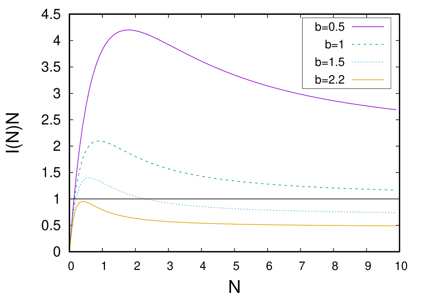
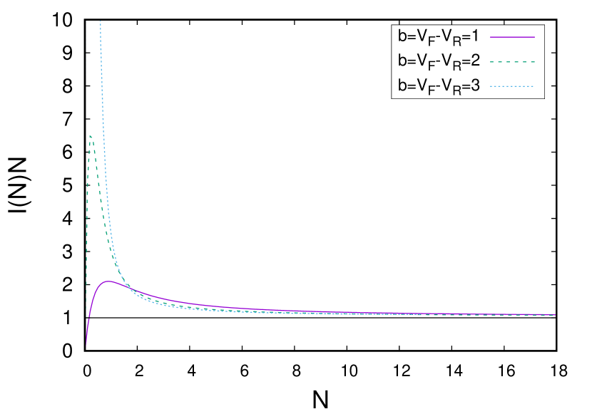
Figure 1: Number of steady states depending on the connectivity parameter $\mathbf{b}$. Intersections between function $I(N)N$ and the straight line one provide the stationary firing rates of the Fokker-Planck equation (8). Left: Function $I(N)N$ for fixed values: $V_{F}=2$, $V_{R}=1$ and $a=1$ and different values of the connectivity parameter $b$. Right: Function $I(N)N$ for values of connectivity parameter exactly the distance between $V_{F}$ and $V_{R}$. $V_{R}=1$ and $V_{F}$ takes the values $\{2,3,4\}$.

For every value of $b$, simulations have been performed with and without delay, as well as using the cascade mechanism when the physical solution makes sense. In the simulations, unless otherwise indicated, we consider the following fixed values: 80000 neurons, i.e., $\mathcal{N}=80000$, $a=1$, $V_{R}=1$ and $V_{F}=2$.

4.1 Physical solutions: $b<V_{F}-V_{R}$

In this section we describe the behaviour of the physical solutions of the model. We also compare the results with those obtained for the delayed system and for the Fokker-Planck description. We recall that in this case there is a unique stationary solution (see Fig.1) and the solutions can explode in a finite time, if the initial data is highly concentrated around the threshold potential [5]. We numerically study these two properties of the model for the particle system.

We consider $b=0.5$ in our simulations (the behaviour for different values of $b$ is qualitatively equivalent), and two different kind of initial data, whose histograms are described in Fig.2. These histograms show the initial distribution through which we order the $80000$ neurons that compose the particle system, depending on the value of their membrane potential. In the left plot we consider a normal distribution with $\nu_{0}=0$ and $\sigma^{2}=0.25$. We consider this initial condition for simulations which describe global existence situations. While in the right plot, we consider a normal distribution with $\nu_{0}=1.83$ and $\sigma=0.003$, placed very close to the threshold potential ($V_{F}=2$). This initial condition is used to study the blow-up phenomenon.

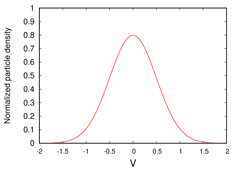
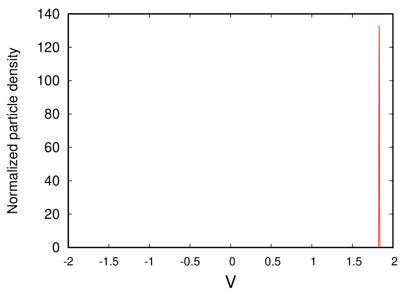
Figure 2: Two initial distributions of the particle system. Left: normal distribution with $\nu_{0}=0$ and $\sigma^{2}=0.25$. Right: normal distribution with $\nu_{0}=1.83$ and $\sigma=0.003$.

4.1.1 Convergence to the stationary solution

We consider the initial datum which is far from $V_{F}$, Fig.2 Left, and the algorithm for classical solutions described in Sect.3. Fig.3 shows the evolution in time of the solution until it reaches the steady state.

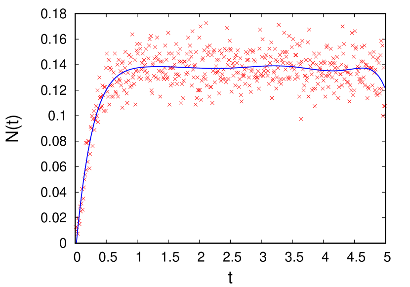
(a)

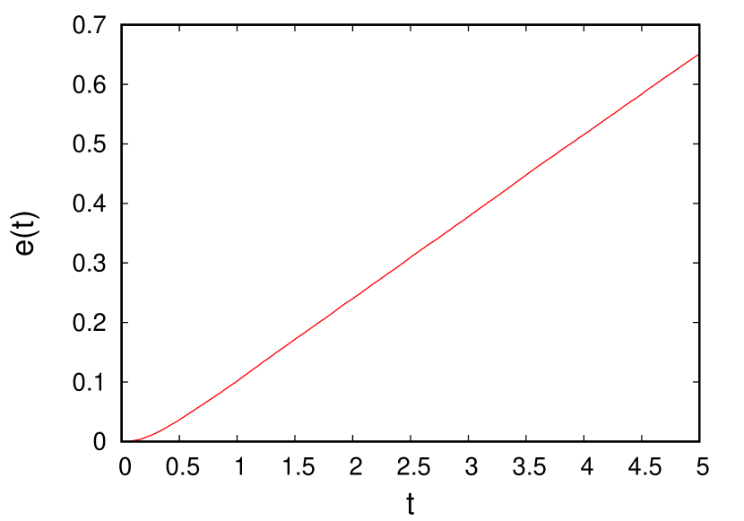
(b)

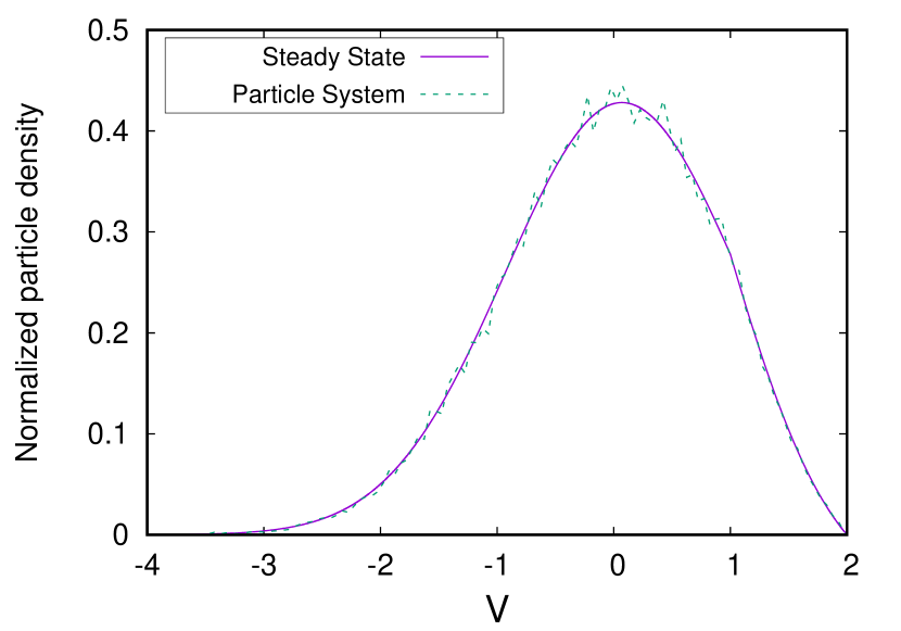
(c)

Figure 3: Convergence to the steady state. $\mathbf{b=0.5}$. The initial condition is a normal distribution with $\nu_{0}=0$ and $\sigma^{2}=0.25$. (a) Time evolution of the firing rate. (b) Time evolution of the expectation. (c) Particle voltage distribution at final time $5$ in comparison with the stationary solution of Fokker-Planck equation.

We observe a very sparse firing rate value, Fig.3(a), whose arithmetic mean is around the value $0.14$, in accordance with the value found for the Fokker-Planck equation [5]. Fig.3(b) shows the evolution of the expectation along the simulation. At the beginning the expectation remains almost zero, because the initial condition guarantees that there are not neurons spiking. After that the expectation increases due to the effect of the diffusion. The distribution of the voltage values at the end of the simulation is shown in Fig.3(c) compared to the the stationary solution of Fokker-Planck equation given in [5].

4.1.2 Blow-up phenomenon

To describe the blow-up phenomenon we consider the initial datum given in Fig.2 Right, and, as first step, the algorithm for classical solutions (see Sect.3). The evolution in time of the solution is described in Fig.4. Figs.4(a) and 4(b) show that blow-up occurs at the beginning of the simulation, the firing rate increases very fast. At blow-up time the expectation is set to $1$, which means that all neurons have already spiked, sense in which we understand the blow-up phenomenon. After that the increasing rate of the expectation decreases.

In Fig.4(a) we see how the firing rate increases very fast to its maximum value, and then decreases to the stationary value. Figs.4(c) and 4(d) show the singularity that occurs during the blow-up time, when the derivative of the expectation, i.e., the firing rate, becomes infinity for the mean field limit. After that, the expectation shows that every neuron has spiked and then it grows slowly. In the Fig.4(e), we observe the value of the voltages distribution before and after the blow-up phenomenon. The distribution at $t=0.004$ is obtained before almost all the neurons spike at once. After that, the distribution shows a very singular shape ($t=0.0046$), to subsequently becomes more regular and evolves to the steady state.

Therefore, Fig.4 shows that the particle system continues after the blow-up and converges to the unique stationary distribution (see Fig.4(f)). In this process, the notion of a classical solution is lost, since the expectation has a jump and therefore, the solution really becomes physical. After the synchronization of the system (explosion time), the expectation becomes continuous again and the system evolves towards the steady state, in a classical way.

4.1.3 Cascade mechanism

To better understand the notion of physical solution, we repeat the previous experiment considering the cascade mechanism (see Sect.3). We observe that the behaviour of the particle system is very similar with both approaches. In Figs.5(a) and 5(b) the firing rate and the expectation perform a similar behaviour to the blow-up one described with the algorithm without cascade mechanism. The voltages distribution before and after the blow-up, Fig.5(c), are also similar to the one showed before. After that, the system stabilizes to the unique steady state (see Fig.5(d)).

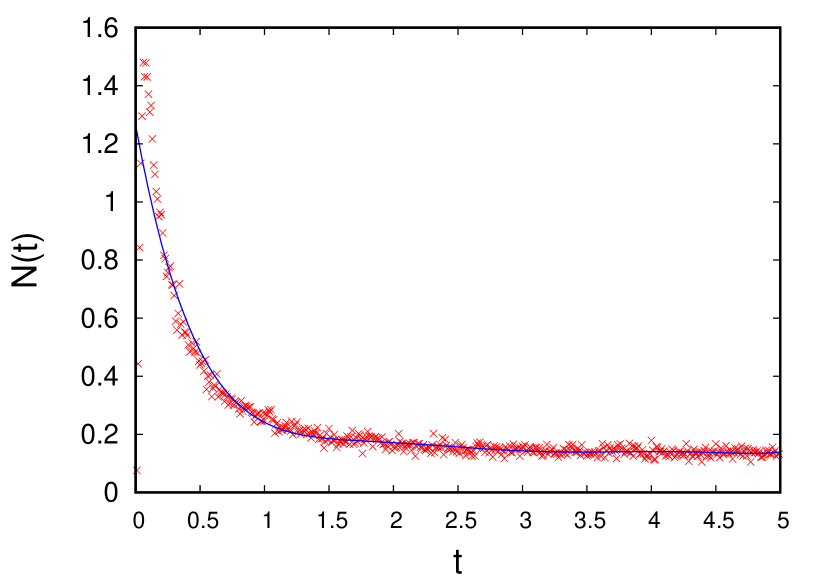
(a)

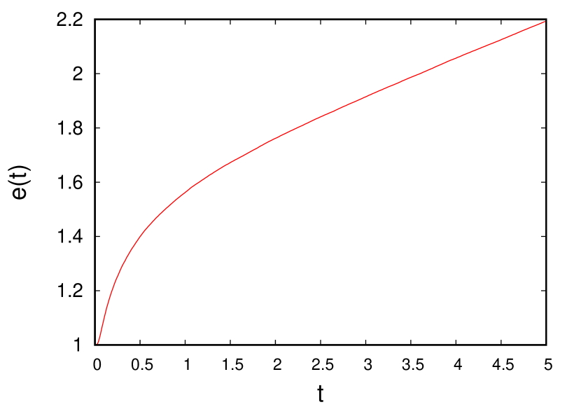
(b)

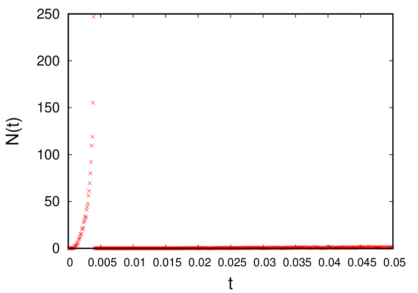
(c)

(d)

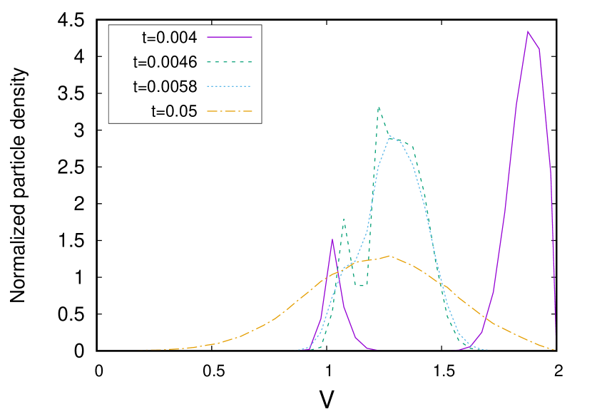
(e)

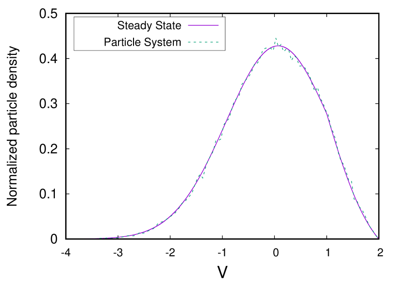
(f)

Figure 4: Blow-up phenomenon with classical approach. $\mathbf{b=0.5}$. The initial condition is a normal distribution with $\nu_{0}=1.83$ and $\sigma=0.003$. (a) Time evolution of the firing rate. (b) Time evolution of the expectation. (c) Time evolution of the firing rate before and after the blow-up. (d) Time evolution of the expectation before and after the blow-up. (e) Time evolution of the particle voltage distribution before and after the blow-up. (f) Particle voltage distribution at time 5 in comparison with the stationary solution of Fokker-Planck equation.

The main differences between both approaches are observed in Fig.5(e), which describes the values of the voltages distributions in the blow-up time. The distribution with cascade mechanism is shifted to the right, since the reset value is $\tilde{V}_{R}=V\left(t^{-}\right)-\left(V_{F}-V_{R}\right)+b\Delta e(t)$, which is different from $V_{R}$ because $\Delta e(t)\neq 0$. Moreover, we appreciate a group of neurons that has not yet fired, in the "cascade off" picture, while the "cascade on" distribution has completely overtaken the firing threshold. This happens because the cascade mechanism allows neurons to fire at $\tilde{V}_{F}=V_{F}-b\Delta e(t)$. Also the expectation variation is different to the computed in the classical case, since it counts spikes which occur beyond $\Gamma_{0}$ (see Sect.2.1). In particular, the variation of the expectation computed without cascade mechanism was $\Delta e(t)=0.303075$, lower than that calculated in the cascade model, whose value is $\Delta e(t)=0.574662$.

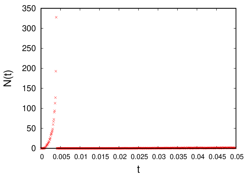
(a)

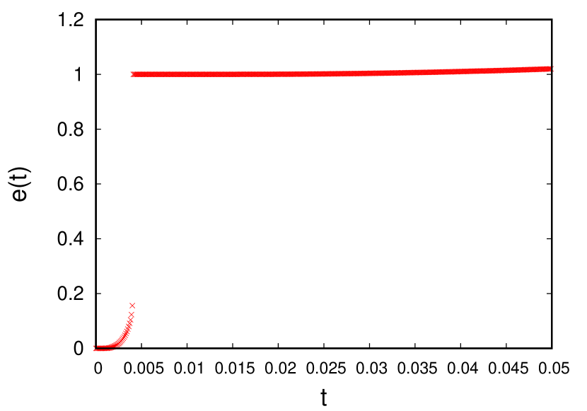
(b)

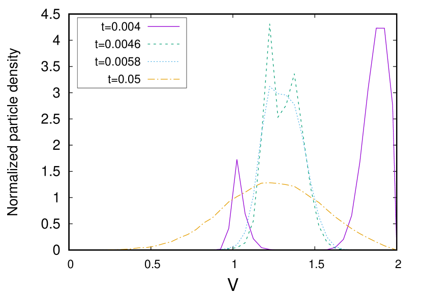
(c)

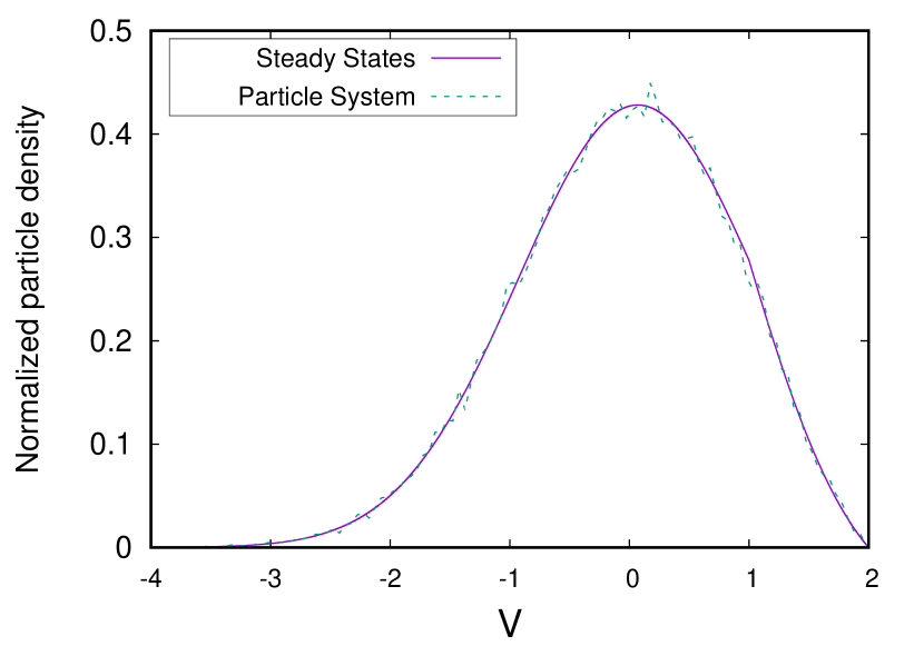
(d)

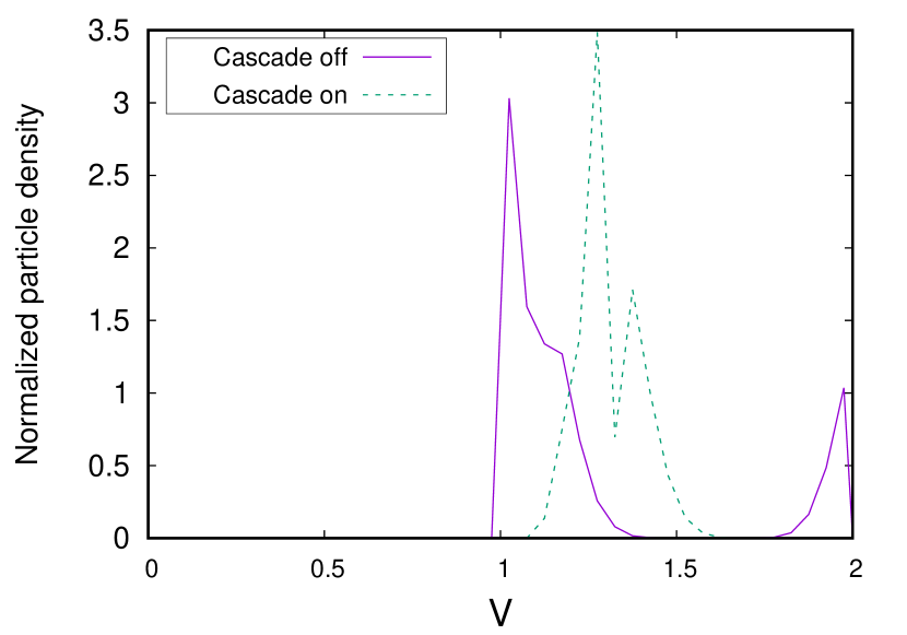
(e)

Figure 5: Blow-up phenomenon with cascade mechanism. $\mathbf{b=0.5}$. The initial condition is a normal distribution with $\nu_{0}=1.83$ and $\sigma=0.003$. (a) Time evolution of the firing rate before and after the blow-up. (b) Time evolution of the expectation before and after the blow-up. (c) Time evolution of the particle voltage distribution before and after the blow-up. (d) Particle voltage distribution at time 5 in comparison with the stationary solution of Fokker-Planck equation. (e) Comparison of the voltage distributions in the blow-up moment with both approaches: with and without cascade mechanism.

4.1.4 Transmission delay

Finally, we analyse how the transmission delay avoids the blow-up phenomenon. With this aim we consider: a normal distribution with mean $\nu_{0}=1.83$ and standard deviation $\sigma=0.003$, as initial distribution; and three different transmission delays: $\delta=0.1$, $\delta=0.01$ and $\delta=0.001$.

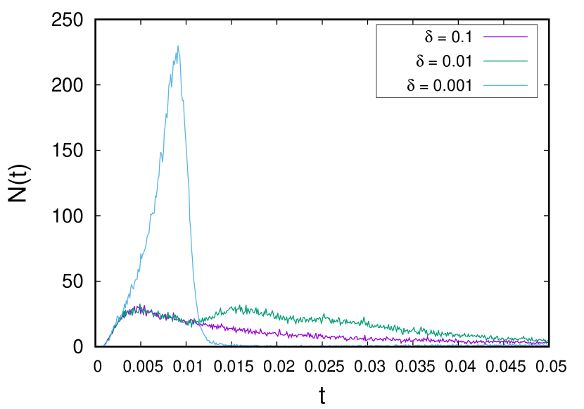
(a)

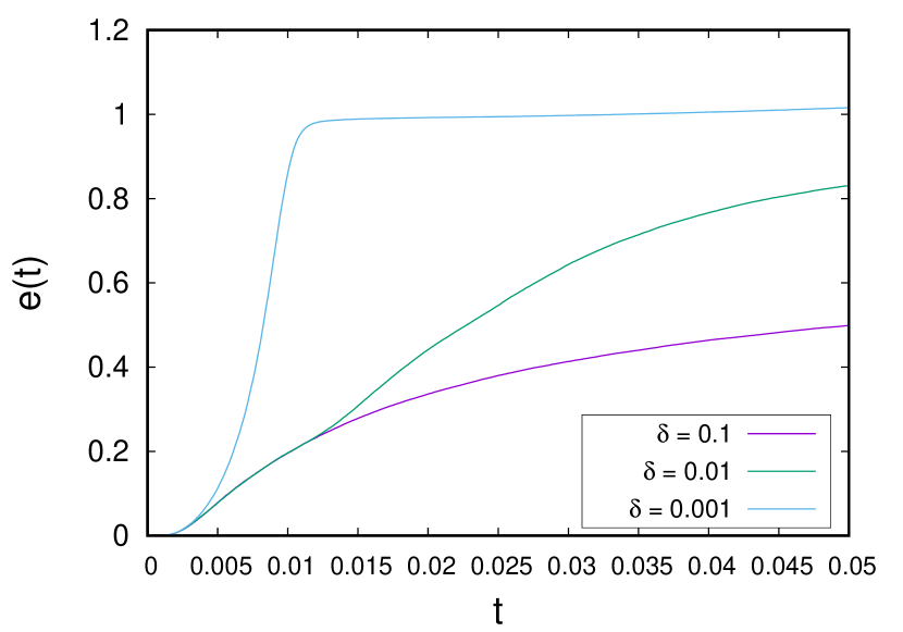
(b)

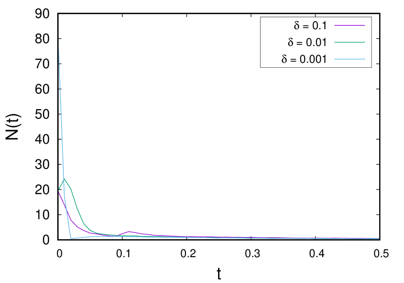
(c)

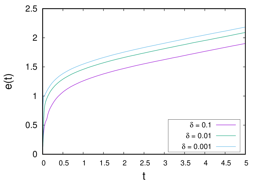
(d)

Figure 6: Blow-up situation with delay. $\mathbf{b=0.5}$. The initial condition is a normal distribution with $\nu_{0}=1.83$ and $\sigma=0.003$. We considered different values for the delay. (a) Time evolution of the firing rate until 0.05. (b) Time evolution of the expectation until 0.05. (c) Time evolution of the firing rate until time 0.5. (d) Time evolution of the expectation until time 5.

Fig.6 shows that neurons achieve managing to dodge the blow-up phenomenon, because the firing rate and the expectation prevent the singularities with the transmission delay. In Fig.6(a) we observe how the firing rate increases until it reaches its maximum value and then decreases. Therefore, the expectation does not present any singularity, see Fig.6(b), and the solution is classical. However, if $\delta\to 0$ the firing rate diverges in finite time, because its maximum value is higher when the value of the transmission delay is reduced, and the solution will be physical, instead of classical. In the long time behaviour, the firing rates converge to the stationary value, see Fig.6(c), since the growth rates of the expectation are the same, Fig.6(d). As a consequence, the system converges to the unique steady state.

4.2 Non-physical solutions $b>V_{F}-V_{R}$

In this section we focus on the case $b>V_{F}-V_{R}$, where the notion of physical solutions does not make sense, since the neuronal network is strongly excitatory and neurons could fire more than one spike at the same time (see Remark 2.3). We remember that for this range of values of $b$, the system has two steady states or none (see Fig.1). We describe both situations with $b=1.5$ (two steady states) and $b=2.2$ (no steady states).

4.2.1 Case with two steady states. Connectivity parameter $\mathbf{b=1.5}$

For $b=1.5$, the long time behaviour for Fokker Planck Equation solutions was numerically studied in [5]: the steady state with lowest firing rate is stable, while the higher one is unstable, and the network explodes at finite time for certain initial conditions. Here we reproduce these phenomena at the level of the particle system. We discover that the particle system, in cases where blow-up occurs, tends to a "plateau distribution" if we consider a transmission delay.

Convergence to the stationary solution with the lowest firing rate.- Let us consider two different initial conditions for the particle system voltages, which are far from the threshold $V_{F}$, (see Fig.7(a)): a normal distribution with $\nu_{0}=0$ and $\sigma^{2}=0.25$, and the profile given by

$$p(v)=\frac{F_{rate}}{a}e^{-\frac{\left(v-bF_{rate}\right)^{2}}{2a}}\int_{max(v,V_{R})}^{V_{F}}e^{\frac{\left(w-bF_{rate}\right)^{2}}{2a}}dw$$ (16)

with $F_{rate}=2.31901$, which approximates the highest stationary firing rate. The profile (16) is an approximation of the steady state for the Fokker-Planck equation with the highest firing rate (see [5] for details).

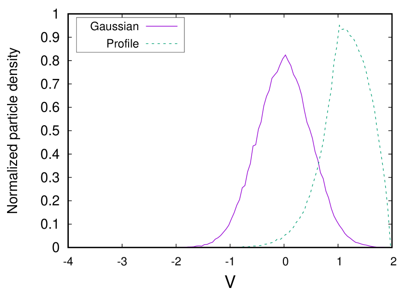
(a)

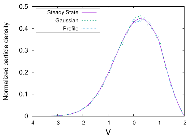
(b)

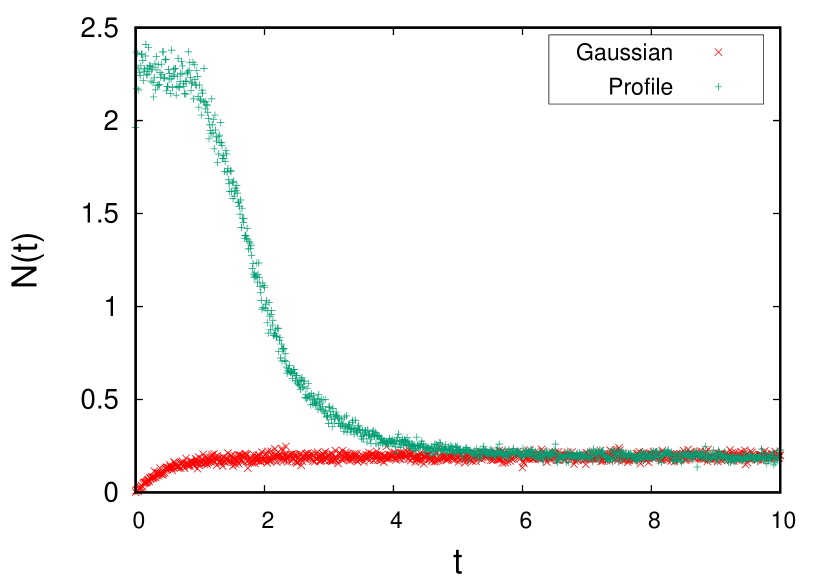
(c)

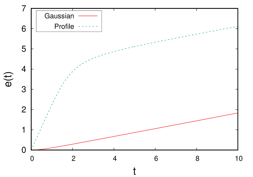
(d)

Figure 7: Convergence to the lowest steady state. $\mathbf{b=1.5}$. The initial condition is a normal distribution with $\nu_{0}=0$ and $\sigma^{2}=0.25$ in the "Gaussian" case and a profile distribution given by Eq.(16) in the "Profile" one. (a) Initial conditions used in the simulations. (b) Particle voltage distributions at time $5$ in comparison with the lowest steady state of Fokker-Planck equation. (c) Time evolution of the firing rate. (d) Time evolution of the expectation.

In the first case, where the initial condition is a normal distribution, the particle system tends to the steady state with lowest firing rate value, see Fig.7(b). The evolution over time is described in terms of the firing rate in Fig.7(c), and also through the expectation in Fig.7(d). The firing rate evolves towards the lowest stationary value, and therefore, the expectation presents a linear growth at the end of the simulation.

To describe the unstability of the steady state with the highest firing rate value, we consider the second initial datum, profile (16). In Fig.7(b), we see that the distribution of voltages ends up in the same steady state as in the previous case. Simulations starting with the profile (16) and a little increase of the value $F_{rate}$ produce the explosion in finite time, as in [5]. Therefore, based on our results, and results in [5], the steady state with the highest firing rate appears to be a “limit state” between situations of convergence towards the lowest steady state and those of blow-up.

Blow-up phenomenon.- We consider an initial condition given by a normal distribution with $\nu_{0}=1.83$ and $\sigma=0.003$ (Fig.2 Right), and we show the data obtained during the simulation in Fig.8.

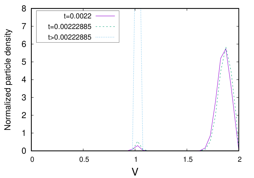
(a)

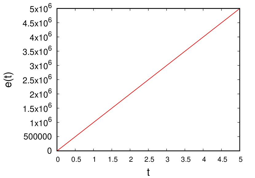
(b)

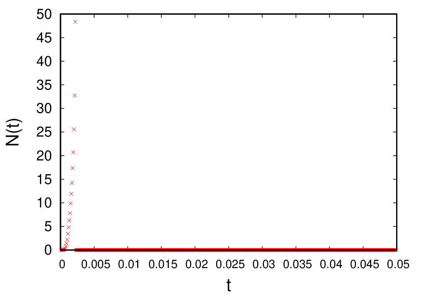
(c)

Figure 8: Blow-up phenomenon. $\mathbf{b=1.5}$. The initial condition is a normal distribution with $\nu_{0}=1.83$ and $\sigma=0.003$. (a) Time evolution of the particle voltage distribution before and after the blow-up. (b) Time evolution of the expectation. (c) Time evolution of the firing rate.

After a short period of time, almost all neurons spike simultaneously (blow-up phenomenon). Then neurons reset their voltages to the value $V_{R}$. However, the variation of the expectation computed in the blow-up time is so large that the whole network can spike again in the next step. This means that, if blow-up occurs at time $t_{j-1}$, then $b\frac{n^{j}}{\mathcal{N}}>V_{F}-V_{R}$, due to the high value of the connectivity parameter $b$. This phenomenon causes the system to be in a constant state of blow-up and reset, which we call “trivial solution”. In Fig.8(a) we observe the voltages distributions obtained before and after the blow-up. The final value of the voltage distribution shows that all neurons are locate in $V_{R}$. So that “trivial solution” appears to be a Dirac delta at $V_{R}$, because neurons reset to $V_{R}$ at blow-up time. Consequently, in Fig.8(b) we see that the final value of the expectation is near to $T/\Delta t=5\times 10^{6}$, which is the value that expectation would reaches if all neurons spike in each step from beginning to end of the simulation. In Fig.8(c) we see clearly the moment when the firing rate diverges.

Transmission delay.- We analyse here what happens in the blow-up situation, when transmission delays are taken into account and the system avoids the explosion. We consider the initial datum given in Fig.2 Right and develop several simulations with different transmission delay values: $\delta=0.1$ and $\delta=0.01$. In Fig.9 we show both simulations. With a transmission delay the voltage distribution avoids blow-up and it converges to a new state. We have called to this state "plateau distribution", see Figs.9(c) and 9(d). In this new distribution almost all neurons voltages are located between $V_{R}$ and $V_{F}$. Moreover, the probability to find any voltage in $v\in\left[1,2\right)$ is almost the same.

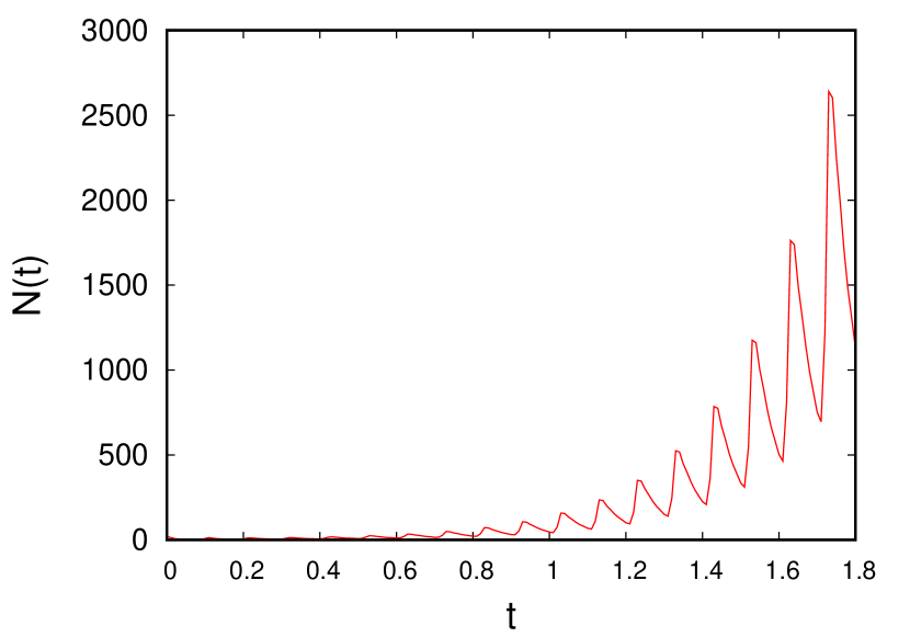
(a)

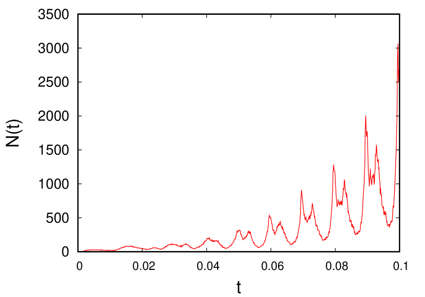
(b)

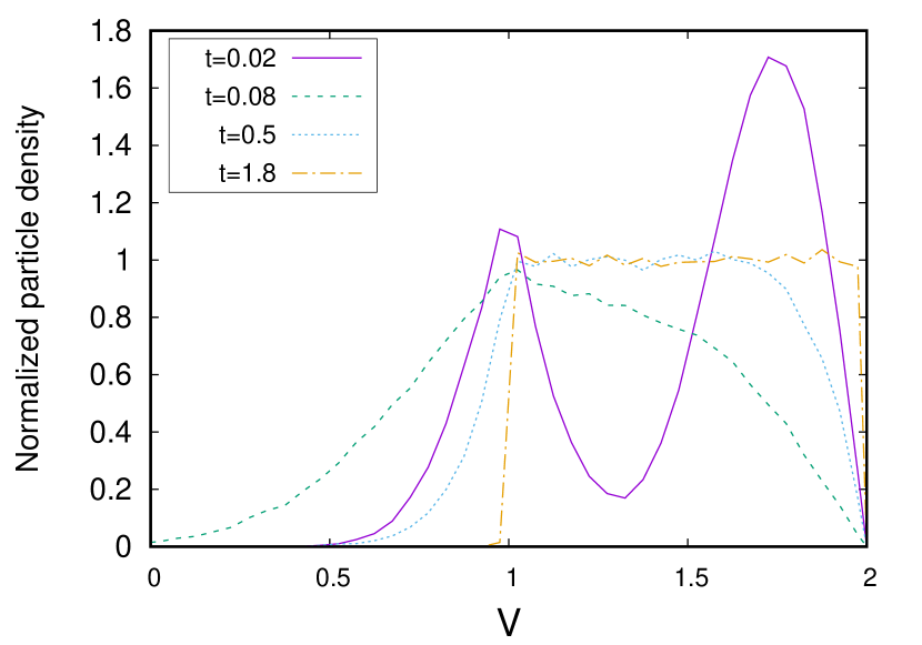
(c)

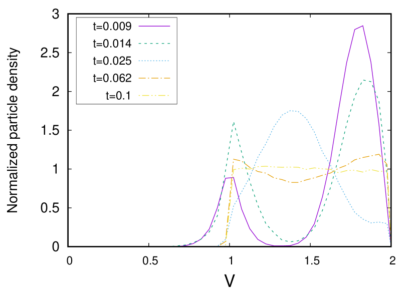
(d)

Figure 9: Blow-up situation with delay. $\mathbf{b=1.5}$. The initial condition is a normal distribution with $\nu_{0}=1.83$ and $\sigma=0.003$. On the left $\delta=0.1$. On the right $\delta=0.01$. (a) and (b) Time evolution of the firing rate. (c) and (d) Time evolution of the particle voltage distribution.

In both simulations, see Figs.9(a) and 9(b), the firing rates tend to increase. This behaviour is in full agreement with the formation of the “plateau” distributions observed in Figs.9(c) and 9(d). On the other hand, the comparison between Figs.9(a) and 9(b) shows the influence of the delay size. As the delay gets smaller and smaller, the firing rate tends to diverge in a finite time. We checked it for $\delta=0.00001$, with which the system does not avoid the blow-up. All neurons spike at once and the distribution converges to the “trivial solution”. Finally, we remark that the time needed to get close to the “plateau” state is directly proportional to the value of the delay, see Figs.9(c) and 9(d).

4.2.2 Case without steady states. Connectivity parameter $\mathbf{b=2.2}$

We also study the case with $b=2.2$, which represents highly excited neural networks that do not exhibit stationary states (see Fig.1). In Fig.10 we can observe that the blow-up is guaranteed regardless of the initial conditions, without transmission delay (see [36]). In that simulation the initial distribution is far from the firing threshold and the firing rate diverges in finite time. On the right side of the figure we see the last output for the distribution, before all the neurons fire at once.

When a transmission delay is considered, the system avoids blow-up and converges to a "plateau" state. Fig.11 shows time evolution of the particle system, with an initial distribution close to $V_{F}$ and with a transmission delay value $\delta=0.1$. In this situation, the firing rate increases, but does not diverge in finite time, as we can see in Fig11(a). The firing rate also represents the growth rate of expectation, as shown in Fig.11(b). As in the case $b=1.5$, that behaviour is reflected in the evolution of the potentials distribution. At the beginning of the simulation, Fig.11(c) , we see how the system oscillates between a shape similar to that which occurs without delay and a “plateau” distribution. Some time later, the system approaches the “plateau” distribution, i.e., a uniform distribution in $(V_{R},V_{F})$, Fig.11(d).

This behaviour was observed for Fokker-Planck equation solutions in [10, (Fig.2)], and although the evolution of the solutions was not shown in said article, the construction of the "plateau" distribution was already observed.

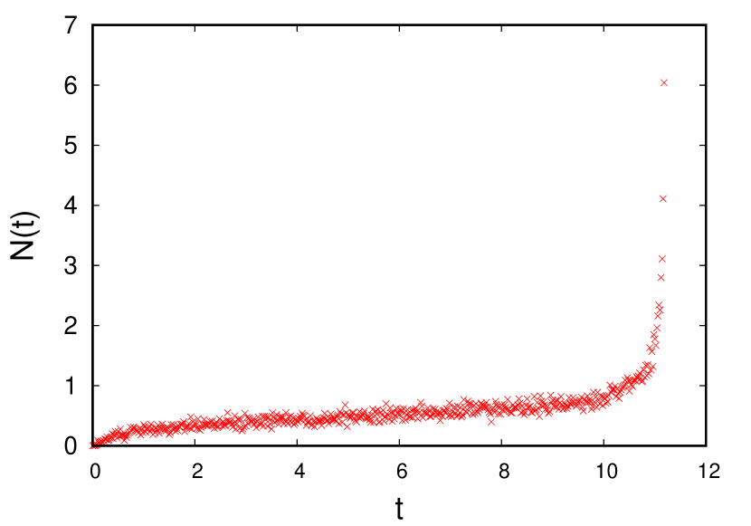
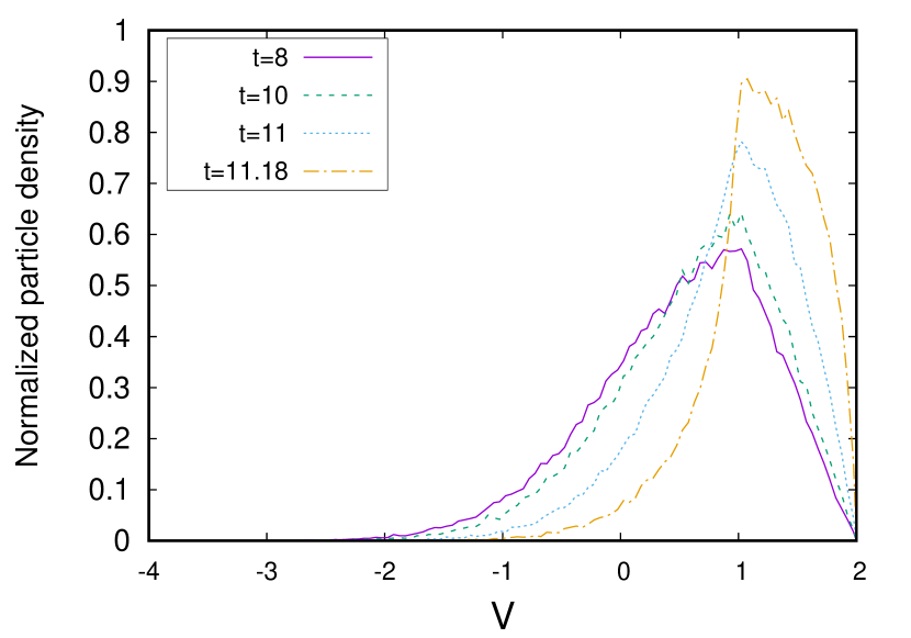
Figure 10: Blow-up phenomenon without delay. $\mathbf{b=2.2.}$ The initial condition is a normal distribution with $\nu_{0}=0$ and $\sigma^{2}=0.25$. Left: Time evolution of the firing rate. Right: Time evolution of the particle voltage distribution before the blow-up.

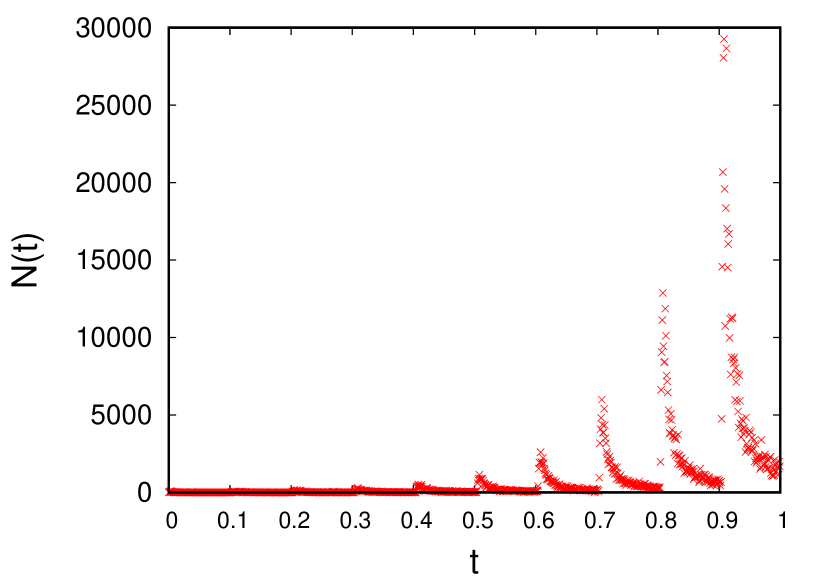
(a)

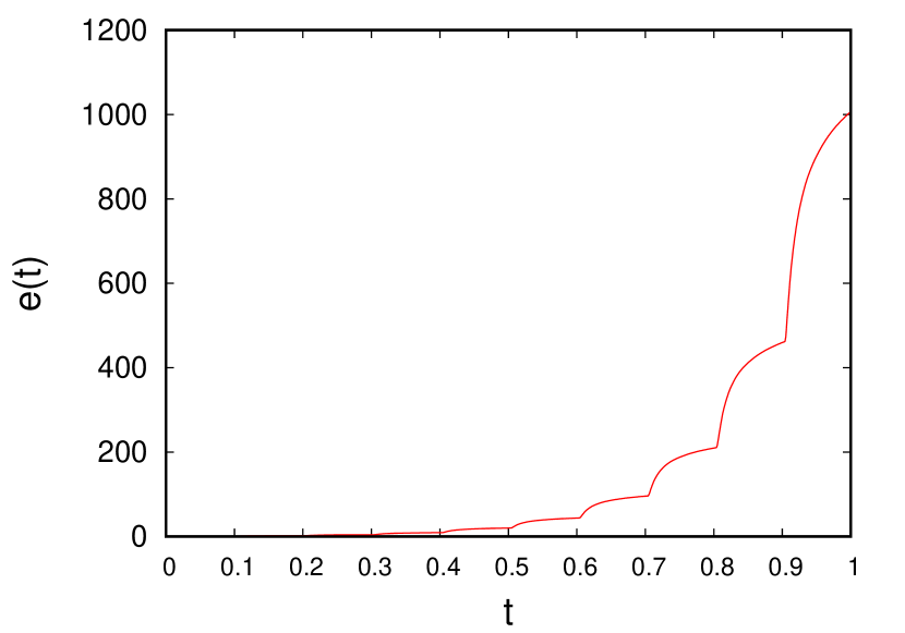
(b)

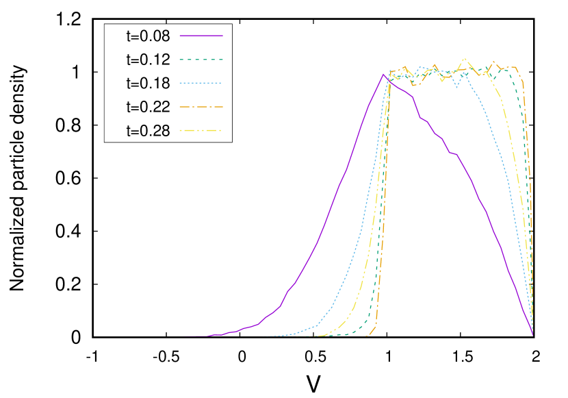
(c)

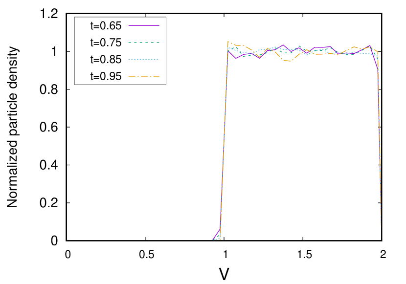
(d)

Figure 11: Blow-up situation with delay. $\mathbf{b=2.2}$. The initial condition is a normal distribution with $\nu_{0}=1.83$ and $\sigma=0.003$, and the delay value $\delta=0.1$. (a) Time evolution of the firing rate. (b) Time evolution of the expectation. (c) and (d) Time evolution of the particle voltage distribution during the formation of the "plateau" state.

4.3 Limiting case $b=V_{F}-V_{R}$

In this section we analyse the limiting case for which the notion of physical solution no longer makes sense (see Sect.2.1). This case is in between of two regimes: for values $b<1$, there is only one steady state (see Fig.1) and simulations show that all neurons in the system can fire at the same time, and then converge towards the steady state (see Sect.4.1). However, if $b>1$, the system needs the transmission delay to avoid the explosion, because the physical solutions do not make sense (see Sect.4.2). For $V_{F}=2$ and $V_{R}=1$, the limiting value of the connectivity parameter is $b=1$. For this value of $b$, neurons can spike twice if their membrane potentials are close to $V_{F}$. Therefore, we focus on studying this case through the delayed and non-delayed algorithms, without cascade mechanism. As first test, we checked the convergence to the unique stationary state, starting with a distribution of neurons with membrane potentials far from the threshold value. We skip these figures here, and concentrate on the results found for possible explosion situations. Throughout this section, the initial condition will be always a normal distribution with mean $\nu_{0}=1.83$ and variance $\sigma=0.003$ (see Fig.2).

The delayed system approximates the solution of the particle system as the transmission delay $\delta$ tends to zero. With this purpose, we have made the comparison of the non-delayed system with the sufficiently low delayed one ($\delta=0.0001$) in Fig.12.

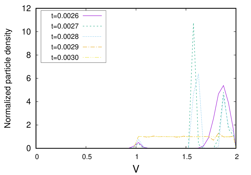
(a)

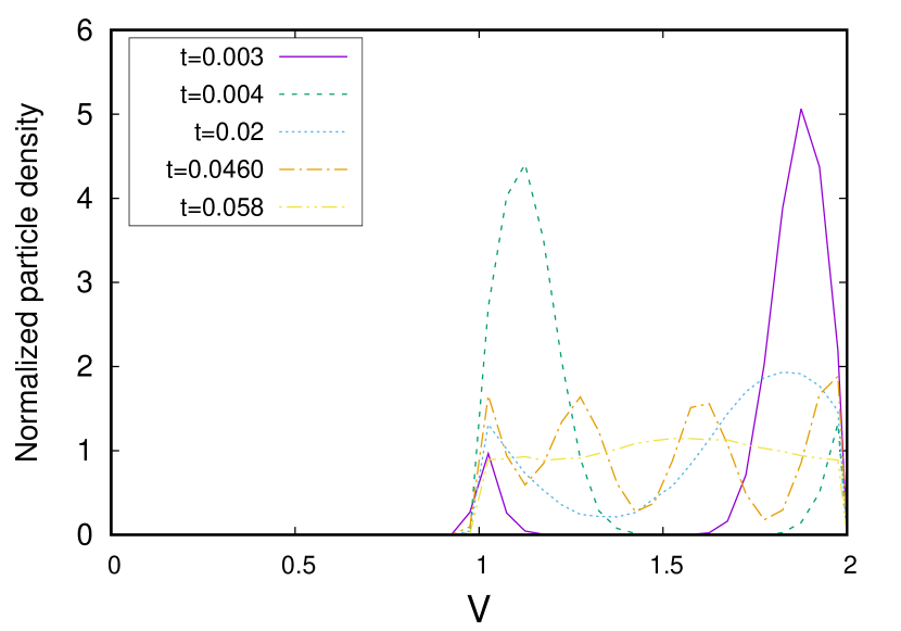
(b)

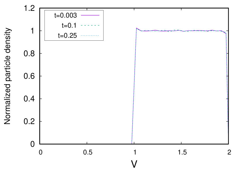
(c)

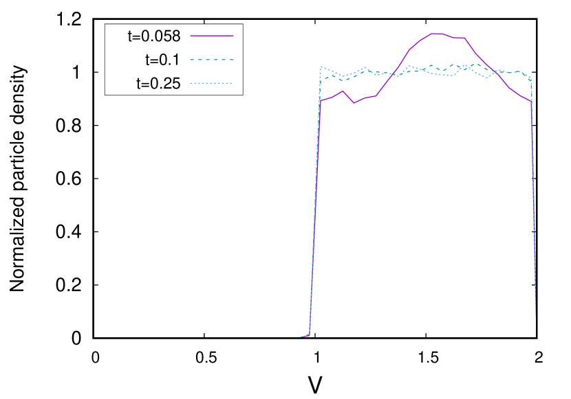
(d)

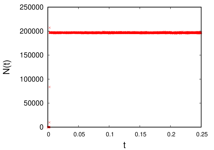
(e)

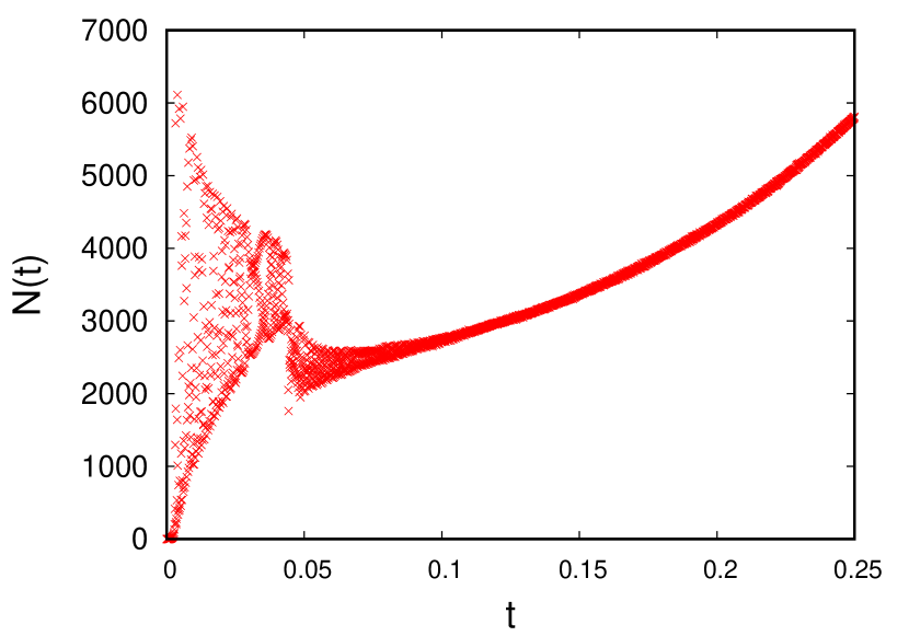
(f)

Figure 12: Time evolution of a particle system without transmission delay and with a very small delay $\mathbf{\delta=0.0001.}$ $\mathbf{b=1.}$ The initial condition is a normal distribution with $\nu_{0}=1.83$ and $\sigma=0.003$ in both simulations. (a) Time evolution of the particle voltage distribution without delay. (b) Time evolution of the particle voltage distribution with delay. (c) Time evolution of the particle voltage distribution without delay. (d) Time evolution of the particle voltage distribution with delay. (e) Time evolution of the firing rate without delay. (f) Time evolution of the firing rate with delay.

For the non-delayed case, we observe in Fig.12(a) how the voltages distribution approaches the firing threshold and the system achieves the "plateau" state, which appears to be a stable state, as shown in Fig.12(c). The transition between all neurons firing at once and the “plateau” distribution occurs extremely quickly. However, the delayed system oscillates further until it approaches the “plateau” distribution (see Fig.12(b)). This “plateau” state seems to be also stable as shown in Fig.12(d). The dynamics of the firing rates can be seen in the bottom of Fig.12. In the non-delayed case, the firing rate remains constant from almost the beginning in a very high value (see Fig.12(e)). This means that the system has converged towards the “plateau” distribution, and that value is an approximation of an infinite firing rate. In the case with delay the firing rate undergoes oscillations prior to the formation of the “plateau” (see Fig.12(f)). Later, once the “plateau” is formed, its value tends to grow. In the long term it should reach the value of the non-delayed case, which would give a more defined form to the “plateau”.

We have also studied the effect of higher values of delay for blow-up situations. As the delay value increases, the “plateau” state becomes unstable and the system tends to the unique steady state, as shown in Fig.13. For the lower values $\delta=0.001$ and $\delta=0.01$ the system remains close to the "plateau" distribution for a while. However, for $\delta=0.1$, the system does not even come close to the "plateau" state, see Figs.13(a) and 13(b). Finally, Fig.13(c) shows how the system tends to the steady state for the three delay values considered, even for the lowest ones, for which the system was close to the “plateau” state.

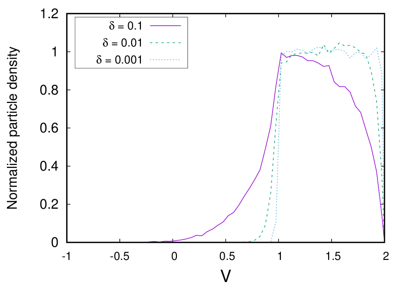
(a)

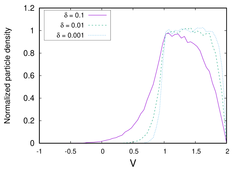
(b)

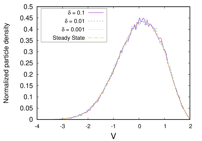
(c)

Figure 13: Time evolution of a particle system with high transmission delays. $\mathbf{b=1}$. The initial condition is a normal distribution with $\nu_{0}=1.83$ and $\sigma=0.003$ in all simulations for different delays. (a) Particle voltage distribution at time $t=0.0012$ with different delay values. (b) Particle voltage distribution at time $t=0.0025$ with different delay values. (c) Particle voltage distribution at time $t=5$ with different delay values compared to the steady state of the Fokker-Planck equation.

4.4 Plateau formation

In this section we try to understand the formation of the observed “plateau” distributions. Additionally, we propose a possible explanation of that behaviour.

Fig.14 shows the comparison of the “plateau” distributions found for $b=1.5$ and $b=2.2$, and the following profiles:

$$p(v)=\frac{\tilde{N}}{a}e^{-\frac{\left(v-bN\right)}{2a}}\int_{max(v,V_{R})}^{V_{F}}e^{\frac{\left(w-bN\right)^{2}}{2a}}dw,\quad N\in\mathbb{R}^{+},$$ (17)

where $\tilde{N}=a\left(\int_{-\infty}^{V_{F}}e^{-\frac{\left(v-bN\right)}{2a}}\int_{max(v,V_{R})}^{V_{F}}e^{\frac{\left(w-bN\right)^{2}}{2a}}dwdv\right)^{-1}$, which guarantees the conservation law: $\int_{-\infty}^{V_{F}}p(v)dv=1$. There is a high coincidence between the “plateau” distributions and the profiles (17) as $N$ increases. Furthermore, the dynamics of the particle system appears to go through states with the form (17) with increasing $N$, during the formation of its “plateau” states (for instance, see Fig.11(c)).

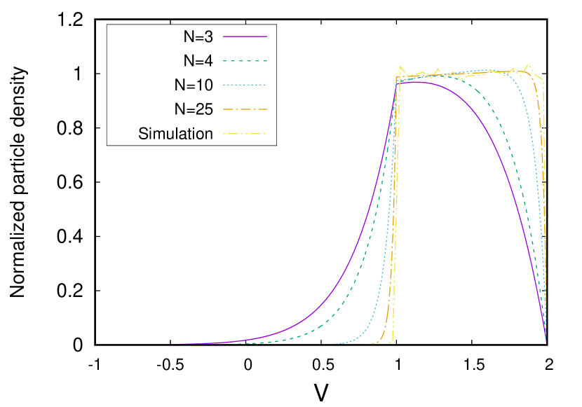
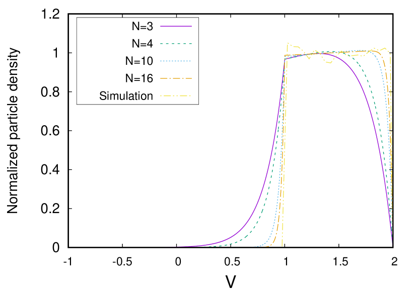
Figure 14: Comparison of “plateau” distributions with profiles (17). Left: $b=1.5$. Right: $b=2.2$.

On the other hand, we know that steady states of the Fokker-Planck equation are profiles (17) as long as $\tilde{N}=N$, which is exactly the Eq.(3.6) in [5]. That is, the implicit equation $NI(N)=1$, with $I(N)=a^{-1}\int_{-\infty}^{V_{F}}e^{-\frac{\left(v-bN\right)}{2a}}\int_{max(v,V_{R})}^{V_{F}}e^{\frac{\left(w-bN\right)^{2}}{2a}}dwdv$. Therefore, for any $N$ that is not a solution of that implicit equation, the profile (17) is not a stationary distribution of the system. As a consequence, the profiles shown in Fig.14 are not stationary states. For $b=1.5$ (left plot) there are two steady states, but neither corresponds to the values shown in that figure, and for $b=2.2$ (right plot) there are no stationary solutions.

Therefore, the question is: does the system evolve towards profiles (17) with $N$ tending to infinity? Based on our results, we think the answer could be afirmative, because:

• For the delayed systems, Figs.9 and 11 show that the particle system appears to tend to different profiles (17), during the time intervals $J_{m}=\left(m\,\delta,(m+1)\,\delta\right)$, with $m\in\mathbb{N}$. In these intervals, the system seems to evolve towards "pseudo-stationary" states that verify the equation

  $$\frac{\partial}{\partial v}\left[(v-bN_{\delta}^{m})p_{m}+a\frac{\partial}{\partial v}p_{m}(v)+\tilde{N}_{\delta}^{m}H(v-V_{R})\right]=0,$$

  for certain values $N_{\delta}^{m}$ and $\tilde{N}_{\delta}^{m}$. Thus, taking into account the boundary conditions, we integrate the equation and find that

  $$p_{m}(v)=\frac{\tilde{N}_{\delta}^{m}}{a}e^{-\frac{(v-bN_{\delta}^{m})^{2}}{2a}}\int_{\max(v,V_{R})}^{V_{F}}e^{\frac{(w-bN_{\delta}^{m})^{2}}{2a}}\,dw,$$ (18)

  which corresponds to (17). In certain sense, we can understand $N_{\delta}^{m}$ as an approximation of a “pseudo-stationary” firing rate in the delay time.

• Moreover, Fig.9(a) and Fig.11(a) show how the firing rates increase over time. This also causes the sequences of $N_{\delta}^{m}$ and $\tilde{N}_{\delta}^{m}$ values to increase. As a result, profiles (18) look more and more like a “plateau” distribution, since $\lim_{N_{\delta}^{m}\to\infty}p_{m}(v)=\frac{1}{V_{F}-V_{R}}H(v-V_{R})$, for $v<V_{F}$.

• In the case $b=1$ we also find a “plateau” distribution in the blow-up situations (see Fig.12), even without the presence of transmission delay. In this case, there is only one steady state with finite firing rate. However, $b=1$ is the only connectivity value with which $\lim_{N\to\infty}NI(N)=1$ (see Fig.1 Left and [5]). The last statement leads us to think that profile (17) with $N\to\infty$, i.e. $\tilde{p}(v):=\frac{1}{V_{F}-V_{R}}H(v-V_{R})$ for $v<V_{F}$ and $\tilde{p}(V_{F}):=0$, is also a stationary solution. Although it would not be in the classical sense, since $\tilde{p}(V_{R}^{-})\neq\tilde{p}(V_{R}^{+})$.

5 Conclusions

In this work we have made progress on the path towards a better understanding of the NNLIF models. We have numerically analysed the particle system that originates these models. First, we have validated our numerical scheme by comparing our results with those obtained for the Fokker-Planck equation in [5, 10, 8]. After which, we have discovered new properties of the solutions. Specifically, we have shown what happens to the particle system when the blow-up phenomenon occurs in a finite time. We have discovered that system behaviour after the blow-up depends on the connectivity parameter $b$:

• For weakly connected systems, that is, $b<V_{F}-V_{R}$, the system overcomes the explosion and tends to its unique steady state. This fact is in agreement with the global existence theory and with the notion of physical solution, instead of classical one [16]. At the instant of the explosion, the firing rate diverges, but in such a way that the singularity of the expectation is controlled. Then the neurons tend to the equilibrium distribution of the system.

• For highly connected systems, understood as $b\geq V_{F}-V_{R}$, the concept of physical solution no longer makes sense, because neurons can fire twice at the same time. For this range of values, the system presents a wealth of properties, since it can have one, two or none steady state. Our numerical results show that:

  • In situations where the blow-up would occur in a finite time, the system tends to a “plateau” distribution when synaptic delays are taken into account. That happens even with an initial distribution far from the threshold potential, in cases where there are no steady states.

  • When the system exhibits two steady states, only the one with the lowest firing rate is stable, as shown in [5]. But our results also seem to indicate that “plateau” distributions are stable, when transmission delay is taken into account. Therefore, the system would exhibit bistability between the steady state with the lowest firing rate and the “plateau” distribution.

  • The limiting case $b=1$ is especially interesting because the “plateau” profile (17) coincides with the stationary profile, with $N\to\infty$. Our results indicate that the system evolves to a "plateau" distribution under blow-up situations, either without synaptic delay or with a very small delay value. Nevertheless, for a high enough delay the system avoids blow-up and tends to the stationary state, instead of the “plateau”.

From a neurophysiological point of view, the explosion phenomenon can be understood as the synchronization of the neural network, where all neurons spike at once. This phenomenon occurs if synaptic delay is not taken into account. However, when some transmission delay is included in the model, we show that the system moves into an asynchronous state (stationary distribution away from the threshold value) or towards a “plateau” distribution, which means that the membranes potential tend to be uniformly distributed in the interval $(V_{R},V_{F})$. The system seems to evolve towards these “plateau” distributions, passing near the “pseudo equilibria” caused by the transmission delay. The limiting case $b=1$ has a “pseudo equilibrium” associated with $N\to\infty$, that matches the profile of a “limit steady-state” (with $N\approx\infty$). In this case, the “plateau” distribution is obtained without the need to include any transmission delay. The rigorous demonstration of the conjectures arising from our results is posed as future work.

The authors acknowledge support from projects MTM2017-85067-P of Spanish Ministerio de Economía, Industria y Competitividad and the European Regional Development Fund (ERDF/FEDER).

References

- [1] Acebrón, J., Bulsara, A., and Rappel, W. J. Noisy Fitzhugh-Nagumo model: From single elements to globally coupled networks. Physical Review E 69, 2 (2004), 026202.
- [2] Brette, R., and Gerstner, W. Adaptive exponential integrate-and-fire model as an effective description of neural activity. Journal of neurophysiology 94 (2005), 3637–3642.
- [3] Brunel, N. Dynamics of sparsely connected networks of excitatory and inhibitory spiking neurons. Journal of computational neuroscience 8, 3 (2000), 183–208.
- [4] Brunel, N., and Hakim, V. Fast global oscillations in networks of integrate-and-fire neurons with low firing rates. Neural computation 11, 7 (1999), 1621–1671.
- [5] Cáceres, M. J., Carrillo, J. A., and Perthame, B. Analysis of nonlinear noisy integrate & fire neuron models: blow-up and steady states. The Journal of Mathematical Neuroscience 1, 1 (2011), 7.
- [6] Cáceres, M. J., Carrillo, J. A., and Tao, L. A numerical solver for a nonlinear fokker-planck equation representation of neuronal network dynamics. J. Comp. Phys. 230 (2011), 1084–1099.
- [7] Caceres, M. J., and Perthame, B. Beyond blow-up in excitatory integrate and fire neuronal networks: refractory period and spontaneous activity. Journal of theoretical biology 350 (2014), 81–89.
- [8] Cáceres, M. J., Roux, P., Salort, D., and Schneider, R. Global-in-time solutions and qualitative properties for the nnlif neuron model with synaptic delay. Communications in Partial Differential Equations 44, 12 (2019), 1358–1386.
- [9] Cáceres, M. J., and Schneider, R. Blow-up, steady states and long time behaviour of excitatory-inhibitory nonlinear neuron models. Kinetic & Related Models 10, 3 (2017), 587.
- [10] Cáceres, M. J., and Schneider, R. Analysis and numerical solver for excitatory-inhibitory networks with delay and refractory periods. ESAIM: Mathematical Modelling and Numerical Analysis 52, 5 (2018), 1733–1761.
- [11] Carrillo, J., Perthame, B., Salort, D., and Smets, D. Qualitative properties of solutions for the noisy integrate & fire model in computational neuroscience. Nonlinearity 25 (2015), 3365–3388.
- [12] Carrillo, J. A., González, M. d. M., Gualdani, M. P., and Schonbek, M. E. Classical solutions for a nonlinear fokker-planck equation arising in computational neuroscience. Comm. in Partial Differential Equations 38, 3 (2013), 385–409.
- [13] Chevallier, J. Mean-field limit of generalized hawkes processes. Stochastic Processes and their Applications 127, 12 (2017), 3870–3912.
- [14] Chevallier, J., Cáceres, M. J., Doumic, M., and Reynaud-Bouret, P. Microscopic approach of a time elapsed neural model. Mathematical Models and Methods in Applied Sciences 25, 14 (2015), 2669–2719.
- [15] Compte, A., Brunel, N., Goldman-Rakic, P. S., and Wang, X.-J. Synaptic mechanisms and network dynamics underlying spatial working memory in a cortical network model. Cerebral cortex 10, 9 (2000), 910–923.
- [16] Delarue, F., Inglis, J., Rubenthaler, S., and Tanré, E. Particle systems with a singular mean-field self-excitation. application to neuronal networks. Stochastic Processes and their Applications 125, 6 (2015), 2451–2492.
- [17] Delarue, F., Inglis, J., Rubenthaler, S., Tanré, E., et al. Global solvability of a networked integrate-and-fire model of mckean–vlasov type. The Annals of Applied Probability 25, 4 (2015), 2096–2133.
- [18] Dumont, G., and Gabriel, P. The mean-field equation of a leaky integrate-and-fire neural network: measure solutions and steady states. arXiv preprint arXiv:1710.05596 (2017).
- [19] Dumont, G., and Henry, J. Population density models of integrate-and-fire neurons with jumps: well-posedness. Journal of Mathematical Biology 67, 3 (2013), 453–481.
- [20] Dumont, G., and Henry, J. Synchronization of an excitatory integrate-and-fire neural network. Bulletin of mathematical biology 75, 4 (2013), 629–648.
- [21] Fitzhugh, R. Impulses and physiological states in theoretical models of nerve membrane. Biophysical journal 1, 6 (1961), 445–466.
- [22] Hu, J., Liu, J.-G., Xie, Y., and Zhou, Z. A structure preserving numerical scheme for fokker-planck equations of neuron networks: numerical analysis and exploration. arXiv preprint arXiv:1911.07619 (2019).
- [23] Lapicque, L. Recherches quantitatives sur l’excitation électrique des nerfs traitée comme une polarisation. J. Physiol. Pathol. Gen 9 (1907), 620–635.
- [24] Liu, J.-g., Wang, Z., Zhang, Y., and Zhou, Z. Rigorous justification of the fokker-planck equations of neural networks based on an iteration perspective. arXiv preprint arXiv:2005.08285 (2020).
- [25] Mischler, S., Quininao, C., and Touboul, J. On a kinetic Fitzhugh–Nagumo model of neuronal network. Communications in Mathematical Physics 342, 3 (2016), 1001–1042.
- [26] Newhall, K., Kovačič, G., Kramer, P., Rangan, A. V., and Cai, D. Cascade-induced synchrony in stochastically driven neuronal networks. Physical Review E 82 (2010), 041903.
- [27] Newhall, K., Kovačič, G., Kramer, P., Zhou, D., Rangan, A. V., and Cai, D. Dynamics of current-based, poisson driven, integrate-and-fire neuronal networks. Communications in Mathematical Sciences 8 (2010), 541–600.
- [28] Omurtag, A., W., K. B., and Sirovich, L. On the simulation of large populations of neurons. Journal of Computational Neuroscience 8 (2000), 51–63.
- [29] Pakdaman, K., Perthame, B., and Salort, D. Dynamics of a structured neuron population. Nonlinearity 23 (2010), 55–75.
- [30] Pakdaman, K., Perthame, B., and Salort, D. Relaxation and self-sustained oscillations in the time elapsed neuron network model. SIAM Journal on Applied Mathematics 73, 3 (2013), 1260–1279.
- [31] Pakdaman, K., Perthame, B., and Salort, D. Adaptation and fatigue model for neuron networks and large time asymptotics in a nonlinear fragmentation equation. The Journal of Mathematical Neuroscience (JMN) 4, 1 (2014), 1–26.
- [32] Perthame, B., and Salort, D. On a voltage-conductance kinetic system for integrate and fire neural networks. Kinetic and related models, AIMS 6, 4 (2013), 841–864.
- [33] Perthame, B., and Salort, D. Derivation of a voltage density equation from a voltage-conductance kinetic model for networks of integrate-and-fire neurons. Communications in Mathematical Sciences 17, 5 (2019).
- [34] Rangan, A. V., Kovac̆ic̆, G., and Cai, D. Kinetic theory for neuronal networks with fast and slow excitatory conductances driven by the same spike train. Physical Review E 77, 041915 (2008), 1–13.
- [35] Renart, A., Brunel, N., and Wang, X.-J. Mean-field theory of irregularly spiking neuronal populations and working memory in recurrent cortical networks. Computational neuroscience: A comprehensive approach (2004), 431–490.
- [36] Roux, P., and Salort, D. Towards a further understanding of the dynamics in nnlif models: blow-up, global existence and coupled networks.
- [37] Sirovich, L., Omurtag, A., and K., L. Dynamics of neural populations: Stability and synchrony. Network: Computation in Neural Systems 17 (2006), 3–29.