Fluid-dynamical analogue of nonlinear gravitational wave memory

Inherent nonlinearity of fluid motion and acoustic gravitational wave memory

Abstract

We consider the propagation of nonlinear sound waves in a perfect fluid at rest. By employing the Riemann wave equation of nonlinear acoustics in one spatial dimension, it is shown that waves carrying a constant density perturbation at their tails produce an acoustic analogue of gravitational wave memory. For the acoustic memory, which is in general nonlinear, the nonlinearity of the effective spacetime dynamics is not due to the Einstein equations, but due to the nonlinearity of the perfect fluid equations. For concreteness, we employ a box-trapped Bose-Einstein condensate, and suggest an experimental protocol to observe acoustic gravitational wave memory.

I Introduction

The pinnacle in the history of 21st century experimental physics so far was undoubtedly the first detection of gravitational waves (GWs) Abbott et al. (2016). One of the most remarkable features of GWs is that they can present memory Zel’dovich and Polnarev (1974); Braginskiǐ and Grishchuk (1985); Braginsky and Thorne (1987). A freely falling test mass (representing an ideal detector) is permanently displaced after the GW train has passed. The memory effect is present already in linearized Einstein theory. There exists however also a genuinely nonlinear GW memory which is arising from the nonlinearity of the Einstein equations in the GW amplitude Christodoulou (1991). A physically particularly lucid explanation of the nonlinear GW memory effect, derived in a veritable mathematical tour de force by Christodoulou, was given by Thorne shortly thereafter, and was providing an interpretation of nonlinear memory in terms of the gravitons emitted by the GW source Thorne (1992).

Proposals to detect the GW memory effect have been put forward, e.g., in Favata (2010); Johnson et al. (2019); Boersma et al. (2020), where the Christodoulou nonlinear memory has already argued early on to be even much more feeble than its linear counterpart Wiseman and Will (1991); Johnson et al. (2019). The permanent displacement of test masses after the wave train has passed is generally far more difficult to detect than the oscillatory motion induced by the GW pulse. GW memory, both in its linear and nonlinear variant, has thus eluded observation so far.

The study of the propagation of classical and quantum pseudo-relativistic fields on effective curved spacetime dubbed analogue gravity Barceló et al. (2011) enables the simulation of many effects else inaccessible in the lab Volovik (2009). After Unruh’s seminal idea Unruh (1981), various aspects of analogue gravity have been treated in particular within the realm of fluid dynamics. These comprise, inter alia, analogues of black holes via gravity waves Schützhold and Unruh (2002); Weinfurtner et al. (2011); Euvé et al. (2016, 2020) and in fluids of light Marino (2008); Nguyen et al. (2015), black hole radiation Garay et al. (2000); Carusotto et al. (2008); Macher and Parentani (2009); Gerace and Carusotto (2012); Steinhauer (2016); Muñoz de Nova et al. (2019), inflation Fischer and Schützhold (2004); Chä and Fischer (2017); Eckel et al. (2018), the production of cosmological quasiparticles Barceló et al. (2003); Fedichev and Fischer (2004) and their degree of entanglement Busch et al. (2014); Robertson et al. (2017); Tian et al. (2018), the Unruh and Gibbons-Hawking effects Fedichev and Fischer (2003); Retzker et al. (2008); Kosior et al. (2018); Gooding et al. (2020), black hole lasers Corley and Jacobson (1999); Finazzi and Parentani (2010) superradiance Basak and Majumdar (2003); Torres et al. (2017); Prain et al. (2019), quasinormal black hole modes Berti et al. (2004); Torres et al. (2020), and GWs Hartley et al. (2018); Datta (2018).

The Unruh paradigm of analogue gravity operates on the premise that a linearized theory on top of some background field Barceló et al. (2001) describes accurately the propagation of the fields on a spacetime background which is generally curved Fischer and Visser (2003). In what follows, we establish an acoustic analogue of GW memory within a nonlinear generalization of analogue gravity. Our approach is based on the Riemann equation of nonlinear acoustics, and does not assume that perturbations can be linearized. We show that the acoustic analogue of a generally nonlinear GW memory can be observed in a Bose-Einstein condensate (BEC), for which the nonlinearity of the underlying “ether” is provided by the fluid-dynamical equations, and not by the Einstein equations. While GW memory analogues have been introduced before, within electrodynamics Bieri and Garfinkle (2013) and Yang-Mills theory Pate et al. (2017), respectively, here we consider a system which both represents an inherently nonlinear theory, and is readily accessible in experiment.

II Fluid-dynamical setup

II.1 Bose-Einstein condensates

The dynamics of BECs is on the mean-field level captured by the Gross-Pitaevskiǐ equation (GPE) ($\hbar\coloneqq 1$, atomic mass $m\coloneqq 1$) Pitaevskiǐ and Stringari (2003)

$$i\frac{\partial\psi}{\partial t}=\left(-\frac{\nabla^{2}}{2}+V_{\rm trap}+g|\psi|^{2}\right)\psi,$$ (1)

where $\psi$ is the condensate wave function, $t$ is time, $V_{\rm trap}$ is the externally imposed trapping potential, and $g$ is the two-body contact interaction coupling. To leave the salient physics unobscured, we place the BEC in a box trap Gaunt et al. (2013), and omit mention of $V_{\rm trap}$ in what follows. We work in the Thomas-Fermi (TF) limit, wherein density variation length scales are much larger than healing length $\xi_{c}=(g\rho_{0})^{-1/2}$, where $\rho_{0}=\frac{N}{V}$, with $V$ volume and $N=\int d^{3}{\bm{r}}|\psi({\bm{r}},t)|^{2}$ particle number. We use the Madelung transformation $\psi=\sqrt{\rho({\bm{r}},t)}e^{i\Phi({\bm{r}},t)}$; the density $\rho>0$, and the velocity potential $\Phi({\bm{r}},t)$ is a real function. It is easily shown that then the GPE is equivalent to the irrotational flow (excluding the singular quantized vortex lines) of a perfect fluid characterized by density and velocity potential as defined by the Madelung transformation Pitaevskiǐ and Stringari (2003). Continuity equation, Euler equation, irrotationality condition and polytropic equation of state are, respectively, using ${\bm{v}}=\nabla\Phi$,

$$\partial_{t}\rho+\nabla\cdot(\rho{\bm{v}})=0, \partial_{t}{\bm{v}}+{\bm{v}}\cdot\nabla{\bm{v}}=-{\nabla p}/{\rho},$$ (2)

$$\nabla\times{\bm{v}}=0, p=\frac{1}{2}g\rho^{2}.$$

We then introduce perturbations on top of the constant density background at rest:

$$\rho({\bm{r}},t)=\rho_{0}+\delta\rho({\bm{r}},t),\qquad{\bm{v}}({\bm{r}},t)=0+{\bm{v}}({\bm{r}},t)=\nabla\delta\Phi,$$ (3)

$$c_{s}^{2}=\frac{\partial p}{\partial\rho}=g\rho_{0}+g\delta\rho({\bm{r}},t)\coloneqq c_{s0}^{2}+\delta c_{s}^{2}.$$

To set the stage for the following analysis of nonlinear acoustics in terms of the Riemann wave equation (16), we restrict ourselves to a strongly laterally confined quasi-one-dimensional (quasi-1D) BEC Görlitz et al. (2001). To remain sufficiently general, we are now considering a polytropic equation of state, $p(\rho)=K\rho^{\gamma}$ (with $K>0$, and $\gamma>1$, where the BEC equation of state in (3) above has $\gamma=2$. The Euler equation then, after one spatial integration, is taking the form

$$\partial_{t}\delta{\Phi}+\frac{1}{2}(\partial_{x}\delta\Phi)^{2}+\frac{c_{s}^{2}}{(\gamma-1)}-\frac{c_{s0}^{2}}{(\gamma-1)}=0.$$ (4)

A partial time derivative taken of Eq. (4), and a partial derivative with respect to $x$ gives the two equations

$$\partial_{t}^{2}\delta\Phi+(\partial_{x}\delta\Phi)(\partial_{x}\partial_{t}\delta\Phi)+\frac{c_{s}^{2}}{\rho}\partial_{t}\delta\rho=0,$$ (5)

$$\partial_{t}\partial_{x}\delta\Phi+(\partial_{x}\delta\Phi)(\partial_{x}^{2}\delta\Phi)+\frac{c_{s}^{2}}{\rho}\partial_{x}\delta\rho=0.$$ (6)

Substituting $v=\partial_{x}\delta\Phi$ in the continuity equation, we find

$$\frac{1}{\rho}\partial_{t}\delta\rho=-\partial_{x}^{2}\delta\Phi-\frac{1}{\rho}\partial_{x}\delta\rho\partial_{x}\delta\Phi.$$ (7)

Now, we substitute the above expression for $\frac{1}{\rho}\partial_{t}\delta\rho$ , replacing therein $\partial_{x}\delta\rho$ using Eq. (6), into Eq. (5), Thereafter, we use the relation (4) to insert $c_{s}^{2}=c_{s0}^{2}-(\gamma-1)\left(\partial_{t}\delta\Phi+\frac{1}{2}(\partial_{x}\delta\Phi)^{2}\right)$. As a result, we obtain a second order nonlinear partial differential equation in terms of only one variable, $\delta\Phi$:

$$(-\partial_{t}^{2}+c_{s0}^{2}\partial_{x}^{2})\delta\Phi=2(\partial_{x}\partial_{t}\delta\Phi)\partial_{x}\delta\Phi\\ +(\gamma-1)(\partial_{x}^{2}\delta\Phi)\partial_{t}\delta\Phi+\frac{(\gamma+1)}{2}(\partial_{x}\delta\Phi)^{2}\partial_{x}^{2}\delta\Phi.$$ (8)

Thus, the nonlinearity of our problem is manifest in the full equation for phase fluctuation. Distinct from the case of linearized perturbations, $\delta\Phi$ does not satisfy a massless Klein-Gordon (KG) equation when nonlinearity is taken into account. In Ref. Datta and Fischer (2021), it has been established by us that such nonlinear perturbations back-react onto the background, and the definition of the background therefore changes. A new background solution is then defined (with an appropriate new notation for the perturbative expansion), by absorbing the nonlinear perturbation terms; $\rho\rightarrow\rho_{(0)}=\rho_{0}+\delta\rho$, ${\bm{v}}\rightarrow{\bm{v}}_{(0)}$, $\Phi\rightarrow\Phi_{(0)}=\Phi_{0}+\delta\Phi$. A higher frequency linear sound wave (the next order of perturbation in the velocity potential, $\Phi_{(1)}$) couples to the new background, and it then satisfies a massless Klein-Gordon (KG) equation,

$$\partial_{\mu}\left[f^{\mu\nu}_{(0)}({\bm{r}},t)\partial_{\nu}\Phi_{(1)}({\bm{r}},t)\right]=0,$$ (9)

where we identified the effective spacetime contravariant tensor $f^{\mu\nu}_{(0)}\coloneqq\frac{\rho_{(0)}}{c_{s(0)}^{2}}\begin{bmatrix}-1&-{\bm{v}}_{(0)}\\ -{\bm{v}}_{(0)}&c_{s(0)}^{2}\mathbb{1}-{\bm{v}}_{(0)}\otimes{\bm{v}}_{(0)}\end{bmatrix}$.

II.2 Redefining the effective spacetime metric in 1+1D

Evidently, the new background solution from nonlinearity results in a modification of the acoustic metric, $g_{\mu\nu}\rightarrow\mathfrak{g}_{\mu\nu}$ in $1+1$D. We use the conformal factor in the physical $3+1$D spacetime, leading to the acoustic spacetime metric in 3+1D being given by $G_{\mu\nu}=\frac{\rho_{(0)}}{c_{s(0)}}\begin{bmatrix}-(c_{s(0)}^{2}-v_{(0)}^{2})&-{\bm{v}}_{(0)}\\ -{\bm{v}}_{(0)}&\mathbb{1}\end{bmatrix}$, and then consider that transverse directions are frozen out, see Appendix A. Absorbing a constant conformal factor related to the uniform density of the background, we obtain the metric we work with:

$$\mathfrak{g}_{\mu\nu}(x,t)=\begin{bmatrix}-c_{s0}^{2}&0\\ 0&1\end{bmatrix}+h_{\mu\nu}(x,t),\qquad\mu,\nu=t,x.$$ (10)

The metric perturbations are to second order given by

$$h_{tt} = -c_{s0}^{2}\!\!\left[\!\frac{(\gamma+1)}{2}\frac{\delta\rho}{\rho_{0}}\!+\!\frac{(\gamma^{2}-1)}{8}\!\left(\frac{\delta\rho}{\rho_{0}}\right)^{2}\right]\!+v^{2},$$ (11)

$$h_{tx} = h_{xt}=-v\left(1+\frac{(3-\gamma)}{2}\frac{\delta\rho}{\rho_{0}}\right),$$ (12)

$$h_{xx} = \frac{(3-\gamma)}{2}\frac{\delta\rho}{\rho_{0}}-\frac{(3-\gamma)(\gamma-1)}{8}\left(\frac{\delta\rho}{\rho_{0}}\right)^{2}.$$ (13)

Now, if the spatiotemporal variation of $\Phi_{(1)}$ is sufficiently fast, to be regarded as in the eikonal limit, then we are in the geometric regime Barceló et al. (2011), i.e., the massless scalar field $\Phi_{(1)}$ then follows a null geodesic given by

$$ds^{2}=\mathfrak{g}_{\mu\nu}dx^{\mu}dx^{\nu}=0.$$ (14)

II.3 Riemannian fluid dynamics

As established in the seminal work of Riemann on the exact description of shock waves Riemann (1860), an analytical approach to nonlinear waves in perfect fluids is furnished by Riemann invariants Nemirovskiǐ (1990); Enflo and Hedberg (2006), associated to a Riemann wave equation Söoderholm (2001); Hamilton et al. (1998); Kuznetsov (1971). To render our argument as transparent as possible, we consider below simple waves, for which the constancy of one of the two Riemann invariants yields (cf. §104 in Landau and Lifshitz (1987))

$$\rho=\rho_{0}\left(1\pm(\beta-1)\frac{v}{c_{s0}}\right)^{\frac{1}{\beta-1}},$$ (15)

where $\pm$ indicates propagation along the positive ($+$) or negative ($-$) $x$ direction and $\beta=\frac{\gamma+1}{2}$. Derived from the set of Eqs. (2) (cf. §101 in Landau and Lifshitz (1987)), the Riemann wave equation then reads

$$\frac{\partial v}{\partial t}+(\pm c_{s0}+\beta v)\frac{\partial v}{\partial x}=0.$$ (16)

In a stable BEC with contact interactions, the constant $K=g/2>0$ and $\beta=\frac{3}{2}$. The wave equation (16), a nonlinear first-order partial differential equation, specifies the solution of the nonlinear acoustics problem once an initial wave profile $v=f(x)$ at $t=0$ is given. For small $v$ amplitudes, one has the linearized equation $\partial_{t}v+c_{s0}\partial_{x}v=0$ (assuming right-moving waves in what follows), which then leads to the conventional Unruh paradigm of analogue gravity.

We solve Eq. (16) by using the method of characteristics Harumi (2019); Enflo and Hedberg (2006), which employs constant $v$ curves in the evolving flow. For the characteristics curve specified by $\frac{dv}{dt}=0$, we seek the contour map on the $x-t$ plane, each contour curve representing a fixed $v$,

$$\left.\frac{dx}{dt}\right|_{v}=c_{s0}+\beta v,\qquad x=\left(c_{s0}+\beta v\right)t+\xi,$$ (17)

and $v=f(\xi)$ depends on the characteristics parameter $\xi$, $\ldots|_{q}$ denoting constant $q=\{v,\delta\rho,\ldots\}$. We also have, from (15) and (16), $\frac{dx}{dt}|_{v}=\frac{dx}{dt}|_{\delta\rho}=c_{s0}+\beta v=c_{s}+v$. Since the Riemann wave solution fully incorporates nonlinearity, redefining the background here yields $\rho_{0}\rightarrow\rho_{(0)}$, $v\rightarrow v_{(0)}$. From now on, we consider the Riemann wave as providing the background, and switch to this notation. We also note here that Ref. Marino et al. (2016) experimentally realizes such an emergence of an effective metric in the geometric limit, governed by a nonlinear simple wave solution of the Riemann wave equation in photon fluids.

II.4 Avoiding shock waves

Considering an initially ($t=0$) monochromatic wave profile, $v_{(0)}=A\cos k\xi$, we find that at $t=t_{\rm shock}=\frac{1}{\beta Ak}$, the derivatives of $v$ with respect to $x$ and $t$ diverge at zeros with negative slope of $v$, see Appendix B. For $t>t_{\rm shock}$ (the first instant at which the wave profile becomes infinitely steep), $v$ and (thus $\delta\rho$), becomes multivalued, i.e., at a given instant of time, a fixed position can correspond to different values of $v$. The characteristic lines of Eq. (17) start to intersect with each other, resulting in shock waves ($\equiv$ discontinuities in $v$ and $\rho$) Enflo and Hedberg (2006), studied for BECs in Kamchatnov et al. (2004); Meppelink et al. (2009). We restrict ourselves to nonlinear acoustic flow without shock waves developing, i.e, consider times $t<t_{\rm shock}$. Imposing $\beta A<\frac{c_{s0}}{2\pi}$ implies $\frac{2\pi}{c_{s0}k}<t_{\rm shock}$ Enflo and Hedberg (2006); Landau and Lifshitz (1987). For the acoustic GW memory analogue, we need a wave train passing through the BEC cloud without encountering a shock wave discontinuity. Indeed, for times of order $t_{\rm shock}$ a perturbative theory breaks down. When parts of the wave profile become steeper over time, evidently the TF approximation fails. However, the quantum pressure term in the GPE in fact prohibits such a discontinuity to emerge, and it has been shown that instead an oscillation pattern in density forms as $t$ approaches $t_{\rm shock}$ Damski (2004).

III Acoustic GW memory

Owing to general covariance, the movement of a single test particle caused by a GW can be nullified to first order in $h_{\mu\nu}^{TT}$ by a proper choice of coordinate system Carroll (2019) and permanent relative displacements of at least two test particles need to be measured to ascertain the impact of a GW, also see Appendix C. This change of distance occurs due to a permanent change in the TT component of $h_{\mu\nu}$. When the oscillatory part of a GW with memory vanishes as $t\rightarrow\infty$, i.e., a freely falling test mass does not feel a gravitational acceleration due to GW, then the relative distance between two test particles ultimately settles to a permanent change due to the presence of a remaining nonoscillatory part of the signal.

In our nonrelativistic laboratory setup, the observer has the Newtonian notions of distance and absolute time. In the context of our acoustic GW analogue, we therefore have no obvious choice of geodesic test particles at our disposal to determine the impact of a GW. We therefore use as our primary tool fiducial particles (FPs).

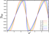
Figure 1: Schematic illustration of the GW amplitude $h_{xx}~{}(=\frac{v_{(0)}}{2c_{s0}})$ for $\beta=\frac{3}{2}$ ($\gamma=2$). We choose $v_{(0)}=A\cos kx$; $x,x^{\prime}=x-c_{s0}t$ and $t$ are in units of $1/k$ and $1/(c_{s0}k)$, respectively. Left: $h_{xx}$ in the $x,t$ plane ($A=0.05$). Right: Temporal change of initial cosine profile; greater value of $h_{xx}$ corresponds to smaller speed $v_{(0)}$, clearly visible in the frame $(x^{\prime},t)$ comoving at $c_{s0}$. Here, $t_{\rm shock}=\frac{40}{3}$.

We define the FPs as particles which move with the flow. As the FP moves $\xi$ changes; a specific value of $\xi$ gives a characteristic curve, i.e., the sound wave trajectory. The equation of motion is just $\frac{dx}{dt}=v_{(0)}$, with the initial condition $x=\xi_{i}$ at $t=0$. We find $v_{(0)}=v_{(0)}(\xi)=v(x,t)$ by solving for $\xi=\xi(x,t)$ from Eq. (17). For a sound (null) ray, $\frac{dx}{dt}=(\pm c_{s(0)}+v_{(0)})$. For $v_{(0)}>0$, $v_{(0)}<c_{s(0)}+v_{(0)}$, for $v_{(0)}<0$, $v_{(0)}>-c_{s(0)}+v_{(0)}$, we have already established in the above that $v_{(0)}<c_{s(0)}$ and $c_{s(0)}=c_{s0}+\beta v_{(0)}$. We conclude that $\forall(x,t)$ the FP lies inside an intersecting pair of null lines. To visualize the change in shape of the wave profile, due to the nonlinearity, $\beta\neq 0$, in the Riemann Eq. (16), we construct a comoving reference $(x^{\prime},t)$ frame moving at $c_{s0}$ along the positive $x$ axis, cf. the right plot in Fig. 1.

To establish the analogy, we need, as explained in the above, to realize a permanent change in the metric after the GW has passed. For simplicity, we choose to work with $v_{(0)}=f(\xi)=B$ for $0<\xi<\frac{n\pi}{2k}$; $v_{(0)}=f(\xi)=A\cos k\xi+B$ for $\frac{n\pi}{2k}\leq\xi\leq\xi_{i}$ with $n$ being a positive odd integer, $f(\xi_{i})=0$. This wave profile of $v_{(0)}$ causes a permanent change in $h_{\mu\nu}$ once the the GW has passed. We note that even if one were to consider a FP following the geodesic equation of phonons and not moving with the flow, constant $h_{\mu\nu}$ would produce no relative acceleration between two FPs. The permanent metric changes in the metric components due to the presence of such a constant part at the trailing end of the GW signal then are, up to second order in the velocity perturbation constant $B$,

$$\Delta h_{tt} = \left(-\frac{(\gamma+1)}{2}c_{s0}B+\frac{3-\gamma}{4}B^{2}\right),$$

$$\Delta h_{tx} = \left(-B-\frac{(3-\gamma)}{2}\frac{B^{2}}{c_{s0}}\right),$$

$$\Delta h_{xx} = \left(\frac{(3-\gamma)}{2}\frac{B}{c_{s0}}+\frac{(3-\gamma)(2-\gamma)}{4}\frac{B^{2}}{c_{s0}^{2}}\right).$$ (18)

Distinct from the real transverse GW, we have a longitudinal wave in the BEC medium as the acoustic analogue of a GW in our fluid-dynamical set up. Here the component $h_{xx}$ plays a similar role to that of the transverse component $h_{+}$ in a real GW. We observe here that the nonlinear part of analogue GW memory, in distinction to its Einstein-gravitational counterpart, is also nonvanishing in the (however hypothetical, because thermodynamically unstable) case when $\beta=0$ ($\gamma=-1$). This is due to the relation (15) ($v_{(0)}^{2}$ terms do not vanish for $\beta=0$) and thus reflects the underlying structure of the medium (a polytropic gas), in which the analogue GW propagates. We also note that $\beta=2$ ($\gamma=3$) is a special case. Using Eq. (15), which for $\beta=2$ yields a linear relation between density and velocity perturbations, one readily shows that $\Delta h_{xx}=0$ to any order in $B$, and that in $\Delta h_{tt}$ and $\Delta h_{tx}$ all terms higher than linear in $B$ exactly vanish.

IV Experimental setup

IV.1 Phase-imprinting memory analogues

To provide a memory-related quantity which can be experimentally accessed by a quantum-optical observer in the laboratory, we consider specifically a homogeneous cloud of ultracold atoms in a cylindrical box trap Gaunt et al. (2013) with radius $R\,(\ll\xi_{c})$ and length $L\,(\gg\xi_{c})$, see Fig. 3. We suggest to employ the phase imprinting technique, readily available in the quantum optical setup of ultracold gases Denschlag et al. (2000); Leanhardt et al. (2002), to implement a specific GW profile corresponding to the initial velocity perturbation. We create a spatial variation in the phase of the initial condensate wave function, within the source region ($S$) of length $l$, by red-detuned laser light turned on for a short duration $T$ (as short as to stay within the Raman-Nath regime of simple diffraction). The superfluid phase pattern $\Phi(x)\propto I(x)/\delta$, corresponding to the velocity pattern discussed above, where $I(x)$ is laser intensity and $\delta$ detuning from resonance, is then imprinted in $S$, where the phase profile is chosen as

$$\Phi(x) = Bx+C,\quad{\mbox{for}~{}0<x<\frac{n\pi}{2k}},$$

$$\Phi(x) = \frac{A}{k}\sin(kx)+Bx+C,{\quad\mbox{for}~{}\frac{n\pi}{2k}\leq x<l},$$ (19)

where $n$ is an odd integer. Here, we put $A,B,C\geq 0$, and the constant $C$ is chosen such that $\Phi(x)>0$ within S (red-detuning $\forall\,x\in S$), cf. 2 for an illustration of the resulting $h_{xx}$ component. We note that in the $h_{xx}$ series, using in (III) the relation (15) (with a $+$ sign), the second power term in $v$ does not appear for a BEC which has $\gamma=2$, and we have $h_{xx}={v}/{2c_{s0}}$ up to cubic order.

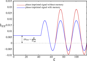
Figure 2: The initial $t=0$ metric $h_{xx}$ according to Eq. (13) in the source region, reasulting in a GW with memory [blue curve, for $B=A/2$, $A=0.025$, and $n=7$ in Eq. (IV.1)], and without memory [red curve, for which we set $\Phi(x)=0.0375\cos(0.25x)+0.01875x$ for $\frac{64\pi}{3}\leq x\leq\frac{112\pi}{3}$; and $\Phi(x)={\rm constant}$ for $0\leq x<\frac{64\pi}{3}$]. We put $k=0.25\xi_{c}^{-1}$; $B/A=1/2$, $A=0.025$ in units of $c_{s0}$, and $\xi$ is in units of the healing length $\xi_{c}$. The length of the source region is assumed to be $l=\frac{112\pi}{3}\xi_{c}$. Here, $\xi_{c}=1.8\,\mu$m (as in Ref. Muñoz de Nova et al. (2019)). For the profile with memory, this results in $l=0.21$ mm, less than the maximum allowed value of $l=0.23$ mm, which would lead to shock formation.

To simplify the calculation, we choose to work with the above nonsmooth ansatz for $\Phi$ (noting that experimentally any required smooth profile can be engineered). The thus created bipartite 1D configuration, cf. Fig. 3, produces simple waves Landau and Lifshitz (1987). At $t=0$, $v_{(0)}(\xi_{i})=v_{(0)}(l)=0\Rightarrow B<A$; this is how the constant magnitude of the profile at its edge is bounded by the amplitude in the oscillatory part in the front. Considering ${}^{87}\!$Rb as a BEC as employed in the Hawking radiation experiment of Ref. Muñoz de Nova et al. (2019), with healing length $\xi_{c}=1.8\,\mu$m (geometrically averaged between upstream and downstream regions relative to the horizon), we also have $c_{s0}=0.39$ mm/sec. We consider that the amplitude $A/c_{s0}=0.025$, and that the wavevector $k=0.25\xi_{c}^{-1}$ is of order the dominant Hawking mode in Ref. Muñoz de Nova et al. (2019). Such a value of $k$ can be achieved by phase-imprinting with an infrared laser.

We now aim at generating the memory associated to $h_{xx}$, similar to what we expect to have in the $h_{+}$ signal for a real GW in relative proportion to the highest magnitude of the oscillatory part of the GW. The maximum value of $h_{xx}$ in the oscillatory part of the phase-imprinted simple wave in Eq. (IV.1) is $\frac{(A+B)c_{s0}}{2}$, and the expression (III) yields $Bc_{s0}/2$ (for a BEC $\gamma=2$). Therefore $\frac{B}{A}=\frac{1}{n^{\prime}}$ with $n^{\prime}\geq 1$, produces a signal having a memory part $1/(1+n^{\prime})$th of the maximum value in the oscillatory part. We denote this ratio $w=1/(1+n^{\prime})$. Hence in the specific phase-imprinting example (IV.1), $w\leq 1/2,~{}\because n^{\prime}\geq 1$. For example, referring here to Fig. 1 in the review of Ref. Favata (2010), which displays a typical gravitational wave signal having memory, $w$ is there roughly $1/3$, and thus the corresponding value of $n^{\prime}$ used for phase-imprinting is about two.

In the region of observation (RO), the observers in the lab take density images by absorption imaging at discrete times. A constant density tail of the wave in the RO, as depicted in the Fig. 3 represents the memory of the signal. Eq. (15) gives this constant density shift, which is, up to order $B^{2}$,

$$\Delta\rho=\rho_{0}\left(\frac{B}{c_{s0}}+\frac{(3-\gamma)}{4}\frac{B^{2}}{c_{s0}^{2}}\right)~{}\mbox{with }B<A<c_{s0}.$$ (20)

An auxiliary condition is that discontinuities due to a shock developing have to be avoided. The mean speed of the signal equals the speed of the constant part of the wave train, i.e., $c_{s0}+\beta B$, as follows from Eq. (17). The wave train’s oscillatory part encounters a shock at $t=t_{\rm shock}=\frac{1}{\beta Ak}$ (cf. Appendix B). To avoid discontinuities, we thus design the experiment such that $\frac{l}{(c_{s0}+\beta B)}<t_{\rm shock}$. With the aforementioned parameters from Muñoz de Nova et al. (2019), $t_{\rm shock}=0.57$ sec; for $B/A=1/2$, $A=0.025$, $l<0.23$ mm. Absorption images are then taken at times $t<t_{\rm shock}$.

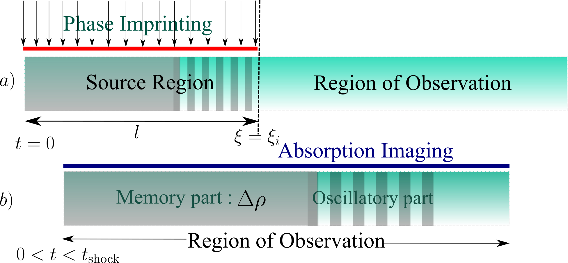
Figure 3: Observing the acoustic analogue of GW memory in a quasi-1D BEC. The grey shading represents the schematic density variation. a) The GW signal with memory is produced in the source region by phase imprinting at $t=0$, b) Zoomed-in region of observation at a time of observation less than $t_{\rm shock}$. The uniform grey shading represents constant density [increase or decrease depending on the sign of $B$ in Eq.(20)]. The memory of the signal is captured by absorption imaging when the oscillatory part is already completely residing within the region of observation.

IV.2 A proposal for simulating more realistic signals

In the case of a real GW, the transverse part of $h_{\mu\nu}$, $h_{+}$, is an observable and the memory part of it, e.g., depends on the total mass of the binary system, its reduced mass ratio, the distance between source and observer, the angle between source and direction of observation, and on the time evolution of the dominant source quadrupole moment from $t\rightarrow-\infty$ to the retarded time of detection, see for a discussion Ref. Favata (2009). The latter detection time can in principle be arbitrarily large, distinct from our analogue nonlinear acoustics model. In our setup, we have an indirect memory signal because we are not measuring permanent changes in the acoustic metric (however see below). This indirect observable is a change in density, and the signal is longitudinal. We can however in principle engineer a more realistic profile (possible by phase imprinting) having an inspiral part and a ringdown part along with a memory part (referring here again to Fig. 1 of Ref. Favata (2010)) by knowing the Fourier spectrum of the signal, where an obvious rescaling of the length scales and time scales of the real GW signal will need to be performed.

IV.3 Direct method to access metric changes

As stated in the above, measuring $\Delta\rho$ is an indirect method of observing the permanent change in the metric as expressed of Eq. 18. We now propose to access more directly the permanent change in the metric by observing the time it takes for sound rays to propagate in the presence of the analogue GW signal. Let us assume a sound ray propagating on top of the simple Riemann wave in the region of observation. From Eq. (14), the sound cone will have different opening angles in the presence of the GW which may be represented as

$$\frac{c_{s0}dt}{dx}=\frac{-\frac{h_{tx}}{c_{s0}}\pm\sqrt{\frac{h_{tx}^{2}}{c_{s0}^{2}}-(1+h_{xx})(-1+\frac{h_{tt}}{c_{s0}^{2}})}}{(-1+\frac{h_{tt}}{c_{s0}^{2}})}.$$ (21)

Putting $h_{\mu\nu}$ to zero, one verifies that $\frac{c_{s0}dt}{dx}=\pm 1$. As the sound ray passes, in the memory region we have $h_{\mu\nu}=\Delta h_{\mu\nu}$. With the values chosen in the above, $B/A=1/2$, $A=0.025$, we obtain for the sound ray going in the direction of GW propagation, $\frac{c_{s0}dt}{dx}\simeq 0.98$, and for the sound ray going opposite to the direction of the GW, $\frac{c_{s0}dt}{dx}\simeq-1.01$. Therefore, detecting the travel times of sound pulses in the eikonal approximation in the presence of the GW memory potentially yields direct access to the permanent change in the metric incurred by GWs with memory.

V Conclusion

Extending the linearized analogue gravity paradigm to nonlinear acoustics, we have demonstrated that an acoustic analogue of GW memory can be simulated in a BEC.

For clarity, we delineate and reiterate now again the primary differences to Einsteinian GW memory, also see Appendix C: (a) Our GW analogue is a longitudinal (instead of transverse) wave and lives in 1+1D; (b) it is imposed locally by a quantum optical experiment, whereas an Einsteinian GW in 3+1D contains the physical distance $r_{s}$ from source to detector; (c) The Einsteinian GW and its memory is detected by relative geodesic acceleration.

The acoustic GW memory analogue, on the other hand, offers an alternative perspective on GW memory allowing to disentangle its fundamental aspects. For GW memory and its acoustic analogue, e.g., the impact of the effective equation of state of the underlying “ether” on the memory signal can be studied. The acoustic memory analogue can potentially play a role akin to Hawking radiation analogues, which led to the clear recognition that distinct from black hole entropy, radiation is of a kinematical rather than Einstein-dynamical origin Visser (1998). Checking the “ether” dependence can for example be performed by phase-imprinting in ultracold gases waveforms akin to those of real gravitational waves, and then checking whether the memory signal response of real and acoustic GW memory displays a qualitatively similar behavior. Finally, ultracold gases lend themselves naturally to the simulation of the impact of exotic solitonic or vortical structures Denschlag et al. (2000); Leanhardt et al. (2002) in the GW train onto characteristic features of the memory signal.

Looking further ahead, we expect a significant number of novel insights gained from the inherently nonlinear dynamics of fluids for simulating curved spacetimes. Apart from the concrete example of BECs discussed in the above, this applies equally well, e.g., to shallow water or fluids of light.

VI Acknowledgments

This work has been supported by the National Research Foundation of Korea under Grants No. 2017R1A2A2A05001422 and No. 2020R1A2C2008103. It is dedicated to the memory of Renaud Parentani, and his many important and thorough contributions to analyzing classical and quantum fields in the effective curved spacetimes of fluids.

Appendix A The quasi-1D gas and general dimensionality

In a quasi-1D system along the $x$ axis, the dynamics along $y$, and $z$ axes is by definition frozen out, $v^{1}=v_{(0)}$, $v^{2}=v^{3}=0$. We may then write

$$G_{\mu\nu}({\bm{r}},t)\equiv\frac{\rho_{(0)}}{c_{s(0)}}\begin{bmatrix}-(c_{s(0)}^{2}-v_{(0)}^{2})&-v_{(0)}&0&0\\ -v_{(0)}&1&0&0\\ 0&0&1&0\\ 0&0&0&1\end{bmatrix}$$ (22)

In quasi-1D, the variables $\rho_{(0)}$ (hence $c_{s(0)}$), $v_{(0)}$ are functions of $(x,t)$. Therefore, the transverse dimensions $y$, $z$ does not play any role in the fluid dynamics. Therefore, we can construct an effective metric $\mathfrak{g}^{c}_{\mu\nu}(x,t)$:

$$\mathfrak{g}^{c}_{\mu\nu}(x,t)=\frac{\rho_{(0)}}{c_{s(0)}}\begin{bmatrix}-(c_{s(0)}^{2}-v_{(0)}^{2})&-{v_{(0)}}\\ -{v_{(0)}}&1\end{bmatrix},$$ (23)

where $\mathfrak{g}^{c}_{xx}=G_{yy}=G_{zz}$. In quasi-1D, one can indeed work with $G_{\mu\nu}$, we however choose to work with $\mathfrak{g}^{c}_{\mu\nu}(x,t)$ for convenience.

In the main text, we consider this quasi-1D set up, embedded in 3D spatial dimensions. The acoustic metric gets reduced to $1+1$D from $3+1$D due to the circular (trapping) symmetry. In this section, we show that the whole analysis can be performed starting from $d+1$D embedding dimensions for general positive integer $d\geq 2$. We work with the conformal factor in $d+1$D Barceló et al. (2011). Indicating the metric with inclusion of the conformal factor by the superscript $c$, and where we assume already that transverse dimensions are frozen out, we have

$$\mathfrak{g}^{c}_{\mu\nu}(x,t)=\left(\frac{\rho_{(0)}}{c_{s(0)}}\right)^{\frac{2}{d-1}}\begin{bmatrix}-(c_{s(0)}^{2}-v_{(0)}^{2})&-v_{(0)}\\ -v_{(0)}&1\end{bmatrix}.$$ (24)

The conformal factor, $\left(\frac{\rho_{(0)}}{c_{s(0)}}\right)^{\frac{2}{d-1}}=\left(\frac{\rho_{0}}{c_{s0}}\right)^{\frac{2}{d-1}}\left(1+\frac{\delta\rho}{\rho_{0}}\right)^{\frac{3-\gamma}{d-1}}$ by using a barotropic equation of state. The nonzero constant $\left(\frac{\rho_{0}}{c_{s0}}\right)^{\frac{2}{d-1}}$ factor can be absorbed into a redefined metric. We find

$$\mathfrak{g}_{\mu\nu}(x,t)=g_{\mu\nu}+h_{\mu\nu}(x,t),$$ (25)

where the background metric is

$$g_{\mu\nu}\coloneqq\begin{bmatrix}-c_{s0}^{2}&0\\ 0&1\end{bmatrix},$$ (26)

and the perturbation metric $h_{\mu\nu}(x,t)$ is, considering terms up to second order,

$$h_{tt}=-c_{s0}^{2}\left\{\left(\frac{\gamma(d-2)-d+4}{d-1}\right)\frac{\delta\rho}{\rho_{0}}+\left(\frac{(\gamma(d-2)-d+4)(\gamma(d-2)-2d+5)}{2(d-1)^{2}}\right)\left(\frac{\delta\rho}{\rho_{0}}\right)^{2}\right\}+v^{2},$$ (27)

$$h_{tx}=h_{xt}=-v\left(1+\frac{(3-\gamma)}{(d-1)}\frac{\delta\rho}{\rho_{0}}\right),\qquad h_{xx}=\left(\frac{3-\gamma}{d-1}\right)\frac{\delta\rho}{\rho_{0}}+\frac{(3-\gamma)(4-\gamma-d)}{2(d-1)^{2}}\left(\frac{\delta\rho}{\rho_{0}}\right)^{2}.$$ (28)

Note that the perturbed fluid velocities $v$ and $v_{(0)}$ are identical because we start with a static background.

Appendix B Shock waves

We consider for simplicity an initially monochromatic wave travelling along the $x$ axis, which has $v_{(0)}=A\cos k\xi$. Hence, we find from the Eq. (17) in the main text

$$x=\left(c_{s0}+\beta A\cos k\xi\right)t+\xi.$$ (29)

Therefore, we also find, by using (29),

$$\partial_{t}v_{(0)}=-Ak\sin(k\xi)\partial_{t}\xi=-Ak\frac{(c_{s0}+A\cos k\xi)}{\left(\beta Akt\sin k\xi-1\right)}\sin k\xi,$$

$$\partial_{x}v_{(0)}=-Ak\sin(k\xi)\partial_{x}\xi=\frac{Ak\sin k\xi}{\beta Akt\sin k\xi-1}.$$ (30)

Using the above two equations, one can check that the Riemann equation (16) is satisfied. One can also see that at $t=t_{\rm shock}$, $\partial_{t}v_{(0)}$ and $\partial_{x}v_{(0)}$, become infinity. Different $\xi$ values correspond to different $t_{\rm shock}$, and the minimum value of $t_{\rm shock}$ is given by

$$t_{\rm shock}=\frac{1}{\beta Ak},$$ (31)

which is inversely proportional to the amplitude of velocity perturbation, $A$. Evidently, the expression Eq. (31), remains unchanged if we add a constatnt to $v_{(0)}$, i.e., $v_{(0)}=A\cos k\xi+B$. For $t>t_{\rm shock}$, the density and velocity of the medium becomes multivalued, i.e., at a single coordinate $(x,t)$, more than one solution in $v_{(0)}$ and $\rho_{(0)}$ exists. This singular situation for $t>t_{\rm shock}$ is handled by introducing discontinuities in density and velocity, as discussed in Landau and Lifshitz (1987); Enflo and Hedberg (2006). Discontinuous density and velocity solutions are generally called shock solutions.

Appendix C GW memory in general relativity vs analogue memory

C.1 Memory effect in general relativity

Owing to general covariance, the movement of a single test particle by GW can be nullified to first order in the (traceless-transverse gauge) perturbation $h_{\mu\nu}^{TT}$ by a proper choice of coordinates Carroll (2019), and relative displacements of at least two test particles have to be employed to ascertain the impact of a GW Weinberg (1972); Carroll (2019). To measure the motion of a single test particle, we would then need to compare its displacement to neighboring objects (in some definite reference frame) which are also moving with the GW.

The memory effect is characterized by the permanent change in separation between two freely falling particles (ideal detector) after a GW train has passed. The vectorial separation between two freely falling particles initially at rest relative two each other separated by a distance $l^{k}$, changes due to the GW field. The vectorial change $\delta l_{j}$ is given by (as derived from the equation of geodesic deviation) Carroll (2019)

$$\delta l_{j}=\frac{1}{2}h_{jk}^{TT}l^{k}.$$ (32)

After a GW causing no memory has passed, $\delta l_{j}$ becomes zero, and the test particles come back to their original positions, which is not the case for a GW presenting memory. We note in this regard that the precise nature of GW memory, as originally proposed in Zel’dovich and Polnarev (1974), has been debated. Arguments have been put forward that after the (plane) GW wave train has passed, two given freely falling test particles do not come to rest again, as stated by Zel’dovich and Polnarev (1974), but retain a finite velocity relative to each other Grishchuk and Polnarev (1989); Bondi and Pirani (1989); Zhang et al. (2017).

C.2 Memory effect in the analogue model

In analogue models, general (coordinate) covariance is absent. In other words, for our analogue, the observers in the lab are not affected by the GW which is a sound wave propagating in the BEC medium. In the analogue models based on the description of fluid motion in Newtonian framework, the notion of time and space is absolute Newton (1687), which is simply reflected in the preferred frame of the (Newtonian) lab in which the experimentalist carries out his or her work.

To build our analogy, we defined in the main text fiducial test particles which move with the flow. We note here that one can imagine to define internal observers in the spirit of Ref. Barceló and Jannes (2008). In the latter reference, the authors postulate the existence of internal observers as observers living in a world of phonons, which can perform Michelson-Morley type interferometry with them. This gedankenexperiment then gives a zero fringe-shift (null) result explained by the Lorentz-FitzGerald contraction in such an internal phononic world. However, the internal observer picture, in our context, comes with an inherent difficulty. For nonlinear sound, signal propagation depends on the amplitude of perturbations [cf. Eq. (16)) One would therefore be posed with the formidable task to construct, for obtaining a null result, an internal phonon interferometer which has nonlinear Lorentz-FitzGerald contraction for different signal amplitudes. On the other hand, even if general covariance is lost in the case of nonlinear sound, we can still define an internal observer in the phononic world, which is having access to the acoustic metric.

References

- Abbott et al. (2016) B. P. Abbott et al. (LIGO Scientific Collaboration and Virgo Collaboration), “Observation of Gravitational Waves from a Binary Black Hole Merger,” Phys. Rev. Lett. 116, 061102 (2016).
- Zel’dovich and Polnarev (1974) Ya. B. Zel’dovich and A. G. Polnarev, “Radiation of gravitational waves by a cluster of superdense stars,” Sov. Astron. 18, 17 (1974).
- Braginskiǐ and Grishchuk (1985) V. B. Braginskiǐ and L. P. Grishchuk, “Kinematic Resonance and Memory Effect in Free Mass Gravitational Antennas,” Sov. Phys. JETP 62, 427–430 (1985).
- Braginsky and Thorne (1987) Vladimir B. Braginsky and Kip S. Thorne, “Gravitational-wave bursts with memory and experimental prospects,” Nature 327, 123–125 (1987).
- Christodoulou (1991) Demetrios Christodoulou, “Nonlinear nature of gravitation and gravitational-wave experiments,” Phys. Rev. Lett. 67, 1486–1489 (1991).
- Thorne (1992) Kip S. Thorne, “Gravitational-wave bursts with memory: The Christodoulou effect,” Phys. Rev. D 45, 520–524 (1992).
- Favata (2010) Marc Favata, “The gravitational-wave memory effect,” Classical and Quantum Gravity 27, 084036 (2010).
- Johnson et al. (2019) Aaron D. Johnson, Shasvath J. Kapadia, Andrew Osborne, Alex Hixon, and Daniel Kennefick, “Prospects of detecting the nonlinear gravitational wave memory,” Phys. Rev. D 99, 044045 (2019).
- Boersma et al. (2020) Oliver M. Boersma, David A. Nichols, and Patricia Schmidt, “Forecasts for detecting the gravitational-wave memory effect with Advanced LIGO and Virgo,” Phys. Rev. D 101, 083026 (2020).
- Wiseman and Will (1991) Alan G. Wiseman and Clifford M. Will, “Christodoulou’s nonlinear gravitational-wave memory: Evaluation in the quadrupole approximation,” Phys. Rev. D 44, R2945–R2949 (1991).
- Barceló et al. (2011) Carlos Barceló, Stefano Liberati, and Matt Visser, “Analogue Gravity,” Living Reviews in Relativity 14, 3 (2011).
- Volovik (2009) G.E. Volovik, The Universe in a Helium Droplet, International Series of Monographs on Physics (OUP Oxford, 2009).
- Unruh (1981) W. G. Unruh, “Experimental Black-Hole Evaporation?” Phys. Rev. Lett. 46, 1351–1353 (1981).
- Schützhold and Unruh (2002) Ralf Schützhold and William G. Unruh, “Gravity wave analogues of black holes,” Phys. Rev. D 66, 044019 (2002).
- Weinfurtner et al. (2011) Silke Weinfurtner, Edmund W. Tedford, Matthew C. J. Penrice, William G. Unruh, and Gregory A. Lawrence, “Measurement of Stimulated Hawking Emission in an Analogue System,” Phys. Rev. Lett. 106, 021302 (2011).
- Euvé et al. (2016) L.-P. Euvé, F. Michel, R. Parentani, T. G. Philbin, and G. Rousseaux, “Observation of Noise Correlated by the Hawking Effect in a Water Tank,” Phys. Rev. Lett. 117, 121301 (2016).
- Euvé et al. (2020) Léo-Paul Euvé, Scott Robertson, Nicolas James, Alessandro Fabbri, and Germain Rousseaux, “Scattering of Co-Current Surface Waves on an Analogue Black Hole,” Phys. Rev. Lett. 124, 141101 (2020).
- Marino (2008) Francesco Marino, “Acoustic black holes in a two-dimensional “photon fluid”,” Phys. Rev. A 78, 063804 (2008).
- Nguyen et al. (2015) H. S. Nguyen, D. Gerace, I. Carusotto, D. Sanvitto, E. Galopin, A. Lemaître, I. Sagnes, J. Bloch, and A. Amo, “Acoustic Black Hole in a Stationary Hydrodynamic Flow of Microcavity Polaritons,” Phys. Rev. Lett. 114, 036402 (2015).
- Garay et al. (2000) L. J. Garay, J. R. Anglin, J. I. Cirac, and P. Zoller, “Sonic Analog of Gravitational Black Holes in Bose-Einstein Condensates,” Phys. Rev. Lett. 85, 4643–4647 (2000).
- Carusotto et al. (2008) Iacopo Carusotto, Serena Fagnocchi, Alessio Recati, Roberto Balbinot, and Alessandro Fabbri, “Numerical observation of Hawking radiation from acoustic black holes in atomic Bose–Einstein condensates,” New Journal of Physics 10, 103001 (2008).
- Macher and Parentani (2009) Jean Macher and Renaud Parentani, “Black-hole radiation in Bose-Einstein condensates,” Phys. Rev. A 80, 043601 (2009).
- Gerace and Carusotto (2012) Dario Gerace and Iacopo Carusotto, “Analog Hawking radiation from an acoustic black hole in a flowing polariton superfluid,” Phys. Rev. B 86, 144505 (2012).
- Steinhauer (2016) J. Steinhauer, “Observation of quantum Hawking radiation and its entanglement in an analogue black hole,” Nat. Phys. 12, 959–965 (2016).
- Muñoz de Nova et al. (2019) Juan Ramón Muñoz de Nova, Katrine Golubkov, Victor I. Kolobov, and Jeff Steinhauer, “Observation of thermal Hawking radiation and its temperature in an analogue black hole,” Nature 569, 688–691 (2019).
- Fischer and Schützhold (2004) U. R. Fischer and R. Schützhold, “Quantum simulation of cosmic inflation in two-component Bose-Einstein condensates,” Phys. Rev. A 70, 063615 (2004).
- Chä and Fischer (2017) Seok-Yeong Chä and Uwe R. Fischer, “Probing the Scale Invariance of the Inflationary Power Spectrum in Expanding Quasi-Two-Dimensional Dipolar Condensates,” Phys. Rev. Lett. 118, 130404 (2017).
- Eckel et al. (2018) S. Eckel, A. Kumar, T. Jacobson, I. B. Spielman, and G. K. Campbell, “A Rapidly Expanding Bose-Einstein Condensate: An Expanding Universe in the Lab,” Phys. Rev. X 8, 021021 (2018).
- Barceló et al. (2003) C. Barceló, S. Liberati, and M. Visser, “Probing semiclassical analog gravity in Bose-Einstein condensates with widely tunable interactions,” Phys. Rev. A 68, 053613 (2003).
- Fedichev and Fischer (2004) P. O. Fedichev and U. R. Fischer, ““Cosmological” quasiparticle production in harmonically trapped superfluid gases,” Phys. Rev. A 69, 033602 (2004).
- Busch et al. (2014) Xavier Busch, Iacopo Carusotto, and Renaud Parentani, “Spectrum and entanglement of phonons in quantum fluids of light,” Phys. Rev. A 89, 043819 (2014).
- Robertson et al. (2017) Scott Robertson, Florent Michel, and Renaud Parentani, “Assessing degrees of entanglement of phonon states in atomic Bose gases through the measurement of commuting observables,” Phys. Rev. D 96, 045012 (2017).
- Tian et al. (2018) Zehua Tian, Seok-Yeong Chä, and Uwe R. Fischer, “Roton entanglement in quenched dipolar Bose-Einstein condensates,” Phys. Rev. A 97, 063611 (2018).
- Fedichev and Fischer (2003) P. O. Fedichev and U. R. Fischer, “Gibbons-Hawking Effect in the Sonic de Sitter Space-Time of an Expanding Bose-Einstein-Condensed Gas,” Phys. Rev. Lett. 91, 240407 (2003).
- Retzker et al. (2008) A. Retzker, J. I. Cirac, M. B. Plenio, and B. Reznik, “Methods for Detecting Acceleration Radiation in a Bose-Einstein Condensate,” Phys. Rev. Lett. 101, 110402 (2008).
- Kosior et al. (2018) Arkadiusz Kosior, Maciej Lewenstein, and Alessio Celi, “Unruh effect for interacting particles with ultracold atoms,” SciPost Phys. 5, 61 (2018).
- Gooding et al. (2020) Cisco Gooding, Steffen Biermann, Sebastian Erne, Jorma Louko, William G. Unruh, Jörg Schmiedmayer, and Silke Weinfurtner, “Interferometric Unruh Detectors for Bose-Einstein Condensates,” Phys. Rev. Lett. 125, 213603 (2020).
- Corley and Jacobson (1999) Steven Corley and Ted Jacobson, “Black hole lasers,” Phys. Rev. D 59, 124011 (1999).
- Finazzi and Parentani (2010) S. Finazzi and R. Parentani, “Black hole lasers in Bose–Einstein condensates,” New Journal of Physics 12, 095015 (2010).
- Basak and Majumdar (2003) Soumen Basak and Parthasarathi Majumdar, “‘Superresonance’ from a rotating acoustic black hole,” Classical and Quantum Gravity 20, 3907–3913 (2003).
- Torres et al. (2017) Theo Torres, Sam Patrick, Antonin Coutant, Maurício Richartz, Edmund W. Tedford, and Silke Weinfurtner, “Rotational superradiant scattering in a vortex flow,” Nature Physics 13, 833–836 (2017).
- Prain et al. (2019) Angus Prain, Calum Maitland, Daniele Faccio, and Francesco Marino, “Superradiant scattering in fluids of light,” Phys. Rev. D 100, 024037 (2019).
- Berti et al. (2004) Emanuele Berti, Vitor Cardoso, and José P. S. Lemos, “Quasinormal modes and classical wave propagation in analogue black holes,” Phys. Rev. D 70, 124006 (2004).
- Torres et al. (2020) Theo Torres, Sam Patrick, Maurício Richartz, and Silke Weinfurtner, “Quasinormal mode oscillations in an analogue black hole experiment,” Phys. Rev. Lett. 125, 011301 (2020).
- Hartley et al. (2018) Daniel Hartley, Tupac Bravo, Dennis Rätzel, Richard Howl, and Ivette Fuentes, “Analogue simulation of gravitational waves in a -dimensional Bose-Einstein condensate,” Phys. Rev. D 98, 025011 (2018).
- Datta (2018) Satadal Datta, “Acoustic analog of gravitational wave,” Phys. Rev. D 98, 064049 (2018).
- Barceló et al. (2001) Carlos Barceló, Stefano Liberati, and Matt Visser, “Analogue gravity from field theory normal modes?” Classical and Quantum Gravity 18, 3595–3610 (2001).
- Fischer and Visser (2003) Uwe R. Fischer and Matt Visser, “On the space-time curvature experienced by quasiparticle excitations in the Painlevé–Gullstrand effective geometry,” Annals of Physics 304, 22–39 (2003).
- Bieri and Garfinkle (2013) Lydia Bieri and David Garfinkle, “An electromagnetic analogue of gravitational wave memory,” Classical and Quantum Gravity 30, 195009 (2013).
- Pate et al. (2017) Monica Pate, Ana-Maria Raclariu, and Andrew Strominger, “Color Memory: A Yang-Mills Analog of Gravitational Wave Memory,” Phys. Rev. Lett. 119, 261602 (2017).
- Pitaevskiǐ and Stringari (2003) L. P. Pitaevskiǐ and S. Stringari, Bose-Einstein Condensation, International Series of Monographs on Physics (Clarendon Press, Oxford, 2003).
- Gaunt et al. (2013) Alexander L. Gaunt, Tobias F. Schmidutz, Igor Gotlibovych, Robert P. Smith, and Zoran Hadzibabic, “Bose-Einstein Condensation of Atoms in a Uniform Potential,” Phys. Rev. Lett. 110, 200406 (2013).
- Görlitz et al. (2001) A. Görlitz, J. M. Vogels, A. E. Leanhardt, C. Raman, T. L. Gustavson, J. R. Abo-Shaeer, A. P. Chikkatur, S. Gupta, S. Inouye, T. Rosenband, and W. Ketterle, “Realization of Bose-Einstein Condensates in Lower Dimensions,” Phys. Rev. Lett. 87, 130402 (2001).
- Datta and Fischer (2021) Satadal Datta and Uwe R. Fischer, “Analogue gravitational field from nonlinear fluid dynamics,” (2021), arXiv:2110.11083 [gr-qc] .
- Riemann (1860) Bernhard Riemann, “Ueber die Fortpflanzung ebener Luftwellen von endlicher Schwingungsweite,” Abhandlungen der Königlichen Gesellschaft der Wissenschaften in Göttingen 8, 43–66 (1860).
- Nemirovskiǐ (1990) S. K. Nemirovskiǐ, “Nonlinear acoustics of superfluid helium,” Soviet Physics Uspekhi 33, 429–452 (1990).
- Enflo and Hedberg (2006) Bengt O. Enflo and Claes M. Hedberg, Theory of nonlinear acoustics in fluids, Vol. 67 (Springer Science & Business Media, 2006).
- Söoderholm (2001) Lars H. Söoderholm, “A Higher Order Acoustic Equation for the Slightly Viscous Case,” Acta Acustica united with Acustica 87, 29–33 (2001).
- Hamilton et al. (1998) Mark F. Hamilton, David T. Blackstock, et al., Nonlinear acoustics, Vol. 237 (Academic Press, San Diego, 1998).
- Kuznetsov (1971) V. P. Kuznetsov, “Equations of nonlinear acoustics,” Sov. Phys. Acoust. 16, 467–470 (1971).
- Landau and Lifshitz (1987) L. D. Landau and E. M. Lifshitz, Fluid Mechanics, Second Edition: Volume 6 (Course of Theoretical Physics), 2nd ed. (Butterworth-Heinemann, 1987).
- Harumi (2019) Hattori Harumi, Partial differential equations: methods, applications and theories (World Scientific, 2019).
- Marino et al. (2016) F. Marino, C. Maitland, D. Vocke, A. Ortolan, and D. Faccio, “Emergent geometries and nonlinear-wave dynamics in photon fluids,” Scientific Reports 6, 23282 (2016).
- Kamchatnov et al. (2004) A. M. Kamchatnov, A. Gammal, and R. A. Kraenkel, “Dissipationless shock waves in Bose-Einstein condensates with repulsive interaction between atoms,” Phys. Rev. A 69, 063605 (2004).
- Meppelink et al. (2009) R. Meppelink, S. B. Koller, J. M. Vogels, P. van der Straten, E. D. van Ooijen, N. R. Heckenberg, H. Rubinsztein-Dunlop, S. A. Haine, and M. J. Davis, “Observation of shock waves in a large Bose-Einstein condensate,” Phys. Rev. A 80, 043606 (2009).
- Damski (2004) Bogdan Damski, “Formation of shock waves in a bose-einstein condensate,” Phys. Rev. A 69, 043610 (2004).
- Carroll (2019) Sean M Carroll, Spacetime and geometry (Cambridge University Press, 2019).
- Denschlag et al. (2000) J. Denschlag, J. E. Simsarian, D. L. Feder, Charles W. Clark, L. A. Collins, J. Cubizolles, L. Deng, E. W. Hagley, K. Helmerson, W. P. Reinhardt, S. L. Rolston, B. I. Schneider, and W. D. Phillips, “Generating Solitons by Phase Engineering of a Bose-Einstein Condensate,” Science 287, 97–101 (2000).
- Leanhardt et al. (2002) A. E. Leanhardt, A. Görlitz, A. P. Chikkatur, D. Kielpinski, Y. Shin, D. E. Pritchard, and W. Ketterle, “Imprinting Vortices in a Bose-Einstein Condensate using Topological Phases,” Phys. Rev. Lett. 89, 190403 (2002).
- Favata (2009) Marc Favata, “Nonlinear gravitational-wave memory from binary black hole mergers,” Astrophys. J. 696, L159–L162 (2009).
- Visser (1998) Matt Visser, “Hawking Radiation without Black Hole Entropy,” Phys. Rev. Lett. 80, 3436–3439 (1998).
- Weinberg (1972) Steven Weinberg, Gravitation and cosmology: principles and applications of the general theory of relativity (Wiley, 1972).
- Grishchuk and Polnarev (1989) L. P. Grishchuk and A. G. Polnarev, “Gravitational wave pulses with “velocity coded memory”,” Sov. Phys. JETP 69, 653–657 (1989).
- Bondi and Pirani (1989) Hermann Bondi and F. A. E. Pirani, “Gravitational waves in general relativity - XIII. Caustic property of plane waves,” Proceedings of the Royal Society of London. A. Mathematical and Physical Sciences 421, 395–410 (1989).
- Zhang et al. (2017) P. M. Zhang, C. Duval, G. W. Gibbons, and P. A. Horvathy, “The memory effect for plane gravitational waves,” Physics Letters B 772, 743–746 (2017).
- Newton (1687) Isaac Newton, Philosophiae naturalis principia mathematica (Londini, Jussu Societatis Regiae ac Typis Josephi Streater. Prostat apud plures Bibliopolas, 1687).
- Barceló and Jannes (2008) Carlos Barceló and Gil Jannes, “A Real Lorentz-FitzGerald Contraction,” Foundations of Physics 38, 191–199 (2008).