A Smale-Barden manifold admitting K-contact but not Sasakian structure

Abstract.

We give the first example of a simply connected compact $5$-manifold (Smale-Barden manifold) which admits a K-contact structure but does not admit any Sasakian structure, settling a long standing question of Boyer and Galicki.

1. Introduction

In geometry, a central question is to determine when a given manifold admits a specific geometric structure. Complex geometry provides numerous examples of compact manifolds with rich topology, and there is a number of topological properties that are satisfied by Kähler manifolds [1, 15]. If we forget about the integrability of the complex structure, then we are dealing with symplectic manifolds. There has been enormous interest in the construction of (compact) symplectic manifolds that do not admit Kähler structures, and in determining its topological properties [27]. The fundamental group is one of the more direct invariants that constrain the topology of Kähler manifolds [15], whereas any finitely presented group can be the fundamental group of a compact symplectic manifold [18]. For this reason, the problem becomes more relevant if we ask for simply connected compact manifolds. On the other hand, the difficulties increase as we look for manifolds of the lowest possible dimension. For instance, the lowest dimension for a compact simply connected manifold admitting a symplectic but not a Kähler structure and having non-formal rational homotopy type is $8$. Such an example was first provided by Fernández and the author in [16]. Also, a compact simply connected manifold admitting both a symplectic and a complex structure but not a Kähler structure can only happen in dimensions higher than $6$. The first example of such instance in the lowest dimension $6$ is given by Bazzoni, Fernández and the author in [4].

A symplectic manifold always admits an almost-Kähler structure (which is a metric structure), so the topological question above can be rephrased as to finding manifolds which admit almost-Kähler but no Kähler structures. In odd dimensions, the analogues of Kähler and almost-Kähler manifolds are Sasakian and K-contact manifolds, respectively (and the analogue of symplectic manifold is contact manifold). These are metric structures which are endowed with a one-dimensional foliation and a transversal structure which is Kähler or almost-Kähler, respectively (Section 2.2 for precise definitions). Sasakian geometry has become an important and active subject since the treatise of Boyer and Galicki [7], and there is much interest on constructing K-contact manifolds which do not admit Sasakian structures. As mentioned in [7, Charpter 10], now there is a gap between contact and K-contact, and the problem of finding a manifold admitting a contact but not Sasakian structure is easily solved. However, finding manifolds which admit a K-contact but not a Sasakian structure is harder.

The parity of $b_{1}$ was used to produce the first examples of K-contact manifolds with no Sasakian structure [7, example 7.4.16]. More refined tools are needed in the case of even Betti numbers. The cohomology algebra of a Sasakian manifold satisfies a hard Lefschetz property [10], and using it examples of K-contact non-Sasakian manifolds are produced in [11] in dimensions $5$ and $7$. These examples are nilmanifolds with even Betti numbers, so in particular they are not simply connected. The fundamental group can also be used to construct K-contact non-Sasakian manifolds [13]. Also it has been used to provide an example of a solvmanifold of dimension $5$ which satisfies the hard Lefschetz property and which is K-contact and not Sasakian [12].

When one moves to the case of simply connected manifolds, K-contact non-Sasakian examples of any dimension $\geq 9$ were constructed in [19] using the evenness of the third Betti number of a compact Sasakian manifold. Alternatively, using the hard Lefschetz property for Sasakian manifolds there are examples [22] of simply connected K-contact non-Sasakian manifolds of any dimension $\geq 9$. In [6] the rational homotopy type is used to construct examples of simply connected K-contact non-Sasakian manifolds in dimensions $\geq 17$. In dimension $7$ there are examples in [26] of simply connected K-contact non-Sasakian manifolds. However, Massey products are not suitable for the analysis of lower dimensional manifolds. The problem of the existence of simply connected K-contact non-Sasakian compact manifolds is still open in dimension $5$, despite numerous attempts.

Open Problem 10.2.1 in [7]: Do there exist Smale-Barden manifolds which carry K-contact but do not carry Sasakian structures?

A simply connected compact $5$-manifold is called a Smale-Barden manifold. These manifolds are classified [2, 30] by $H_{2}(M,\mathbb{Z})$ and the second Stiefel-Whitney class (see Section 2.1). This makes sensible to pose classification problems of manifolds admiting diverse geometric structures in the class of Smale-Barden manifolds.

A Sasakian manifold $M$ always admits a quasi-regular Sasakian structure. This gives $M$ the structure of a Seifert bundle over a cyclic Kähler orbifold $X$ (see Section 2.3). In the case of a $5$-manifold, $X$ is a singular complex surface with cyclic quotient singularities. The Sasakian structure is semi-regular if the isotropy locus is only formed by codimension $2$ submanifolds, that is if $X$ is a smooth complex surface and the isotropy consists of smooth complex curves (maybe intersecting). A similar statement holds for K-contact manifolds, where the base is now an almost-Kähler orbifold (that is, symplectic with a compatible almost complex structure, which always exists) with cyclic singularities, and the isotropy locus is formed by symplectic surfaces.

In [20] Kollár determines the topology of simply connected $5$-manifolds which are Seifert bundles over semi-regular $4$-orbifolds. The torsion in $H_{2}(M,\mathbb{Z})$ is determined by the genera and isotropy coefficients of the isotropy surfaces. He uses this to produce simply connected $5$-manifolds which are Seifert bundles (that is, they admit a fixed point free circle action) but which do not admit a Sasakian structure. If the structure is semi-regular, the isotropy surfaces must satisfy the adjunction equality, so an example violating it will produce such example. In general, a Kähler orbifold can have isolated singularities which cause serious difficulties, since the classification of singular complex surfaces is far more complicated than that of smooth complex surfaces. Kollár uses the case $b_{2}(X)=1$, where there is a bound on the number of singular points, and taking enough curves for the isotropy locus ensures that some of them satisfy the adjunction equality.

To produce K-contact Smale-Barden manifolds, one needs to construct symplectic $4$-manifolds (or $4$-orbifolds with cyclic quotient singularities) with symplectic surfaces of given genus inside. If the isotropy coefficients are not coprime, these surfaces are forced to be disjoint (and linearly independent in homology). Therefore there is a bound on the number $k$ of surfaces in the isotropy locus, $k\leq b_{2}(X)$. The genus of the isotropy surfaces, the isotropy coefficients, and whether they are disjoint, are translated to the homology group $H_{2}(M,\mathbb{Z})$ of the $5$-manifold $M$. This is used in [25] to produce a homology Smale-Barden manifold (that is, a $5$-manifold $M$ with $H_{1}(M,\mathbb{Z})=0$ instead of simply connected) which admits a semi-regular K-contact but not a semi-regular Sasakian structure. For this, we construct a simply connected symplectic $4$-manifold $X$ with $k$ disjoint symplectic surfaces of positive genus where $k=b_{2}(X)$, and linearly independent in homology. To prove that this is not semi-regular Sasakian, we have to check that there is no complex surface $Y$ with $b_{1}(Y)=0$, and $k$ disjoint complex curves of positive genus where $k=b_{2}(Y)>1$, and linearly independent in homology, at least for the case where the genera match our symplectic example. The existence of so many disjoint complex curves of positive genus and generating the rational homology is certainly a rare phenomenon and we conjecture that it does never happen. Unfortunately, as the example in [9, Section 3] shows, this can happen for singular complex manifolds with cyclic singularities. For this reason, we do not know whether the example in [25] can admit a quasi-regular Sasakian structure.

Later, in [8] we extend the ideas of [25] to produce the first example of simply connected $5$-manifold which admits a semi-regular K-contact structure but not a semi-regular Sasakian structure. Again we have not been able to remove the semi-regularity assumption. The purpose of this paper is to completely settle the question in [7, Open Problem 10.2.1].

Theorem 1.

There exists a Smale-Barden manifold $M$ which admits a K-contact structure but does not admit a Sasakian structure.

More precisely, a manifold $M$ in Theorem 1 can be explicitly given as follows. There is some $N>0$ large enough, and distinct primes $p_{nm}$ with $p_{nm}>\max(3,n,m)$, $1\leq n,m\leq N$, so that $M$ is the Smale-Barden manifold characterized by the fact $M$ is spin and its homology is

$$H_{2}(M,\mathbb{Z})=\mathbb{Z}^{2}\oplus\bigoplus_{n,m=1}^{N}\left(\mathbb{Z}^{18n^{2}+2}_{p_{nm}}\oplus\mathbb{Z}^{18m^{2}+2}_{p_{nm}^{2}}\oplus\mathbb{Z}^{20}_{p_{nm}^{3}}\right).$$

Let us describe the philosophy behind the construction in Theorem 1, although the technical details, which will be carried out in the following sections, get quite involved. As we said before, for our Seifert bundles $M\to X$ we can keep track of the genera and the disjointness of the isotropy surfaces. With this we try to push the construction to record also the value of $b^{+}_{2}(X)$. We note that when $Y$ is a complex surface with $k=b_{2}(Y)$ complex curves spanning $H_{2}(Y,\mathbb{Q})$, then $b^{+}_{2}(Y)=1$, whereas the same property does not necessarily hold for symplectic $4$-manifolds. If $X$ is symplectic and $b^{+}_{2}(X)>1$, then when we have $k=b_{2}(X)$ disjoint symplectic surfaces, we can take positive multiples of those with positive self-intersection. This gives $N$ families of $k=b_{2}(X)$ disjoint symplectic surfaces, which can be used as isotropy locus, for any $N\gg 0$ as large as we want.

The proof that the resulting $5$-manifold $M$ does not admit a Sasakian structure now requires to check that there is no singular complex surface $Y$ with cyclic singularities with a large number of families, each consisting of $k=b_{2}(Y)$ disjoint complex curves. First we need to bound the number of singular points (universally, i.e. independently of $Y$) as it was done in [20] for the easy case $b_{2}(Y)=1$. This serves to bound geometric quantities, like the Euler characteristic, $K^{2}$, or the self-intersection of negative curves. For orbifolds, the intersection and self-intersection numbers and $K^{2}$ can be rational (instead of just integers), so it is necessary to bound the denominators (independently of $Y$).

As the number of singular points in bounded, we have that most of the families of disjoint complex curves avoid the singular points. However, now the genera of the curves have increased (the arguments of [8, 25] deal with cases of low genus curves, so they are not helpful now). In the families of disjoint complex curves, it cannot happen that the curves are multiples of $k$ fixed curves (incidentally, note that this was the way in which the symplectic example $X$ is produced), because that would imply that $b^{+}_{2}(Y)>1$, and this does not hold for an algebraic surface. This forces to have from the initial $N$ families of $k$ disjoint complex curves (these are orthogonal bases of $H_{2}(Y,\mathbb{Q})$), many of them whose elements are not proportional to each other (what we call proj-equivalent bases). The final step is to prove the impossibility of this situation, by writing $K^{2}$ with respect to each of the orthogonal basis, and use the bounds on the denominators of the rational numbers. We get a collection of diophantine equalities, and choosing $N$ large enough, these become incompatible.

Acknowledgements

I am grateful to Javier Fernández de Bobadilla, Marco Castrillón, Antonio Viruel and Maribel González-Vasco for encouragement. Also thanks to Matthias Schütt and Alex Tralle for very useful conversations, and to Sergio Negrete for help with designing a program to find elliptic surfaces for Section 3. Special thanks to Juan Rojo for carefully reading the manuscript and finding a mistake in a previous version, and to Ángel González-Prieto for help with drawing the pictures. Finally, I am grateful to the referees for very helpful comments that have improved the exposition, and for the kind words of praise.

2. Basic notions

2.1. Smale-Barden manifolds

A $5$-dimensional simply connected manifold is called a Smale-Barden manifold. These manifolds are classified by their second homology group over $\mathbb{Z}$ and the Barden invariant [2, 30]. In more detail, let $M$ be a compact smooth simply connected $5$-manifold and write $H_{2}(M,\mathbb{Z})$ as a direct sum of cyclic groups of prime power order

$$H_{2}(M,\mathbb{Z})=\mathbb{Z}^{k}\oplus\left(\mathop{\oplus}\limits_{p,i}\mathbb{Z}_{p^{i}}^{c(p^{i})}\right),$$ (1)

where $k=b_{2}(M)$. The equality (1) is actually an isomorphism as abelian groups. We can arrange so that the second Stiefel-Whitney class map

$$w_{2}:H_{2}(M,\mathbb{Z})\rightarrow\mathbb{Z}_{2}$$

is zero on all but one summand (or zero on all if $w_{2}=0$). For that, take an element on which it is not zero, and complete to a generating system with elements in the kernel. If $w_{2}$ is non-zero on $\mathbb{Z}_{2^{j}}$, we set $i(M)=j$; if $w_{2}$ is non-zero on a summand $\mathbb{Z}$, we set $i(M)=\infty$; if $w_{2}=0$ then we set $i(M)=0$. The number $i(M)$ is called the Barden invariant and determines $w_{2}$ up to isomorphism of abelian groups. A Smale-Barden manifold $M$ is uniquely characterized by its homology (1) and $i(M)$.

We shall not use the following, but we include for completeness. The geometric description of Smale-Barden manifolds corresponding to these abelian groups is given as follows.

Theorem 2 ([7, Theorem 10.2.3]).

Any simply connected closed $5$-manifold is diffeomorphic to one of the spaces

$$M_{j;k_{1},...,k_{s};r}=X_{j}\#rM_{\infty}\#M_{k_{1}}\#\cdots\#M_{k_{s}}$$

where the manifolds $X_{-1},X_{0},X_{j},X_{\infty},M_{j},M_{\infty}$ are characterized as follows: $1<k_{i}<\infty$, $k_{1}|k_{2}|\ldots|k_{s}$, and

• $X_{-1}=SU(3)/SO(3)$, $H_{2}(X_{-1},\mathbb{Z})=\mathbb{Z}_{2}$, $i(X_{-1})=1$,

• $X_{0}=S^{5}$, $H_{2}(X_{0},\mathbb{Z})=0$, $i(X_{0})=0$,

• $X_{j}$, $0<j<\infty$, $H_{2}(X_{j},\mathbb{Z})=\mathbb{Z}_{2^{j}}\oplus\mathbb{Z}_{2^{j}}$, $i(X_{j})=j$,

• $X_{\infty}=S^{2}\widetilde{\times}S^{3}$, the unique non-trivial $S^{3}$-bundle over $S^{2}$, $H_{2}(X_{\infty},\mathbb{Z})=\mathbb{Z}$, $i(X_{\infty})=\infty$,

• $M_{k}$, $1<k<\infty$, $H_{2}(M_{k},\mathbb{Z})=\mathbb{Z}_{k}\oplus\mathbb{Z}_{k}$, $i(M_{k})=0$,

• $M_{\infty}=S^{2}\times S^{3}$, $H_{2}(M_{\infty},\mathbb{Z})=\mathbb{Z}$, $i(M_{\infty})=0$.

2.2. Sasakian and K-contact manifolds

Let $(M,\eta)$ be a co-oriented contact manifold with a contact form $\eta\in\Omega^{1}(M)$, i.e. $\eta\wedge(d\eta)^{n}>0$ everywhere, with $\dim M=2n+1$. The manifold $M$ is automatically oriented. We say that $(M,\eta)$ is K-contact if there is an endomorphism $\Phi$ of $TM$ such that:

• $\Phi^{2}=-\operatorname{Id}+\xi\otimes\eta$, where $\xi$ is the Reeb vector field of $\eta$ (that is $i_{\xi}\eta=1$, $i_{\xi}(d\eta)=0$),

• the contact form $\eta$ is compatible with $\Phi$ in the sense that $d\eta(\Phi X,\Phi Y)\,=\,d\eta(X,Y)$, for all vector fields $X,Y$,

• $d\eta(\Phi X,X)>0$ for all nonzero $X\in\ker\eta$, and

• the Reeb field $\xi$ is Killing with respect to the Riemannian metric defined by the formula $g(X,Y)\,=\,d\eta(\Phi X,Y)+\eta(X)\eta(Y)$.

In other words, the endomorphism $\Phi$ defines a complex structure on ${\mathcal{D}}=\ker\eta$ compatible with $d\eta$, hence $\Phi$ is orthogonal with respect to the metric $g|_{\mathcal{D}}$. By definition, the Reeb vector field $\xi$ is orthogonal to ${\mathcal{D}}$, and it is a Killing vector field.

Let $(M,\eta,\xi,\Phi,g)$ be a K-contact manifold. Consider the contact cone as the Riemannian manifold $C(M)=(M\times\mathbb{R}_{+},t^{2}g+dt^{2})$. One defines the almost complex structure $I$ on $C(M)$ by:

• $I(X)=\Phi(X)$ on $\ker\eta$,

• $I(\xi)=t{\partial\over\partial t},\,I(t{\partial\over\partial t})=-\xi$, for the Killing vector field $\xi$ of $\eta$.

We say that $(M,\eta,\xi,\Phi,g)$ is Sasakian if $I$ is integrable. Thus, by definition, any Sasakian manifold is K-contact.

The Sasakian structure can also be defined by the integrability of the almost contact metric structure. More precisely, an almost contact metric structure $(\eta,\xi,\Phi,g)$ is called normal if the Nijenhuis tensor $N_{\Phi}$ associated to the tensor field $\Phi$, defined by

$$N_{\Phi}(X,Y)\,:=\,{\Phi}^{2}[X,Y]+[\Phi X,\Phi Y]-\Phi[\Phi X,Y]-\Phi[X,\Phi Y]\,,$$

satisfies the equation

$$N_{\Phi}\,=\,-{d}\eta\otimes\xi\,.$$

Then a Sasakian structure is a normal contact metric structure.

A Sasakian (compact) manifold $M$ has a $1$-dimensional foliation defined by the Reeb vector field, which gives an isometric flow, and the transversal structure is Kähler. The Sasakian structure is called quasi-regular if the leaves of the Reeb flow are circles, in which case the leaf space $X$ is a Kähler cyclic orbifold and the quotient map $\pi:M\to X$ has the structure of a Seifert bundle [7, Theorem 7.13]. Remarkably, a manifold $M$ admitting a Sasakian structure also has a quasi-regular one [29]. So from the point of view of whether $M$ admits a Sasakian structure, we can assume that it is a Seifert bundle over a Kähler cyclic orbifold. The Sasakian structure is regular if $X$ is a Kähler manifold (no isotropy locus), and semi-regular if the isotropy locus has only codimension $2$ strata (maybe intersecting), or equivalently if $X$ has underlying space which is a topological manifold.

In the case of a K-contact manifold, the situation is analogous, with the difference that the transversal structure is almost-Kähler. We define regular, quasi-regular and semi-regular K-contact structures with the same conditions. Any K-contact manifold admits a quasi-regular K-contact structure [26], and hence a K-contact manifold is a Seifert circle bundle over a symplectic cyclic orbifold. In the case $\dim M=5$, $\dim X=4$, such orbifold has isotropy locus which is a collection of symplectic surfaces and points. From the point of view of whether a manifold admits a K-contact structure, we can always assume that the manifold is a Seifert bundle over a symplectic cyclic orbifold.

2.3. Cyclic orbifolds

Let $X$ be a $4$-dimensional (oriented) cyclic orbifold. For the notions about orbifolds the reader can consult [6, 7, 23]. Let $x\in X$ be a point. A neighbourhood of $x$ is an open subset $U=\tilde{U}/\mathbb{Z}_{m}$, where $\tilde{U}\subset\mathbb{C}^{2}$ and the action of $\mathbb{Z}_{m}=\langle\varepsilon\rangle$, $\varepsilon=e^{2\pi i/m}$, is given by

$$\varepsilon\cdot(z_{1},z_{2})=(\varepsilon^{j_{2}}z_{1},\varepsilon^{j_{1}}z_{2}),$$ (2)

where $j_{1},j_{2}$ are defined modulo $m$, and $\gcd(j_{1},j_{2},m)=1$. We say that $m=m_{x}$ is the isotropy of $x$, and $\mathbf{j}_{x}=(m,j_{1},j_{2})$ are the local invariants for $x$.

We say that $D\subset X$ is an isotropy surface of multiplicity $m$ if $D$ is a closed $2$-dimensional suborbifold, and the regular set $D^{\circ}\subset D$ is a connected smooth surface with $m_{x}=m$, for $x\in D^{\circ}$. The local invariants for $D$ are those of a point in $D^{\circ}$, that is $\mathbf{j}_{D}=(m,j)$. Locally $D=\{(z_{1},0)\}$ and the action is given by $\varepsilon=e^{2\pi i/m}$, $\varepsilon\cdot(z_{1},z_{2})=(z_{1},\varepsilon^{j}z_{2})$.

Now to describe the action (2) at a point $x$, we set $m_{1}=\gcd(j_{1},m)$, $m_{2}=\gcd(j_{2},m)$. Note that $\gcd(m_{1},m_{2})=1$, so we can write $m_{1}m_{2}d=m$, for some integer $d$. Put $j_{1}=m_{1}e_{1}$, $j_{2}=m_{2}e_{2}$. Then we have that [25, Proposition 2]

$$\mathbb{C}^{2}/\mathbb{Z}_{m}=((\mathbb{C}/\mathbb{Z}_{m_{2}})\times(\mathbb{C}/\mathbb{Z}_{m_{1}})\big{)}/\mathbb{Z}_{d}\,,$$

where $\mathbb{C}/\mathbb{Z}_{m_{2}}\times\mathbb{C}/\mathbb{Z}_{m_{1}}$ is homeomorphic to $\mathbb{C}^{2}$ via the map $(z_{1},z_{2})\mapsto(w_{1},w_{2})=(z_{1}^{m_{2}},z_{2}^{m_{1}})$. The points of $D_{1}=\{(z_{1},0)\}$ and $D_{2}=\{(0,z_{2})\}$ define two surfaces intersecting transversally, and with multiplicities $m_{1},m_{2}$, respectively, and the action of $\mathbb{Z}_{d}$ on $\mathbb{C}^{2}$ is given by $\varepsilon\cdot(w_{1},w_{2})=(e^{2\pi ie_{1}/d}w_{1},e^{2\pi ie_{2}/d}w_{2})$, where $\gcd(e_{1},d)=\gcd(e_{2},d)=1$. Thus the point $x$ has as link a lens space ${S}^{3}/\mathbb{Z}_{d}$, and the images of $D_{1}$ and $D_{2}$ are the points with non-trivial isotropy, with multiplicities $m_{1},m_{2}$, respectively.

We say that $x\in X$ is a singular point if $d>1$ and smooth if $d=1$, and we denote $d=d_{x}$. Let $P\subset X$ be the (finite) collection of singular points. We say that two surfaces $D_{1},D_{2}\subset X$ intersect nicely if at every intersection point $x\in D_{1}\cap D_{2}$ there are adapted coordinates $(z_{1},z_{2})$ at $x$ such that $D_{1}=\{(z_{1},0)\}$ and $D_{2}=\{(0,z_{2})\}$ in a model $\mathbb{C}^{2}/\mathbb{Z}_{m}$, as above. If the point $x\in X$ is smooth, then $D_{1},D_{2}$ intersect transversally and positively. In ths situation, the surfaces $D_{i}$ are said to be nice.

A symplectic (cyclic) $4$-orbifold $(X,\omega)$ is a $4$-orbifold $X$ with an orbifold $2$-form $\omega\in\Omega^{2}_{\scriptsize\mathrm{orb}}(X)$ such that $d\omega=0$ and $\omega^{2}>0$. At every point $x\in X$, there are orbifold Darboux charts [24, Proposition 11], that is an orbifold chart as above where $\omega$ has the standard form on $\mathbb{C}^{2}$ (and hence $\mathbb{Z}_{m}$ acts symplectically). In this case, the isotropy surfaces $D_{i}$ are symplectic surfaces (or more accurately, symplectic suborbifolds), and their intersections are nice, which in this case means that they intersect symplectically orthogonal and positively.

A Kähler (cyclic) $4$-orbifold $(X,J,\omega)$ consists of a symplectic form $\omega$ and a compatible orbifold almost complex structure $J$, whose Nijenhius tensor $N_{J}=0$ vanishes. In this case, at every point $x\in X$ there are complex charts of the form $\mathbb{C}^{2}/\mathbb{Z}_{m}$ as above. The isotropy surfaces $D_{i}$ are complex curves and the singular points are (cyclic) complex singularities.

A cyclic orbifold is recovered from the singular points $P\subset X$ and the isotropy surfaces as follows.

Proposition 3 ([23, Propositions 22 and 23]).

Let $X$ be an oriented cyclic $4$-orbifold whose isotropy locus is of dimension $0$ (that is, the singular set $P$). Let $D_{i}$ be embedded surfaces intersecting nicely, and take coefficients $m_{i}>1$ such that $\gcd(m_{i},m_{j})=1$ if $D_{i}$, $D_{j}$ intersect. Then there is a cyclic orbifold structure on $X$, that we denote as $X^{\prime}$, with isotropy surfaces $D_{i}$ of multiplicities $m_{i}$, and singular points $x\in P$ of multiplicity $m_{x}=d_{x}\prod_{x\in D_{i}}m_{i}$.

Moreover, if $X$ is a Kähler (symplectic) cyclic orbifold and the surfaces $D_{i}$ are complex (symplectic), then the resulting orbifold $X^{\prime}$ is a Kähler (symplectic) cyclic orbifold.

Once that we have the orbifold $X^{\prime}$ given in Proposition 3, we need to assign local invariants. This is not automatic, but the following result is enough for our purposes.

Proposition 4 ([23, Proposition 25]).

Suppose that $X$ is a cyclic $4$-orbifold and the isotropy surfaces $D_{i}$ which pass through points of $P$ are disjoint. Take integers $j_{i}$ with $\gcd(m_{i},j_{i})=1$ for each $D_{i}$. Then there exist local invariants for all surfaces $D_{i}$ and all points $x\in P$.

A Seifert bundle over a cyclic $4$-orbifold $X$, endowed with local invariants, is an oriented $5$-manifold $M$ equipped with a smooth $S^{1}$-action such that $X$ is the space of orbits, and the projection $\pi:M\to X$ satisfies that an orbifold chart $U=\tilde{U}/\mathbb{Z}_{m}$ of $X$ we have that

$$\pi^{-1}(U)=(\tilde{U}\times S^{1})/\mathbb{Z}_{m}\,,$$

where the action of $S^{1}$ is given by $\varepsilon\cdot(z_{1},z_{2},u)=(\varepsilon^{j_{2}}z_{1},\varepsilon^{j_{1}}z_{2},\varepsilon u)$, and the action in the base is (2).

For a Seifert bundle $\pi:M\to X$, there is a well-defined Chern class [25, Def. 13]

$$c_{1}(M)\in H^{2}(X,\mathbb{Q}).$$

If we set

$$\ell=\operatorname{lcm}(m_{x}\,|\,x\in X),\qquad\mu=\operatorname{lcm}(m_{i}),$$

where $m_{i}$ are the multiplicitites of $D_{i}$, then $M/\mathbb{Z}_{\ell}$ is a line bundle over $X$, and $M/\mathbb{Z}_{\mu}$ is a line bundle over $X-P$. Therefore $c_{1}(M/\mathbb{Z}_{\ell})=\ell\,c_{1}(M)\in H^{2}(X,\mathbb{Z})$ and $c_{1}(M/\mathbb{Z}_{\mu})\in H^{2}(X-P,\mathbb{Z})$ are integral classes.

Proposition 5 ([7, Theorem 7.1.3]).

Let $(M,\eta,\xi,\Phi,g)$ be a quasi-regular K-contact manifold. Then the space of leaves $X$ has a natural structure of an almost-Kähler cyclic orbifold where the projection $M\to X$ is a Seifert bundle. Furthermore, if $(M,\eta,\xi,\Phi,g)$ is Sasakian, then $X$ is a Kähler orbifold.

Conversely, let $(X,\omega,J,g)$ be an almost-Kähler cyclic orbifold with $[\omega]\in H^{2}(X,\mathbb{Q})$, and let $\pi:M\to X$ be a Seifert bundle with $c_{1}(M)=[\omega]$. Then $M$ admits a K-contact structure $(M,\eta,\xi,\Phi,g)$ such that $\pi^{*}(\omega)=d\eta$.

2.4. Topology of a Seifert bundle

Let $X$ be an oriented cyclic $4$-orbifold, $P\subset X$ the set of singular points, and $D_{i}\subset X$ the isotropy surfaces with coefficients $m_{i}>1$. Suppose that there are local invariants ${\mathbf{j}}_{D_{i}}=(m_{i},j_{i})$ for each $D_{i}$ and $\mathbf{j}_{x}$, for every $x\in P$. Let $0<b_{i}<m_{i}$ such that $j_{i}b_{i}\equiv 1\pmod{m_{i}}$, and let $B$ be a complex line bundle on $X$. Then there is a Seifert bundle $\pi:M\to X$ with the given local invariants and first Chern class

$$c_{1}(M)=c_{1}(B)+\sum_{i}\frac{b_{i}}{m_{i}}[D_{i}].$$ (3)

As we aim for simply connected $5$-manifolds $M$, we need to characterize the first homology group by using the following result.

Proposition 6 ([23, Theorem 36]).

Suppose that $\pi:M\to X$ is a quasi-regular Seifert bundle with isotropy surfaces $D_{i}$ with multiplicities $m_{i}$, and singular locus $P\subset X$. Let $\mu=\operatorname{lcm}(m_{i})$. Then $H_{1}(M,\mathbb{Z})=0$ if and only if

1. $H_{1}(X,\mathbb{Z})=0$,

2. $H^{2}(X,\mathbb{Z})\to\mathop{\oplus}_{i}H^{2}(D_{i},\mathbb{Z}_{m_{i}})$ is surjective,

3. $c_{1}(M/\mathbb{Z}_{\mu})\in H^{2}(X-P,\mathbb{Z})$ is a primitive class.

Moreover, $H_{2}(M,\mathbb{Z})=\mathbb{Z}^{k}\oplus(\mathop{\oplus}_{i}\mathbb{Z}_{m_{i}}^{2g_{i}})$, $g_{i}=g(D_{i})$ the genus of $D_{i}$, $k+1=b_{2}(X)$.

To construct a K-contact manifold from a Seifert bundle, we use the following:

Lemma 7 ([23, Lemma 39]).

Let $(X,\omega)$ be a symplectic cyclic $4$-orbifold with isotropy locus given by surfaces $D_{i}$ and singular locus $P$. Assume given local invariants $\{{\mathbf{j}}_{D_{i}}=(m_{i},j_{i}),{\mathbf{j}_{x}},x\in P\}$ for $X$. Let $b_{i}$ with $j_{i}b_{i}\equiv 1\pmod{m_{i}}$, $\mu=\operatorname{lcm}(m_{i})$. Then there is a Seifert bundle $\pi:M\to X$ such that:

1. It has Chern class $c_{1}(M)=[\hat{\omega}]$ for some orbifold symplectic form $\hat{\omega}$ on $X$.

2. If $\sum\frac{b_{i}\mu}{m_{i}}[D_{i}]\in H^{2}(X-P,\mathbb{Z})$ is primitive and the second Betti number $b_{2}(X)\geq 3$, then then we can further have that $c_{1}(M/\mathbb{Z}_{\mu})\in H^{2}(X-P,\mathbb{Z})$ is primitive.

Finally, in order to control the fundamental group, we introduce the following.

Definition 8.

Let $X$ be an oriented cyclic $4$-orbifold with singular locus $P$ and isotropy surfaces $D_{i}$ of multiplicity $m_{i}$. The orbifold fundamental group $\pi_{1}^{\scriptsize\mathrm{orb}}(X)$ is defined as

$$\pi_{1}^{\scriptsize\mathrm{orb}}(X)=\pi_{1}\big{(}X-((\cup D_{i})\cup P)\big{)}/\langle\gamma_{i}^{m_{i}}=1\rangle,$$

where $\langle\gamma_{i}^{m_{i}}=1\rangle$ denotes the relation $\gamma_{i}^{m_{i}}=1$ on $\pi_{1}\big{(}X-((\cup D_{i})\cup P)\big{)}$, for any small loop $\gamma_{i}$ around the surface $D_{i}$.

We have the following exact sequence [7, Theorem 4.3.18],

$$\cdots\rightarrow\pi_{1}(S^{1})=\mathbb{Z}\rightarrow\pi_{1}(M)\rightarrow\pi_{1}^{\scriptsize\mathrm{orb}}(X)\rightarrow 1.$$

If $H_{1}(M,\mathbb{Z})=0$ and $\pi_{1}^{\scriptsize\mathrm{orb}}(X)$ is abelian, then $\pi_{1}(M)$ must be trivial. This holds since if $H_{1}(M,\mathbb{Z})=0$, then $\pi_{1}(M)$ has no abelian quotients. As $\pi_{1}^{\scriptsize\mathrm{orb}}(X)$ is assumed abelian, we find that $\pi_{1}(M)$ is a quotient of $\mathbb{Z}$, hence again abelian. This implies that $\pi_{1}(M)=1$. In such case $M$ is a Smale-Barden manifold.

2.5. Symplectic constructions

We review different constructions in symplectic geometry that we will use later. We start with the Gompf symplectic sum [18]. Let $S_{1}$ and $S_{2}$ be closed symplectic $4$-manifolds, and $F_{1}\subset S_{1}$, $F_{2}\subset S_{2}$ symplectic surfaces of the same genus and with $F_{1}^{2}=-F_{2}^{2}$. Fix a symplectomorphism $F_{1}\cong F_{2}$. If $\nu_{j}$ is the normal bundle to $F_{j}$, then there is a reversing-orientation bundle isomorphism $\psi:\nu_{1}\rightarrow\nu_{2}$. Identifying the normal bundles $\nu_{j}$ with tubular neighbourhoods $\nu(F_{j})$ of $F_{j}$ in $S_{i}$, one has a symplectomorphism $\varphi:\nu(F_{1})-F_{1}\rightarrow\nu(F_{2})-F_{2}$ by composing $\psi$ with the diffeomorphism $x\mapsto\frac{x}{||x||^{2}}$ that turns each punctured normal fiber inside out. The Gompf symplectic sum is the manifold obtained from $(S_{1}-F_{1})\sqcup(S_{2}-F_{2})$ by gluing with $\varphi$ above. It is proved in [18] that this surgery yields a symplectic manifold, denoted $S=S_{1}\#_{F_{1}=F_{2}}S_{2}$. The Euler characteristic of the Gompf symplectic sum is given by $\chi(S)=\chi(S_{1})+\chi(S_{2})-2\chi(F)$, where $F=F_{1}=F_{2}$.

In [25, Lemma 24], it is proved that if $D_{1}\subset S_{1}$ and $D_{2}\subset S_{2}$ are symplectic surfaces intersecting transversally and positively with $F_{1},F_{2}$, respectively, such that $D_{1}\cdot F_{1}=D_{2}\cdot F_{2}=d$. Then $D_{1},D_{2}$ can be glued to a symplectic surface $D=D_{1}\#D_{2}\subset S_{1}\#_{F_{1}=F_{2}}S_{2}$ with self-intersection $D^{2}=D_{1}^{2}+D_{2}^{2}$ and genus $g(D)=g(D_{1})+g(D_{2})+d-1$. This can be done with several surfaces simultaneously.

The following result is very useful to make intersections nice.

Lemma 9 ([25, Lemma 6]).

Let $(X,\omega)$ be a symplectic $4$-manifold, and suppose that $D,D^{\prime}\subset X$ are symplectic surfaces intersecting transversally and positively. Then we can isotop $D$ (small in the $C^{0}$-sense, only around the points of $D\cap D^{\prime}$) so that the image of $D$ under the isotopy is symplectic, $D$ and $D^{\prime}$ intersect nicely (symplectically orthogonal).

To produce symplectic cyclic $4$-orbifolds, we shall contract chains of symplectic surfaces.

Definition 10.

Let $X$ be a symplectic $4$-manifold. A chain of symplectic surfaces ${\mathcal{C}}=C_{1}\cup\ldots\cup C_{l}$ consists of $l\geq 1$ symplectic surfaces $C_{i}$, of genus $g=0$ and self-intersection $C_{i}^{2}=-b_{i}\leq-2$, such that $C_{i}\cap C_{j}=\emptyset$ for $|i-j|>1$ and $C_{i}\cap C_{i+1}$ is a nice intersection, $i=1,\ldots,l-1$.

Note that if we have a chain ${\mathcal{C}}=C_{1}\cup\ldots\cup C_{l}$ as in Definition 10 where the intersections $C_{i}\cap C_{i+1}$ are only transverse and positive, then Lemma 9 allows to perturb the surfaces so that the chain satisfies that the intersections are nice.

Proposition 11.

Suppose that ${\mathcal{C}}=C_{1}\cup\ldots\cup C_{l}$ is a chain of symplectic surfaces with $C_{i}^{2}=-b_{i}\leq-2$, $i=1,\ldots,l$. Then there is a symplectic cyclic $4$-orbifold $\bar{X}$ with a singular point $p_{0}$, and a map $\pi:X\to\bar{X}$ such that $\pi^{-1}(p_{0})={\mathcal{C}}$, and $\pi:X-{\mathcal{C}}\to\bar{X}-\{p_{0}\}$ is a symplectomorphism. Moreover if we write the continuous fraction $[b_{1},\ldots,b_{l}]=\frac{d}{r}$, $\gcd(d,r)=1$, then the orbifold point $p_{0}$ is of the form $\mathbb{C}^{2}/\mathbb{Z}_{d}$, where $\varepsilon\cdot(z_{1},z_{2})=(\varepsilon z_{1},\varepsilon^{r}z_{2})$, $\varepsilon=e^{2\pi i/d}$.

Proof.

Write the continuous fraction

$$\frac{d}{r}=[b_{1},\ldots,b_{l}]=b_{1}-\frac{1}{b_{2}-\frac{1}{b_{3}-\ldots}}$$

and consider the action of the cyclic group $\mathbb{Z}_{d}$ on $\mathbb{C}^{2}$ given by $(z_{1},z_{2})\mapsto(\varepsilon z_{1},\varepsilon^{r}z_{2})$, where $\varepsilon=e^{2\pi i/d}$, $0<r<d$ and $\gcd(r,d)=1$. By [9, Lemma 15], the complex resolution $\varpi:X^{\prime}\to\mathbb{C}^{2}/\mathbb{Z}_{d}$ of $\mathbb{C}^{2}/\mathbb{Z}_{d}$ has an exceptional divisor formed by a chain of smooth rational curves of self-intersections $-b_{1},-b_{2},\ldots,-b_{l}$. Let ${\mathcal{C}}^{\prime}=C_{1}^{\prime}\cup\ldots\cup C_{l}^{\prime}$ denote the chain in the Kähler manifold $X^{\prime}$.

In [23, Theorem 16], it is proven a symplectic neighbourhood theorem for chains of length $l=2$, but it applies equally to chains of length $l\geq 2$. It says the following: suppose that $(X,\omega)$, $(X^{\prime},\omega^{\prime})$ denote the corresponding symplectic forms, and suppose that $\langle[\omega],[C_{i}]\rangle=\langle[\omega^{\prime}],[C_{i}^{\prime}]\rangle$, for all $i=1,\ldots,l$ (that is, the areas of the symplectic surfaces match). Assume also that $C_{i}^{2}=C_{i}^{\prime 2}$, so that the normal bundles $\nu_{C_{i}}\cong\nu_{C_{i}^{\prime}}$ are isomorphic. Then, there are tubular neighborhoods ${\mathcal{C}}\subset U\subset X$ and ${\mathcal{C}}^{\prime}\subset U^{\prime}\subset X^{\prime}$ which are symplectomorphic via $\varphi:U\to U^{\prime}$, with $\varphi(C_{i})=C_{i}^{\prime}$, for all $i$. Then we can take a small ball $B=B_{\varepsilon}(0)\subset\mathbb{C}^{2}/\mathbb{Z}_{d}$ such that $V^{\prime}=\varpi^{-1}(B)\subset U^{\prime}$, and let $V=\varphi^{-1}(V^{\prime})$. Now we glue $X-{\mathcal{C}}$ to $B$ to get a symplectic cyclic $4$-orbifold $\bar{X}$, with a map $\pi:X\to\bar{X}$ as required.

To arrange the condition on the areas, write $[\omega]=\sum a_{i}[C_{i}]$ for $a_{i}\in\mathbb{R}$. Take $a_{i_{0}}$ the maximum of the $a_{i}$. If $a_{i_{0}}\geq 0$, then $\langle[\omega],[C_{i_{0}}]\rangle=-a_{i_{0}}b_{i_{0}}+a_{i_{0}-1}+a_{i_{0}+1}\leq a_{i_{0}}(-b_{i_{0}}+2)\leq 0$, which icannot occur since the symplectic area $\langle[\omega],[C]\rangle$ of a symplectic surface $C$ is always positive. Hence $a_{i_{0}}<0$ and therefore all $a_{i}<0$. Next we compactify $\mathbb{C}^{2}/\mathbb{Z}_{d}$ to $\mathbb{C}P^{2}/\mathbb{Z}_{d}$, by adding the line at infinity which is away from the orbifold point. Consider the resolution $\tilde{X}$ of $\mathbb{C}P^{2}/\mathbb{Z}_{d}$, and let $H$ be the hyperplane class. As this is projective, it has a Kähler class of the form $T=H+\sum a^{\prime}_{i}[C_{i}^{\prime}]$, with $a^{\prime}_{i}<0$. The Nakai-Moishezon ampleness criterion says that $T$ is ample if $T^{2}>0$ and $T\cdot C>0$ for every effective curve $C$. Hence for every non-exceptional curve $C$, $H\cdot C\geq\sum(-a^{\prime}_{i})C^{\prime}_{i}\cdot C$, and so $C^{\prime}_{i}\cdot C\leq m\,H\cdot C$, for some $m>0$. Now the class $T^{\prime}=kH+\sum a_{i}[C_{i}^{\prime}]\in H^{2}(\tilde{X},\mathbb{R})$ is a Kähler class for $k>0$ large, since $T^{\prime 2}>0$ and $T^{\prime}\cdot C>0$ for every non-exceptional curve $C$. For $C=C_{i}^{\prime}$, $T^{\prime}\cdot C^{\prime}_{i}=\langle[\omega],[C_{i}]\rangle>0$. Then there is a Kähler form $\Omega$ on $\tilde{X}$ that restricts to a Kähler form $\omega^{\prime}$ on $V^{\prime}$ such that $[\omega^{\prime}]=\sum a_{i}[C_{i}^{\prime}]$, and so $\langle[\omega^{\prime}],[C_{i}^{\prime}]\rangle=\langle[\omega],[C_{i}]\rangle$. ∎

Another tool that we need is to transform Lagrangian submanifolds into symplectic ones.

Lemma 12 ([25, Lemma 27]).

Let $(M,\omega)$ be a $4$-dimensional compact symplectic manifold. Assume that $[F_{1}],\ldots,[F_{k}]\in H_{2}(M,\mathbb{Z})$ are linearly independent homology classes represented by Lagrangian surfaces $F_{1},\ldots F_{k}$ which intersect transversally, not three of them intersect in a point, and the intersection pattern has no cycles. Then there is an arbitrarily $C^{\infty}$-small perturbation $\omega^{\prime}$ of the symplectic form $\omega$ such that all $F_{1},\ldots,F_{k}$ become symplectic.

Note that if the Lagrangian $F_{i}$ intersects transversally a symplectic surface $S$, after the perturbation we will have two symplectic surfaces intersecting transversally. With the given conditions, we can arrange the orientation of the homology classes $[F_{i}]$ suitably such the intersections will be positive, and using Lemma 9, we can make the intersection nice.

3. Construction of a K-contact Smale-Barden manifold

We are going to start by constructing a simply connected symplectic cyclic $4$-orbifold with $b_{2}=b^{+}_{2}=3$, and having $3$ symplectic surfaces which are disjoint and span $H_{2}(X,\mathbb{Q})$.

We take the rational elliptic surface $S$ with singular fibers $I_{9}+3A_{1}$, that appears in [5, p. 568]. To construct $S$, take the pencil of cubic curves in $\mathbb{C}P^{2}$ with equation $X^{2}Y+Y^{2}Z+Z^{2}X+tXYZ=0$. We blow-up twice at each of the three points $[1,0,0],[0,1,0],[0,0,1]$, which are the nodes of the singular curve of the pencil $XYZ=0$. This produces a cycle of $9$ curves with another curve intersecting three of them (the image of the smooth curve of the pencil $X^{2}Y+Y^{2}Z+Z^{2}X=0$), see Figure 1. We blow-up the three intersections points to get the desired elliptic fibration. There is a cycle of $9$ rational $(-2)$-curves $C_{1},\ldots,C_{9}$, and three sections $\sigma_{1},\sigma_{2},\sigma_{3}$ with $\sigma_{j}$ intersecting $C_{3j+1}$, $j=1,2,3$. The sections $\sigma_{j}$ are rational $(-1)$-curves. The three nodal curves are given by the values of $t=-3,3e^{\pi i/3},-3e^{\pi i/3}$.

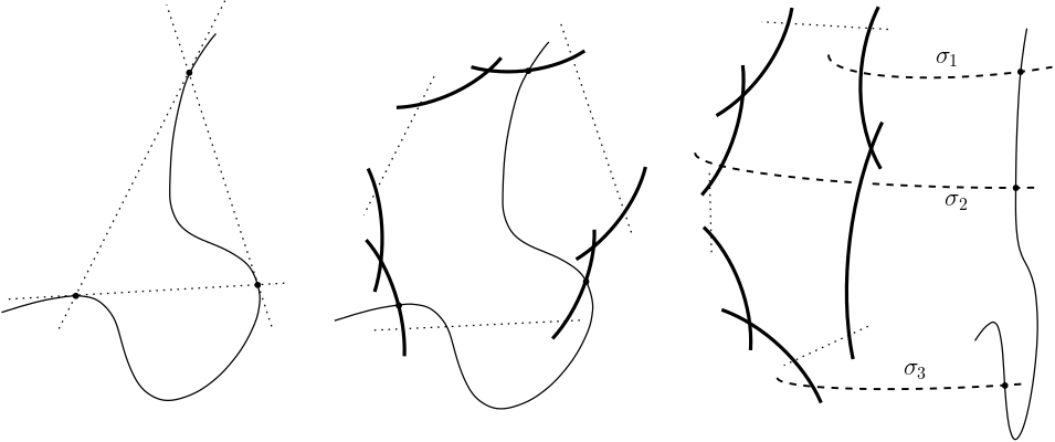
Figure 1. Construction of the rational elliptic surface $S$ with singular fibers $I_{9}+3A_{1}$.

Next, let $F$ be a smooth fiber of the elliptic fibration $S\to\mathbb{C}P^{1}$ obtained from the cubic pencil after the blow-ups, and take an isomorphism $H_{1}(F,\mathbb{Z})\cong\mathbb{Z}^{2}$. The monodromy of the fibration, which appears listed in No. 63 of [17, Table 3], is described by the equatlity $CX_{[1,-2]}X_{[2,-1]}A^{9}=\mathrm{I}$ (the reverse order is due to the fact that we are understanding the matrices as composition of endomorphisms). The notation is $X_{[p,q]}=\left(\begin{array}[]{cc}1+pq&-p^{2}\\ q^{2}&1-pq\end{array}\right)$, and $A=X_{[1,0]}$, $C=X_{[1,1]}$. So the monodromy representation is written as

$$\left(\begin{array}[]{cc}2&-1\\ 1&0\end{array}\right)\left(\begin{array}[]{cc}-1&-1\\ 4&3\end{array}\right)\left(\begin{array}[]{cc}-1&-4\\ 1&3\end{array}\right)\left(\begin{array}[]{cc}1&-1\\ 0&1\end{array}\right)^{9}=\mathrm{I}.$$

The vanishing cycle of $X_{[p,q]}$ is $(p,q)$, with the choice of path to the critical point taken in [17]. Therefore monodromies corresponding to going around the nodal curves are $C=X_{[1,1]}$, $X_{[1,-2]}$ and $X_{[2,-1]}$, whence the vanishing cycles are $(1,1)$, $(1,-2)$ and $(2,-1)$.

We take two copies $S_{1},S_{2}$ of $S$ as above, with two smooth fibers $F_{1},F_{2}$. They have $F_{1}^{2}=F_{2}^{2}=0$. We choose a symplectomorphism $\varphi:F_{1}\to F_{2}$ such that the vanishing cycles match, that is, the identity in homology $\varphi_{*}:H_{2}(F_{1},\mathbb{Z})\to H_{2}(F_{2},\mathbb{Z})$. Take the Gompf symplectic sum

$$X=S_{1}\#_{F_{1}=F_{2}}S_{2}=(S_{1}-\nu(F_{1}))\cup_{\nu(F_{1})-F_{1}\cong\nu(F_{2})-F_{2}}(S_{2}-\nu(F_{2}))\,.$$

As $b_{2}(S_{1})=b_{2}(S_{2})=10$, then $\chi(S_{1})=\chi(S_{2})=12$. So $\chi(X)=24$ and hence $b_{2}(X)=22$.

Let $C_{1},\ldots,C_{9}$ be the $I_{9}$-cycle of $S_{1}$, with sections $\sigma_{1},\sigma_{2},\sigma_{3}$ as before. Analogously, let $C^{\prime}_{1},\ldots,C^{\prime}_{9}$ be the $I_{9}$-cycle of $S_{2}$, with sections $\sigma^{\prime}_{1},\sigma^{\prime}_{2},\sigma^{\prime}_{3}$ as before. By using [25, Lemma 24], we can glue the sections to produce symplectic surfaces $E_{1},E_{2},E_{3}$ of square $(-2)$.

Lemma 13.

$X$ is simply connected.

Proof.

$S_{1}$ is simply connected, hence $\pi_{1}(S_{1}-\nu(F_{1}))$ is generated by a loop around $F_{1}$. But this is contracted by using one of the sections of the elliptic fibration. Hence $\pi_{1}(S_{1}-\nu(F_{1}))=1$. Also $\pi_{1}(S_{2}-\nu(F_{2}))=1$, so $\pi_{1}(X)=1$. ∎

Fix a fiber $F\subset\partial\nu(F_{1})=\partial\nu(F_{2})\subset X$. Take the vanishing cycle $a=(1,1)$ in $F$, and the two vanishing thimbles $D_{1},D_{2}$ in $S_{1}-\nu(F_{1}),S_{2}-\nu(F_{2})$, respectively. We glue them to form a Lagrangian $(-2)$-sphere $D$. Next take as dual curve in $F$ the curve $b=(1,-2)$, intersecting $a$ transversally and positively at three points. This follows since in $H_{1}(F_{0},\mathbb{Z})$, we have $\langle a,b\rangle=\langle(1,1),(1,-2)\rangle=3$, since the intersection form is antisymmetric. Take the torus $T=b\times S^{1}\subset F\times S^{1}=\partial\nu(F_{1})=\partial\nu(F_{2})$. This produces a pair of surfaces $D,T$ with

$$D^{2}=-2,\,D\cdot T=3,\,T^{2}=0,$$ (4)

where $D$ is a Lagrangian sphere and $T$ is a Lagrangian torus.

With the second vanishing cycle $b=(1,-2)$, we do the same thing using another fiber $F^{\prime}\subset\partial\nu(F_{1})=\partial\nu(F_{2})\subset X$. We obtain a pair $D^{\prime},T^{\prime}$ of Lagrangian $(-2)$-sphere and Lagrangian torus, disjoint from $D,T$. To arrange this, first move the $S^{1}$-factor in $\partial\nu(F_{1})=F_{1}\times S^{1}$, which maps to $S^{1}\subset\mathbb{C}P^{1}$ around the point giving the fiber $F_{1}$, in outward direction to make it disjoint. This produces that $T,T^{\prime}$ are disjoint. Second, note that the vanishing thimbles $D,D^{\prime}$ map to paths from the point defining the fiber to the point of the nodal fiber, and these can be made disjoint; third, to avoid the possible intersections $D\cap T^{\prime},D^{\prime}\cap T$ we use the dual curve to one of the vanishing cycle, which is equal to the other vanishing cycle, and move these loops in a parallel direction along $F$. Finally we use Lemma 12 to change slightly the symplectic form so that $D,D^{\prime}$ become symplectic $(-2)$-surfaces, and $T,T^{\prime}$ become symplectic tori.

Next, we see that there is a chain of $17$ rational $(-2)$-curves

$${\mathcal{C}}=C_{8}\cup\ldots\cup C_{2}\cup C_{1}\cup E_{1}\cup C_{1}^{\prime}\cup C_{2}^{\prime}\cup\ldots\cup C_{8}^{\prime}\,,$$

where $E_{1}$ is defined before Lemma 13 (see Figure 2). We contract $D$ and $D^{\prime}$ to two points $p,p^{\prime}$ of multiplicity $2$. Using Proposition 11, we contract the chain ${\mathcal{C}}$ to a point $q$ of multiplicity $18$. Note that $[2,\stackrel{{\scriptstyle(17)}}{{\ldots}},2]=\frac{18}{17}$, so the point has local model $(z_{1},z_{2})\mapsto(\varepsilon z_{1},\varepsilon^{-1}z_{2})$, with $\varepsilon=e^{2\pi i/18}$. Denote $\bar{X}$ the resulting symplectic cyclic orbifold with singular set $P=\{p,p^{\prime},q\}$. It has $b_{2}(\bar{X})=22-2-17=3$, and it is simply connected.

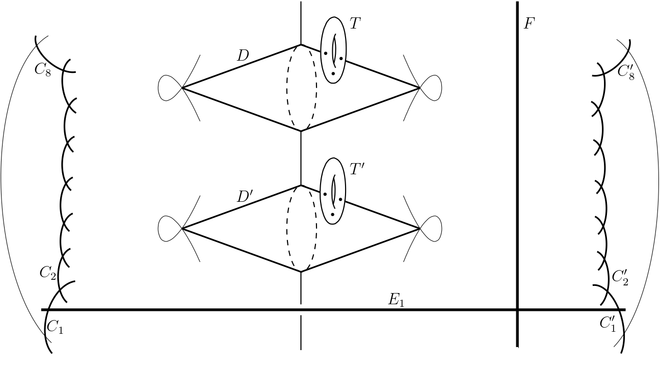
Figure 2. The $4$-manifold $X$ and all the surfaces constructed along the text.

Proposition 14.

There is a collection of smooth symplectic surfaces $T_{n}$, $n\geq 1$, in a neigbourhood of $T\cup D$, of genus $g_{n}=9n^{2}+1$, not intersecting $D$, and such that all the $T_{n}$ intersect pairwise nicely.

Proof.

Let $K$ be the canonical class of the symplectic form. Note that $K\cdot T=0$, $K\cdot D=0$, hence $K\cdot(aD+bT)=0$, for any $a,b\geq 0$.

We start constructing a curve $T_{1}\equiv 2T+3D$ as follows. By the symplectic neighbourhood theorem (Proposition 11), we can assume that we have a holomorphic model consisting of complex curves $D,T$ in a complex surface. Let $q_{1},q_{2},q_{3}$ be the points of $T\cap D$. We arrange two parallel copies of $T$, say $T^{\prime},T^{\prime\prime}$, which intersect transversely $D$ at six points $q_{1}^{\prime},q_{2}^{\prime},q_{3}^{\prime},q_{1}^{\prime\prime},q_{2}^{\prime\prime},q_{3}^{\prime\prime}$, where $q_{i}^{\prime},q_{i}^{\prime\prime}\in D$ are close to $q_{i}$, for $i=1,2,3$. Take the normal bundle to $D=\mathbb{C}P^{1}$, which is $\mathcal{O}_{D}(-2)$. Take three meromorphic sections $\sigma_{1},\sigma_{2},\sigma_{3}$ of $\mathcal{O}_{D}(-2)$, where $\sigma_{i}$ has poles at the points $q_{i}^{\prime},q_{i}^{\prime\prime}$. At each of the six points we do as follows, we do it with $q_{1}^{\prime}$ for concreteness. Take an adapted chart $(z,w)$ around $q_{1}^{\prime}$, where $T^{\prime}=\{z=0\}$, $D=\{w=0\}$. Around $q_{1}^{\prime}$ we can assume that $\sigma_{1}=1/z$. We glue the graph $\{(z,1/z)\}$ with the graph $\{(1/w,w)\}$ in the normal bundle to $T^{\prime}$ (which is trivial). We use a cut off function to push this graph down to the graph $T^{\prime}=\{(0,w)\}$, as in [8, Section 3.5]. The result is a symplectic surface. This has some self-intersections, which come from the intersections of the sections $\sigma_{1},\sigma_{2},\sigma_{3}$. These can be resolved symplectically to get a smooth symplectic surface of genus $g_{1}=10$, as in [25, Section 5.1] (basically changing the model $xy=0$ by $xy=\epsilon$). Note that $2g_{1}-2=T_{1}^{2}=(2T+3D)^{2}=12\cdot 3+9\cdot(-2)=18$. The surface $T_{1}$ does not intersect $D$. Note that $T_{1}\cdot D=(2T+3D)\cdot D=6-6=0$.

For given $n\geq 2$, take a collection of symplectic surfaces $\Sigma_{1},\ldots,\Sigma_{n}$ as graphs in the normal bundle to $T_{1}$, and all intersecting transversally and positively. Using [25, Section 5.1], we can glue symplectically the $\Sigma_{i}$, $1\leq i\leq n$, at the intersection points $\Sigma_{i}\cap\Sigma_{j}$ to obtain a symplectic surface $T_{n}\equiv\Sigma_{1}+\ldots+\Sigma_{n}\equiv nT_{1}$. Then $T_{n}^{2}=18n^{2}$ and the genus $g_{n}=9n^{2}+1$ satisfies $2g_{n}-2=18n^{2}$ since $K\cdot T_{n}=0$. Moreover, if we have different curves $T_{n}$, all can be taken to intersect transversally, and after perturbation as in Lemma 9, the intersections can be arranged to be nice. ∎

Proposition 15.

Let $F$ be a fiber of the fibration that intersects the chain ${\mathcal{C}}$ transversally at a point of $E_{1}$. Consider the configuration of symplectic surfaces ${\mathcal{C}}\cup F$. Then there is a symplectic surface $A$ of genus $g_{A}=10$, in a neighbourhood of ${\mathcal{C}}\cup F$, not intersecting the chain.

Proof.

Take a cohomology class of the form:

$$A\equiv 2F+a_{0}\sigma+a_{1}(C_{1}+C_{1}^{\prime})+a_{2}(C_{2}+C_{2}^{\prime})+\ldots+a_{8}(C_{8}+C_{8}^{\prime}).$$

to arrange that it is disjoint from the curves $E_{1}$ and $C_{i},C_{i}^{\prime}$, we need $0=A\cdot E_{1}=2-2a_{0}+2a_{1}$, $0=A\cdot C_{1}=a_{0}-2a_{1}+a_{2}$, $0=A\cdot C_{i}=a_{i-1}-2a_{i}+a_{i+1}$, $2\leq i\leq 7$, and $0=A\cdot C_{8}=a_{7}-2a_{8}$, whose solution is $a_{8}=1,a_{7}=2,\ldots,a_{1}=8,a_{0}=9$. Note that

$$A^{2}=4a_{0}+\sum 4a_{k-1}a_{k}-2a_{0}^{2}-\sum 4a_{k}^{2}=18,$$

hence $2g-2=K\cdot A+A^{2}=18$, so $g=10$.

To construct the curve $A$, consider the push-down map $\pi:X\to\bar{X}$, which contracts ${\mathcal{C}}$ to the singularity $q$. The image $A=\pi(A)$ should be a smooth symplectic curve avoiding the singular point. We denote by the same letter since it does not pass through the singular point. We construct $A$ directly in $\bar{X}$. As noted before, the singularity $q$ is cyclic of order $18$, and of type $\mathbb{C}^{2}/(\varepsilon,\varepsilon^{-1})$, $\varepsilon=e^{2\pi i/18}$. As explained in [28], there are $18$ affine charts covering the $17$ rational curves plus the coordinate axis $L_{1}=\{y=0\}$, $L_{2}=\{x=0\}$ (expressed in coordinates $(x,y)$). Each of these charts is centered at a point of intersection of two consecutive curves in the chain. They are given by the coordinates:

$$(\xi_{0},\eta_{0})=(x^{18},y/x^{17}),\,(\xi_{1},\eta_{1})=(x^{17}/y,y^{2}/x^{16}),\,(\xi_{2},\eta_{2})=(x^{16}/y^{2},y^{3}/x^{15}),\ldots$$

$$\ldots,(\xi_{8},\eta_{8})=(x^{10}/y^{8},y^{9}/x^{9}),\,(\xi_{9},\eta_{9})=(x^{9}/y^{9},y^{10}/x^{8}),\ldots$$

$$\ldots,(\xi_{16},\eta_{16})=(x^{2}/y^{16},y^{17}/x),\,(\xi_{17},\eta_{17})=(x/y^{17},y^{18}).$$

The axis $L_{1}$ is $\eta_{0}=0$ (i.e. $y=0$). The $(i+1)$-th curve in the chain is defined by $\xi_{i}=0$, $i=0,\ldots,16$. The second axis $L_{2}$ is $\xi_{17}=0$ (i.e. $x=0$). The curve $\bar{F}=\pi(F)$ passing through the mid-point of the $9$-th curve is given by the equation $\eta_{8}=1$, that is $y^{9}/x^{9}=1$. This is equivalent to $y^{9}-x^{9}=0$. The curve $2\bar{F}$ is thus $(y^{9}-x^{9})^{2}=0$, that we can perturb to a smooth curve as follows:

$$(y^{9}-x^{9})^{2}=\epsilon xy+\zeta,$$ (5)

with $0<\zeta\ll\epsilon\ll 1$, in the chart $\mathbb{C}^{2}/\mathbb{Z}_{18}$. This avoids the singular point (the origin), and it is easily seen to be smooth. It is $\mathbb{Z}_{18}$-equivariant, so it descends to a smooth curve. We have to glue it to two copies of $F$, therefore we have to see that the boundary (of the intersection of (5) with a ball in the affine chart around the singular point) is a collection of two circles. In this way we obtain the curve $A$ sought for.

For proving that the boundary of (5) consists of two circles, note that we can see this for $\zeta=0$, since the extra perturbation will merely move slightly the boundary, and so will not change it topologically. Note first that $y^{9}-x^{9}=0$ is a collection of $9$ lines, interchanged by $\mathbb{Z}_{18}$. Actually the image is the quotient of $y-x=0$ by $(x,y)\mapsto(-x,-y)$, which is the remaining $\mathbb{Z}_{2}$-action. Its boundary is the circle $\{(x,x)|x=e^{it}\}/(t\sim t+\pi)$. The equation $(y^{9}-x^{9})^{2}=0$ has as boundary again the same circle, but with multiplicity two. When we perturb $(y^{9}-x^{9})^{2}=\epsilon xy$, the curve $(x,y=x)$ gets moved to $(x,y=x+a(x))$, and we can compute easily a Taylor expansion

$$a(x)=\pm\frac{1}{9}\sqrt{\epsilon}\,x^{-7}+\frac{1}{162}\epsilon\,x^{-15}+\ldots$$

As we see, there are two solutions depending on the leading term. This means that there are two circles in the boundary (the other option would have been a double valued function $a(x)$). As there are only odd powers of $x$, the $\mathbb{Z}_{2}$-action $(x,y)\mapsto(-x,-y)$ goes down to $a\mapsto-a$, via $t\mapsto t+\pi$. That is, it acts on each circle, and not swapping the circles. So in the quotient, there are two circles remaining, as claimed. ∎

Take the push-down map $\pi:X\to\bar{X}$, which contracts $D,D^{\prime}$ to singularities $p,p^{\prime}$ and the chain ${\mathcal{C}}$ to the singularity $q$. Consider the collection of symplectic surfaces $T_{n}$, $1\leq n\leq N$, and $T^{\prime}_{m}$, $1\leq m\leq N$, and the symplectic surface $A=\pi(A)$. We shall fix a large $N>0$ later on. None of the surfaces pass through singular points. We arrange all intersections to be nice, so that we can assign coefficients to all surfaces and make $\bar{X}$ into a cyclic orbifold $X^{\prime}$ by using Proposition 3. We can assign local invariants by using Proposition 4.

We take coefficients as follows. The genus of $T_{n}$ and $T_{n}^{\prime}$ is $g_{n}=9n^{2}+1$, $n\geq 1$. For each $1\leq n,m\leq N$, take a prime $p_{nm}$. The collection of chosen primes should be different, $p_{nm}>3$ and satisfy $p_{nm}>n,m$. We assign multiplicities as follows:

$$m_{T_{n}} =\prod_{m=1}^{N}p_{nm},$$

$$m_{T_{m}^{\prime}} =\prod_{n=1}^{N}p_{nm}^{2}\,,$$

$$m_{A} =\prod_{n,m=1}^{N}p_{nm}^{3}\,.$$

Note that for $T_{n},T_{s}$, $n\neq s$, which are intersecting surfaces, we have that the primes $p_{nk},p_{sl}$ are different, hence $\gcd(m_{T_{n}},m_{T_{s}})=1$. Analogously, $\gcd(m_{T_{m}^{\prime}},m_{T_{l}^{\prime}})=1$, for $m\neq l$. Also note that $\gcd(m_{T_{n}},m_{A})\neq 1$ and $\gcd(m_{T_{m}^{\prime}},m_{A})\neq 1$, for all $n,m\geq 1$. Also for any $n,m$, $p_{nm}$ divides $m_{T_{n}}$ and $m_{T_{m}^{\prime}}$, hence $\gcd(m_{T_{n}},m_{T_{m}^{\prime}})\neq 1$. This is in accordance with the fact that the involved surfaces are disjoint.

Theorem 16.

For any $N\geq 1$, there is a Seifert bundle $\pi:M\to X^{\prime}$ which is K-contact and satisfies $H_{1}(M,\mathbb{Z})=0$ and

$$H_{2}(M,\mathbb{Z})=\mathbb{Z}^{2}\oplus\bigoplus_{n,m=1}^{N}\left(\mathbb{Z}_{p_{nm}}^{18n^{2}+2}\oplus\mathbb{Z}_{p_{nm}^{2}}^{18m^{2}+2}\oplus\mathbb{Z}_{p_{nm}^{3}}^{20}\right).$$

Moreover, $M$ is spin.

Proof.

We need to check the conditions of Proposition 6. First clearly $H_{1}(\bar{X},\mathbb{Z})=0$ because $\pi_{1}(\bar{X})=1$, by Lemma 13. Second we have to see the surjectivity of the map $H^{2}(\bar{X},\mathbb{Z})\to\oplus_{i}H^{2}(D_{i},\mathbb{Z}_{m_{i}})$. For this, we look at every prime. Let $p=p_{nm}$ and look at the map

$$\varpi:H^{2}(\bar{X},\mathbb{Z})\to H^{2}(T_{n},\mathbb{Z}_{p})\oplus H^{2}(T_{m}^{\prime},\mathbb{Z}_{p^{2}})\oplus H^{2}(A,\mathbb{Z}_{p^{3}}).$$

Recall that $T_{n}\equiv nT_{1}$, $T_{m}^{\prime}\equiv mT^{\prime}_{1}$, $A\equiv 2\bar{F}$ in $H_{2}(\bar{X},\mathbb{Z})$. The image $\varpi(T_{1})=(nT_{1}\cdot T_{1},0,0)=(18n,0,0)$, $\varpi(T_{1}^{\prime})=(0,mT^{\prime}_{1}\cdot T_{1}^{\prime},0)=(0,18m,0)$, $\varpi(A)=(0,0,A^{2})=(0,0,18)$, noting that $T_{1},T_{1}^{\prime},A\in H^{2}(\bar{X},\mathbb{Z})=H_{2}(\bar{X}-P,\mathbb{Z})$. Now $n,m$ are coprime with $p$ (since $p>n,m$) and $p\geq 5$ so that $\gcd(p,18)=1$.

To proceed, we need to choose $c_{1}(M)\in H^{2}(\bar{X},\mathbb{Q})$ so that it is a symplectic class, and also $c_{1}(M/\mathbb{Z}_{\mu})\in H^{2}(\bar{X}-P,\mathbb{Z})$ is primitive. This follows from Lemma 7 if we can assure that

$$x=\mu\left(\sum\frac{b_{n}}{m_{T_{n}}}[T_{n}]+\sum\frac{b^{\prime}_{m}}{m_{T_{m}^{\prime}}}[T^{\prime}_{m}]+\frac{b}{m_{A}}[A]\right)\in H^{2}(\bar{X}-P,\mathbb{Z})$$

is primitive, where $b_{n},b_{n}^{\prime}$, $n\geq 1$ and $b$ are the correponding $b_{i}$ associated to the local invariants. Note that $\mu=m_{A}=\prod_{n,m}p_{nm}^{3}$. If we choose $b=1$, then the coefficient of $[A]$ is $1$. Cupping with $[A]\in H_{2}(\bar{X}-P,\mathbb{Z})$, we obtain $\langle x,[A]\rangle=[A]^{2}=18$. So the only possible divisors of $x$ are $2$ or $3$. Now we note that $T_{n}\equiv nT_{1}$. Then the coefficient of $T_{1}$ in $x$ is

$$\frac{b_{1}\mu}{m_{T_{1}}}+\sum_{n\geq 2}\frac{b_{n}\mu n}{m_{T_{n}}}\,.$$

As $\mu$ is not divisible by $6$, if we choose $b_{1}=1$ and $b_{n}$ divisible by $6$ for $n\geq 2$, then this number is coprime with $6$. Then $x$ is not divisible by $2$ or $3$, as required.

By [18, equation (14)], the second Stiefel-Whitney class of $M$ is

$$w_{2}(M)=\pi^{*}w_{2}(\bar{X}-P)+\sum(m_{i}-1)\pi^{-1}(D_{i})\,.$$

As all $m_{i}$ are odd, then $w_{2}(M)=\pi^{*}w_{2}(\bar{X}-P)$. Note that $K\cdot T=0$, $K\cdot T^{\prime}=0$, $K\cdot A=0$, hence $K=0$, and so $w_{2}(\bar{X}-P)=0$ hence $w_{2}(M)=0$. So $M$ is spin. ∎

Finally, we compute the fundamental group.

Theorem 17.

The orbifold fundamental group $\pi_{1}^{\scriptsize\mathrm{orb}}(X^{\prime})=1$, and $\pi_{1}(M)=1$.

Proof.

Recall that $X$ is simply connected by Lemma 13, and that we contract the surfaces $D,D^{\prime}$ and the chain ${\mathcal{C}}$. The singular points of the orbifold $\bar{X}$ are $P=\{p,p^{\prime},q\}$. Then the fundamental group of

$$X^{o}=X-(D\cup D^{\prime}\cup{\mathcal{C}})=\bar{X}-P$$

is generated by loops around the singular points, that is $a,a^{\prime}$ around $p,p^{\prime}$, respectively, and $b$ around $q$. Note that $a^{2}=1,a^{\prime 2}=1,b^{18}=1$.

First fix a smooth fiber $F_{0}$. Recall that the vanishing cycles in $F_{0}$ are $(1,1)$, $(1,-2)$, $(2,-1)$. Let $\alpha,\beta\in\pi_{1}(F_{0})$ be the standard generators of the torus $F_{0}$. The third vanishing cycle contracts without touching any of the curves, because the vanishing thimbles can be taken to be disjoint. Hence $\alpha^{2}\beta^{-1}=1$ in $\pi_{1}(X^{o})$, so $\beta=\alpha^{2}$ and the group generated by $\alpha,\beta$ is generated by $\alpha$ and it is abelian.

Next, take the surface $A$ which lies in a neighbourhood of $F\cup{\mathcal{C}}$, and has genus $10$, and self-intersection $A^{2}=18$. Let $\alpha_{1},\beta_{1},\ldots,\alpha_{10},\beta_{10}$ be the loops generating $\pi_{1}(A)$ and let $\gamma$ be a small loop around $A$, that is, a meridian. We order the loops so that $\alpha_{1},\beta_{1},\alpha_{2},\beta_{2}$ homotop to $\alpha,\beta$ in the fiber $F$, and the other $\alpha_{j},\beta_{j}$ are close to the singular point, so of the form $b^{k}$ for some $k$ (the value $k$ depending on the loop). Then $\gamma^{18}=\prod_{j=1}^{10}[\alpha_{j},\beta_{j}]=1$. Adding the relation $\gamma^{m_{A}}$, and recalling that $\gcd(m_{A},18)=1$ (since we have chosen all primes $p>3$), we get $\gamma=1$ in $\pi_{1}^{\scriptsize\mathrm{orb}}(X^{\prime})$.

Now the fiber $F_{0}$ intersects the chain ${\mathcal{C}}$ in the central curve $E_{1}$. Note that the loops around the curves $C_{8},\ldots,C_{1},E_{1},C_{1}^{\prime},\ldots,C_{8}^{\prime}$ are given as, in this order, $b,\ldots,b^{8},b^{9},b^{10},\ldots,b^{17}$. Then the loop around $E_{1}$ is $b^{9}$, which produces the relation $b^{9}=[\alpha,\beta]=1$. Now we use the fact that there are two extra sections $E_{2}$, $E_{3}$ of the fibration. These avoid $T,D,T^{\prime},D^{\prime}$, $E_{2}$ intersects $C_{4},C_{4}^{\prime}$, and $E_{3}$ intersects $C_{7},C_{7}^{\prime}$. They intersect $A$ in two points. The loop around $A$ is trivial $\gamma=1\in\pi_{1}^{\scriptsize\mathrm{orb}}(X^{\prime})$. So we get relations $b^{5}=b^{13}$ and $b^{2}=b^{16}$. So $b^{8}=1$, that together with $b^{9}=1$ imply that $b=1$.

Finally take the surfaces $T_{n}$, $n\geq 1$, lying in a neighbourhood of $T\cup D$. Let $c_{j}$ be a small loop around $T_{j}$, $j\geq 0$, and recall that $a$ is a small loop around $D$, and $a^{2}=1$. All curves $T_{j}$ intersect transversally, so $[c_{j},c_{k}]=1$, for all $j,k$. Let $c_{0}$ be a small loop around $T$, then $c_{0}=a^{3}=a$, since $T\cdot D=3$. Move $T$ slightly off to get a relation $c_{1}^{9}c_{2}^{18}\ldots c_{N}^{9N}a=[\alpha\beta^{-2},\gamma]=1$ (the last loops are the generators of $\pi_{1}(T)$), using that $T\cdot T_{k}=9k$. The group generated by $a,c_{1},\ldots,c_{N}$ is abelian. We write the relations additively,

$$9(c_{1}+2c_{2}+\ldots+Nc_{N})+a=0.$$ (6)

Put for brevity, $m_{j}=m_{T_{j}}$. In $\pi_{1}^{\scriptsize\mathrm{orb}}(X^{\prime})$ we have the extra relations $m_{j}c_{j}=0$. Multiply (6) by $M_{k}=\prod_{j\neq k}m_{j}$ to get $9M_{k}kc_{k}=0$. Now $m_{k}c_{k}=0$, and $\gcd(m_{k},M_{k})=1$ since $\gcd(m_{j},m_{k})=1$ for $j\neq k$, and also $\gcd(k,m_{k})=1$ because we chose $\gcd(p_{km},k)=1$, and $m_{k}=\prod_{m}p_{km}$, and $\gcd(m_{k},3)=1$ as all primes are $p>3$. All together give $c_{k}=0$, for $k\geq 1$. Then (6) gives $a=0$ as well in $\pi_{1}^{\scriptsize\mathrm{orb}}(X^{\prime})$.

Once that $\pi_{1}^{\scriptsize\mathrm{orb}}(X^{\prime})=1$, we get $\pi_{1}(M)=0$ by the argument at the end of Section 2.4 using that $H_{1}(M,\mathbb{Z})=0$ from Theorem 16. ∎

Therefore the K-contact manifold from Theorem 16 is a Smale-Barden manifold.

4. Bounding the number of singular points

Our last step is to prove that the manifold $M$ from Theorem 16 does not admit a Sasakian structure. Suppose that $M$ admits a Sasakian structure. Then there is Seifert bundle

$$\pi:M\to Y,$$

where $Y$ satisfies the following conditions that we state explicitly:

Conditions 18.

$Y$ is a Kähler cyclic orbifold with $b_{2}=3$, $b_{1}=0$. Associated to each prime $p_{nm}$, $1\leq n,m\leq N$, there is a collection of three complex curves

$$D_{1}^{nm},D_{2}^{nm},D_{3}^{nm},$$ (7)

which have genus $g(D_{1}^{nm})=9n^{2}+1$, $g(D_{2}^{nm})=9m^{2}+1$, $g(D_{3}^{nm})=10$. For each $(n,m)$, the three curves (7) are disjoint, and span $H_{2}(Y,\mathbb{Q})$. Moreover, these curves are all nice, and intersect pairwise nicely.

This follows from the homology of $M$ appearing in Theorem 16 and the relation to the homology of the base of a Seifert bundle given in Proposition 6. The curves (7) are the components of the isotropy locus. Conditions 18 imply that at most two different curves can go through a point of the singular set $P\subset X$. Some of the curves could be equal for different values of $(n,m)$, e.g.  $D_{1}^{nk}=D_{1}^{nl}$, $k\neq l$; or $D_{2}^{km}=D_{2}^{lm}$, $k\neq l$; or $D_{1}^{nk}=D_{2}^{ln}$; or $D_{3}^{nm}=D_{3}^{kl}$. Clearly, this can only happen if the genera of the involved curves are the same.

To prove that $M$ cannot admit a Sasakian structure, we are going to get a contradiction if we assume the existence of a Kähler orbifold $Y$ satisfying Conditions 18, for some $N\gg 0$ large enough. After preparatory work in Sections 4, 5 and 6, this will be proved in Theorem 32 in Section 7.

To start with, let $Y$ be a Kähler cyclic orbifold satisfying Conditions 18. We do not assume $\pi_{1}^{\scriptsize\mathrm{orb}}(Y)=0$. Our first task is to obtain a universal bound on the number of singular points $\#P$.

Let $\pi:\tilde{Y}\to Y$ be the minimal resolution of singularities. For every cyclic singularity $p\in Y$, $\pi^{-1}(p)=E_{p}=C_{1}\cup\ldots\cup C_{l}$ is a chain of rational curves with self-intersection $C_{j}^{2}=-b_{j}\leq-2$. For any curve $A$ in $Y$, we denote the proper transform as $\tilde{A}$. Let $A$ be a nice curve through $p$ (for the sake of simplicity, assume that there is only one singular point). Then $\tilde{A}$ intersects transversely just one of the extremal curves of the chain $C_{1},C_{l}$. For concreteness, say it is $C_{1}$. We have that (see [3, p. 80])

$$\pi^{*}A=\tilde{A}+\sum r_{i}C_{i}\,,$$

where $\frac{r_{k+1}}{r_{k}}=[b_{k+1},\ldots,b_{l}]^{-1}$, for $0\leq k\leq l-1$, where $r_{0}=1$. Note that $\frac{r_{k+1}}{r_{k}}<1$, hence $0<r_{l}<r_{l-1}<\ldots<r_{1}<1$. Next, let $\tilde{K}$ be the canonical divisor of $\tilde{Y}$, and $K$ the canonical divisor of $Y$. In this case, $\tilde{K}$ is not the proper transform of $K$. We have a formula (again assuming only one singular point)

$$\tilde{K}=\pi^{*}K-\sum\lambda_{i}C_{i}\,,$$ (8)

where $\lambda_{i}\geq 0$. If there are more singular points, then we have to add the contribution over each $p\in P$.

Lemma 19.

Let $A,B$ be two effective divisors in $Y$, and let $\tilde{A},\tilde{B}$ be the proper transforms. Then $A\cdot B\geq\tilde{A}\cdot\tilde{B}$.

Proof.

It is enough to prove it for $A,B$ two irreducible curves in $Y$. Then

$$A\cdot B=\pi^{*}A\cdot\pi^{*}B=\pi^{*}A\cdot\tilde{B}=(\tilde{A}+E)\cdot\tilde{B}\geq\tilde{A}\cdot\tilde{B}.$$

The second equality follows since $\pi^{*}A\cdot C_{i}=A\cdot\pi_{*}C_{i}=0$, for any exceptional divisor $C_{i}$. The third, because $\pi^{*}A=\tilde{A}+E$, where $E=\sum r_{i}C_{i}$, where $r_{i}\in\mathbb{Q}$, $r_{i}\geq 0$, and $C_{i}$ are exceptional divisors. The last equality is due to $C_{i}\cdot\tilde{B}\geq 0$, being two distinct effective curves. ∎

Now let $D_{1},D_{2},D_{3}$ be three nice curves, which are disjoint, and span $H_{2}(Y,\mathbb{Q})$. We have the following:

Lemma 20.

The $\mathbb{Q}$-divisor $K+D_{1}+D_{2}+D_{3}$ is effective. Also $K+D_{i}$ is effective, $i=1,2,3$.

Proof.

We have the exact sequence

$$0\to\mathcal{O}(\tilde{K})\to\mathcal{O}(\tilde{K}+\tilde{D}_{1}+\tilde{D}_{2}+\tilde{D}_{3})\to\oplus\,\mathcal{O}_{\tilde{D}_{i}}(K_{\tilde{D}_{i}})\to 0,$$

because the $\tilde{D}_{i}$ are disjoint, and using the adjunction formula. As $g(\tilde{D}_{i})=g_{i}\geq 1$, $H^{0}(\mathcal{O}_{\tilde{D}_{i}}(K_{\tilde{D}_{i}}))=\mathbb{C}^{g_{i}}\neq 0$, by Riemann-Roch. As $b_{1}(\tilde{Y})=0$, so $H^{1}(\tilde{K})=0$. Also $H^{0}(\tilde{K})=0$, since $h^{0,2}(\tilde{Y})=0$, because $H^{2}(\tilde{Y},\mathbb{C})$ is spanned by complex curves, so $h^{1,1}(\tilde{Y})=b_{2}(\tilde{Y})$. Therefore $h^{0}(\mathcal{O}(\tilde{K}+\tilde{D}_{1}+\tilde{D}_{2}+\tilde{D}_{3}))=g_{1}+g_{2}+g_{3}>0$, and hence there is some effective divisor $\Sigma^{\prime}\equiv\tilde{K}+\tilde{D}_{1}+\tilde{D}_{2}+\tilde{D}_{3}$. Pushing down, $\Sigma=\pi(\Sigma^{\prime})\equiv K+D_{1}+D_{2}+D_{3}$ in $Y$.

The last assertion is proved in the same way. ∎

Put $B=D_{1}+D_{2}+D_{3}$. We need to check that $K+B$ is log canonical, whose definition appears in [21, Definition 1.16]. This is checked at each singular point $p\in P$. Suppose that $p\in D_{1}=D$ (the case that $p$ is not in any divisor $D_{i}$ is similar). Assume for simplicity that there are no more singular points, and write

$$\tilde{K}=\pi^{*}(K+D)-\tilde{D}+\sum_{i=1}^{l}a_{i}C_{i}\,,$$

where $\tilde{D}$ is the proper transform of $D$, $C_{i}$ are the exceptional divisors, ordered so that $\tilde{D}\cdot C_{1}=1$. We have to check that $a_{i}\geq-1$. Letting $a_{0}=-1$ the coefficient of $\tilde{D}$, and setting $a_{l+1}=0$, we have the equalities $\tilde{K}\cdot C_{i}+C_{i}^{2}=-2$, which give $-a_{i}b_{i}+a_{i-1}+a_{i+1}-b_{i}=-2$. This is rewriten as

$$(a_{i-1}-a_{i})+(a_{i+1}-a_{i})=(a_{i}+1)(b_{i}-2).$$ (9)

Let $i_{0}$ be such that $a_{i_{0}}$ is minimum. Then the left hand side of (9) for $i=i_{0}$ is $\geq 0$. Therefore if $b_{i_{0}}>2$, then $a_{i_{0}}+1\geq 0$, and so $a_{i}\geq a_{i_{0}}\geq-1$, for all $i$. If $b_{i_{0}}=2$ then $a_{i-1}=a_{i}=a_{i+1}$ and we proceed recursively.

Recall the definition of the orbifold Euler-Poincaré characteristic of an orbifold with isolated singularities,

$$e_{\scriptsize\mathrm{orb}}(Y)=e(Y)-\sum_{p\in P}\left(1-\frac{1}{d_{p}}\right),$$

where $d_{p}$ denotes the multiplicity of the singular point $p\in P$.

Theorem 21.

Now let $D_{1},D_{2},D_{3}$ be three disjoint nice curves that span $H_{2}(Y,\mathbb{Q})$. Then $e_{\scriptsize\mathrm{orb}}(Y-(D_{1}\cup D_{2}\cup D_{3}))\geq 0$.

Proof.

Let $B=D_{1}+D_{2}+D_{3}$. We already know that $(Y,B)$ is log canonical and effective. If we have that $K+B$ is nef, then [21, Theorem 10.14] implies that

$$3c_{2}(\Omega_{Y}^{1}(\log B))\geq c_{1}(\Omega_{Y}^{1}(\log B))^{2}=(K+B)^{2}\geq 0,$$

where the last inequality is due to the fact that $K+B$ is effective and nef. By [21, Theorem 10.8], we have that $c_{2}(\Omega_{Y}^{1}(\log B))=e_{\scriptsize\mathrm{orb}}(Y-B)$ and the result follows.

It remains to see that $K+B$ is nef. Let $A\subset Y$ be an irreducible curve, and let us check that $(K+B)\cdot A\geq 0$. First assume that $A=D_{i}$. By Lemma 19, $K+D_{i}$ is effective. Moreover $H^{0}(\tilde{K}+\tilde{D}_{i})\to H^{0}(\mathcal{O}_{\tilde{D}_{i}}(K_{\tilde{D}_{i}}))$ is bijective, and as $K_{\tilde{D}_{i}}$ is base-point free, $\tilde{K}+\tilde{D}_{i}$ can be represented by a divisor not containing $\tilde{D}_{i}$. Hence there is $C\equiv K+D_{i}$ not containing $D_{i}$, and thus $(K+B)\cdot A=(K+D_{i})\cdot D_{i}=C\cdot D_{i}\geq 0$.

So we can suppose now that $A\neq D_{i}$, $i=1,2,3$. Let $\Sigma\equiv K+B$ be an effective $\mathbb{Q}$-divisor. Write $\Sigma=rA+T$, where $T$ does not contain $A$. If $A^{2}\geq 0$ then $(K+B)\cdot A=\Sigma\cdot A\geq 0$, and we are done. So we can assume that $A^{2}<0$. By Lemma 19, we also have $\tilde{A}^{2}<0$.

Next suppose that $\tilde{K}\cdot\tilde{A}\geq 0$. Then as $K=\pi_{*}\tilde{K}$ (although $\tilde{K}$ is not the strict transform of $K$),

$$K\cdot A=\pi_{*}\tilde{K}\cdot A=\tilde{K}\cdot\pi^{*}A=\tilde{K}\cdot(\tilde{A}+E)\geq\tilde{K}\cdot\tilde{A}\geq 0,$$

where $E$ is an effective $\mathbb{Q}$-divisor consisting of exceptional curves $E=\sum r_{i}C_{i}$, $r_{i}\geq 0$. For any $C_{i}$, it is $\tilde{K}\cdot C_{i}\geq 0$, since they are rational curves with $C_{i}^{2}\leq-2$. As $B\cdot A\geq 0$ then $(K+B)\cdot A\geq 0$, as required.

So we are left with the case of an irreducible curve $\tilde{A}$ with $\tilde{A}^{2}<0$, $\tilde{K}\cdot\tilde{A}<0$. As $p_{a}(\tilde{A})=\tilde{A}^{2}+\tilde{K}\cdot\tilde{A}<0$, then $\tilde{A}$ must be a smooth rational curve, with $\tilde{A}^{2}=-1$ and $\tilde{K}\cdot\tilde{A}=-1$, that is an exceptional divisor for a minimal model of $\tilde{Y}$.

If $A\cdot D_{1}=A\cdot D_{2}=0$, then $A\equiv\lambda D_{3}$, for some $\lambda>0$, which is impossible since $A\cdot D_{3}\geq 0$ and $D_{3}^{2}<0$. If $A\cdot D_{2}=A\cdot D_{3}=0$, then $A\equiv\lambda D_{1}$, for some $\lambda>0$, and hence $A^{2}>0$, contrary to our current assumption. Finally, if $A\cdot D_{1}=0$, then $A\equiv\lambda_{2}D_{2}+\lambda_{3}D_{3}$, for some $\lambda_{i}\in\mathbb{Q}$. Since $A\cdot D_{i}\geq 0$, then $\lambda_{i}\leq 0$, $i=2,3$. Hence $A\leq 0$, which is a contradiction as $A$ is effective.

So we can assume $A\cdot D_{1}>0$ and $A\cdot D_{2}>0$ (after swapping $D_{2},D_{3}$ if necessary). Now $(\tilde{K}+\tilde{D}_{1}+\tilde{D}_{2}+\tilde{D}_{3})\cdot\tilde{A}=-1+\sum\tilde{D}_{i}\cdot\tilde{A}$. If $\tilde{D}_{i}\cdot\tilde{A}\geq 1$ for some $i$, then $(\tilde{K}+\tilde{D}_{1}+\tilde{D}_{2}+\tilde{D}_{3})\cdot\tilde{A}\geq 0$. Recall that there is an effective $\Sigma^{\prime}\equiv\tilde{K}+\tilde{D}_{1}+\tilde{D}_{2}+\tilde{D}_{3}$, with $\pi(\Sigma^{\prime})=\Sigma\equiv K+B$. So

$$(K+B)\cdot A=\Sigma^{\prime}\cdot\pi^{*}A=\Sigma^{\prime}\cdot(\tilde{A}+E)\geq 0,$$

where we have $E=\sum r_{i}C_{i}$, $r_{i}\geq 0$, and $\Sigma^{\prime}\cdot C_{i}\geq 0$ because $\tilde{D}_{j}\cdot C_{i}\geq 0$ and $\tilde{K}\cdot C_{i}\geq 0$.

Hence we can further assume that $\tilde{D}_{i}\cdot\tilde{A}=0$, for all $i$. As $A\cdot D_{1}>0$, $A\cdot D_{2}>0$, this means that $\tilde{A}$ intersects a chain of exceptional divisors $E_{p}$, for a singularity $p\in A\cap D_{i}$, for both cases $i=1,2$. By Lemma 19, we have

$$(K+D_{1}+D_{2}+D_{3}+A)\cdot A\geq(\tilde{K}+\tilde{D}_{1}+\tilde{D}_{2}+\tilde{D}_{3}+\tilde{A})\cdot\tilde{A}+\sum_{p\in P}\ell_{p}=-2+\sum_{p\in P}\ell_{p},$$

where $\ell_{p}$ denotes a local contribution of the intersection at $p$. There is contribution to $\ell_{p}$ only if $p\in A\cap D_{i}$. This happens at least for two singular points, hence it is enough to see that $\ell_{p}\geq 1$ if $p\in A\cap D_{i}$. Once we have checked that, we have that $(K+D_{1}+D_{2}+D_{3}+A)\cdot A\geq 0$. As we are assuming $A^{2}<0$, we have $(K+D_{1}+D_{2}+D_{3})\cdot A\geq 0$, i.e. $(K+B)\cdot A\geq 0$, completing the proof.

Let us finally see that $\ell_{p}\geq 1$. The proper transform $\tilde{A}$ intersects the chain $E_{p}=C_{1}\cup\ldots\cup C_{l}$, but not $\tilde{D}_{i}$. Let $\alpha_{j}=\tilde{A}\cdot C_{j}\in\mathbb{Z}_{\geq 0}$. Take (a germ of) a curve $A^{\prime}_{j}$ that intersects transversally $C_{j}$ and no other $C_{k}$. Then $\tilde{A}\equiv\sum\alpha_{j}A^{\prime}_{j}$ in a neighbourhood of $E_{p}$, and so $A\equiv\sum\alpha_{j}A_{j}$ where $A_{j}=\pi(A_{j}^{\prime})$. Then the contribution at $p$ is

$$\ell_{p}= \left((K+D_{1}+D_{2}+D_{3}+A)\cdot A\right)_{p}$$

$$= \left((K+D_{1}+D_{2}+D_{3}+\sum\alpha_{j}A_{j})\cdot\sum\alpha_{k}A_{k}\right)_{p}$$

$$= \sum\alpha_{j}\left((K+D_{1}+D_{2}+D_{3}+A_{j})\cdot A_{j}\right)_{p}$$

$$+\sum_{j\neq k}\alpha_{j}\alpha_{k}(A_{j}\cdot A_{k})_{p}+\sum(\alpha_{j}^{2}-\alpha_{j})(A_{j}^{2})_{p}\,.$$

The local intersection number is defined in [14]. As $(A_{j}\cdot A_{k})_{p}\geq 0$, we see that it is enough to prove the result for $A=A_{j}$. We assume this henceforth.

To compute $\left((K+D_{i}+A)\cdot A\right)_{p}$, note that $A$ only intersects $C_{j}$. We contract $C_{1}\cup\ldots\cup C_{j-1}$ and $C_{j+1}\cup\ldots\cup C_{l}$ and get an orbifold $\bar{Y}$, such that there are contractions $\tilde{Y}\to\bar{Y}\to Y$. The map $\varpi:\bar{Y}\to Y$ has an exceptional divisor $\bar{E}$ with two orbifold points $p_{1},p_{2}$ of multiplicities $d_{1},d_{2}$ respectively (it is $d_{1}=1$ if $j=1$, and $d_{2}=1$ if $j=l$). The proper transform of $D_{i}$ is $\bar{D}_{i}$ with $p_{1}=\bar{D}_{i}\cap\bar{E}$, which is a nice intersection. The proper transform of $A$, denoted $A$ again, intersects $\bar{E}$ transversally at a smooth point.

We have the following intersection numbers (see [14]). Let $\frac{a_{1}}{d_{1}}=[b_{j-1},\ldots,b_{1}]^{-1}$, $\frac{a_{2}}{d_{2}}=[b_{j+1},\ldots,b_{l}]^{-1}$ be the continuous fractions associated to the singularities (with $a_{j}=0$ if $d_{j}=1$), and let $\frac{a^{\prime}_{1}}{d_{1}}=[b_{1},\ldots,b_{j-1}]^{-1}$, $\frac{a^{\prime}_{2}}{d_{2}}=[b_{l},\ldots,b_{j+1}]^{-1}$ be the dual ones. Then, writing $b=b_{j}$,

$$(\bar{D}_{i}\cdot\bar{E})_{p_{1}} =\frac{1}{d_{1}}$$

$$\bar{E}^{2} =-b+\frac{a_{1}}{d_{1}}+\frac{a_{2}}{d_{2}}$$

$$(\bar{D}_{i}^{2})_{p_{1}} =\frac{a_{1}^{\prime}}{d_{1}}$$

Using the adjunction equality for a nice curve,

$$K_{\bar{Y}}\cdot C+C^{2}=-e_{\scriptsize\mathrm{orb}}(C)=2g(C)-2+\sum_{p\in C}\left(1-\frac{1}{d_{p}}\right),$$

the corresponding local contribution for $C=\bar{E},\bar{D}_{i}$, gives

$$K_{\bar{Y}}\cdot\bar{E} =b-\frac{a_{1}+1}{d_{1}}-\frac{a_{2}+1}{d_{2}}$$

$$(K_{\bar{Y}}\cdot\bar{D}_{i})_{p} =1-\frac{a_{1}^{\prime}+1}{d_{1}}$$

Recall that we aim to compute $\ell_{p}=\left((K+D_{i}+A)\cdot A\right)_{p}=\left((\bar{K}+\bar{D}_{i}+A)\cdot\varpi^{*}A\right)_{p}$, where the right hand side accounts for the contribution to the intersection along the exceptional divisor. We write $\varpi^{*}A=A+x\bar{E}$, and compute $x\in\mathbb{Q}$ knowing that $\varpi^{*}A\cdot\bar{E}=0$ and $A\cdot\bar{E}=1$. Then

$$x=-\frac{1}{\bar{E}^{2}}=\frac{d_{1}d_{2}}{bd_{1}d_{2}-a_{1}d_{2}-a_{2}d_{1}}\,,$$

and hence

$$\ell_{p} =\left((K+D_{i}+A)\cdot A\right)_{p}=\left((\bar{K}+\bar{D}_{i}+A)\cdot\varpi^{*}A\right)_{p}$$

$$=\left((\bar{K}+\bar{D}_{i}+A)\cdot(A+x\bar{E})\right)_{p}$$

$$=\left(b-\frac{a_{1}+1}{d_{1}}-\frac{a_{2}+1}{d_{2}}+\frac{1}{d_{1}}+1\right)\frac{d_{1}d_{2}}{bd_{1}d_{2}-a_{1}d_{2}-a_{2}d_{1}}$$

$$=1+\frac{d_{1}(d_{2}-1)}{bd_{1}d_{2}-a_{1}d_{2}-a_{2}d_{1}}\geq 1,$$

as required. ∎

By Theorem 21, the orbifold Euler-Poincaré characteristic is

$$e_{\scriptsize\mathrm{orb}}(Y-(D_{1}\cup D_{2}\cup D_{3}))=5-\sum(2-2g_{i})-\sum_{p\in Y\atop p\notin D_{1}\cup D_{2}\cup D_{2}}\left(1-\frac{1}{d_{p}}\right)\geq 0,$$

where $g_{1},g_{2},g_{3}$ are the genus of $D_{1},D_{2},D_{3}$, respectively. As $d_{p}\geq 2$, we deduce

$$\#\{p\in P,p\notin D_{1}\cup D_{2}\cup D_{2}\}\leq 2(2g_{1}+2g_{2}+2g_{3}-1).$$ (10)

Now let us have three collections of curves $(D_{1},D_{2},D_{3})$, $(D^{\prime}_{1},D^{\prime}_{2},D^{\prime}_{3})$, $(D^{\prime\prime}_{1},D^{\prime\prime}_{2},D^{\prime\prime}_{3})$ in the same situation, and suppose that all curves are distinct. Let $A=\{p\in P,p\in D_{1}\cup D_{2}\cup D_{3}\},A^{\prime}=\{p\in P,p\in D_{1}^{\prime}\cup D_{2}^{\prime}\cup D_{3}^{\prime}\},A^{\prime\prime}=\{p\in P,p\in D_{1}^{\prime\prime}\cup D_{2}^{\prime\prime}\cup D_{3}^{\prime\prime}\}$. If $p\in Y$, then it can be at most in two curves (since they intersect nicely). Therefere either $p\notin A,p\notin A^{\prime}$ or $p\notin A^{\prime\prime}$. So $P\subset(P-A)\cup(P-A^{\prime})\cup(P-A^{\prime\prime})$. By the equality (10) above,

$$\#P\leq 2(2g_{1}+2g_{2}+2g_{3}-1)+2(2g^{\prime}_{1}+2g^{\prime}_{2}+2g^{\prime}_{3}-1)+2(2g^{\prime\prime}_{1}+2g^{\prime\prime}_{2}+2g^{\prime\prime}_{3}-1),$$ (11)

where $g_{i},g_{i}^{\prime},g_{i}^{\prime\prime}$ denote the genus of the respective curves.

Corollary 22.

Suppose that we have five bases with genera $\{g_{1},g_{2},10\}$, $\{g_{1}^{\prime},g_{2}^{\prime},10\}$, $\{g_{1}^{\prime\prime},g_{2}^{\prime\prime},10\}$, $\{g_{1}^{\prime\prime\prime},g_{2}^{\prime\prime\prime},10\}$, $\{g_{1}^{\prime\prime\prime\prime},g_{2}^{\prime\prime\prime\prime},10\}$, and all $g_{1},g_{2}$, $g_{1}^{\prime},g_{2}^{\prime}$, $g_{1}^{\prime\prime},g_{2}^{\prime\prime}$, $g_{1}^{\prime\prime\prime},g_{2}^{\prime\prime\prime}$, $g_{1}^{\prime\prime\prime\prime},g_{2}^{\prime\prime\prime\prime}$ and $10$ are distinct numbers. Then there is some $\tau_{0}$ (independent of $Y$) such that $\#P\leq\tau_{0}$.

Proof.

For checking this, we use Definition 23 from upcoming Section 5 (the results that we use for this proof are independent of Section 5). If among the five curves of genus $10$, say $D_{3},D_{3}^{\prime},D_{3}^{\prime\prime},D_{3}^{\prime\prime\prime},D_{3}^{\prime\prime\prime\prime}$, there are only two distinct curves, then three of them coincide. Suppose that $D_{3}=D_{3}^{\prime}=D_{3}^{\prime\prime}$. Then Lemma 25 (below) implies that two of the bases (say $\varepsilon,\varepsilon^{\prime}$) are proj-equivalent, and hence $D_{2}^{\prime}=\lambda_{2}D_{2}$, with $\lambda_{2}>0$. As $D_{2}\neq D_{2}^{\prime}$ because they have different genus, we get $D_{2}\cdot D_{2}^{\prime}\geq 0$. But then $\lambda_{2}D_{2}^{2}\geq 0$, which is a contradiction, as $D_{2}^{2}<0$.

Therefore there are three of the bases with all curves distinct, and we take $\tau_{0}$ as the right hand side of the formula (11). ∎

The assumption of Corollary 22 is achieved as soon as we take $N\geq 11$ for (7).

5. Many collections of orthogonal bases of curves

Let $Y$ be a Kähler cyclic orbifold with $b_{1}=0$ and $b_{2}=3$. Let $P$ be the collection of singular points. Suppose that the ramification locus consists of a collection of nice curves $D_{i}^{(k)}$, $i=1,2,3$, $1\leq k\leq K$, such that

$$\varepsilon^{(k)}=(D_{1}^{(k)},D_{2}^{(k)},D_{3}^{(k)})$$ (12)

are orthogonal bases for $H_{2}(Y,\mathbb{Q})$, formed by curves which are disjoint. As $Y$ is a Kähler orbifold, $h^{1,1}(Y)=b_{2}(Y)=3$, because the homology is spanned by complex curves. The intersection form of $H^{2}(Y,\mathbb{R})$ is of signature $(1,2)$. So we can order the curves so that $(D_{1}^{(k)})^{2}=m_{1}^{(k)}>0$, $(D_{2}^{(k)})^{2}=-m_{2}^{(k)}<0$, $(D_{3}^{(k)})^{2}=-m_{3}^{(k)}<0$. The genera are $g_{1}^{(k)}=g(D_{1}^{(k)}),g_{2}^{(k)}=g(D_{2}^{(k)}),g_{3}^{(k)}=g(D_{3}^{(k)})\geq 1$.

For $k\neq l$, it may happen that $D_{i}^{(k)}=D_{j}^{(l)}$ in which case $g_{i}^{(k)}=g_{j}^{(l)}$, and also either $i=j=1$ or $i,j\in\{2,3\}$ (since the self-intersection coincides). On the other hand, if the curves are distinct then it must be $D_{i}^{(k)}\cdot D_{j}^{(l)}\geq 0$.

Definition 23.

Let $\varepsilon=\big{(}D_{1},D_{2},D_{3}\big{)}$, $\varepsilon^{\prime}=\big{(}D^{\prime}_{1},D_{2}^{\prime},D^{\prime}_{3}\big{)}$ be two bases from the above list. We write $[\varepsilon]=[\varepsilon^{\prime}]$ if the elements are proportional, that is up to reordering, $D_{i}^{\prime}=\lambda_{i}D_{i}$ with $\lambda_{i}>0$. We say that the bases are proj-equivalent.

Note that if $[\varepsilon]=[\varepsilon^{\prime}]$ then, by the discussion above, we have that $D_{2}=D_{2}^{\prime}$ and $D_{3}=D_{3}^{\prime}$.

Let $K$ be the orbifold canonical class of $Y$. Let $\varepsilon=(D_{1},D_{2},D_{3})$ be one of the basis provided above. Then we write $K=\sum a_{i}D_{i}$. We have the orbifold adjunction equality

$$K\cdot D+D^{2}=-e_{\scriptsize\mathrm{orb}}(D),$$

for a smooth orbifold (nice) curve $D\subset Y$. As $b^{+}_{2}=1$, we have that $D_{1}^{2}=m_{1}>0$, $D_{i}^{2}=-m_{i}<0$ for $i=2,3$, where $m_{i}\in\mathbb{Q}$. Let $g_{i}$ be the genus of $D_{i}$. Let

$$\chi_{i}=-e_{\scriptsize\mathrm{orb}}(D_{i})=2g_{i}-2+\sum_{p\in D_{i}}\left(1-\frac{1}{d_{p}}\right),$$

where $d_{p}$ is the order of the singular point $p\in D_{i}$. Then $\chi_{i}\geq 2g_{i}-2$. Using the adjunction formula, then $a_{1}=(\chi_{1}-m_{1})/m_{1}$, $a_{i}=-(\chi_{i}+m_{i})/m_{i}$ for $i=2,3$, so

$$K=\frac{\chi_{1}-m_{1}}{m_{1}}D_{1}-\frac{\chi_{2}+m_{2}}{m_{2}}D_{2}-\frac{\chi_{3}+m_{3}}{m_{3}}D_{3}\,.$$ (13)

Note that $\chi_{i}+m_{i}>0$ for $i=2,3$.

By Lemma 20, $K+D_{2}$ is effective. But

$$K+D_{2}=\frac{\chi_{1}-m_{1}}{m_{1}}D_{1}-\frac{\chi_{2}}{m_{2}}D_{2}-\frac{\chi_{3}+m_{3}}{m_{3}}D_{3}\,.$$

If $m_{1}\geq\chi_{1}$, then this is anti-effective, which is a contradiction. Hence we always have

$$0<m_{1}<\chi_{1}.$$ (14)

Lemma 24.

Let $\varepsilon=\big{(}D_{1},D_{2},D_{3}\big{)}$, $\varepsilon^{\prime}=\big{(}D^{\prime}_{1},D_{2}^{\prime},D^{\prime}_{3}\big{)}$ be two bases. If $D_{1}^{\prime}=\lambda_{1}D_{1}$, then $[\varepsilon]=[\varepsilon^{\prime}]$. In particular, $D_{2}=D_{2}^{\prime}$ and $D_{3}=D_{3}^{\prime}$.

Proof.

We restrict to $V=\langle D_{1}\rangle^{\perp}\subset H_{2}(Y,\mathbb{R})$, which is a vector space with a (negative) definite scalar product. If $D_{2}=\lambda_{2}D_{2}^{\prime}$ (up to reordering), then it must be $D_{3}=\lambda_{3}D_{3}^{\prime}$ and $[\varepsilon]=[\varepsilon^{\prime}]$. If $D_{2},D_{3}$ are not proportional to $D_{2}^{\prime},D_{3}^{\prime}$, then $D_{i}\cdot D_{j}^{\prime}\geq 0$ for $i,j\in\{2,3\}$. If we take coordinates on $V$ so that $\{D_{2},D_{3}\}$ is the standard basis, then $D_{l}^{\prime}=\sum-a_{jl}D_{j}$ with $a_{jl}\geq 0$. This is impossible since the first is effective and the second anti-effective. ∎

Lemma 25.

Let $\varepsilon=\big{(}D_{1},D_{2},D_{3}\big{)}$, $\varepsilon^{\prime}=\big{(}D^{\prime}_{1},D_{2}^{\prime},D^{\prime}_{3}\big{)}$, $\varepsilon^{\prime\prime}=\big{(}D^{\prime\prime}_{1},D_{2}^{\prime\prime},D^{\prime\prime}_{3}\big{)}$ be three bases. If $D_{3},D_{3}^{\prime},D_{3}^{\prime\prime}$ are proportional, then two of the bases are proj-equivalent.

Proof.

Let $W=\langle D_{1},D_{2}\rangle$, which is a vector space of dimension $2$ and signature $(1,1)$. Take an orthonormal basis $\{e_{1},e_{2}\}$ with $e_{1}=D_{1}/\sqrt{m_{1}}$, $e_{2}=D_{2}/\sqrt{m_{2}}$. If either $D_{1}^{\prime}=D_{1}$ or $D_{2}^{\prime}=D_{2}$ then $[\varepsilon^{\prime}]=[\varepsilon]$. Otherwise $D_{1}^{\prime}\cdot D_{1},D_{1}^{\prime}\cdot D_{2},D_{2}^{\prime}\cdot D_{1},D_{2}^{\prime}\cdot D_{2}\geq 0$. In the above basis $D_{1}^{\prime}=(a_{1},-b_{1}),D_{2}^{\prime}=(a_{2},-b_{2})$, with $a_{j},b_{j}\geq 0$. As they are orthogonal, $a_{1}a_{2}-b_{1}b_{2}=0$, hence $D_{2}^{\prime}=\mu(b_{1},-a_{1})$ with $\mu>0$. In an analogous manner, $D_{1}^{\prime\prime}=(c_{1},-d_{1}),D_{2}^{\prime\prime}=\mu^{\prime}(d_{1},-c_{1})$, with $c_{1},d_{1}\geq 0$, $\mu^{\prime}>0$. Then $D_{1}^{\prime}\cdot D_{1}^{\prime\prime}=a_{1}c_{1}-b_{1}d_{1}\geq 0$ and $D_{2}^{\prime}\cdot D_{2}^{\prime\prime}=\mu\mu^{\prime}(b_{1}d_{1}-a_{1}c_{1})\geq 0$. So it must be $D_{1}^{\prime\prime}\perp D_{1}^{\prime}$, and hence $D_{1}^{\prime\prime}$ is proportional to $D_{2}^{\prime}$. ∎

Definition 26.

We call a curve $D_{i}$ good if it does not pass through any singular point. We call a basis $\varepsilon=(D_{1},D_{2},D_{3})$ good if the three curves $D_{1},D_{2},D_{3}$ are good. In this case $m_{1}=D_{1}^{2}$, $m_{2}=-D_{2}^{2}$ and $m_{3}=-D_{3}^{2}$ are positive integers. Also $\chi_{i}=2g_{i}-2\in\mathbb{Z}$, and their homology classes lie in $H_{2}(X-P,\mathbb{Z})\cong H^{2}(X,\mathbb{Z})$.

Fix some $N_{0}>0$ to be determined later. Now we focus on bases of curves with genera $\{g_{n}=9n^{2}+1,g_{a}=9a^{2}+1,10\}$ for $1<a\leq N_{0}$, and $N_{0}<n\leq N$. For each $a\in[2,N_{0}]$, we take a primer number $n_{a}\in[N_{0}+1,N]$. In particular $10<g_{a}<g_{n_{a}}$. We require the numbers $n_{a}\neq n_{a^{\prime}}$ for $a\neq a^{\prime}$. We say that a number $a$ is bad if the basis $(D_{1},D_{2},D_{3})$ of genera $\{g_{n_{a}},g_{a},10\}$ is not good.

Proposition 27.

Let $\tau_{0}$ given in Corollary 22. Then at most there are $4\tau_{0}$ bad numbers $a$.

Proof.

By Corollary 22, the number of orbifold points is $\#P\leq\tau_{0}$. At an orbifold point, there are at most $2$ (nice) curves through it. Let $\varepsilon_{{n_{a}}a}$ be the basis associated to the genera $\{g_{n_{a}},g_{a},10\}$. For any bad $a$, $\varepsilon_{n_{a}a}$ contains a curve through a point of $P$. Let us see that a point $p\in P$ can be at most in $4$ bases $\varepsilon_{n_{a}a}$. Therefore the number of bad numbers $a$ is $\leq 4\tau_{0}$.

To check the assertion, fix a point $p\in P$ and suppose that $a_{1},a_{2},a_{3},a_{4},a_{5}$ are bad with curves through $p$. Let $\varepsilon_{n_{a_{i}}a_{i}}=(D_{1}^{(i)},D_{2}^{(i)},D_{3}^{(i)})$, $1\leq i\leq 5$. Note that $g_{a_{i}}\neq g_{a_{j}}$ and $g_{n_{a_{i}}}\neq g_{n_{a_{j}}}$ for $i\neq j$, since $n_{a_{i}}\neq n_{a_{j}}$, and $g_{a_{i}}\neq g_{n_{a_{k}}}$ for $i,k$ since $a_{i}\leq N_{0}<n_{a_{k}}$. By Lemma 25, there must be three different curves among $D_{3}^{(i)}$. Reordering we can suppose this for $i=1,2,3$. Then all curves in $\varepsilon_{n_{a_{i}}a_{i}}$, $i=1,2,3$ are different. But it cannot be more than two curves through $p$, a contradiction. ∎

Taking $N_{0}=4\tau_{0}+1$, this guarantees the existence of some $a$ which is not bad. Let now

$$N_{1}=\max\left(n_{a}\,|\,a\in[2,N_{0}]\right).$$ (15)

This is a universal quantity, i.e. independent of $Y$.

6. Universal geometric bounds

Now we want to get universal bounds on some geometric quantities associated to an orbifold $Y$ satisfying Conditions 18. As before, let $\pi:\tilde{Y}\to Y$ be the minimal resolution of singularities, and let $\tilde{K}$ and $K$ be the canonical divisors of $\tilde{Y}$ and $Y$, respectively. In this section, we use $N_{1}$ from (15).

Lemma 28.

There is a universal $\tau_{1}$ so that $\tilde{K}^{2}\leq K^{2}\leq\tau_{1}$.

Proof.

The first equality follows from (8). Next, by Proposition 27, there is some $a\leq N_{0}$ which is not bad. This means that the curves in the basis $\varepsilon_{n_{a}a}=(D_{1},D_{2},D_{3})$, with genera $\{g_{n_{a}},g_{a},10\}$, do not pass through singular points. As $n_{a}\leq N_{1}$, we have $g_{n_{a}}=9n_{a}^{2}+1\leq 9N_{1}^{2}+1$. By using (13), we have

$$K^{2}=\frac{(2g_{n_{a}}-2-m_{1})^{2}}{m_{1}}-\frac{(2g_{a}-2+m_{2})^{2}}{m_{2}}-\frac{(18+m_{3})^{2}}{m_{3}}\leq\frac{(2g_{n_{a}}-2-m_{1})^{2}}{m_{1}}\,,$$

where we have assumed that the curve $D_{1}$ is the positive one (the other cases can be done similarly). As $0<m_{1}<2g_{n_{a}}-2$ by (14), we can compute the maximum value of the expression above to be $(2g_{n_{a}}-3)^{2}\leq(18N_{1}^{2}-1)^{2}$. So $K^{2}$ is universally bounded. ∎

Lemma 29.

There is a universal $\tau_{2}$ so that $K^{2}\geq\tilde{K}^{2}\geq-\tau_{2}$.

Proof.

We already know that $K^{2}\geq\tilde{K}^{2}$. Now take $a\leq N_{0}$ which is not bad, and let $\{g_{n_{a}},g_{a},10\}$ be the genera of a good basis of curves $(D_{1},D_{2},D_{3})$. As they do not pass through singular points, we denote the proper transforms under the resolution map $\pi:\tilde{Y}\to Y$ by the same letters $D_{1},D_{2},D_{3}$. Recall that we denote $C_{j}$ the exceptional divisors.

To bound $\tilde{K}^{2}$, we note that $H^{0}(\tilde{K}+D_{1})\cong H^{0}(D_{1},K_{D_{1}})=\mathbb{C}^{g_{n_{a}}}$. We assume that $D_{1}$ is the positive curve, the other cases are similar. Write the linear system $|\tilde{K}+D_{1}|=Z+|F|$, where $Z$ is the base-point locus and $F$ is a free divisor. Then $Z\cdot D_{1}=0$, since $H^{0}(D_{1},K_{D_{1}})$ is base-point free. Write the divisor $Z=T+\sum a_{i}D_{i}+\sum b_{j}C_{j}$, for $a_{i}\geq 0,b_{j}\geq 0$, and $T\geq 0$ not containing $D_{i}$ and $C_{j}$. As $Z\cdot D_{1}=0$, we have $a_{1}=0$ and $T\cdot D_{1}=0$. In the rational equivalence class, we have $T\equiv\sum\alpha_{i}D_{i}+\sum\beta_{j}C_{j}$. Again $\alpha_{1}=0$ and $\alpha_{i}\leq 0$ because $T\cdot D_{i}\geq 0$, $i=2,3$. Also $T\cdot C_{j}\geq 0$ for all $j$, implies that $\beta_{j}\leq 0$ for all $j$. This implies that $T$ is anti-effective and effective, hence $T=0$. Thus $Z=\sum a_{i}D_{i}+\sum b_{j}C_{j}$, hence $\tilde{K}\cdot Z\geq 0$ because $\tilde{K}\cdot D_{i}\geq 0$ and $\tilde{K}\cdot C_{j}\geq 0$. Next

$$(\tilde{K}+D_{1}-Z)^{2}=F^{2}\geq 0.$$

So $(\tilde{K}+D_{1})^{2}-2(\tilde{K}+D_{1})\cdot Z+Z^{2}\geq 0$, and hence $(\tilde{K}+D_{1})^{2}\geq 0$. This reads $\tilde{K}^{2}+2(2g_{n_{a}}-2-m_{1})+m_{1}\geq 0$, whence $\tilde{K}^{2}\geq 4-4g_{n_{a}}+m_{1}\geq 5-4g_{n_{a}}\geq 1-36N_{1}^{2}$, using that $g_{n_{a}}=9n_{a}^{2}+1\leq 9N_{1}^{2}+1$. ∎

Lemma 30.

There is a universal $\tau_{3}$ so that $e(\tilde{Y})\leq\tau_{3}$.

Proof.

As $h^{1,1}=b_{2}$, we have that the geometric genus is $p_{g}=h^{2,0}=0$. Also $b_{1}=0$ implies that the irregularity is $q=0$. So the holomorphic Euler characteristic is $\chi(\mathcal{O}_{\tilde{Y}})=1-q+p_{g}=1$. By Noether formula, $\tilde{K}^{2}+e(\tilde{Y})=12\chi(\mathcal{O}_{\tilde{Y}})=12$, hence $e(\tilde{Y})=12-\tilde{K}^{2}\leq 12+\tau_{2}=\tau_{3}$. ∎

Proposition 31.

There is a universal $\tau_{4}$ so that if $C$ is a nice curve with $C^{2}=-m<0$ and genus $g=g(C)\geq 1$, then $m\leq 2g+\tau_{4}$.

Proof.

We apply [21, Theorem 10.14] to the smooth variety $\tilde{Y}$. First we check that $\tilde{K}+\tilde{C}$ is effective, which follows as in Lemma 20. If we have that $\tilde{K}+\tilde{C}$ is nef, then [21, Theorem 10.14] says that

$$(\tilde{K}+\tilde{C})^{2}\leq 3e(\tilde{Y}-\tilde{C})=3e(\tilde{Y})+6g-6.$$ (16)

To check that $\tilde{K}+\tilde{C}$ is nef, let $A$ be an effective curve. If $A=\tilde{C}$ then $(\tilde{K}+\tilde{C})\cdot\tilde{C}=2g-2\geq 0$. So suppose $A\neq\tilde{C}$. If $\tilde{K}\cdot A\geq 0$ then $(\tilde{K}+\tilde{C})\cdot A\geq 0$. Also if $A^{2}\geq 0$ then write for an effective $\Sigma\equiv\tilde{K}+\tilde{C}$, $\Sigma=rA+T$, $r\geq 0$, $T$ not containing $A$, and thus $(\tilde{K}+\tilde{C})\cdot A=rA^{2}+T\cdot A\geq 0$.

So we are left with $\tilde{K}\cdot A<0$ and $A^{2}<0$. Then $A$ is a $(-1)$-curve. If $A\cdot\tilde{C}\geq 1$ then we are again done. So also $A\cap\tilde{C}=\emptyset$. Blow-down $A$ and let $\tilde{Y}\to\bar{Y}$ be the blow-down map. We can assume inductively that in $\bar{Y}$ we have $(\bar{K}+\tilde{C})^{2}\leq 3e(\bar{Y})+6g-6$. So $(\tilde{K}+\tilde{C})^{2}-1\leq 3e(\tilde{Y})-3+6g-6$, and (16) follows.

Now from (16), $\tilde{K}^{2}+2\tilde{K}\cdot\tilde{C}+\tilde{C}^{2}\leq 3e(\tilde{Y})+6g-6$, which reads $12-e(\tilde{Y})+4g-4-\tilde{C}^{2}\leq 3e(\tilde{Y})+6g-6$. Therefore

$$-\tilde{C}^{2}\leq 4e(\tilde{Y})+2g-14\leq 4\tau_{3}+2g-14=2g+\tau_{4}\,,$$

with $\tau_{4}=4\tau_{3}-14$. Finally, Lemma 19 says that for $C=\pi(\tilde{C})$, then $C^{2}\geq\tilde{C}^{2}$, so $-C^{2}\leq-\tilde{C}^{2}\leq 2g+\tau_{4}$. ∎

7. Proof of the non-Sasakian property

Our final purpose is to complete the main result (Theorem 1).

Theorem 32.

There is some $N$ large enough such that the K-contact manifold $M$ from Theorem 16 does not admit a Sasakian structure.

If $M$ admits a Sasakian structure, then it also admits a quasi-regular Sasakian structure. Therefore there is a Seifert bundle $\pi:M\to Y$, where $Y$ is a Kähler cyclic orbifold. From the homology of $M$ given by Theorem 16, we have that $b_{1}(Y)=0$, $b_{2}(Y)=3$ and the ramification locus is given by a collection of curves

$$\varepsilon^{nm}=(D_{1}^{nm},D_{2}^{nm},D_{3}^{nm}),$$

which satisfy that $D_{1}^{nm},D_{2}^{nm},D_{3}^{nm}$ are disjoint and span $H_{2}(Y,\mathbb{Q})$, for each $n,m$. They can coincide or intersect for different values of $(n,m)$. The genera of $D_{1}^{nm}$, $D_{2}^{nm}$, $D_{3}^{nm}$ are $\{9n^{2}+1,9m^{2}+1,10\}$, respectively.

We start with the collection of bases $\varepsilon_{n}=(D_{1}^{n},D_{2}^{n},D_{3}^{n})$ associated to $m=2$, $n\in[3,N]$. The genera of the curves are $\{g_{n}=9n^{2}+1,37,10\}$ with $g_{n}>37$.

Recall the bound $\#P\leq\tau_{0}$ from Corollary 22. Then there are at most $2\tau_{0}$ curves among $D_{1}^{n},D_{2}^{n},D_{3}^{n}$ passing through points of $P$. All the curves $D_{1}^{n}$ are distinct, but there can be repetitions among $D_{2}^{n},D_{3}^{n}$. By (14), if $D_{1}^{n}$ is the positive curve then we have $m_{1}<\chi_{1}=2g_{n}-2=18n^{2}$.

Proposition 33.

There are some (universal) $n_{0}>0$ and positive integer $R$ and $N>n_{0}$ so that there exist two prime numbers $n,n^{\prime}\in[n_{0}+1,N]$ with

$$R\left(\frac{n^{4}}{m_{1}}-\frac{n^{\prime 4}}{m^{\prime}_{1}}\right)\in\mathbb{Z},$$

where $m_{1}=(D_{1}^{n})^{2}$, $m_{1}^{\prime}=(D_{1}^{n^{\prime}})^{2}\in\mathbb{Z}$, and $0<m_{1}<18n^{2}$, $0<m_{1}^{\prime}<18n^{\prime 2}$.

We can select $n,n^{\prime}$ from a previously given infinite collection of primes ${\mathcal{P}}\subset\mathbb{Z}_{>0}$. Only $N$ depends on ${\mathcal{P}}$, otherwise it is universal.

Proof.

Divide the set $[3,N]\cap{\mathcal{P}}$ into classes ${\mathcal{A}}_{1},\ldots,{\mathcal{A}}_{l}$ according to proj-equivalence of the basis $\varepsilon_{n}$, that is $[\varepsilon_{n}]=[\varepsilon_{m}]$ if and only if $n,m\in{\mathcal{A}}_{i}$ for some $i$. It may happen that $D_{2}^{n}=D_{2}^{m}$ if $n\in{\mathcal{A}}_{i}$, $m\in{\mathcal{A}}_{j}$, $i\neq j$, but it cannot be for three different classes, by Lemma 25. If this happen for ${\mathcal{A}}_{i},{\mathcal{A}}_{j}$, we retain ${\mathcal{A}}_{i}$ and discard ${\mathcal{A}}_{j}$ so that $\#{\mathcal{A}}_{i}\geq\#{\mathcal{A}}_{j}$. Let ${\mathcal{A}}_{i_{1}},\ldots,{\mathcal{A}}_{i_{t}}$ be the retained classes, and note that $\#(\cup{\mathcal{A}}_{i_{k}})\geq\tau/2$, where $\tau=\#([3,N]\cap{\mathcal{P}})$. Repeat the same process with the curves $D_{3}^{n}$. The remaining classes ${\mathcal{A}}_{j_{1}},\ldots,{\mathcal{A}}_{j_{s}}$ have cardinality $\#(\cup{\mathcal{A}}_{j_{k}})\geq\tau/4$. Then two bases in $\cup{\mathcal{A}}_{j_{k}}$ are either proj-equivalent, or their curves are all distinct.

If a class ${\mathcal{A}}_{j_{k}}$ contains two primes $n,n^{\prime}>n_{0}$ ($n_{0}$ will be chosen later), then let $\varepsilon_{n}=(D_{1},D_{2},D_{3})$, $\varepsilon_{n^{\prime}}=(D_{1}^{\prime},D_{2}^{\prime},D_{3}^{\prime})$ be the proj-equivalent bases. As $D_{2}=D_{2}^{\prime}$, $D_{3}=D_{3}^{\prime}$, then $D_{1}\cdot D_{1}^{\prime}\geq 0$, so $D_{1},D_{1}^{\prime}$ are the positive curves. We compute

$$K^{2} =\frac{(\chi_{1}-m_{1})^{2}}{m_{1}}-\frac{(\chi_{2}+m_{2})^{2}}{m_{2}}-\frac{(\chi_{3}+m_{3})^{2}}{m_{3}}$$

$$=\frac{(\chi_{1}^{\prime}-m^{\prime}_{1})^{2}}{m^{\prime}_{1}}-\frac{(\chi_{2}+m_{2})^{2}}{m_{2}}-\frac{(\chi_{3}+m_{3})^{2}}{m_{3}}\,,$$

with the usual meaning for $\chi_{j},m_{j}$ and $\chi_{j}^{\prime},m_{j}^{\prime}$. Then

$$\frac{(\chi_{1}-m_{1})^{2}}{m_{1}}-\frac{(\chi_{1}^{\prime}-m^{\prime}_{1})^{2}}{m^{\prime}_{1}}=0.$$

Now suppose that one ${\mathcal{A}}_{j_{k}}$ contains $2\tau_{0}+2$ primes $n>n_{0}$. At most $2\tau_{0}$ of the curves $D_{1}^{n}$ are not good. So there are two primes $n,n^{\prime}>n_{0}$ associated to good curves, and hence using that $2g_{n}-2=18n^{2}$, we have

$$\frac{(18n^{2}-m_{1})^{2}}{m_{1}}-\frac{(18n^{\prime 2}-m^{\prime}_{1})^{2}}{m^{\prime}_{1}}=0,$$

with $m_{1},m_{1}^{\prime}$ integers. This gives the result (actually with $R=18^{2}$).

Now suppose that all classes ${\mathcal{A}}_{j_{k}}$ contain at most $2\tau_{0}+1$ primes $n>n_{0}$. Take $N>0$ so that in $[n_{0}+1,N]\cap(\cup{\mathcal{A}}_{j_{k}})$ there are more than $(2\tau_{0}+1)2\tau_{0}+2$ primes. This can be arranged if

$$\tau/4-(n_{0}-2)\geq(2\tau_{0}+1)2\tau_{0}+2.$$ (17)

Choose $N$ large enough so that $\tau$ is large enough for (17) to hold. Now remove all classes ${\mathcal{A}}_{j_{k}}$ that contain a curve which is not good. At most there are $2\tau_{0}$ of them. Therefore there must be two primes $n,n^{\prime}$ still left after this. In that case, the bases $(D_{1},D_{2},D_{3}),(D_{1}^{\prime},D_{2}^{\prime},D_{3}^{\prime})$ are both good, and in different classes.

Let us see first that $D_{1},D_{1}^{\prime}$ are the positive curves. Suppose for instance that $D_{2}$ is the positive curve. Then

$$K^{2}=\frac{(72+m_{2})^{2}}{m_{2}}-\frac{(2g_{n}-2+m_{1})^{2}}{m_{1}}-\frac{(18+m_{3})^{2}}{m_{3}}\,.$$

The first and last term are bounded by (14) and Proposition 31. So

$$K^{2}\leq\tau_{5}-\frac{(2g_{n}-2+m_{1})^{2}}{m_{1}},$$

for some universal $\tau_{5}$. This implies the bound $K^{2}\leq\tau_{5}-(8g_{n}-8)$. By Lemma 29, $-\tau_{2}\leq\tau_{5}-8g_{n}+8$ and so $g_{n}=9n^{2}+1\leq 1+\frac{1}{8}(\tau_{5}+\tau_{2})$. This means that there is $n_{0}=[\frac{1}{72}(\tau_{5}+\tau_{2})]+1$ such that for $n\geq n_{0}$, $D_{1}=D_{1}^{n}$ is the positive curve. This $n_{0}$ is universal.

Now take $n,n^{\prime}\geq n_{0}+1$. Then $D_{1},D_{1}^{\prime}$ are positive curves, we have

$$K^{2} =\frac{(2g_{n}-2-m_{1})^{2}}{m_{1}}-\frac{(72+m_{2})^{2}}{m_{2}}-\frac{(18+m_{3})^{2}}{m_{3}}$$

$$=\frac{(2g_{n^{\prime}}-2-m^{\prime}_{1})^{2}}{m^{\prime}_{1}}-\frac{(72+m_{2}^{\prime})^{2}}{m_{2}^{\prime}}-\frac{(18+m^{\prime}_{3})^{2}}{m^{\prime}_{3}}\,.$$

Recalling that $2g_{n}-2=18n^{2}$, we have

$$\frac{18^{2}n^{4}}{m_{1}}-\frac{72^{2}}{m_{2}}-\frac{18^{2}}{m_{3}}-\frac{18^{2}n^{\prime 4}}{m^{\prime}_{1}}+\frac{72^{2}}{m_{2}^{\prime}}+\frac{18^{2}}{m^{\prime}_{3}}\in\mathbb{Z}.$$

where $0<m_{1}<18n^{2}$, $0<m_{1}^{\prime}<18n^{\prime 2}$. By Proposition 31, $m_{2}\leq\tau_{4}+74$ and $m_{3}\leq\tau_{4}+20$. Then take $R=18^{2}\cdot\operatorname{lcm}(2,3,4,\ldots,\tau_{4}+74)$, and we get the statement.

The number $N$ has to be chosen large enough so that $\tau$ satisfies the inequality (17). It depends on ${\mathcal{P}}$ clearly. ∎

Now take $n,n^{\prime}>n_{0}$ prime numbers satisfying the condition in Proposition 33. Take $d=\gcd(m_{1},m_{1}^{\prime})$ and write $m_{1}=da$, $m_{1}^{\prime}=da^{\prime}$, with $\gcd(a,a^{\prime})=1$. Then $\frac{n^{4}R}{a}-\frac{n^{\prime 4}R}{a^{\prime}}$ is an integer, from where $a|n^{4}R$ and $a^{\prime}|n^{\prime 4}R$. Given that $a<18n^{2}$ and $a^{\prime}<18n^{\prime 2}$, there is a finite set of possibilities for $a,a^{\prime}$. Let $D=\{d_{1},\ldots,d_{t}\}$ be the divisors of $R$. Then $a\in\{d_{i},d_{i}n,d_{i}n^{2}\}$, and $a^{\prime}\in\{d_{i},d_{i}n^{\prime},d_{i}n^{\prime 2}\}$. Therefore

$$\frac{m_{1}}{m_{1}^{\prime}}=\frac{d_{i}}{d_{j}}\frac{n^{\beta}}{n^{\prime\gamma}}$$ (18)

with $\beta,\gamma=0,1,2$, $d_{i},d_{j}\in D$.

Next $K^{2}$ is bounded by Lemma 28, hence

$$\frac{(18n^{2}-m_{1})^{2}}{m_{1}}\leq\tau_{6}\,,$$

for some universal $\tau_{6}$, using also Proposition 31 to bound $m_{2},m_{3}$. Then $m_{1}$ lies in the interval

$$m_{1}\in\left[18n^{2}+\frac{\tau_{6}}{2}-\sqrt{18n^{2}\tau_{6}+\frac{\tau_{6}^{2}}{4}},18n^{2}\right).$$

In particular,

$$18n^{2}-\sqrt{18\tau_{6}}n\leq m_{1}<18n^{2},$$ (19)

and analogously for $m_{1}^{\prime}$. Now

$$\frac{m_{1}}{m^{\prime}_{1}}\in\left(\frac{18n^{2}-\sqrt{18\tau_{6}}n}{18n^{\prime 2}},\frac{18n^{2}}{18n^{\prime 2}-\sqrt{18\tau_{6}}n^{\prime}}\right).$$ (20)

Consider the set ${\mathcal{R}}=\{s=\frac{d_{i}}{d_{j}}\,|d_{i}\in D\}$. Let $\epsilon=\min(|1-s|\,|\,s\in{\mathcal{R}},s\neq 1)>0$. This is a universal number. Enlarging $n_{0}$, we have that for primes $n,n^{\prime}\geq n_{0}+1$, the quotient (20) is within $\epsilon$ of $\frac{n^{2}}{n^{\prime 2}}$, i.e. in the interval

$$\left((1-\epsilon)\frac{n^{2}}{n^{\prime 2}},(1+\epsilon)\frac{n^{2}}{n^{\prime 2}}\right).$$ (21)

This $n_{0}$ is again universal (depends on $R$ and $\tau_{6}$).

We choose our collection of primes ${\mathcal{P}}=\{n_{1},n_{2},\ldots\}$ in Proposition 33 in increasing order as follows. First choose $n_{0}\geq R(1+\epsilon)$, so that $n_{i}>n_{0}\geq R(1+\epsilon)$. Next take $n_{i+1}>(1-\epsilon)^{-1}Rn_{i}^{2}$, for $i\geq 1$.

Now given $n=n_{i},n^{\prime}=n_{j}$, $i>j$, then all numbers (18) are away from (21). This is proved as follows: first all quotients $s=\frac{d_{i}}{d_{j}}\in[\frac{1}{R},R]$. Next, $(1-\epsilon)\frac{n^{2}}{n^{\prime 2}}\geq nR$, which is bigger than any of the expressions $s,sn,s\frac{1}{n^{\prime}},s\frac{n}{n^{\prime}},s\frac{1}{n^{\prime 2}},s\frac{n}{n^{\prime 2}}$. Also $(1+\epsilon)\frac{n^{2}}{n^{\prime 2}}\leq\frac{1}{R}\frac{n^{2}}{n^{\prime}}$, which is smaller than any of the expressions $s\frac{n^{2}}{n^{\prime}},sn^{2}$. Hence it must be

$$\frac{m_{1}}{m^{\prime}_{1}}=\frac{n^{2}}{n^{\prime 2}}\,,$$

since $s=\frac{d_{i}}{d_{j}}\notin(1-\epsilon,1+\epsilon)$ unless $s=1$. Therefore $m_{1}=d_{i}n^{2}$, $m_{1}^{\prime}=d_{i}n^{\prime 2}$, for some $d_{i}\in D$. By (19), this is impossible.

This contradiction shows that for such $N$ in Proposition 33, Theorem 32 holds.

Remark 34.

All the numbers $\tau_{0},\tau_{1},\ldots,\tau_{6},n_{0},R,N_{0},N_{1}$ and $N$ that have appeared along the proof can be determined. So $N$ in Theorem 32 can be found explicitly.

References

- [1] J. Amorós, M. Burger, K. Corlette, D. Kotschick, D. Toledo, Fundamental groups of compact Kähler manifolds, Math. Surveys and Monographs 44, Amer. Math. Soc., 1996.
- [2] D. Barden, Simply connected five-manifolds, Ann. Math. 82 (1965) 365-385.
- [3] W. Barth, C. Peters, A. Van de Ven, Compact Complex Surfaces, Springer, 1984.
- [4] G. Bazzoni, M. Fernández, V. Muñoz, A 6-dimensional simply connected complex and symplectic manifold with no Kähler metric, J. Symplectic Geom. 16 (2018) 1001-1020.
- [5] A. Beauville, Les familles stables de courbes elliptiques sur admettant quatre fibres singuliéres, C. R. Acad. Sci., Paris, Sér. I 294 (1982) 657-660.
- [6] I. Biswas, M. Fernández, V. Muñoz, A. Tralle, On formality of Sasakian manifolds, J. Topology 9 (2016) 161-180.
- [7] C. Boyer, K. Galicki, Sasakian Geometry, Oxford Univ. Press, 2007.
- [8] A. Cañas, V. Muñoz, J. Rojo, A. Viruel, A K-contact simply connected -manifold with no semi-regular Sasakian structure, Publ. Math. 65 (2021) 615-651.
- [9] A. Cañas, V. Muñoz, M. Schütt, A. Tralle, Quasi-regular Sasakian and K-contact structures on Smale-Barden manifolds, Rev. Mat. Iberoam. 38 (2022) 1029-1050.
- [10] B. Cappelletti-Montano, A. de Nicola, I. Yudin, Hard Lefschetz theorem for Sasakian manifolds, J. Diff. Geom. 101 (2015) 47-66.
- [11] B. Cappelletti-Montano, A. de Nicola, J.C. Marrero, I. Yudin, Examples of compact K-contact manifolds with no Sasakian metric, Internat. Jour. Geom. Methods in Modern Physics 11 (2014) 1460028.
- [12] B. Cappelletti-Montano, A. de Nicola, J.C. Marrero, I. Yudin, A non-Sasakian Lefschetz K-contact manifold of Tievsky type, Proc. Amer. Math. Soc. 144 (2016) 5457-5468.
- [13] X. Chen, On the fundamental groups of compact Sasakian manifolds, Math. Res. Letters, 20 (2013) 27-39.
- [14] J.I. Cogolludo-Agustín, J. Martín-Morales, J. Ortigas-Galindo, Local invariants on quotient singularities and a genus formula for weighted plane curves, Internat. Math. Research Notices 2014 (2014) 3559–3581.
- [15] P. Deligne, P. Griffiths, J. Morgan, D. Sullivan, Real homotopy theory of Kähler manifolds, Invent. Math. 29 (1975) 245-274.
- [16] M. Fernández, V. Muñoz, An 8-dimensional non-formal simply connected symplectic manifold, Annals Math. (2) 167 (2008) 1045-1054.
- [17] M. Fukae, Monodromies of rational elliptic surfaces and extremal elliptic K3 surfaces, arXiv:math.AG/0205062
- [18] R. Gompf, A new construction of symplectic manifolds, Annals Math. (2) 142 (1995) 537-696.
- [19] B. Hajduk, A. Tralle, On simply connected compact K-contact non-Sasakian manifolds, J. Fixed Point Theory Appl. 16 (2014) 229-241.
- [20] J. Kollár, Circle actions on simply connected -manifolds, Topology, 45 (2006) 643-672.
- [21] J. Kollár et al., Flips and abundance for algebraic threefolds, Astérisque 211, 1992.
- [22] Y. Lin, Lefschetz contact manifolds and odd dimensional symplectic geometry, arXiv:1311.1431
- [23] V. Muñoz, Gompf connected sum for orbifolds and K-contact Smale-Barden manifolds, Forum Math. 34 (2022) 197-223.
- [24] V. Muñoz, J.A. Rojo, Symplectic resolution of orbifolds with homogeneous isotropy, Geometriae Dedicata 204 (2020) 339-363.
- [25] V. Muñoz, J.A. Rojo, A. Tralle, Homology Smale-Barden manifolds with K-contact and Sasakian structures, Internat. Math. Res. Notices 2020, No. 21, 2020, 7397-7432.
- [26] V. Muñoz, A. Tralle, Simply connected K-contact and Sasakian manifolds of dimension 7, Math. Z. 281 (2015) 457-470.
- [27] J. Oprea, A. Tralle, Symplectic Manifolds with no Kaehler structure, Springer, 1997.
- [28] M. Reid, Surface cyclic quotient singularities and Hirzebruch-Jung resolutions, homepages.warwick.ac.uk/masda/surf/more/cyclic.pdf
- [29] P. Rukimbira, Chern-Hamilton conjecture and K-contactness, Houston J. Math. 21 (1995) 709-718.
- [30] S. Smale, On the structure of 5-manifolds, Ann. Math. 75 (1962) 38-46.