Synchronous Concurrent Broadcasts for Intermittent Channels with Bounded Capacities

Abstract

In this work we extend the recently proposed synchronous broadcast algorithm amnesiac flooding to the case of intermittent communication channels. In amnesiac flooding a node forwards a received message in the subsequent round. There are several reasons that render an immediate forward of a message impossible: Higher priority traffic, overloaded channels, etc. We show that postponing the forwarding for one or more rounds prevents termination. Our extension overcomes this shortcoming while retaining the advantages of the algorithm: Nodes don’t need to memorize the reception of a message to guarantee termination and messages are sent at most twice per edge. This extension allows to solve more general broadcast tasks such as multi-source broadcasts and concurrent broadcasts for systems with bounded channel capacities.

Keywords Distributed Algorithms, Flooding, Intermittent Channels, Bounded Capacities

1 Introduction

Broadcasting is the task of delivering a message from one network node to all other nodes. Broadcast algorithms constitute a fundamental component of many distributed systems and are often used as subroutines in more complex algorithms. There are numberless applications of broadcast. Demers et al. discuss the maintenance of a database replicated at many sites in a large corporate network [1]. Each database update can be injected at various nodes, and these updates must be propagated to all nodes in the network. The replica become fully consistent only when all updating activity has stopped and the system has become quiescent. The efficiency of the broadcasting algorithm determines the rate of updates the system can handle.

A common broadcasting algorithm is flooding. The originator $v_{0}$ of a message $m$ forwards $m$ to all neighbors and when a node receives $m$ for the first time, it sends it to all its neighbors in the communication graph $G(V,E)$. Flooding uses $2{\left\lvert E\right\rvert}$ messages and terminates after at most $\epsilon_{G}(v_{0})+1$ rounds, $\epsilon_{G}(v_{0})$ denotes the maximal distance of $v_{0}$ to any other node. In this form flooding is a stateful algorithm, it requires each node to keep a record of already forwarded messages. This requires storage per node in the order of the number of broadcasted messages. Since nodes are unaware of the termination of the broadcast, these records have to be stored for an unknown time.

For synchronous distributed systems stateless broadcasting algorithms are known. Hussak and Trehan proposed amnesiac flooding (${\cal A}_{\mathsf{AF}}$) [2]. Every time a node receives message $m$, it forwards it to those neighbors from which it didn’t receive $m$ in the current round. In contrast to classic flooding, a node may forward a message twice. Surprisingly amnesiac flooding terminates and each message is sent at most twice per edge. Crucial for the termination of ${\cal A}_{\mathsf{AF}}$ is that the forwarding of messages is always performed in the round immediately following the reception. We show in Sec. 4 that algorithm ${\cal A}_{\mathsf{AF}}$ no longer terminates when message forwarding is suspended for some rounds. There can be several reasons for suspending forwarding, when traffic with a priority higher than broadcast has to be handled, or when the capacity of a communication channel is exhausted due to several concurrent broadcasts. Surprisingly it requires only a simple extension to make ${\cal A}_{\mathsf{AF}}$ to work correctly despite a limited number of suspensions. Our first contribution is the extended algorithm ${\cal A}_{\mathsf{AFI}}$ described in Sec. 4.

Our first result enables us to prove that algorithm ${\cal A}_{\mathsf{AF}}$ is also correct for multi-source broadcasting, i.e., several nodes broadcast the same message $m$ in different rounds, provided a broadcast of $m$ is invoked before $m$ reaches the invoking node from another broadcast. In Sec. 5 we prove that in this case ${\cal A}_{\mathsf{AF}}$ delivers $m$ after at most $Diam(G)$ rounds and forwards $m$ at most $2{\left\lvert E\right\rvert}$ times. If the communication channel is unavailable $f$ times then ${\cal A}_{\mathsf{AFI}}$ delivers $m$ after at most $Diam(G)+2f$ rounds, $m$ is still forwarded at most $2{\left\lvert E\right\rvert}$ times.

While algorithm ${\cal A}_{\mathsf{AFI}}$ is of interest on its own, it can also be used to solve the general task of multi-message broadcast in systems with bounded channel capacities. Multi-message broadcast means that multiple nodes initiate broadcasts of different messages, even when broadcasts from previous initiations have not yet terminated. If channel capacities are bounded, nodes can forward only a limited number of messages per round. Bounded channel capacities occur in communication systems utilizing TDMA, where communication is performed in fixed length slots and therefore only $b$ messages can be sent in one round. If more than $b$ messages are in the sending queue, then the forwarding of some messages has to be postponed for at least one round. In Sec. 6 we present two algorithms ${\cal A}_{\mathsf{AFI^{S}}}$ and ${\cal A}_{\mathsf{AFI^{F}}}$ for this task. The advantage of these algorithms is that compared to classic flooding besides the unavoidable message buffer no state information has to be maintained. Thm. 1 summarizes our third contribution.

Theorem 1.

Let $\cal S$ be a sequence of message broadcasts (identical or different messages) by the nodes of a graph $G(V,E)$ in arbitrary rounds under the restriction that a broadcast of message $m$ is invoked before $m$ reaches the invoking node from a broadcast of another node. If in each round each node can send at most $b$ messages to each neighbor algorithm ${\cal A}_{\mathsf{AFI^{F}}}$ eventually terminates and delivers each message of $\cal S$. Nodes don’t need to memorize the reception of a message. If $G$ is bipartite each message is forwarded ${\left\lvert E\right\rvert}$ times, otherwise $2{\left\lvert E\right\rvert}$ times.

2 State of the Art

Broadcasting as a service in distributed systems can be realized in two ways: Either by using a pre-constructed structure such as a spanning tree or by performing the broadcast each time from scratch. In the first case a broadcast can be performed with $n-1$ messages. In the second case a broadcast can be realized by $2(n-1)$ messages by traversing the graph in a DFS style and carrying the identifiers of the visited nodes along with the messages. This requires messages that store up to $n$ node identifiers. If the message size is restricted to $o(n)$ and only a fixed number of messages can be sent per round per link then each deterministic broadcast algorithm has message complexity $\Omega({\left\lvert E\right\rvert})$, Thm. 23.3.6 [3]. For a detailed analysis of broadcast algorithms we refer to Sec. 23 of [3].

In this work we focus on broadcast algorithms that do not rely on a pre-constructed structure and use limited communication channels. The most basic algorithm of this category is flooding as described above. Flooding uses $2{\left\lvert E\right\rvert}$ messages and terminates after at most $\epsilon_{G}(v_{0})+1$ rounds, these bounds hold in the synchronous and asynchronous model [3]. It requires each node to maintain for each message a record that the message has been forwarded. These records have to be kept for an unknown time. This requires storage per node proportional to the number of disseminated messages. Amnesiac flooding ${\cal A}_{\mathsf{AF}}$ overcomes this limitation in synchronous systems and is thus stateless [2]. ${\cal A}_{\mathsf{AF}}$ delivers a broadcasted message twice to each node. Thus, we have to distinguish between delivery and termination time. ${\cal A}_{\mathsf{AF}}$ delivers a message (resp. terminates) for an initiator $v_{0}$ on any finite graph in at most $\epsilon_{G}(v_{0})$ (resp. $\epsilon_{G}(v_{0})+Diam(G)+1$) rounds, where $Diam(G)$ is the diameter of $G$. The termination time compared to standard flooding increases almost by a factor of $2$. Amnesiac flooding was also analyzed for sets of initiators [4]. A stateless broadcasting algorithm with the same time complexity as classic flooding has recently been proposed in [5].

A problem related to broadcast is rumor spreading. It describes the dissemination of information in networks through pairwise interactions. A simple model for rumor spreading is that in each round, each node that knows the rumor, forwards it to a randomly chosen neighbor. For many topologies, this strategy is a very efficient way to spread a rumor. With high probability the rumor is received by all vertices in time $\Theta(\log n)$, if the graph is a complete graph or a hypercube [6, 7]. New results about rumor spreading can be found in [8].

Intermittent channel availability is no issue for classic flooding and thus has not been considered. Broadcasting in distributed systems with bounded channel capacities has received little attention. Hussak et al. consider a model where each node can send a single message per edge per round [9]. They propose variants of amnesiac flooding to handle the case of many nodes invoking broadcasts of different messages in different rounds. They show that their algorithms terminate, but message delivery to all nodes is only guaranteed in the special case that a single node broadcasts different messages. Our work is more general and uses a different approach.

Raynal et al. present a broadcast algorithm suited for dynamic systems where links can appear and disappear [10]. Some algorithms of [9] also maintain their properties in case edges or nodes disappear over time. Casteigts et al. analyze broadcasting with termination detection in time-varying graphs [11]. They prove that the solvability and complexity of this problem varies with the metric considered, as well as with the type of a priori knowledge available to nodes.

3 Notation and Model

In this work $G(V,E)$ denotes a finite, connected, undirected graph with $n=|V|$. Let $v,u\in V$, $d_{G}(v,u)$ denotes the distance between $v$ and $u$ in $G$, $N(v)$ the set of neighbors and $\epsilon_{G}(v)$ the eccentricity of $v$ in $G$, i.e., the greatest distance between $v$ and any other node in $G$. $Diam(G)$ denotes the maximum eccentricity of any node of $G$. An edge $(u,w)\in E$ is called a cross edge with respect to a node $v_{0}$ if $d_{G}(v_{0},u)=d_{G}(v_{0},w)$. $\Delta$ denotes the maximal node degree in $G$. Each node has a unique id and is aware of the ids of its neighbors but does not have any knowledge about graph parameters such as the number of nodes or diameter.

The goal of a broadcasting algorithm is to disseminate a message created by a node to all nodes of the network. Messages are assumed to be distinguishable, each having unique id. No message is lost in transit. A broadcast is said to terminate when all network events (message sends/receives) that were caused by that broadcast have ceased. A broadcast message is said to have been delivered, if it has been received by all the nodes in the network.

In this paper we consider synchronous distributed systems, i.e., algorithms are executed in rounds of fixed length and all messages sent by all nodes in a particular round are received and processed in the next round. In Sec. 6 we assume that in each round each node can only send a constant number $b$ of messages to a subset of its neighbors. This can be realized by a network-level broadcast, where each message contains the identifiers of the receivers. This requires $O(\Delta\log n)$ bits in each messages. Besides this, each message has just enough space to contain the information to be disseminated. In particular two messages cannot be aggregated into one.

4 Handling Intermittent Channels

In this section we extend ${\cal A}_{\mathsf{AF}}$ so that it operates correctly with intermittent channel availabilities. Alg. 1 recaps the details of amnesiac flooding ${\cal A}_{\mathsf{AF}}$ as described in [2]. A node that wants to flood a message $m$ sends $m$ to all neighbors. Every time a node receives $m$, it forwards it to those neighbors from which it didn’t receive $m$ in the current round. The code in Alg. 1 shows the handling of a single message $m$. If several messages are broadcasted concurrently, each requires its own set $M$.

input : A graph $G=(V,E)$, a subset $S$ of $V$, and a message $m$.

In round $1$ each node $v\in S$ sends message $m$ to each neighbor in $G$;

 Each node $v$ executes in every round $i>1$ 

       $M:=N(v)$;

       foreach receive$(w,m)$ do

            $M:=M\setminus\{w\}$;

      if $M\not=N(v)$ then

             forall $u\in M$ do send($u,m$);

            

      

Algorithm 1 Algorithm ${\cal A}_{\mathsf{AF}}$ distributes a message $m$ in the graph $G$

An attempt to handle channel unavailabilities is to postpone the sending of some messages to the next round when the channel is again available. Messages received in the mean time are treated as before, the senders are inserted into $M$. Unfortunately, this modification of ${\cal A}_{\mathsf{AF}}$ may not terminate. Fig. 1 presents an illustrative example. In the graph depicted in the top left node $v_{0}$ broadcasts a message $m$ in round $0$. Suppose that node $v_{2}$ (resp. $v_{3}$) cannot send messages in rounds $2,3$ and $4$ (resp. in round $2$). We show that forwarding messages in the first available round may prevent termination. In the first round $v_{0}$ sends $m$ to $v_{1},v_{2}$ and $v_{3}$. In round $2$ nodes $v_{2}$ and $v_{3}$ cannot forward $m$ and postpone the sending. Node $v_{3}$ postpones this to round $3$. In this round $v_{2}$ also receives a message from $v_{1}$. In rounds $3$ and $4$ node $v_{2}$ in addition receives a message from node $v_{5}$. These three events cannot be handled immediately and are also postponed. In round $5$ the channel becomes available for node $v_{2}$, but in the meantime $v_{2}$ has received a message from all its neighbors and thus ${\cal A}_{\mathsf{AF}}$ will not send $m$ to any of $v_{2}$’s neighbors. From this round on the channel is continuously available and thus ${\cal A}_{\mathsf{AF}}$ can be executed in its original form. In round $9$ the algorithm reaches the same configuration as in round $5$. Thus, the algorithm does not terminate.

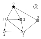
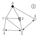
Figure 1: A naive extension of algorithm ${\cal A}_{\mathsf{AF}}$ does not terminate in case of intermittent channel availability. The configuration of round $5$ repeats itself in round $9$.

There is no striking reason for the failure of this naive attempt to fix ${\cal A}_{\mathsf{AF}}$. To analyze the failure we reconsider the proof of termination of the original algorithm ${\cal A}_{\mathsf{AF}}$ in [4]. This paper introduces for a given graph $G$ and a broadcasting node $v_{0}$ the bipartite auxiliary graph ${\cal G}(v_{0})$ and shows that executions of ${\cal A}_{\mathsf{AF}}$ on $G$ and ${\cal G}(v_{0})$ are tightly coupled. ${\cal G}(v_{0})$ is a double cover of $G$ that consists of two copies of $G$, where the cross edges with respect to $v_{0}$ are removed. Each cross edges is replaced by two edges leading from one copy of $G$ to the other. Fig. 2 depicts ${\cal G}(v_{0})$ for the graph shown in Fig. 1 (see Def. 3 in [4] for details).

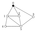
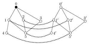
Figure 2: The dashed lines on the left show the cross edges of $G$ ($v_{0}$ is the broadcasting node). The graph ${\cal G}(v_{0})$ is shown on the right, dashed edges are the replacement edges.

An important observation is that ${\cal G}(v_{0})$ is bipartite and that in every round of ${\cal A}_{\mathsf{AF}}$ all nodes that send messages belong to one of the two partitions of nodes. Fig. 3 shows the partitioning of the nodes of ${\cal G}(v_{0})$ for the graph in Fig. 2. An analysis of the execution of Fig. 1 shows that in some rounds, nodes from both partitions forward the message (e.g., in round $3$).

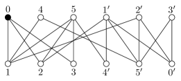
Figure 3: Concurrently forwarding nodes in ${\cal A}_{\mathsf{AF}}$ either all belong the top or bottom row.

4.1 Algorithm ${\cal A}_{\mathsf{AFI}}$

The last observation leads to the following extension of ${\cal A}_{\mathsf{AF}}$ for intermittent availabilities. If a message cannot be forwarded in the current round, it will be postponed until the next available round with the same parity, i.e., if the blocked round is odd (resp. even), the message will be forwarded in the next available odd (resp. even) round. This approach guarantees that as in ${\cal A}_{\mathsf{AF}}$ all nodes that concurrently send messages belong to same of the two node sets. Alg. 2 shows a realization ${\cal A}_{\mathsf{AFI}}$ of this idea. Compared to ${\cal A}_{\mathsf{AF}}$ the new algorithm maintains two sets for the senders of the message in the variable $M$, one for messages that arrive in odd rounds and one for even rounds. The parity is maintained by the Boolean variable parity. The initialization of parity does not need be the same for all nodes. The symbol $\bot$ is used to indicate that no message has arrived in rounds with the specified parity. This is needed to distinguish this situation from the case that a node wants to broadcast a message, in this case $M(\textit{parity})$ is assigned the empty set. If we insert a node $w$ into $M(\textit{parity})$ when $M(\textit{parity})=\bot$ then $M(\textit{parity})=\{w\}$ afterwards. Messages sent in round $i$ are received in round $i+1$. Hence, in round $1$ no message is received.

Initialization

     parity:= true;

     $M(\mathit{true}):=M(\mathit{false}):=\bot$;

Upon receiving message $m$ from $w$:

     $M(\textit{parity}).add(w)$;

if channel is available and $M(\textit{parity})\not=\bot$ then

       forall $u\in N(v)\setminus M(\textit{parity})$ do send($u,m$);

       $M(\textit{parity}):=\bot$;

At the end of each round

     $\textit{parity}:=\neg\textit{parity}$;

function broadcast($m$)

     $M(\textit{parity}):=\emptyset$;

Algorithm 2 Algorithm ${\cal A}_{\mathsf{AFI}}$ distributes a message $m$ in the graph $G$

Fig. 4 shows an execution of algorithm ${\cal A}_{\mathsf{AFI}}$ for the graph of Fig. 1, given that node $v_{2}$ (resp. $v_{3}$) cannot send in rounds $2$ to $4$ (resp. $2$). The execution terminates after round $5$, with no indeterminacy the algorithm would terminate in $4$ rounds (see App. A).

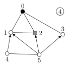
Figure 4: Execution of ${\cal A}_{\mathsf{AFI}}$ for the graph of Fig. 1. Round $1$ is the same as in Fig. 1. In round $6$ node $v_{2}$ does not need to forward the message because, it received messages from all neighbors in odd rounds ($1,3,5$). Whereas $v_{2}$ has to send a message to $v_{0}$ in round $5$ because it only received the message from $v_{1}$ and $v_{5}$ in even rounds $2$ and $4$.

Clearly this extension of ${\cal A}_{\mathsf{AF}}$ is no longer stateless, but because of message buffering no stateless algorithm can handle channel unavailabilities.

4.2 Correctness and Complexity of Algorithm ${\cal A}_{\mathsf{AFI}}$

To formally describe a node’s channel availability for message forwarding the concept of an availability scheme is introduced. Let $A:V\times\mathbb{N}\longrightarrow\{true,false\}$ be a function. Node $v$ can send a message in round $c_{v}$ only if $A(v,c_{v})=true$. $A$ is called an availability scheme for $G$ and $v_{0}$ if the number of pairs $(v,i)\in V\times\mathbb{N}$ with $A(v,i)=\mathit{false}$ is bounded by a constant $c$. Note that this concept is only used in the formal proof. Nodes do not need to have a common round counter. The availability scheme for Fig. 1 is $A(v_{2},2)=A(v_{2},3)=A(v_{2},4)=A(v_{3},2)=\mathit{false}$ and $\mathit{true}$ otherwise. WLOG we always assume that $A(v_{0},1)=true$.

For a given availability scheme $A$ we construct a directed bipartite graph ${\cal B}_{A}(v_{0})$ such that the execution of ${\cal A}_{\mathsf{AFI}}$ on $G$ with respect to $A$ is equivalent to the execution of amnesiac flooding ${\cal A}_{\mathsf{AF}}$ on ${\cal B}_{A}(v_{0})$. The starting point for the construction of ${\cal B}_{A}(v_{0})$ is the double cover ${\cal G}(v_{0})$ of $G$ as defined in the last section. To keep the notation simple we will omit the reference to the originating node $v_{0}$ and refer to the two graphs as ${\cal B}_{A}$ and ${\cal G}$.

First we extend the definition of the availability scheme $A$ to all nodes of ${\cal G}$, i.e., $A:V\cup V^{\prime}\times\mathbb{N}\longrightarrow\{\mathit{true},\mathit{false}\}$. For each node $v^{\prime}\in V^{\prime}$ let $A(v^{\prime},i)=A(v,i)$ for all $i\in\mathbb{N}$. The nodes of ${\cal B}_{A}$ are of two different types: copies of nodes of ${\cal G}$ and so called dummy nodes. We define ${\cal B}_{A}$ inductively, layer by layer. There can be copies of the same node $v$ of ${\cal G}$ on several layers of ${\cal B}_{A}$, but the nodes of a single layer of ${\cal B}_{A}$ are copies of different nodes of ${\cal G}$. Therefore, we do not cause ambiguity when we denote the copies of the nodes by their original names. The construction of ${\cal B}_{A}$ is based on a function originator, that assigns to each node $v$ of ${\cal B}_{A}$ a set of neighbors of $v$ in ${\cal G}$. This function is also defined recursively.

Layer $0$ of ${\cal B}_{A}$ consists of copy of $v_{0}$ with $\textit{originator}(v_{0})=\emptyset$. Layer $1$ consists of copies of the neighbors of $v_{0}$ in ${\cal G}$, these are also the neighbors of $v_{0}$ in $G$. All layer $1$ nodes are successors of $v_{0}$ and the originator of these nodes is $\{v_{0}\}$. Next assume that layers $0$ to $i$ with $i\geq 0$ are already defined including the function originator. We first define the nodes of layer $i+1$ and afterwards the function originator. For each node of layer $i$ we also define the successors. We do this first for nodes which are copies of nodes of ${\cal G}$ and afterwards for dummy nodes.

Let $v$ be a node of layer $i$ that is a copy of a node of ${\cal G}$. If $\textit{originator}(v)=N_{{\cal G}}(v)$ then $v$ has no successor in layer $i+1$. Assume $\textit{originator}(v)\not=N_{{\cal G}}(v)$. First consider the case $A(v,i+1)=\textit{true}$. Let $U=N_{{\cal G}}(v)\setminus\textit{originator}(v)$. For each $u\in U$ we do the following: If layer $i+1$ already contains a copy of $u$ then we make it a successor of $v$. Otherwise, we insert a new copy of $u$ into layer $i+1$ and make it a successor of $v$. If $A(v,i+1)=\textit{false}$ then we create a new dummy node, insert it into layer $i+1$, and make it the single successor of $v$. Finally, let $v$ be a dummy node of layer $i$ and $w$ its single predecessor in layer $i-1$. If layer $i+1$ already contains a copy of $w$ then we make it a successor of $v$. Otherwise, we create a new copy of $w$, insert it into layer $i+1$, and make it the successor of $v$.

To define originator for each node $v$ of layer $i+1$ let $\mathit{pred}(v)$ be the set of predecessors of a node $v$ in $\cal B$. With $\mathit{pred_{d}}(v)$ we denote the dummy nodes in $\mathit{pred}(v)$. Since dummy nodes only have a single predecessor we denote the predecessor in this case also by $\mathit{pred}(v)$. If $v$ is not a dummy node then we define

$$\textit{originator}(v)=\bigcup_{w\in\mathit{pred}_{d}(v)}\!\!\!\!\!\!\!\!\textit{originator}(w)\,\,\ \cup\,\,\,\mathit{pred}(v)\!\setminus\!\mathit{pred}_{d}(v)$$

otherwise $\textit{originator}(v)=\textit{originator}(\textit{pred}(v))$. Note that ${\cal B}_{A}$ is bipartite, since nodes of the same layer are not connected. Fig. 5 shows the graph ${\cal B}_{A}$ for the graph of Fig. 1 and availability scheme $A$. The dummy nodes are labeled $a$ to $d$. We have $\textit{originator}(a)=\textit{originator}(b)=\{v_{0}\}$, $\textit{originator}(c)=\{v_{1}\}$, and $\textit{originator}(d)=\{v_{0},v_{5}\}$. Also, $\textit{originator}(v_{2})=\{v_{0},v_{5},v_{1^{\prime}}\}$ in layer $5$.

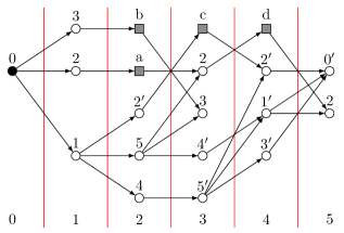
Figure 5: The graph ${\cal B}_{A}$ for the availability scheme $A$ has four dummy nodes.

We orient the edges of ${\cal G}$ by executing a breadth-first search starting in $v_{0}$. The union of the successors and predecessors of a node in ${\cal G}$ are precisely the neighbors of the node in $G$. The next lemma follows from Lemma 5 of [4].

Lemma 2.

Let $v$ be a node of layer $i\geq 0$ of ${\cal G}$. The predecessors of $v$ in ${\cal G}$ are copies of the nodes in $G$ that send in round $i$ of an execution of ${\cal A}_{\mathsf{AF}}$ a message to $v$ and the successors of $v$ in ${\cal G}$ receive a message from $v$ in round $i+1$.

Proof.

Suppose that a node $w$ sends in round $i$ a message to a node $v$. By Lemma 5 of [4] $w$ is a node of layer $i-1$ and either $v$ or $v^{\prime}$ is a successor of $w$ in ${\cal B}$ or $w^{\prime}$ is a node of layer $i-1$ and $v^{\prime}$ is a successor of $w$. Note that in ${\cal B}$ a node of $G$ and its copy cannot be in the same layer. The second statement also follows from this lemma. ∎

Let $A$ be any availability scheme for $G$ and $v_{0}$. Lemma 3 is easy to prove.

Lemma 3.

Let $v$ be a node of ${\cal G}$. For each copy $u$ of $v$ in ${\cal B}_{A}$ we have $N_{{\cal G}(v_{0})}(v)=\textit{originator}(u)\cup\textit{succ}(u)$. If none of the predecessors of $v$ in ${\cal B}$ is a dummy node then $N_{{\cal G}(v_{0})}(v)=\textit{pred}(u)\cup\textit{succ}(u)$.

To illustrate the last lemma we consider the execution from Fig. 4 and the corresponding graph ${\cal B}_{A}$ in Fig. 5. Let $i=4$ and consider node $v_{2}$. The copy of $v_{2}$ on layer $4$ is called $v_{2^{\prime}}$. Fig. 5 shows that $\textit{originator}(v_{2})=\{v_{5},v_{1}\}$. From Fig. 4 we see that node $v_{2}$ receives a message from node $v_{1}$, i.e., $v_{1}\in v_{2}.M(\textit{parity})$. Since $A(v_{2},3)=\mathit{false}$ node $v_{2}$ could not send a message in round $3$. Hence the sender $v_{1}$ of the message received in round $3$ is still in $v_{2}.M(\textit{parity})$. This yields $v_{2}.M(\textit{parity})=\{v_{5},v_{1}\}$, since $A(v_{2},1)=\mathit{true}$.

For an availability scheme $A$ and $k\geq 0$ we define a new availability scheme $A_{k}$ as follows. We consider the nodes of ${\cal B}_{A}$ in any arbitrary but fixed order and define a total order on the set of pairs $(v,i)\in V\times\mathbb{N}$ with $A(v,i)=\mathit{false}$ as follows: $(v,i)<(w,j)$ if and only if $i<j$ or $i=j$ and $v<w$. Then we define $A_{k}(v,i)=\mathit{false}$ for all but the first $k$ pairs $(v,i)$, i.e., $A_{k}$ has value $\mathit{false}$ for exactly $k$ pairs $(v,i)$. Note that there exists $c>0$ such that $A=A_{c}$.

Lemma 4.

There is a one-to-one mapping between the edges of ${\cal G}$ and those edges of ${\cal B}_{A}$ that are not incident to a dummy node.

Proof.

It suffices to prove that the lemma holds for each $A_{k}$ with $k\geq 0$. The proof is by induction on $k$. If $k=0$ then the result is trivially true since ${\cal B}_{A_{0}}={\cal G}$. Assume the theorem is true for $k\geq 1$. Consider the graph ${\cal B}_{A_{k-1}}$. Let $(v,i)$ be the $k^{th}$ pair with $A(v,i)=\mathit{false}$. If layer $i-1$ of ${\cal B}_{A_{k-1}}$ contains no copy of $v$ then ${\cal B}_{A_{k-1}}={\cal B}_{A_{k}}$ and we are done. Suppose there exists a copy of $v$ on layer $i-1$ of ${\cal B}_{A_{k-1}}$. We inductively define two sequences of sets $X_{j}$, $\mathchoice{\hbox to0.0pt{\hbox to9.06943pt{\hfill$\overline{\vrule width=0.0pt,height=6.83331pt\kern 7.50002pt}$}\hss}\hbox{\set@color$\displaystyle X$}}{\hbox to0.0pt{\hbox to9.06943pt{\hfill$\overline{\vrule width=0.0pt,height=6.83331pt\kern 7.50002pt}$}\hss}\hbox{\set@color$\textstyle X$}}{\hbox to0.0pt{\hbox to6.3486pt{\hfill$\overline{\vrule width=0.0pt,height=4.78333pt\kern 5.25pt}$}\hss}\hbox{\set@color$\scriptstyle X$}}{\hbox to0.0pt{\hbox to4.53471pt{\hfill$\overline{\vrule width=0.0pt,height=3.41666pt\kern 3.75pt}$}\hss}\hbox{\set@color$\scriptscriptstyle X$}}_{j}$ ($j\geq 1$) of nodes of ${\cal B}_{A_{k-1}}$ (see Fig. 6). Nodes of $X_{j}$, $\mathchoice{\hbox to0.0pt{\hbox to9.06943pt{\hfill$\overline{\vrule width=0.0pt,height=6.83331pt\kern 7.50002pt}$}\hss}\hbox{\set@color$\displaystyle X$}}{\hbox to0.0pt{\hbox to9.06943pt{\hfill$\overline{\vrule width=0.0pt,height=6.83331pt\kern 7.50002pt}$}\hss}\hbox{\set@color$\textstyle X$}}{\hbox to0.0pt{\hbox to6.3486pt{\hfill$\overline{\vrule width=0.0pt,height=4.78333pt\kern 5.25pt}$}\hss}\hbox{\set@color$\scriptstyle X$}}{\hbox to0.0pt{\hbox to4.53471pt{\hfill$\overline{\vrule width=0.0pt,height=3.41666pt\kern 3.75pt}$}\hss}\hbox{\set@color$\scriptscriptstyle X$}}_{j}$ are in layer $i-1+j$ of ${\cal B}_{A_{k-1}}$. $X_{1}$ is the set of nodes of layer $i$ that have $v$ as the single predecessor in layer $i-1$ and $\mathchoice{\hbox to0.0pt{\hbox to9.06943pt{\hfill$\overline{\vrule width=0.0pt,height=6.83331pt\kern 7.50002pt}$}\hss}\hbox{\set@color$\displaystyle X$}}{\hbox to0.0pt{\hbox to9.06943pt{\hfill$\overline{\vrule width=0.0pt,height=6.83331pt\kern 7.50002pt}$}\hss}\hbox{\set@color$\textstyle X$}}{\hbox to0.0pt{\hbox to6.3486pt{\hfill$\overline{\vrule width=0.0pt,height=4.78333pt\kern 5.25pt}$}\hss}\hbox{\set@color$\scriptstyle X$}}{\hbox to0.0pt{\hbox to4.53471pt{\hfill$\overline{\vrule width=0.0pt,height=3.41666pt\kern 3.75pt}$}\hss}\hbox{\set@color$\scriptscriptstyle X$}}_{1}=\mathit{succ}(v)\setminus X_{1}$, where $\mathit{succ}(v)$ denotes the successors in ${\cal B}_{A_{k-1}}$. Thus, each node in $\mathchoice{\hbox to0.0pt{\hbox to9.06943pt{\hfill$\overline{\vrule width=0.0pt,height=6.83331pt\kern 7.50002pt}$}\hss}\hbox{\set@color$\displaystyle X$}}{\hbox to0.0pt{\hbox to9.06943pt{\hfill$\overline{\vrule width=0.0pt,height=6.83331pt\kern 7.50002pt}$}\hss}\hbox{\set@color$\textstyle X$}}{\hbox to0.0pt{\hbox to6.3486pt{\hfill$\overline{\vrule width=0.0pt,height=4.78333pt\kern 5.25pt}$}\hss}\hbox{\set@color$\scriptstyle X$}}{\hbox to0.0pt{\hbox to4.53471pt{\hfill$\overline{\vrule width=0.0pt,height=3.41666pt\kern 3.75pt}$}\hss}\hbox{\set@color$\scriptscriptstyle X$}}_{1}$ has besides $v$ another predecessor in layer $i-1$. Suppose we already defined $X_{j-1},\mathchoice{\hbox to0.0pt{\hbox to9.06943pt{\hfill$\overline{\vrule width=0.0pt,height=6.83331pt\kern 7.50002pt}$}\hss}\hbox{\set@color$\displaystyle X$}}{\hbox to0.0pt{\hbox to9.06943pt{\hfill$\overline{\vrule width=0.0pt,height=6.83331pt\kern 7.50002pt}$}\hss}\hbox{\set@color$\textstyle X$}}{\hbox to0.0pt{\hbox to6.3486pt{\hfill$\overline{\vrule width=0.0pt,height=4.78333pt\kern 5.25pt}$}\hss}\hbox{\set@color$\scriptstyle X$}}{\hbox to0.0pt{\hbox to4.53471pt{\hfill$\overline{\vrule width=0.0pt,height=3.41666pt\kern 3.75pt}$}\hss}\hbox{\set@color$\scriptscriptstyle X$}}_{j-1}$. Then $X_{j}$ is the set of nodes of layer $i-1+j$ that have only predecessors in $X_{j-1}$, i.e., $\mathit{pred}(X_{j})\subseteq X_{j-1}$. $\mathchoice{\hbox to0.0pt{\hbox to9.06943pt{\hfill$\overline{\vrule width=0.0pt,height=6.83331pt\kern 7.50002pt}$}\hss}\hbox{\set@color$\displaystyle X$}}{\hbox to0.0pt{\hbox to9.06943pt{\hfill$\overline{\vrule width=0.0pt,height=6.83331pt\kern 7.50002pt}$}\hss}\hbox{\set@color$\textstyle X$}}{\hbox to0.0pt{\hbox to6.3486pt{\hfill$\overline{\vrule width=0.0pt,height=4.78333pt\kern 5.25pt}$}\hss}\hbox{\set@color$\scriptstyle X$}}{\hbox to0.0pt{\hbox to4.53471pt{\hfill$\overline{\vrule width=0.0pt,height=3.41666pt\kern 3.75pt}$}\hss}\hbox{\set@color$\scriptscriptstyle X$}}_{j}$ consists of those nodes of layer $i-1+j$ that have predecessors in $X_{j-1}$ and in $\mathchoice{\hbox to0.0pt{\hbox to9.06943pt{\hfill$\overline{\vrule width=0.0pt,height=6.83331pt\kern 7.50002pt}$}\hss}\hbox{\set@color$\displaystyle X$}}{\hbox to0.0pt{\hbox to9.06943pt{\hfill$\overline{\vrule width=0.0pt,height=6.83331pt\kern 7.50002pt}$}\hss}\hbox{\set@color$\textstyle X$}}{\hbox to0.0pt{\hbox to6.3486pt{\hfill$\overline{\vrule width=0.0pt,height=4.78333pt\kern 5.25pt}$}\hss}\hbox{\set@color$\scriptstyle X$}}{\hbox to0.0pt{\hbox to4.53471pt{\hfill$\overline{\vrule width=0.0pt,height=3.41666pt\kern 3.75pt}$}\hss}\hbox{\set@color$\scriptscriptstyle X$}}_{j-1}$, i.e., for each $w\in\mathchoice{\hbox to0.0pt{\hbox to9.06943pt{\hfill$\overline{\vrule width=0.0pt,height=6.83331pt\kern 7.50002pt}$}\hss}\hbox{\set@color$\displaystyle X$}}{\hbox to0.0pt{\hbox to9.06943pt{\hfill$\overline{\vrule width=0.0pt,height=6.83331pt\kern 7.50002pt}$}\hss}\hbox{\set@color$\textstyle X$}}{\hbox to0.0pt{\hbox to6.3486pt{\hfill$\overline{\vrule width=0.0pt,height=4.78333pt\kern 5.25pt}$}\hss}\hbox{\set@color$\scriptstyle X$}}{\hbox to0.0pt{\hbox to4.53471pt{\hfill$\overline{\vrule width=0.0pt,height=3.41666pt\kern 3.75pt}$}\hss}\hbox{\set@color$\scriptscriptstyle X$}}_{j}$ we have $pred(w)\cap X_{j-1}\not=\emptyset$ and $pred(w)\cap\mathchoice{\hbox to0.0pt{\hbox to9.06943pt{\hfill$\overline{\vrule width=0.0pt,height=6.83331pt\kern 7.50002pt}$}\hss}\hbox{\set@color$\displaystyle X$}}{\hbox to0.0pt{\hbox to9.06943pt{\hfill$\overline{\vrule width=0.0pt,height=6.83331pt\kern 7.50002pt}$}\hss}\hbox{\set@color$\textstyle X$}}{\hbox to0.0pt{\hbox to6.3486pt{\hfill$\overline{\vrule width=0.0pt,height=4.78333pt\kern 5.25pt}$}\hss}\hbox{\set@color$\scriptstyle X$}}{\hbox to0.0pt{\hbox to4.53471pt{\hfill$\overline{\vrule width=0.0pt,height=3.41666pt\kern 3.75pt}$}\hss}\hbox{\set@color$\scriptscriptstyle X$}}_{j-1}\not=\emptyset$. Hence, $\mathit{succ}(X_{j-1})=X_{j}\,\dot{\cup}\,\mathchoice{\hbox to0.0pt{\hbox to9.06943pt{\hfill$\overline{\vrule width=0.0pt,height=6.83331pt\kern 7.50002pt}$}\hss}\hbox{\set@color$\displaystyle X$}}{\hbox to0.0pt{\hbox to9.06943pt{\hfill$\overline{\vrule width=0.0pt,height=6.83331pt\kern 7.50002pt}$}\hss}\hbox{\set@color$\textstyle X$}}{\hbox to0.0pt{\hbox to6.3486pt{\hfill$\overline{\vrule width=0.0pt,height=4.78333pt\kern 5.25pt}$}\hss}\hbox{\set@color$\scriptstyle X$}}{\hbox to0.0pt{\hbox to4.53471pt{\hfill$\overline{\vrule width=0.0pt,height=3.41666pt\kern 3.75pt}$}\hss}\hbox{\set@color$\scriptscriptstyle X$}}_{j}$. Note that none of the nodes of $X_{j}$, $\mathchoice{\hbox to0.0pt{\hbox to9.06943pt{\hfill$\overline{\vrule width=0.0pt,height=6.83331pt\kern 7.50002pt}$}\hss}\hbox{\set@color$\displaystyle X$}}{\hbox to0.0pt{\hbox to9.06943pt{\hfill$\overline{\vrule width=0.0pt,height=6.83331pt\kern 7.50002pt}$}\hss}\hbox{\set@color$\textstyle X$}}{\hbox to0.0pt{\hbox to6.3486pt{\hfill$\overline{\vrule width=0.0pt,height=4.78333pt\kern 5.25pt}$}\hss}\hbox{\set@color$\scriptstyle X$}}{\hbox to0.0pt{\hbox to4.53471pt{\hfill$\overline{\vrule width=0.0pt,height=3.41666pt\kern 3.75pt}$}\hss}\hbox{\set@color$\scriptscriptstyle X$}}_{j}$ are dummy nodes, therefore $N_{{\cal G}}(u)=\textit{pred}(u)\cup\textit{succ}(u)$ for each $u\in X_{j}\cup\mathchoice{\hbox to0.0pt{\hbox to9.06943pt{\hfill$\overline{\vrule width=0.0pt,height=6.83331pt\kern 7.50002pt}$}\hss}\hbox{\set@color$\displaystyle X$}}{\hbox to0.0pt{\hbox to9.06943pt{\hfill$\overline{\vrule width=0.0pt,height=6.83331pt\kern 7.50002pt}$}\hss}\hbox{\set@color$\textstyle X$}}{\hbox to0.0pt{\hbox to6.3486pt{\hfill$\overline{\vrule width=0.0pt,height=4.78333pt\kern 5.25pt}$}\hss}\hbox{\set@color$\scriptstyle X$}}{\hbox to0.0pt{\hbox to4.53471pt{\hfill$\overline{\vrule width=0.0pt,height=3.41666pt\kern 3.75pt}$}\hss}\hbox{\set@color$\scriptscriptstyle X$}}_{j}$ by Lemma 3. Since the theorem is true for $A_{k-1}$, there exist $t$ such that $X_{t}=\emptyset$. Note that $X_{j}\not=\emptyset$ for $j=1,\ldots t-1$ while $\mathchoice{\hbox to0.0pt{\hbox to9.06943pt{\hfill$\overline{\vrule width=0.0pt,height=6.83331pt\kern 7.50002pt}$}\hss}\hbox{\set@color$\displaystyle X$}}{\hbox to0.0pt{\hbox to9.06943pt{\hfill$\overline{\vrule width=0.0pt,height=6.83331pt\kern 7.50002pt}$}\hss}\hbox{\set@color$\textstyle X$}}{\hbox to0.0pt{\hbox to6.3486pt{\hfill$\overline{\vrule width=0.0pt,height=4.78333pt\kern 5.25pt}$}\hss}\hbox{\set@color$\scriptstyle X$}}{\hbox to0.0pt{\hbox to4.53471pt{\hfill$\overline{\vrule width=0.0pt,height=3.41666pt\kern 3.75pt}$}\hss}\hbox{\set@color$\scriptscriptstyle X$}}_{j}$ can be empty for any $j$.

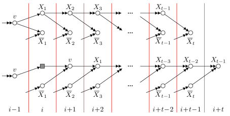
Figure 6: The top row illustrates the definition of $X_{j}$ and $\mathchoice{\hbox to0.0pt{\hbox to9.06943pt{\hfill$\overline{\vrule width=0.0pt,height=6.83331pt\kern 7.50002pt}$}\hss}\hbox{\set@color$\displaystyle X$}}{\hbox to0.0pt{\hbox to9.06943pt{\hfill$\overline{\vrule width=0.0pt,height=6.83331pt\kern 7.50002pt}$}\hss}\hbox{\set@color$\textstyle X$}}{\hbox to0.0pt{\hbox to6.3486pt{\hfill$\overline{\vrule width=0.0pt,height=4.78333pt\kern 5.25pt}$}\hss}\hbox{\set@color$\scriptstyle X$}}{\hbox to0.0pt{\hbox to4.53471pt{\hfill$\overline{\vrule width=0.0pt,height=3.41666pt\kern 3.75pt}$}\hss}\hbox{\set@color$\scriptscriptstyle X$}}_{j}$ for ${\cal B}_{A_{k-1}}$. The lower row displays the changes in ${\cal B}_{A_{k}}$ compared with ${\cal B}_{A_{k-1}}$. The last row indicates the number of the layer. The symbol indicates that there can be several edges.

Next, we show how ${\cal B}_{A_{k}}$ can be derived from ${\cal B}_{A_{k-1}}$. The two graphs coincide completely in the first $i-1$ layers. In subsequent layers nodes that are not reachable from $v$ in layer $i-1$ also are identical. The single successor of $v$ in layer $i$ is the dummy node. This node itself has as successor a copy of $v$ on layer $i+1$. Clearly this copy of $v$ is also the successor of all nodes in $\mathchoice{\hbox to0.0pt{\hbox to9.06943pt{\hfill$\overline{\vrule width=0.0pt,height=6.83331pt\kern 7.50002pt}$}\hss}\hbox{\set@color$\displaystyle X$}}{\hbox to0.0pt{\hbox to9.06943pt{\hfill$\overline{\vrule width=0.0pt,height=6.83331pt\kern 7.50002pt}$}\hss}\hbox{\set@color$\textstyle X$}}{\hbox to0.0pt{\hbox to6.3486pt{\hfill$\overline{\vrule width=0.0pt,height=4.78333pt\kern 5.25pt}$}\hss}\hbox{\set@color$\scriptstyle X$}}{\hbox to0.0pt{\hbox to4.53471pt{\hfill$\overline{\vrule width=0.0pt,height=3.41666pt\kern 3.75pt}$}\hss}\hbox{\set@color$\scriptscriptstyle X$}}_{1}$ in layer $i$. The successors of the copy of $v$ on layer $i+1$ are copies of the nodes of set $X_{1}$. Nodes in $\mathchoice{\hbox to0.0pt{\hbox to9.06943pt{\hfill$\overline{\vrule width=0.0pt,height=6.83331pt\kern 7.50002pt}$}\hss}\hbox{\set@color$\displaystyle X$}}{\hbox to0.0pt{\hbox to9.06943pt{\hfill$\overline{\vrule width=0.0pt,height=6.83331pt\kern 7.50002pt}$}\hss}\hbox{\set@color$\textstyle X$}}{\hbox to0.0pt{\hbox to6.3486pt{\hfill$\overline{\vrule width=0.0pt,height=4.78333pt\kern 5.25pt}$}\hss}\hbox{\set@color$\scriptstyle X$}}{\hbox to0.0pt{\hbox to4.53471pt{\hfill$\overline{\vrule width=0.0pt,height=3.41666pt\kern 3.75pt}$}\hss}\hbox{\set@color$\scriptscriptstyle X$}}_{2}$ on layer $i+1$ are the predecessors of nodes in $X_{1}$. All these statements are an immediate consequence of Lemma 3. Similarly it follows that each layer $i-1+j$ for $j\geq 3$ contains copies of the nodes of set $X_{j-2}$. Their predecessors are copies of the nodes in $X_{j-3}$ and $\mathchoice{\hbox to0.0pt{\hbox to9.06943pt{\hfill$\overline{\vrule width=0.0pt,height=6.83331pt\kern 7.50002pt}$}\hss}\hbox{\set@color$\displaystyle X$}}{\hbox to0.0pt{\hbox to9.06943pt{\hfill$\overline{\vrule width=0.0pt,height=6.83331pt\kern 7.50002pt}$}\hss}\hbox{\set@color$\textstyle X$}}{\hbox to0.0pt{\hbox to6.3486pt{\hfill$\overline{\vrule width=0.0pt,height=4.78333pt\kern 5.25pt}$}\hss}\hbox{\set@color$\scriptstyle X$}}{\hbox to0.0pt{\hbox to4.53471pt{\hfill$\overline{\vrule width=0.0pt,height=3.41666pt\kern 3.75pt}$}\hss}\hbox{\set@color$\scriptscriptstyle X$}}_{j-1}$.

Thus, in $B_{A_{k}}$ some edges from $B_{A_{k-1}}$ are reversed: The orientation of edges from $X_{j}$ to $\mathchoice{\hbox to0.0pt{\hbox to9.06943pt{\hfill$\overline{\vrule width=0.0pt,height=6.83331pt\kern 7.50002pt}$}\hss}\hbox{\set@color$\displaystyle X$}}{\hbox to0.0pt{\hbox to9.06943pt{\hfill$\overline{\vrule width=0.0pt,height=6.83331pt\kern 7.50002pt}$}\hss}\hbox{\set@color$\textstyle X$}}{\hbox to0.0pt{\hbox to6.3486pt{\hfill$\overline{\vrule width=0.0pt,height=4.78333pt\kern 5.25pt}$}\hss}\hbox{\set@color$\scriptstyle X$}}{\hbox to0.0pt{\hbox to4.53471pt{\hfill$\overline{\vrule width=0.0pt,height=3.41666pt\kern 3.75pt}$}\hss}\hbox{\set@color$\scriptscriptstyle X$}}_{j+1}$ and from $v$ to $\mathchoice{\hbox to0.0pt{\hbox to9.06943pt{\hfill$\overline{\vrule width=0.0pt,height=6.83331pt\kern 7.50002pt}$}\hss}\hbox{\set@color$\displaystyle X$}}{\hbox to0.0pt{\hbox to9.06943pt{\hfill$\overline{\vrule width=0.0pt,height=6.83331pt\kern 7.50002pt}$}\hss}\hbox{\set@color$\textstyle X$}}{\hbox to0.0pt{\hbox to6.3486pt{\hfill$\overline{\vrule width=0.0pt,height=4.78333pt\kern 5.25pt}$}\hss}\hbox{\set@color$\scriptstyle X$}}{\hbox to0.0pt{\hbox to4.53471pt{\hfill$\overline{\vrule width=0.0pt,height=3.41666pt\kern 3.75pt}$}\hss}\hbox{\set@color$\scriptscriptstyle X$}}_{1}$ is reversed. This analysis also shows that $B_{A_{k}}$ only has two additional edges, those adjacent to the new dummy node. In the worst case, $B_{A_{k}}$ consists of two more layers compared to $B_{A_{k-1}}$. ∎

To ease the formulation of the next lemma we introduce another definition. Let $u$ be a node of $G$. For a copy of $u$ in layer $i$ of ${\cal B}_{A}$ we denote the originators in ${\cal B}_{A}$ of this copy of $v$ by $\textit{originator}^{i}(v)$. Furthermore, the set $M(\textit{parity})$ of node $u$ immediately before checking channel availability in round $i$ during an execution of ${\cal A}_{\mathsf{AFI}}$ on $G$ is denoted by $v.M^{i}(\textit{parity})$.

Lemma 5.

Let $u$ be a non-dummy node of layer $i$ of ${\cal B}_{A}$. Then $u.M^{i}(\textit{parity})=\textit{originator}^{i}(u)$.

Proof.

We use the notation introduced in the proof of Lemma 4. As before we prove by induction on $k$ that the lemma holds for $A_{k}$. If $k=0$ then the result holds by Lemma 2 since ${\cal B}_{A_{0}}={\cal G}$. Assume the lemma is true for $k\geq 1$. We consider the graph ${\cal B}_{A_{k-1}}$. Let $(v,i)$ be the $k^{th}$ pair with $A(v,i)=\mathit{false}$. If in layer $i-1$ of ${\cal B}_{A_{k-1}}$ there exists no copy of $v$ then ${\cal B}_{A_{k-1}}={\cal B}_{A_{k}}$ and we are done. Suppose there exists a copy of $v$ on layer $i-1$ of ${\cal B}_{A_{k-1}}$. From Fig. 6 we see that we only have to consider the cases $u=v$, $u\in X_{j}$, and $u\in\mathchoice{\hbox to0.0pt{\hbox to9.06943pt{\hfill$\overline{\vrule width=0.0pt,height=6.83331pt\kern 7.50002pt}$}\hss}\hbox{\set@color$\displaystyle X$}}{\hbox to0.0pt{\hbox to9.06943pt{\hfill$\overline{\vrule width=0.0pt,height=6.83331pt\kern 7.50002pt}$}\hss}\hbox{\set@color$\textstyle X$}}{\hbox to0.0pt{\hbox to6.3486pt{\hfill$\overline{\vrule width=0.0pt,height=4.78333pt\kern 5.25pt}$}\hss}\hbox{\set@color$\scriptstyle X$}}{\hbox to0.0pt{\hbox to4.53471pt{\hfill$\overline{\vrule width=0.0pt,height=3.41666pt\kern 3.75pt}$}\hss}\hbox{\set@color$\scriptscriptstyle X$}}_{j}$. Remember that there are no dummy nodes in $X_{j}$, $\mathchoice{\hbox to0.0pt{\hbox to9.06943pt{\hfill$\overline{\vrule width=0.0pt,height=6.83331pt\kern 7.50002pt}$}\hss}\hbox{\set@color$\displaystyle X$}}{\hbox to0.0pt{\hbox to9.06943pt{\hfill$\overline{\vrule width=0.0pt,height=6.83331pt\kern 7.50002pt}$}\hss}\hbox{\set@color$\textstyle X$}}{\hbox to0.0pt{\hbox to6.3486pt{\hfill$\overline{\vrule width=0.0pt,height=4.78333pt\kern 5.25pt}$}\hss}\hbox{\set@color$\scriptstyle X$}}{\hbox to0.0pt{\hbox to4.53471pt{\hfill$\overline{\vrule width=0.0pt,height=3.41666pt\kern 3.75pt}$}\hss}\hbox{\set@color$\scriptscriptstyle X$}}_{j}$.

First consider the case that $u$ is the copy of $v$ in layer $i+1$ in ${\cal B}_{A_{k}}$ (see Fig. 6). In round $i+1$ in ${\cal B}_{A_{k}}$ the nodes in $\mathchoice{\hbox to0.0pt{\hbox to9.06943pt{\hfill$\overline{\vrule width=0.0pt,height=6.83331pt\kern 7.50002pt}$}\hss}\hbox{\set@color$\displaystyle X$}}{\hbox to0.0pt{\hbox to9.06943pt{\hfill$\overline{\vrule width=0.0pt,height=6.83331pt\kern 7.50002pt}$}\hss}\hbox{\set@color$\textstyle X$}}{\hbox to0.0pt{\hbox to6.3486pt{\hfill$\overline{\vrule width=0.0pt,height=4.78333pt\kern 5.25pt}$}\hss}\hbox{\set@color$\scriptstyle X$}}{\hbox to0.0pt{\hbox to4.53471pt{\hfill$\overline{\vrule width=0.0pt,height=3.41666pt\kern 3.75pt}$}\hss}\hbox{\set@color$\scriptscriptstyle X$}}_{1}$ do not receive the message from $v$ because $A(v,i)=\mathit{false}$. Since each node in $\mathchoice{\hbox to0.0pt{\hbox to9.06943pt{\hfill$\overline{\vrule width=0.0pt,height=6.83331pt\kern 7.50002pt}$}\hss}\hbox{\set@color$\displaystyle X$}}{\hbox to0.0pt{\hbox to9.06943pt{\hfill$\overline{\vrule width=0.0pt,height=6.83331pt\kern 7.50002pt}$}\hss}\hbox{\set@color$\textstyle X$}}{\hbox to0.0pt{\hbox to6.3486pt{\hfill$\overline{\vrule width=0.0pt,height=4.78333pt\kern 5.25pt}$}\hss}\hbox{\set@color$\scriptstyle X$}}{\hbox to0.0pt{\hbox to4.53471pt{\hfill$\overline{\vrule width=0.0pt,height=3.41666pt\kern 3.75pt}$}\hss}\hbox{\set@color$\scriptscriptstyle X$}}_{1}$ still receives the message from another node, each of them must forward the message in round $i$ to $v$. Hence, $v.M^{i+1}(\textit{parity})=v.M^{i-1}(\textit{parity})\cup\mathchoice{\hbox to0.0pt{\hbox to9.06943pt{\hfill$\overline{\vrule width=0.0pt,height=6.83331pt\kern 7.50002pt}$}\hss}\hbox{\set@color$\displaystyle X$}}{\hbox to0.0pt{\hbox to9.06943pt{\hfill$\overline{\vrule width=0.0pt,height=6.83331pt\kern 7.50002pt}$}\hss}\hbox{\set@color$\textstyle X$}}{\hbox to0.0pt{\hbox to6.3486pt{\hfill$\overline{\vrule width=0.0pt,height=4.78333pt\kern 5.25pt}$}\hss}\hbox{\set@color$\scriptstyle X$}}{\hbox to0.0pt{\hbox to4.53471pt{\hfill$\overline{\vrule width=0.0pt,height=3.41666pt\kern 3.75pt}$}\hss}\hbox{\set@color$\scriptscriptstyle X$}}_{1}$. On the other hand $\textit{originator}^{i+1}(v)=\textit{originator}^{i-1}(v)\cup\mathchoice{\hbox to0.0pt{\hbox to9.06943pt{\hfill$\overline{\vrule width=0.0pt,height=6.83331pt\kern 7.50002pt}$}\hss}\hbox{\set@color$\displaystyle X$}}{\hbox to0.0pt{\hbox to9.06943pt{\hfill$\overline{\vrule width=0.0pt,height=6.83331pt\kern 7.50002pt}$}\hss}\hbox{\set@color$\textstyle X$}}{\hbox to0.0pt{\hbox to6.3486pt{\hfill$\overline{\vrule width=0.0pt,height=4.78333pt\kern 5.25pt}$}\hss}\hbox{\set@color$\scriptstyle X$}}{\hbox to0.0pt{\hbox to4.53471pt{\hfill$\overline{\vrule width=0.0pt,height=3.41666pt\kern 3.75pt}$}\hss}\hbox{\set@color$\scriptscriptstyle X$}}_{1}$. By induction $\textit{originator}^{i-1}(v)=v.M^{i-1}(\textit{parity})$.

Next consider the case $u\in X_{1}$. Then $u$ is on layer $i+2$ of ${\cal B}_{k}$. Since in ${\cal B}_{A_{k-1}}$ each node in $X_{1}$ receives in round $i$ only the message from $v$, node $v$ sends the message to each node in $X_{1}$ in round $i+1$. Furthermore, since for ${\cal B}_{A_{k-1}}$ each node in $\mathchoice{\hbox to0.0pt{\hbox to9.06943pt{\hfill$\overline{\vrule width=0.0pt,height=6.83331pt\kern 7.50002pt}$}\hss}\hbox{\set@color$\displaystyle X$}}{\hbox to0.0pt{\hbox to9.06943pt{\hfill$\overline{\vrule width=0.0pt,height=6.83331pt\kern 7.50002pt}$}\hss}\hbox{\set@color$\textstyle X$}}{\hbox to0.0pt{\hbox to6.3486pt{\hfill$\overline{\vrule width=0.0pt,height=4.78333pt\kern 5.25pt}$}\hss}\hbox{\set@color$\scriptstyle X$}}{\hbox to0.0pt{\hbox to4.53471pt{\hfill$\overline{\vrule width=0.0pt,height=3.41666pt\kern 3.75pt}$}\hss}\hbox{\set@color$\scriptscriptstyle X$}}_{2}$ received in round $i+1$ a message from a node in $X_{1}$, each node of $\mathchoice{\hbox to0.0pt{\hbox to9.06943pt{\hfill$\overline{\vrule width=0.0pt,height=6.83331pt\kern 7.50002pt}$}\hss}\hbox{\set@color$\displaystyle X$}}{\hbox to0.0pt{\hbox to9.06943pt{\hfill$\overline{\vrule width=0.0pt,height=6.83331pt\kern 7.50002pt}$}\hss}\hbox{\set@color$\textstyle X$}}{\hbox to0.0pt{\hbox to6.3486pt{\hfill$\overline{\vrule width=0.0pt,height=4.78333pt\kern 5.25pt}$}\hss}\hbox{\set@color$\scriptstyle X$}}{\hbox to0.0pt{\hbox to4.53471pt{\hfill$\overline{\vrule width=0.0pt,height=3.41666pt\kern 3.75pt}$}\hss}\hbox{\set@color$\scriptscriptstyle X$}}_{2}$ sends ${\cal B}_{A_{k}}$ the message to at least one node of $X_{1}$. In particular node $u$ receives in round $i+2$ the message from its predecessors in $\mathchoice{\hbox to0.0pt{\hbox to9.06943pt{\hfill$\overline{\vrule width=0.0pt,height=6.83331pt\kern 7.50002pt}$}\hss}\hbox{\set@color$\displaystyle X$}}{\hbox to0.0pt{\hbox to9.06943pt{\hfill$\overline{\vrule width=0.0pt,height=6.83331pt\kern 7.50002pt}$}\hss}\hbox{\set@color$\textstyle X$}}{\hbox to0.0pt{\hbox to6.3486pt{\hfill$\overline{\vrule width=0.0pt,height=4.78333pt\kern 5.25pt}$}\hss}\hbox{\set@color$\scriptstyle X$}}{\hbox to0.0pt{\hbox to4.53471pt{\hfill$\overline{\vrule width=0.0pt,height=3.41666pt\kern 3.75pt}$}\hss}\hbox{\set@color$\scriptscriptstyle X$}}_{2}$ for ${\cal B}_{A_{k}}$. Clearly, $u$ does not receive the message from any other node. Thus, $u.M^{i+2}(\textit{parity})=\textit{originator}^{i+2}(u)$. The cases $u\in X_{j}$ with $j>1$ and $u\in\mathchoice{\hbox to0.0pt{\hbox to9.06943pt{\hfill$\overline{\vrule width=0.0pt,height=6.83331pt\kern 7.50002pt}$}\hss}\hbox{\set@color$\displaystyle X$}}{\hbox to0.0pt{\hbox to9.06943pt{\hfill$\overline{\vrule width=0.0pt,height=6.83331pt\kern 7.50002pt}$}\hss}\hbox{\set@color$\textstyle X$}}{\hbox to0.0pt{\hbox to6.3486pt{\hfill$\overline{\vrule width=0.0pt,height=4.78333pt\kern 5.25pt}$}\hss}\hbox{\set@color$\scriptstyle X$}}{\hbox to0.0pt{\hbox to4.53471pt{\hfill$\overline{\vrule width=0.0pt,height=3.41666pt\kern 3.75pt}$}\hss}\hbox{\set@color$\scriptscriptstyle X$}}_{j}$ with $j\geq 1$ can be proved similarly. ∎

Lemma 6.

During round $i$ of an executing of ${\cal A}_{\mathsf{AFI}}$ on $G$ a node $v$ sends the message to a neighbor $w$ if and only if the copy of $v$ in layer $i-1$ of ${\cal B}_{A}$ is the predecessor of a copy of $w$ in layer $i$ of ${\cal B}_{A}$.

Proof.

If during the execution of ${\cal A}_{\mathsf{AFI}}$ node $v$ sends messages in round $i$ to $w$ then $A(v,i)=\mathit{true}$ and $N(v)\not=v.M(\textit{parity})$. By the Lemma 5 we have $w\in N(v)\setminus\textit{originator}(v)$. Thus, by construction $w$ is a successor of $v$ in ${\cal B}_{A}$. Conversely, if $w$ is successor of $v$ in ${\cal B}_{A}$ then $A(v,i)=\mathit{true}$ and $v\in N(v)\setminus\textit{originator}(v)$. Again Lemma 5 gives the desired result. ∎

The last lemma implies that executing ${\cal A}_{\mathsf{AFI}}$ on $G$ is equivalent to executing ${\cal A}_{\mathsf{AF}}$ on ${\cal B}_{A}$. The reason is that ${\cal B}_{A}$ is bipartite and executing ${\cal A}_{\mathsf{AF}}$ on a bipartite graph starting at the root is equivalent to synchronous flooding the bipartite graph. This is formulated in the following theorem.

Theorem 7.

Let $G$ be a graph $G$ and $A$ an availability scheme for $G$. Let $f={\left\lvert\{(v,i)\;|\;A(v,i)=\mathit{false}\}\right\rvert}$. Algorithm ${\cal A}_{\mathsf{AFI}}$ delivers a broadcasted message (resp. terminates) after at most $Diam(G)+2f$ (resp. $2Diam(G)+2f+1$) rounds. If $G$ is bipartite each message is forwarded ${\left\lvert E\right\rvert}$ times, otherwise $2{\left\lvert E\right\rvert}$ times.

Proof.

Lemma 6 implies that ${\cal A}_{\mathsf{AFI}}$ terminates after $d$ rounds where $d$ is the height of ${\cal B}_{A}$. The proof of Lemma 4 shows that each pair $(v,i)$ with $A(v,i)=\mathit{false}$ increases the depth by at most $2$. By Thm. 1 of [4] the depth of ${\cal G}$ is at most $2Diam(G)+1$. By Lemma 4 and Lemma 5 ${\cal A}_{\mathsf{AFI}}$ sends $2{\left\lvert E\right\rvert}$ messages. ∎

5 Multi-Source Broadcasts

A variant of broadcasting is multi-source broadcasting, where several nodes invoke a broadcast of the same message, i.e., with the same message id, possibly in different rounds. This problem is motivated by disaster monitoring: A distributed system monitors a geographical region. When multiple nodes detect an event, each of them broadcasts this information unless it has already received this information. Multi-source broadcasting for the case that all nodes invoke the broadcast in the same round was already analyzed in [4]. This variant can be reduced to the case of single node invoking the broadcast by introducing a virtual source $v^{\ast}$ connected by edges to all broadcasting nodes.

In this section we consider the general case where nodes can invoke the broadcasts in arbitrary rounds. First we show that broadcasting one message with algorithm ${\cal A}_{\mathsf{AF}}$ also terminates in this case and that overlapping broadcasts complement each other in the sense that the message is still forwarded only $2{\left\lvert E\right\rvert}$ resp. ${\left\lvert E\right\rvert}$ times. Later we extend this to the case of intermittent channels.

Theorem 8.

Let $v_{1},\ldots,v_{k}$ be nodes of $G$ that broadcast the same message $m$ in rounds $r_{1},\ldots,r_{k}$. Each broadcast is invoked before $m$ reaches the invoking node. Algorithm ${\cal A}_{\mathsf{AF}}$ delivers $m$ after $Diam(G)$ rounds and terminates after at most $2Diam(G)+1$ rounds and $m$ is forwarded at most $2{\left\lvert E\right\rvert}$ times.

Proof.

WLOG we assume $r_{1}=0$. For each $i$ with $r_{i}>0$ we attach to node $v_{i}$ a path $P_{i}=u^{i}_{1},\ldots,u^{i}_{r_{i}}$ with $r_{i}$ nodes, i.e., $u^{i}_{r_{1}}$ is connected to $v_{i}$ by an edge. The extended graph is called $G^{\circ}$. Let $S=\{u^{i}_{1}\;|\;r_{i}>0\}\cup\{v_{i}\;|\;r_{i}=0\}$. If in $G^{\circ}$ all nodes in $S$ broadcast in round $0$ message $m$ then in round $r_{i}+1$ each node $v_{i}$ sends $m$ to all its neighbors in $G$. Thus, the forwarding of $m$ along the edges of $G$ is identical in $G$ and $G^{\circ}$. By Thm. 1 of [4] algorithm ${\cal A}_{\mathsf{AF}}$ delivers $m$ after $d_{G^{\circ}}(S,V^{\circ})$ rounds and terminates after at most $d_{G^{\circ}}(S,V^{\circ})+1+Diam(G^{\circ})$ rounds, $V^{\circ}$ is the set of nodes of $G^{\circ}$. Also, in $G^{\circ}$ message $m$ is forwarded at most twice via each edge. Thus, in $G$ message $m$ is forwarded at most $2{\left\lvert E\right\rvert}$ times.

To prove the upper bounds for the delivery and termination time we reconsider the proof of Thm. 1 of [4]. This proof constructs from $G^{\circ}$ a new graph $G^{\ast}$ by introducing a new node $v^{\ast}$ and connecting it to all nodes in $S$. It is then shown that the termination time of invoking the broadcast in $G^{\circ}$ by all nodes of $S$ in round $0$ is bounded by $d-1$, where $d$ is the depth of the bipartite graph ${\cal G}(v^{\ast})$ corresponding to $G^{\ast}$. Note that we are only interested in the termination time of the nodes of $G$ in $G^{\circ}$. Thus, we only have to bound the depth of the copies of the nodes of $G$ in ${\cal G}(v^{\ast})$. Since broadcasts are invoked before $m$ is received for the first time we have $r_{i}\leq\textit{ecc}_{G}(v_{1})$. Thus, the depth of the first copy of each node has depth at most $\textit{ecc}_{G}(v_{1})+1\leq Diam(G)+1$ in ${\cal G}(v^{\ast})$. Hence, delivery in $G$ takes place after $Diam(G)$ rounds. The second copy of each node of $G$ is at most in distance $1+Diam(G)$ from one of the first copies of the nodes of $G$ in ${\cal G}(v^{\ast})$. Thus, termination in $G$ is after at most $2Diam(G)+1$ rounds. ∎

The stated upper bounds are the worst case. Depending on the locations of the nodes $v_{i}$ and the values of $r_{i}$ the actual times can be much smaller. Next we extent Thm. 8 to tolerate intermittent channel availabilities.

Theorem 9.

Let $A$ be an availability scheme for a graph $G$. Let $v_{1},\ldots,v_{k}$ be nodes of $G$ that broadcast the same message $m$ in rounds $r_{1},\ldots,r_{k}$. Each broadcast is invoked before $m$ reaches the invoking node. Algorithm ${\cal A}_{\mathsf{AFI}}$ delivers $m$ (resp. terminates) in at most $Diam(G)+2f$ (resp. $2Diam(G)+2f+1$) rounds after the first broadcast with $f={\left\lvert\{(v,i)\;|\;A(v,i)=\mathit{false}\}\right\rvert}$. Message $m$ is forwarded at most $2{\left\lvert E\right\rvert}$ times.

Proof.

In the proof of Thm. 8 it is shown that broadcasting the same message $m$ in different rounds by different nodes is equivalent to the single broadcast of $m$ by a single node $v^{\ast}$ in the graph $G^{\ast}$. Applying Thm. 7 to $G^{\ast}$ and $v^{\ast}$ shows that ${\cal A}_{\mathsf{AF}}$ delivers $m$ to all nodes of $G^{\ast}$ for any availability scheme. Hence, Thm. 8 also holds for any availability scheme. ∎

6 Multi-Message Broadcasts

While algorithm ${\cal A}_{\mathsf{AFI}}$ is of interest on its own, it can be used as a building block for more general broadcasting tasks. In this section we consider multi-message broadcasts, i.e., multiple nodes initiate broadcasts, each with its own message, even when broadcasts from previous initiations have not completed. We consider this task under the restriction that in each round each node can forward at most $b$ messages to each of its neighbors. Without this restriction we can execute one instance of ${\cal A}_{\mathsf{AF}}$ for each broadcasted message. Then each messages is delivered (resp. the broadcast terminates) in $\textit{ecc}(v_{0})$ (resp. $\textit{ecc}(v_{0})+1+Diam(G)$) rounds [4]. The restriction enforces that only $b$ instances of ${\cal A}_{\mathsf{AF}}$ can be active in each round, additional instances have to be suspended. First consider the case $b=1$.

Multi-message broadcast can be solved with an extension of algorithm ${\cal A}_{\mathsf{AFI}}$. We use an associative array messTbl to store the senders of suspended messages according to their parity. Message identifiers are the keys, the values correspond to variable $M$ of Alg. 2. Any time a node $v$ receives a message $m$ with identifier $id$ from a neighbor $w$ it is checked whether $v.\textit{messTbl}$ already contains an entry with key $id$ for the current parity. If not, a new entry is created. Then $w$ is inserted according to the actual value of parity into $v.\textit{messTbl}[id]$. When all messages of a round are received all values in $v.\textit{messTbl}$ with the current parity are checked, if a value equals $N(v)$ then it is set to $\bot$. In this case $v$ received message $id$ from all neighbors and no action is required. After this cleaning step, an entry of messTbl is selected for which the value with the current parity is not $\bot$. Selection is performed according to a given criterion. The message belonging to this entry is sent to all neighbors but those listed in the entry. Finally the entry is set to $\bot$. The details of this algorithm can be found in App. B. The delivery order of messages depends on the selection criterion. The variant of this algorithm which always selects the method with the smallest id is called ${\cal A}_{\mathsf{AFI^{S}}}$.

Theorem 10.

Algorithm ${\cal A}_{\mathsf{AFI^{S}}}$ eventually delivers each message of any sequence of broadcasts of messages with different identifiers. If $G$ is bipartite, each message is forwarded ${\left\lvert E\right\rvert}$ times, otherwise $2{\left\lvert E\right\rvert}$ times.

Proof.

The message with the smallest identifier $id_{1}$ is always forwarded first by ${\cal A}_{\mathsf{AFI^{S}}}$. Thus, this message is forwarded as in amnesiac flooding. Hence, it is delivered after at most $2Diam(G)+1$ rounds after it is broadcasted [4]. Next we define an availability scheme $A_{1}$: $A_{1}(v,i)=\textit{false}$ if during round $i$ of algorithm ${\cal A}_{\mathsf{AFI^{S}}}$ node $v$ forwards message $id_{1}$, otherwise let $A_{1}(v,i)=\textit{true}$. Then the message with the second smallest identifier $id_{2}$ is forwarded as with algorithm ${\cal A}_{\mathsf{AFI}}$ for availability scheme $A_{1}$. Thus, by Thm. 7 this message is eventually delivered. Next define availability scheme $A_{2}$ similarly to $A_{1}$ with respect to the messages with ids $id_{1}$ and $id_{2}$ and apply again Thm. 7, etc. ∎

Forwarding the message with the smallest id is only one option. Other selection criteria are also possible, but without care starvation can occur. The variant, where the selection of the forwarded message is fair, is called ${\cal A}_{\mathsf{AFI^{F}}}$. Fairness in this context means, that each message is selected after at most a fixed number of selections. This fairness criteria limits the number of concurrent broadcasts. If message selection is unfair for one of the nodes, then continuously inserting new messages results in starvation of a message. We have the following result.

Theorem 11.

If in each round each node can forward only one message to each of its neighbors algorithm Algorithm ${\cal A}_{\mathsf{AFI^{F}}}$ eventually terminates and delivers each message of any sequence of broadcasts of messages with different identifiers. If $G$ is bipartite, each message is forwarded ${\left\lvert E\right\rvert}$ times, otherwise $2{\left\lvert E\right\rvert}$ times.

Proof.

Whenever the associative array messTbl of a node is non-empty, the node will forward a message in the next round with the adequate parity. The fairness assumption implies that whenever $m$ is inserted into $w.\textit{messTbl}$ for a node $w$ then after a bounded number of rounds it will be forwarded and removed from $w.\textit{messTbl}$. Thus, the forwarding of $m$ makes progress.

Let $m$ be a fixed message that is broadcasted in some round $i_{m}$. Denote by $f_{j}$ the number of forwards of message $m$ up to round $j$. For each $j$ we define an availability scheme $A_{j}$ as follows: $A_{j}(v,i)=\mathit{true}$ for all $i>j$ and all $v\in V$. Furthermore, $A_{j}(v,i)=\mathit{true}$ for $i\leq j$ and $v\in V$ if during round $i$ node $v$ forwards message $m$. For all other pairs let $A_{j}(v,i)=\mathit{false}$. Hence, there are only finitely many pairs $(v,i)$ such that $A_{j}(v,i)=\mathit{false}$. Clearly for all $j$, message $m$ is forwarded during the first $j$ rounds as with algorithm ${\cal A}_{\mathsf{AFI}}$ with respect to $A_{j}$. Thus, by Thm. 7 $f_{j}\leq 2m$. Hence, there exist $j_{m}\geq i_{m}$ such that in round $j_{m}$ each node has received the message and after this round the message is no longer in the system. Hence, the result follows from Thm. 7. ∎

The case $b>1$ is proved similarly. We only have to make a single change to ${\cal A}_{\mathsf{AFI^{F}}}$. After the cleaning step we select up to $b$ entries of messTbl and send the corresponding messages. The proof of Thm. 12 is similar to that of Thm. 11.

Theorem 12.

If in each round each node can forward at most $b\geq 1$ messages to each of its neighbors algorithm ${\cal A}_{\mathsf{AFI^{F}}}$ eventually terminates and delivers each message of any sequence of broadcasts of messages with different identifiers. If $G$ is bipartite, each message is forwarded ${\left\lvert E\right\rvert}$ times, otherwise $2{\left\lvert E\right\rvert}$ times.

Finally, Thm. 1 follows directly from Thm. 9 and Thm. 12.

7 Discussion and Conclusion

In this paper we proposed extensions to the synchronous broadcast algorithm amnesiac flooding. The main extension allows to execute the algorithm for systems with intermittent channels. While this is of interest on its own, it is the basis to solve the general task of multi-message broadcast in systems with bounded channel capacities. The extended algorithm delivers messages broadcasted by multiple nodes in different rounds, even when broadcasts from previous invocations have not completed, while each of the messages is forwarded at most $2{\left\lvert E\right\rvert}$ times. The main advantage of amnesiac flooding remains, nodes don’t need to memorize the reception of a message to guarantee termination.

We conclude by discussing two shortcomings of amnesiac flooding. ${\cal A}_{\mathsf{AF}}$ delivers a broadcasted message twice to each node. To avoid duplicate delivery, nodes have to use a buffer. Upon receiving a message $m$ a node checks whether the id of $m$ is contained in its buffer. If not then $m$ is delivered to the application and $m$’s id is inserted into the buffer. Otherwise, $m$’s id is removed from the buffer and not delivered. This also holds for algorithm ${\cal A}_{\mathsf{AFI^{F}}}$.

Amnesiac flooding satisfies the FIFO order, i.e., if a node $v_{0}$ broadcasts a message $m$ before it broadcasts a message $m^{\prime}$ then no node delivers $m^{\prime}$ unless it has previously delivered $m$. This property is no longer satisfied for ${\cal A}_{\mathsf{AFI}}$ as the following example shows. Suppose that $v_{0}$ broadcasts $m$ resp. $m^{\prime}$ in rounds $i$ resp. $i+1$. Let $w$ be a neighbor of $v_{0}$ with $A(w,i+2)=\mathit{false}$ and $A(v,j)=\mathit{true}$ for all other pairs. Then node $w$ forwards $m^{\prime}$ in round $i+3$ while it forwards $m$ in round $i+4$. Thus, a neighbor $u$ of $w$ receives $m^{\prime}$ before $m$.

Appendix A Execution of Algorithm ${\cal A}_{\mathsf{AF}}$

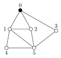
Figure 7: The original amnesiac flooding algorithm ${\cal A}_{\mathsf{AF}}$ terminates after 4 rounds for the graph of Fig. 1.

Appendix B Algorithm for Multi-Message Broadcast

In this section we describe the extension of algorithm ${\cal A}_{\mathsf{AFI}}$ to realize multi-message broadcasts. As with ${\cal A}_{\mathsf{AFI}}$ each node $v$ has two variables. First, a Boolean flag parity that is toggled at the end of every round. The values of parity must not be synchronized among nodes. The second variable corresponds to variable $M$ of ${\cal A}_{\mathsf{AF}}$, it is used to store the senders of the messages according to the parity of the round in which they were received. In multi-message broadcasts a node can receive different messages in a round and therefore must be prepared to separately store the senders of these messages. An associative array messTbl is used for this purpose. Message identifiers are the keys, the values correspond to variable $M$ of ${\cal A}_{\mathsf{AFI}}$. Values consist of two parts $list[\mathit{true}]$ and $list[\mathit{false}]$, corresponding to the round’s parity. The symbol $\bot$ indicates that no message has arrived in rounds with the specified parity. This is needed to distinguish this from the case when a node invokes a broadcast, in this case the value is the empty set $\emptyset$. If we insert a node $w$ when the value is $\bot$ then it is $\{w\}$ afterwards. Tab. 1 shows an example of messTbl.

Message Id	Message	$list[\mathit{true}]$	$list[\mathit{false}]$
$17$	$\ldots$	$v_{1},v_{3}$	$v_{1},v_{4}$
$123$	$\ldots$	$v_{15}$	$\bot$
$3$	$\ldots$	$\emptyset$	$\emptyset$

Table 1: Example of a node’s associative array messTbl.

Fig. 8 shows the pseudo code of the proposed extension of ${\cal A}_{\mathsf{AFI}}$. In every round the following three steps are executed: First, received messages are used to update the message table. In the second step a message is selected from the message table and sent to those neighbors not listed in the appropriate column of the corresponding row. As a last step the flag parity is toggled.

 

⬇

init:

parity$\;\coloneqq\;$true;

messTbl$\;\coloneqq\;$Create new HashMap with entries (id, m, list[])

In every round do:

1. foreach received message BC$\langle$id_m, m$\rangle$ from neighbor w do

if id $\!\!\not\in\!\!$ messTbl

Create new entry with (id_m, m, list[true]$\;\coloneqq\;$$\bot$, list[false]$\;\coloneqq\;$$\bot$)

in messTbl

if w $\!\!\not\in\!\!$ messTbl[id_m].list[parity]

if messTbl[id_m].list[parity]$\;=\;$$\bot$

messTbl[id_m].list[parity]$\;\coloneqq\;$$\big{\{}\big{\}}$

Add w to messTbl[id_m].list[parity]

foreach i $\!\!\in\!\!$ messTbl do

if messTbl[i].list[parity]$\;=\;$N(v)

messTbl[i].list[parity]$\;\coloneqq\;$$\bot$

if messTbl[i].list[parity]$\;=\;$$\bot$ and messTbl[i].list[$\overline{\texttt{parity}}$]$\;=\;$$\bot$

Delete entry i from messTbl

2. Select an entry i in messTbl with messTbl[i].list[parity]$\;\neq\;$$\bot$

foreach w $\!\!\in\!\!$ N(v) do

if w $\!\!\not\in\!\!$ messTbl[i].list[parity]

send(w,  BC$\langle$messTbl[i].id, messTbl[i].m$\rangle$)

messTbl[i].list[parity]$\;=\;$$\bot$

if (messTbl[i].list[$\overline{\texttt{parity}}$]$\;=\;$$\bot$ or messTbl[i].list[$\overline{\texttt{parity}}$]$\;=\;$$\emptyset$)

Delete entry i from messTbl

3. parity$\;\coloneqq\;$$\overline{\texttt{parity}}$

function broadcast(m)$\;:\;$

id$\;\coloneqq\;$Create unique message id for message m

Create new entry with (id, m, list[true]$\;\coloneqq\;$$\emptyset$, list[false]$\;\coloneqq\;$$\emptyset$)

in messTbl

 

Figure 8: Algorithm

Next we describe the first two steps at full length. The details of the first step are as follows. Any time a node $v$ receives a message $m$ with identifier $id$ from a neighbor $w$ it is checked whether $v$’s message table already contains a row for $id$. If not, a new row is created and the first two columns are filled with $id$ and $m$. The last two columns contain the symbol $\bot$. In any case the node $w$ is appended to the list in the third or forth column according to the current parity into $v.\textit{messTbl}[id].list$. In case the corresponding entry is $\bot$ a new list with the single element $w$ is created.

When all messages of a round are received then the following cleaning action is performed as the closing-off of the first step. All values in $v.\textit{messTbl}$ with the current parity are checked. If a value equals $N(v)$ then it is set to $\bot$. In this case $v$ received message $id$ from all neighbors and no action is required. After this cleaning step, an entry of messTbl is selected for which the value with the current parity is not $\bot$. Selection is performed according to a given criterion. The message belonging to this entry is sent to all neighbors but those listed in the entry. Finally the entry is set to $\bot$.

Initially for each node $v$ the associative array messTbl is empty and flag parity has an arbitrary value. A node $v$ that wants to disseminate a new message $m$ with the identifier $id$ creates a new row in the message table and inserts the value $id$ and $m$ into the first two columns. The last two columns contain the empty list $\emptyset$. The third row of Tab. 1 is an example for this situation.

If the node $v$ with the message table shown in Tab. 1 receives in a round with $\textit{parity}=\mathit{false}$ a message with $id=17$ from neighbors $v_{1},v_{5}$, and $v_{8}$ the last column of the corresponding row would be updated to $v_{1},v_{4},v_{5},v_{8}$. If the id of the received message is $123$ then the last column would be updated to $v_{1},v_{5},v_{8}$. Next we give an example for the execution of the second part of the algorithm for Tab. 1. If $\textit{parity}=\mathit{false}$ and the first row is selected, the message with $id=17$ is sent to all neighbors of $v$ except $v_{1}$ and $v_{4}$. If the last row is selected, the message with $id=3$ is sent to all neighbors. In the first case the last column is set to $\bot$ and the row remains in the table. In the second case the row is deleted. If on the other hand $\textit{parity}=\mathit{true}$ and the second row is selected the message with $id=123$ is sent to all neighbors of the node except node $v_{15}$ and the row is deleted from the table.

References

- [1] Alan Demers, Dan Greene, Carl Hauser, Wes Irish, John Larson, Scott Shenker, Howard Sturgis, Dan Swinehart, and Doug Terry. Epidemic algorithms for replicated database maintenance. In Proc. 6th Annual Symp. on Principles of Distributed Computing, PODC, page 1–12. ACM, 1987.
- [2] Walter Hussak and Amitabh Trehan. On the Termination of Flooding. In Christophe Paul and Markus Bläser, editors, 37th Symp. Theo. Aspects of Comp. Sc. (STACS), volume 154 of LIPIcs, pages 17:1–17:13, 2020.
- [3] David Peleg. Distributed Computing: A Locality-Sensitive Approach. SIAM Society for Industrial and Applied Mathematics, Philadelphia, 2000.
- [4] Volker Turau. Amnesiac Flooding: Synchronous Stateless Information Dissemination. In Proc. Int. Conf. on Current Trends in Theory and Practice of Computer Science (SOFSEM), volume ??? of LNCS, pages ???–???
- [5] Volker Turau. Stateless Information Dissemination Algorithms. In Proc. Int. Coll. on Structural Information and Communication Complexity (SIROCCO), volume 12156 of LNCS, pages 183–199, 2020.
- [6] Alan M. Frieze and Geoffrey R. Grimmett. The shortest-path problem for graphs with random arc-lengths. Discrete Applied Mathematics, 10(1):57 – 77, 1985.
- [7] Uriel Feige, David Peleg, Prabhakar Raghavan, and Eli Upfal. Randomized broadcast in networks. In Tetsuo Asano, Toshihide Ibaraki, and Hiroshi Imai, editors, Algorithms, pages 128–137. Springer, 1990.
- [8] Yves Mocquard, Bruno Sericola, and Emmanuelle Anceaume. Probabilistic analysis of rumor-spreading time. INFORMS Journal on Computing, 32(1):172–181, 2020.
- [9] Walter Hussak and Amitabh Trehan. Terminating cases of flooding. CoRR, abs/2009.05776, 2020.
- [10] M. Raynal, J. Stainer, J. Cao, and W. Wu. A simple broadcast algorithm for recurrent dynamic systems. In IEEE 28th Int. Conf. on Advanced Information Networking and Applications, pages 933–939, 2014.
- [11] Arnaud Casteigts, Paola Flocchini, Bernard Mans, and Nicola Santoro. Deterministic computations in time-varying graphs: Broadcasting under unstructured mobility. In Cristian S. Calude and Vladimiro Sassone, editors, Theoretical Computer Science, pages 111–124. Springer, 2010.