Spin diffusion and spin conductivity in the 2d Hubbard model

Abstract

We study the spin diffusion and spin conductivity in the square lattice Hubbard model by using the finite-temperature Lanczos method. We show that the spin diffusion behaves differently from the charge diffusion and has a nonmonotonic $T$ dependence. This is due to a progressive liberation of charges that contribute to spin transport and enhance it beyond that active at low temperature due to the Heisenberg exchange. We further show that going away from half-filling and zero magnetization increases the spin diffusion, but that the increase is insufficient to reconcile the difference between the model calculations and the recent measurements on cold-atoms.

I Introduction

Non-saturating metallic resistivity $\rho$ that exceeds the Mott-Ioffe-Regel (MIR) value (estimated with the scattering length $l$ equal to the lattice spacing, $l\sim a$) is a characteristic property of strongly correlated metals. Recent theoretical work Kokalj (2017); Perepelitsky et al. (2016) found that within the Hubbard model, such behavior of conductivity $\sigma_{c}=1/\rho$ can be understood via Nerst-Einstein relation, $\sigma_{c}=D_{c}\chi_{c}$, with a saturating diffusion constant $D_{c}$ and strongly suppressed charge susceptibility at elevated temperatures. Cold-atom experiments Brown et al. (2019) have verified this behavior, which established that at least the high-temperature regime of the charge transport is fully understood.

Simultaneously, cold-atoms were also used to probe much less explored quantities: the spin conductivity $\sigma_{s}$ and spin diffusion constant $D_{s}$ Nichols et al. (2019) (the spin current that flows as a response to the magnetic field or magnetization gradient). These quantities are not only important from the theoretical point of view (as the interplay between spins and charges lies at the heart of the strong-correlation problem Anderson (1997); Lee et al. (2006)) but are important also, e.g., for the applications in spintronics Žutić et al. (2004); Chumak et al. (2015); Hirohata et al. (2020), for heat transferZotos et al. (1997); Sologubenko et al. (2001); Hess et al. (2001), and further to understand the behavior of the NMR relaxation rate Sokol et al. (1993); Larionov (2004); Yusuf et al. (2007). $\sigma_{s}$ or $D_{s}$ can be indirectly estimated via heat conductivity or NMR relaxation rate, but also more directly through the spin injection technique Johnson (1993); Si (1997); Ji et al. (2004) and magnetization currents measurements Meier and Loss (2003); Cornelissen et al. (2015).

Importantly, in correlated materials, the spins and charges do not behave alike and they exhibit a so-called spin-charge separation Anderson (1997); Lee et al. (2006), which means one cannot infer the behavior of spin degrees of freedom (e.g., $\sigma_{s}$, $D_{s}$ and $\chi_{s}$), based on the measurements of charge properties (e.g., $\sigma_{c}$, $D_{c}$ and $\chi_{c}$), and vice versa. The question that arises is, how strong is the spin-charge separation in different temperature ($T$) regimes? Can one understand also the spin transport more simply in terms of the Nernst-Einstein relation? Does $D_{s}$ saturate and to what value? The cold-atom experiment Nichols et al. (2019) has not analyzed this behavior in detail, and, intriguingly reported an inconsistency with the numerical linked-cluster expansion (NLCE) method.

In this paper we consider these questions by solving the Hubbard model with the finite-temperature Lanczos method (FTLM). We find that spin transport at high $T$ can be understood in terms of the Nernst-Einstein relation, but the behavior is richer than the one for the charge transport. $D_{s}$ has a nonmonotonic $T$ dependence and experiences an increase at high $T$ on the crossover between two saturated regimes: the lower-$T$ one at $T$ of the order of Heisenberg exchange $J$ with strong spin-charge separation and the asymptotic high-$T$ one, where the spins and charges behave alike. The scattering length remains of the order of lattice spacing throughout this crossover and the behavior is explained in terms of the evolution of effective velocity, instead.

Previously, the spin diffusion in 2d lattices was considered for the Heisenberg model, namely with high-$T$ frequency moments Bennett and Martin (1965); Sokol et al. (1993), with theory of Blume and Hubbard Nagao and Igarashi (1998), with interacting spin wave theory Sentef et al. (2007); Pires and Lima (2009) and with numerical Bonča and Jaklič (1995) and Mori-Zwanzig Larionov (2004) approach to the $t$-$J$ model. The spin diffusion in the Hubbard model was considered with Gaussian extrapolation of short-time dynamics in the weak-coupling limit Kopietz (1998), and with NLCE Nichols et al. (2019). To our knowledge, the $T$ dependence of $D_{s}$ in the Hubbard model, has not been numerically calculated so far.

This paper is structured as following: we briefly present the method in section II then present the results for dynamical conductivity in section III and for spin diffusion in section IV. We comment on a phenomenological explanation for these results in section V and comment on the effect of doping and magnetization in section VI. Appendix A contains a derivation of the sum rule for dynamical spin conductivity while Appendix B, C and E contain further details on the calculated quantities.

II Model and method

We consider the Hubbard model on the square lattice,

$$H=-t\sum_{\langle i,j\rangle,s}c^{\dagger}_{i,s}c_{j,s}+U\sum_{i}n_{i,\uparrow}n_{i,\downarrow},$$ (1)

where $c^{\dagger}_{i,s}/c_{i,s}$ create/annihilate an electron of spin $s$ (either $\uparrow$ or $\downarrow$) at the lattice site $i$. $t$ is the hopping amplitude between the nearest neighbors and we use it as the energy units. We further set $\hbar=k_{B}=e=g\mu_{B}=1$. We denote the lattice constant with $a$.

We solve the model with FTLM Jaklič and Prelovšek (2000); Prelovšek and Bonča (2013); Kokalj and McKenzie (2013), which uses the Lanczos algorithm to obtain approximate eigenstates of the Hamiltonian and additional sampling over the initial random vectors to treat finite-$T$ properties on small clusters. We use $N=4\times 4$ cluster. To reduce the finite-size effects that appear at $T\lesssim t$ we further employ averaging over twisted boundary conditions and use the grand canonical ensemble. This allows us to reach reliable results, e.g, for $U=10t$, at $T\gtrsim 0.2t$ for the thermodynamic quantities (e.g., spin susceptibility $\chi_{s}$), and at $T\gtrsim 0.8t$ for dynamical quantities (e.g., dc spin conductivity $\sigma_{s}$). We omit low-$T$ results for which, due to finite size, dynamical spin stiffness exceeds 1% of the total spectral weight.

To calculate $D_{s}$ (and analogously the charge diffusion constant $D_{c}$) we use the Nernst-Einstein relation (see, e.g., Refs. Kopietz, 1998; Pakhira and McKenzie, 2015 for derivation)

$$\sigma_{s}=D_{s}\chi_{s}.$$ (2)

The dc spin conductivity $\sigma_{s}$ is calculated as the $\omega=0$ value of the dynamical spin conductivity $\sigma_{s}(\omega)$, which is directly evaluated as the current-current correlation functionJaklič and Prelovšek (2000); Kokalj (2017). $\sigma_{s}(\omega)$ for finite cluster consists of delta functions which need to be broadened. This introduces some uncertainty in dynamical results and we estimate the uncertainty due to finite-size effects and broadening to be $\lesssim 10\%$.

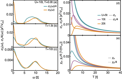
Figure 1: Dynamical spin conductivity $\sigma_{s}(\omega)$ and charge conductivity $\sigma_{c}(\omega)$. At low $T$ (a) $\sigma_{s}(\omega)$ shows a large Drude-like peak and the conducting character, while $\sigma_{c}(\omega)$ shows an insulating behavior with only a small value at $\omega\sim 0$. At intermediate temperature $J<T<U$ (b) low-$\omega$ peak in $\sigma_{s}(\omega)$ develops a shoulder like structure. At high $T$ (c) $\sigma_{s}(\omega)$ and $\sigma_{c}(\omega)$ become similar. Comparison (d) of $\sigma_{s}$ and $\sigma_{c}$, which are similar for $T\gtrsim U/2$, and comparison (e) of $\chi_{s}$ and $\chi_{c}$. Results are for half-filling ($p=1-n=0$).

III Dynamical conductivity

In Fig. 1(a-c) we show the dynamical spin $\sigma_{s}(\omega)$ and charge $\sigma_{c}(\omega)$ conductivities for the half-filled Hubbard model at half-filling for $U=10t$. The two quantities behave very similarly at high $T$, and both display a low-$\omega$ “Drude” peak, and a high-$\omega$ peak at $\omega\sim U$ due to transitions to Hubbard bands.

On cooling down, there is a growing degree of the spin-charge separation. The charge transport is depleted and the low-$\omega$ peak in $\sigma_{c}(\omega)$ is suppressed, corresponding to the Mott insulating regime. Conversely, in the spin conductivity, a peak develops at $\omega\sim 0$, corresponding to a spin-metallic regime in the spin sector (see also Fig. 1(d) for the $T-$dependence of the dc transport). The two quantities $\sigma_{s}(\omega)$ and $\sigma_{s}(\omega)$ are actually never fully independent as they are related by the f-sum rule. Namely, their integrals over frequency are equal up to a factor of 4 Fishman and Jarrell (2002) as we show in Appendix A. This also means that at low $T$, parts of the spectral weight in $\sigma_{s}(\omega)$ is in comparison to $\sigma_{c}(\omega)$ removed from the Hubbard band to accommodate the increase at low $\omega$. One can relate the behavior of $\sigma_{c,s}(\omega)$ to charge and spin fluctuations, e.g., $\sigma_{c,s}(\omega)=\lim_{q\to 0}\frac{\omega}{q^{2}}\textrm{Im}[\chi_{c,s}(q,\omega)]$. Here, $\chi_{c,s}(q,\omega)$ are the dynamical susceptibilities. Relative to the charge sector, on lowering $\omega$ the spin fluctuations are first suppressed and then increased. One can also notice, that $\sigma_{s}(\omega)$ at intermediate $T$ develops an interesting two peak like structure at $\omega\sim 0$ (see Fig. 1(b)), i.e., a sharper peak on top of the broader peak both centered at $\omega=0$. Notice also that whereas the key distinction between the behavior of spins and charges could be expected at the energy scales of the order Heisenberg exchange $J=4t^{2}/U$, the two conductivities differ also at larger energy scales.

It is worth mentioning, that the difference between $\sigma_{s}(\omega)$ and $\sigma_{c}(\omega)$ vanishes at the bubble level and appears due to the vertex correction (see, e.g., Refs. Fishman and Jarrell, 2002; Vučičević et al., 2019; Vranić et al., 2020). Their difference is therefore a direct indication of the importance of vertex corrections.

In Fig. 1(e) we show also the $T$ dependence of spin and charge susceptibilities $\chi_{s,c}$. One sees a clear distinction between $\chi_{c}$, that decreases at low-$T$ indicating a charge gap and large values of $\chi_{s}$ indicating large local-moment and Curie-Weiss-like behavior. See Appendix C for more details.

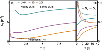
Figure 2: (a) Spin diffusion constant $D_{s}$ for half-filled Hubbard model for $U/t=5,10,20$. $D_{s}$ decreases with increasing $U$ and shows a nonmonotonic $T$ dependence. As $T\to 0$ one expects diverging $D_{s}$ due to increased spin coherenceBonča and Jaklič (1995); Nagao and Igarashi (1998); Kopietz (1998), which shows up as a small upturn in our results. The divergence is indicated by showing the result of a Blume and Hubbard theory for the Heisenberg model from Nagao et al. Nagao and Igarashi (1998) for $U=20t$. In the intermediate regime $J\ll T\ll U$, $D_{s}$ is minimal and for large $U$ shows a saturating behavior corresponding to the high-$T$ Heisenberg result Sokol et al. (1993) and agrees with FTLM result for the Heisenberg model (Bonča et al. Bonča and Jaklič (1995)). (b) As $T$ increases further, $D_{s}$ shows an increase and saturates for $T\to\infty$ at the same value as the charge diffusion $D_{c}$ and in accordance with the standard Mott-Ioffe-Regel limit.

IV Spin diffusion

We now turn to the $T$ dependence of the diffusion constant. Fig. 2(a) shows $D_{s}$ vs. $T$ for several $U$. Even though the spin conductivities are all metallic, $D_{s}$ shows an unusual nonmonotonic $T$ dependence. Unlike in the case of charge transport in metals (where $D_{c}$ monotonously increases with lowering $T$), $D_{s}$ initially drops, reaches a minimum and only at lowest available $T$ starts to grow. The growth of $D_{s}$ in this low-$T$ regime can be discussed in terms of a growing correlation length and associated coherence of spin-waves in the Heisenberg modelNagao and Igarashi (1998); Chakravarty et al. (1989) and associated longer mean free path $l_{s}$ (as $D_{s}\sim v_{s}l_{s}/2$ with $v_{s}$ a characteristic spin velocity). To indicate the expected behavior, we supplement our results in Fig. 2(a)) with a result of Nagao et al.Nagao and Igarashi (1998) for the Heisenberg model.

At intermediate $T$ ($\sim 2t$), $D_{s}$ reaches a minimum with indications for intermediate saturating behavior seen for larger $U$. In the regime of $T\ll U$ for large $U$, the behavior becomes that of the Heisenberg model and is therefore entirely controlled by $J$. The calculated $D_{s}$ hence agrees with the results from Heisenberg model, including high-$T$ moments expansion Sokol et al. (1993), numerical FTLM Bonča and Jaklič (1995) and with self-consistent Blume and Hubbard theory Nagao and Igarashi (1998). $D_{s}$ further shows in a regime $J\ll T\ll U$ a saturation towards the high-$T$ limit of the Heisenberg model Sokol et al. (1993); Bonča and Jaklič (1995) with $D_{s}\sim 0.40Ja^{2}$, see results for $U=20t$ in Fig. 2(a). Such high-$T$ value can be understood in terms of a “spin Mott-Ioffe-Regel” value by approximating the spin-wave velocity to $v_{s}\sim\frac{4Ja}{\sqrt{2}\pi}$ and $l_{s}$ to minimal or MIR limiting value $l_{s}\sim a$. This leads to $D_{s}\sim v_{s}l_{s}/2\sim 0.45Ja^{2}$.

With further increase of $T$ towards $U$, $D_{s}$ remarkably increases. This is in contradiction with a naive expectation of decreasing mean free path (increasing scattering rate) and therefore decreasing $D_{s}$ with increasing $T$. The reason for this can be found in the increase of empty and doubly occupied sites allowing for new conducting and diffusive mechanism of spin in terms of electron hopping, in addition to exchange mechanism dominating at low $T$.

Fig. 2(b) additionally shows the charge diffusion constants compared to $D_{s}$ in a broader $T$ range. One notices that $D_{c}$ decreases on heating up (which is the standard behavior) and that $D_{c}$ and $D_{s}$ approach each other at very high $T$. There, both $D_{s}$ and $D_{c}$ saturate at the usual MIR limit $D\sim at^{2}$.

It is interesting to observe that in a broad temperature regime $T\gtrsim U/2$ the conductivities $\sigma_{s}$ and $\sigma_{c}$ differ little ($<20$%) (Fig. 1(d)), while the corresponding diffusion constants differ by a factor of almost 2, (Fig. 2(b)). The difference between $D_{s}$ and $D_{c}$ is compensated by the inverse difference between susceptibilities $\chi_{s}$ and $\chi_{c}$ (Fig. 1(e)) to give similar conductivities in the whole $T\gtrsim U/2$ regime. This suggest an intriguing relationship between the diffusion (dynamic) and susceptibility (static property).

In passing we mention also that in the high-$T$ limit ($T\gg U$), $D_{s}$ does not show the $t^{2}/U$ scaling, as suggested from the moment expansion analysis Kopietz (1998). This can be traced back to the two peak structure in the dynamical spin conductivity (Fig. 1) with the upper Hubbard peak positioned at $\omega\sim U$, which is quite challenging to correctly reproduce from the frequency moments.

V Mean free path

It is instructive to investigate the phenomenology of our results in more details. From the width of the low frequency peak in $\sigma_{s}(\omega\sim 0)$ (e.g., Fig. 1(a-c)) we estimate a spin scattering time $\tau_{s}$ (see also Appendix E). Then we use a simple relation $D_{s}\sim\frac{v_{s}^{2}\tau_{s}}{2}$ and the values of $D_{s}$ to estimate the spin velocity $v_{s}$ and further the spin mean free path $l_{s}\sim v_{s}\tau_{s}$. The results are plotted on Fig. 3, and reveal evolution between two regimes, a lower-$T$ one governed by the scale $J$ and a higher-$T$ one governed by $t$. $\tau_{s}$ is seen to exhibit a pronounced increase below $T\sim U/2$, which coincides with a sharp structure of width $1/\tau_{s}\sim J$ emerging in the dynamical spectra. At $T\gtrsim U/2$ it saturates at the value of order $1/\tau_{s}\sim t$. The extracted characteristic velocity starts at values $v_{s}\sim Ja$ at low $T$ and increases monotonically to the value of $v_{s}\sim ta$. The low-$T$ estimate of $v_{s}\sim 0.6ta$ for $U=10t$ (Fig. 3(b)) is remarkably close to the estimate of $v_{s}\sim 1.6Ja\sim 0.64ta$ within the Heisenberg modelKim and Troyer (1998), in particular, since we used a rough approximation $D_{s}\sim v_{s}^{2}\tau_{s}/2$.

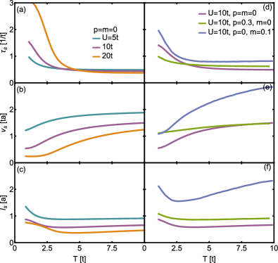
Figure 3: $T$ dependence of spin scattering time $\tau_{s}$, spin velocity $v_{s}$ and spin mean free path $l_{s}$ for several choices of interaction strength $U$, hole doping $p$ and magnetization $m$.

Conversely, $l_{s}$ is to a good approximation $T$ independent and close to the lattice spacing. It shows only a moderate increase at lowest $T$. The spin transport is thus characterized by a saturated scattering length throughout the considered $T$ regime (except at lowest $T$) and the effects seen in the diffusion constant are explained in terms of progressive unbinding of the charge degrees of freedom that progressively increase the corresponding velocity to a value given by $t$ instead of $J$. In the half-filled case, this increase of $v_{s}$ is the main reason for the increase of $D_{s}\sim v_{s}l_{s}/2$ with increasing $T$ (see Fig. 2). We note that the dependence of $l_{s}$ on $U$ in Fig. 2(c) is smaller at higher $T$($>U$) and $l_{s}$ is closer to $a$ for all $U$.

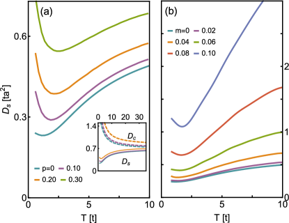
Figure 4: (a) Increase of spin diffusion $D_{s}$ with doping $p$. (Inset) In the whole shown $T$ and $p$ regime $D_{s}$ is smaller and behaves qualitatively differently than $D_{c}$, even at largest $p=0.3$. They become similar only in the very high $T$ limit. $U=10t$. (b) $D_{s}$ vs. $T$ for several values of magnetizations $m$. With increasing $m$, $D_{s}$ increases in whole $T$ range. $U=10t$, $p=0$.

VI Doping and magnetization effect

How is this picture modified at finite dopings and magnetizations? Because moving electrons carry both spin and charge, one could expect that away from half-filling, when the system is metallic, $D_{s}$ and $D_{c}$ behave more similarly. In Fig. 4(a) we show the behavior of $D_{s}$ for several dopings $p=1-n$. $n$ is the electron density. One clearly observes the increase of $D_{s}$ with increasing $p$, which is understood as opening of a new conducting channel via hopping of itinerant electrons or holes. The increase is particularly strong at lowest calculated $T$ and the indication of diverging $D_{s}(T\to 0)$ becomes more apparent. In doped case, $D_{s}$ approaches $D_{c}$, but $D_{s}$ and $D_{c}$ still behave distinctly (Fig. 4 (inset)), with $D_{s}$ having much smaller values and a pronounced minimum at intermediate $T$. Thus, doping diminishes the degree of spin-charge separation, but does not wash it out completely. At low-$T$, $D_{s}$ is much smaller than $D_{c}$ and the spin transport is less coherent than the charge transport, possibly due to stronger coupling to low lying spin excitations. The extracted $l_{s}$ remains roughly $T$ independent (Fig. 3(f)) and is somewhat larger, but still $l_{s}\sim a$. The extracted $v_{s}$ and $\tau_{s}$ show less $T$ dependence than in the undoped case (Fig. 3(d-e)).

The dependence on magnetization $m=\langle S_{z,tot}\rangle/N$ is shown on Fig. 4(b). It is found to be initially weak but becomes strong with increasing $m$. The results for $m=0.1$ deviate significantly from nonmagnetized ones, e.g., $D_{s}$ is increased by more than a factor of 4. The underlying physics differs from the case of charge doping: with increasing $m$ one stays in, or even goes deeper into, the Mott insulating phase (see Fig. 1 and 2 in Ref. Prelovšek et al., 2015). The increase of $D_{s}$ is therefore not due to mobile electron-like particles, but rather due to weaker scattering of spin waves and their longer $l_{s}$. This is indeed revealed in Fig. 3(f), where $l_{s}$ is increased due to increase of both $v_{s}$ and $\tau_{s}$. With increasing $m$ the Hubbard interaction becomes less effective and one approaches the limit of noninteracting spins or single noninteracting holon-doublon pairPrelovšek et al. (2015) (the limit of only one $\downarrow$ spin in the background of $\uparrow$ spins). The strong increase of $D_{s}$ with increasing $T$ at $T\gtrsim 2t$ is mainly due to increasing $v_{s}$, but surprisingly, also $l_{s}$ moderately increases with increasing $T$ as well.

VII Discussion

We compared our results to the $D_{s}$ and $\sigma_{s}$ measured in the cold atom experimentNichols et al. (2019), see Fig. 5, where the measured $D_{s}$ and $\sigma_{s}$ are found to be by about a factor of 2 higher than the NLCE results for the Hubbard model. Our results agree well with the NLCE results. As discussed in Sec. VI., $D_{s}$ and $\sigma_{s}$ are increased by magnetization. We estimate that the experimental deviation from half-filling and zero magnetization are too small to understand the discrepancy between the numerics and experiment in those terms.

We also compare our results (see Appendix D) with the diffusion bound $D_{s}>v_{s}^{2}/T$ suggested from holographic dualityHartnoll (2015). Using our rough estimate for $v_{s}$ extracted from $D_{s}$ and $\tau_{s}$, we observe that the bound is obeyed in most of the explored parameter regime except at small $U$, where it is mildly violated. We also observe that $D_{s}$ does not follow or has a $T$ dependence close to the proposed bound in the calculated $T$ regime. See also Ref. Pakhira and McKenzie, 2015.

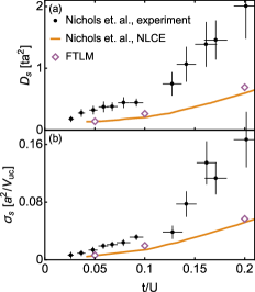
Figure 5: Comparison of our FTLM results with experimental dataNichols et al. (2019) and numerical NLCE resultsNichols et al. (2019). FTLM results are for fixed entropy density of $1.1k_{B}$, which was estimated for experiment and taken also in the NLCE calculations.

VIII Conclusions

We have shown that $D_{s}$ has a striking nonmonotonic $T$-dependence, which can be understood in terms of a crossover from a low-$T$ spin-wave dominated regime to a high-$T$ asymptotic regime via an intermediate strong spin-charge separation regime, where it nearly saturates according to the high-$T$ Heisenberg model result at $D_{s}\sim Ja^{2}$. In both of these high-$T$ regimes, the scattering length is of the order lattice spacing and the conductivity is strongly reduced due to decreased $\chi_{s}$. In analogy to the case of charge transport, these regime can be referred to as a “spin bad metal”. The action in $D_{s}$ is governed by the spin velocity that evolves from $J$ to $t$ up to the asymptotic high-$T$ regime, where spins and charges behave alike and $D_{s}\sim D_{c}\sim ta^{2}$.

In the whole regime of $T\lesssim U/2$ (with or without doping or magnetization) the spins and charges behave differently. An interesting open question is better characterization of the behavior at lower $T$. Away from half-filling in the well-defined quasiparticle regime one expects similar behavior of spin and charge transport. Further studies in real materials, e.g., with techniques like spin injection Johnson (1993); Si (1997); Ji et al. (2004) or magnetization currents measurements Meier and Loss (2003); Cornelissen et al. (2015) would be highly valuable. Better understanding of the spin transport would also shed light on thermal conductivity and NMR relaxation rateTakigawa et al. (1996), for which our results suggest a nonmonotonic-in-$T$ diffusive contribution.

Appendix A Sum rule

To derive the spectral sum rule for the dynamical spin conductivity we employ the approach by B. S. ShastryShastry (2008). The sum rule is given by the expectation value of the stress tensor $\mathcal{T}$

$$\int_{-\infty}^{\infty}\sigma_{c,s}(\omega)d\omega=\frac{\pi\langle\mathcal{T}_{c,s}\rangle}{N}.$$ (3)

Supscripts $c$ and $s$ stand for charge and spin quantities, respectively. The charge stress tensor is given byShastry (2008)

$$\mathcal{T}_{c}=-\lim_{q\to 0}\frac{d}{dq}[j_{c}(q),n(-q)],$$ (4)

where the charge current and charge density operators are

$$j_{c}(q) = it\sum_{i,\delta,s}\delta_{x}c^{\dagger}_{i+\delta,s}c_{i,s}\textrm{e}^{iq(R_{i,x}+\delta_{x}/2)},$$ (5)

$$n(q) = \sum_{i,s}n_{i,s}\textrm{e}^{iqR_{i,x}}.$$ (6)

Here, the $x$ direction of current and of the wave vector $q$ is explicitly used. $\delta$ goes over all nearest neighbors and $\delta_{x}$ denotes the spacial distance to neighboring site in $x$ direction. $R_{i,x}$ is the $x$ coordinate of site $i$. Similarly one can write the spin stress tensor

$$\mathcal{T}_{s}=-\lim_{q\to 0}\frac{d}{dq}[j_{s}(q),m(-q)],$$ (7)

and the spin current and magnetization density operators,

$$j_{s}(q) = it\sum_{i,\delta,s}s\delta_{x}c^{\dagger}_{i+\delta,s}c_{i,s}\textrm{e}^{iq(R_{i,x}+\delta_{x}/2)},$$ (8)

$$m(q) = \sum_{i,s}sn_{i,s}\textrm{e}^{iqR_{i,x}}.$$ (9)

Here the factor $s$ in the sums for $j_{s}(q)$ and $m(q)$ is taken to be $1/2$ for $\uparrow$ spins and $-1/2$ for $\downarrow$ spins. Evaluating the commutation in expressions for $\mathcal{T}_{c}$ in Eq. 4 and for $\mathcal{T}_{s}$ in Eq. 7 together with $q$-derivative and limit, one obtains similar expressions for $\mathcal{T}_{c}$ and $\mathcal{T}_{s}$.

$$\mathcal{T}_{c} = t\sum_{i,\delta,s}\delta_{x}^{2}c_{i+\delta,s}^{\dagger}c_{i,s},$$ (10)

$$\mathcal{T}_{s} = t\sum_{i,\delta,s}s^{2}\delta_{x}^{2}c_{i+\delta,s}^{\dagger}c_{i,s}.$$ (11)

The reason for the only difference of factor $s^{2}=1/4$ in expression for $\mathcal{T}_{s}$ (11), in comparison to $\mathcal{T}_{c}$ (10), is the commutation of spin $\uparrow$ and $\downarrow$ operators and no spin mixed terms in the sums for currents and density operators (Eqs. 5, 6, 8 and 9). The expectation values of $\mathcal{T}_{c}$ and $\mathcal{T}_{s}$ correspond to the expectations values of the kinetic energy for our nearest-neighbor Hubbard model Jaklič and Prelovšek (2000)

$$\langle\mathcal{T}_{c}\rangle = \frac{a^{2}}{2}\langle H_{kin}\rangle,$$ (12)

$$\langle\mathcal{T}_{s}\rangle = \frac{a^{2}}{8}\langle H_{kin}\rangle.$$ (13)

This leads to the (optical) sum rule given in the main text.

$$\int_{-\infty}^{\infty}\sigma_{c}(\omega)d\omega = \frac{\pi a^{2}}{2N}\langle H_{kin}\rangle,$$ (14)

$$\int_{-\infty}^{\infty}\sigma_{s}(\omega)d\omega = \frac{\pi a^{2}}{8N}\langle H_{kin}\rangle,$$ (15)

with the difference only of a factor of 1/4.

Appendix B Finite size effects

To estimate the error due to finite size effects, we plot the optical spin conductivity for different system sizes on Fig. 6. We find that they differ substantially only around $\omega=0$. This is the basis for the error estimate given in the main text.

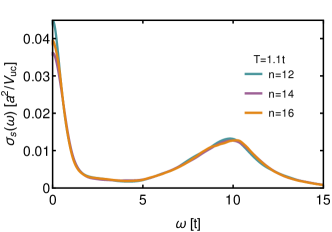
Figure 6: Comparison of the optical spectrum of spin conductivity obtained on different size clusters. We use 16 different periodic boundary conditions for $N=12$ and $N=14$ and 8 for $N=16$.

Appendix C Resistivity

It is instructive to inspect also the inverse conductivity, namely the resistivity $\rho=1/\sigma$. See Fig. 7(a). Linear in $T$ resistivity is easily recognized for both $\rho_{c}$ and $\rho_{s}$ at high $T$ and $\rho_{c}$ shows a pronounced crossover into the insulating regime at low $T$, while $\rho_{s}$ remains metallic. Spin susceptibility $\chi_{s}$ shows (Fig. 7(b)) an increase below $T\sim U$ and approaches the value of the high-$T$ Heisenberg limit with $T\chi_{s}=1/4$, which is expected for large $U$ and $J\ll T\ll U$. In the ultra high $T$ limit, $T\gg U$, both $T\chi_{s}$ and $T\chi_{c}/4$ approach the atomic limit of $1/8$.

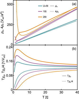
Figure 7: (a): Spin and charge resistivities. The later is multiplied by 4 to aid the comparison. (b) Spin and charge susceptibilities multiplied by temperature.

Appendix D Diffusion bound

We compare FTLM results to the conjectured lower bound on diffusion Hartnoll (2015), given by

$$D_{s}\gtrsim D_{H}=\frac{v_{s}^{2}}{T},$$ (16)

for some characteristic velocity $v_{s}$. While we cannot directly evaluate the velocity, we can estimate it using the non-interacting-like models. We take $v_{s}=\frac{4Ja}{\sqrt{2}\pi}$ as a typical velocity of spins deep in the Mott-insulating phase and $v_{s}=\frac{8ta}{\sqrt{2}\pi}$ as a typical speed of electrons. The real velocity is expected to be close to and interpolate between these two values. Our best estimate of velocity $v_{s}$ is obtained via calculation of $D_{s}$ and $\tau_{s}$ (see Fig. 9) and using the approximate relation $D_{s}=v_{s}^{2}\tau_{s}/2$ as discussed in the main text. We use these three velocites to estimate the various diffusion bounds and compare them with our FTLM results in Fig. 8.

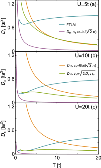
Figure 8: Comparison of $D_{s}$ calculated with FTLM results for various $U$ to the conjectured diffusion boundHartnoll (2015) $D_{H}=v_{s}^{2}/T$. If the bound is valid, the calculated $D_{s}$ (denoted with FTLM) would be larger than $D_{H}$. Due to uncertainty of $v_{s}$, which is needed to evaluate $D_{H}$, we compare to three values of $D_{H}$ obtained with three estimates for $v_{s}$. Our best estimate of $v_{s}$ is obtained via $\tau_{s}$ and the corresponding $D_{H}$ is shown with green line. At lowest $T$, our results indicate possible violation of the proposed bound.

We observe no apparent violation of the bound for $v_{s}=\frac{4Ja}{\sqrt{2}\pi}$, strong violation of the bound for $v_{s}=\frac{8ta}{\sqrt{2}\pi}$, while for our best estimate of $v_{s}=\sqrt{2D_{s}/\tau_{s}}$ there is an indication of diffusion bound violation at lowest-$T$. It is most apparent for $U=5t$, as shown in Fig. 8(a). However, due to rough estimate of $v_{s}$, we do not consider this as a clear-cut violation. We do, however, remark that the proposed bound does not manifest in any clear way in our results (in distinction with the Mott-Ioffe-Regel value).

Figure 9: Lorentz curve fitted to the low-$\omega$ structure in $\sigma_{s}(\omega)$ for $U=10$ and several $T$. For fitting we consider only $\omega\leq 2t$. We estimate the uncertainty of the extracted scattering time to be $\sim 30\%$ at low $T$ and $\sim 5\%$ at $T\gtrsim U/2$.

Appendix E Scattering time

To estimate the spin scattering time, we fit the Lorentz curve to the low-$\omega$ part of $\sigma_{s}(\omega)$. For illustration see Fig. 9. We choose to fit in the frequency range from $\omega=0$ to $\omega=2t$. Due to the dependence of extracted width ($1/\tau_{s}$) on frequency range and other possible prescriptions, e.g., taking the half width at half maximum, our value of $\tau_{s}$ should be taken as a rough estimate. We estimate its uncertainty to about 30%, and to be largest at lowest $T$. This uncertainty is then translated also to the uncertainty in the spin velocity $v_{s}$ and mean-free-path $l_{s}$. We note that the spectra at low-$\omega$ are a bit sharper and more linear than the Lorentz curve. Quite linear in $\omega$ behavior was, e.g., observed in the optical conductivity for the $t$-$J$ model Jaklič and Prelovšek (2000), where comparable $\omega$ resolution can be reached with smaller number of Lanczos steps. For a recent discussion, see Ref. Schönle et al., 2020.

References

- Kokalj (2017) J. Kokalj, Phys. Rev. B 95, 041110 (2017).
- Perepelitsky et al. (2016) E. Perepelitsky, A. Galatas, J. Mravlje, R. Žitko, E. Khatami, B. S. Shastry, and A. Georges, Phys. Rev. B 94, 235115 (2016).
- Brown et al. (2019) P. T. Brown, D. Mitra, E. Guardado-Sanchez, R. Nourafkan, A. Reymbaut, C.-D. Hébert, S. Bergeron, A.-M. S. Tremblay, J. Kokalj, D. A. Huse, P. Schauß, and W. S. Bakr, Science 363, 379 (2019).
- Nichols et al. (2019) M. A. Nichols, L. W. Cheuk, M. Okan, T. R. Hartke, E. Mendez, T. Senthil, E. Khatami, H. Zhang, and M. W. Zwierlein, Science 363, 383 (2019).
- Anderson (1997) P. W. Anderson, Phys. Today 10, 42 (1997).
- Lee et al. (2006) P. A. Lee, N. Nagaosa, and X.-G. Wen, Rev. Mod. Phys. 78, 17 (2006).
- Žutić et al. (2004) I. Žutić, J. Fabian, and S. Das Sarma, Rev. Mod. Phys. 76, 323 (2004).
- Chumak et al. (2015) A. V. Chumak, V. I. Vasyuchka, A. A. Serga, and B. Hillebrands, Nat. Phys. 11, 453 (2015).
- Hirohata et al. (2020) A. Hirohata, K. Yamada, Y. Nakatani, I.-L. Prejbeanu, B. Diény, P. Pirro, and B. Hillebrands, J. Magn. Magn. Mater. 509, 166711 (2020).
- Zotos et al. (1997) X. Zotos, F. Naef, and P. Prelovšek, Phys. Rev. B 55, 11029 (1997).
- Sologubenko et al. (2001) A. V. Sologubenko, K. Giannò, H. R. Ott, A. Vietkine, and A. Revcolevschi, Phys. Rev. B 64, 054412 (2001).
- Hess et al. (2001) C. Hess, C. Baumann, U. Ammerahl, B. Büchner, F. Heidrich-Meisner, W. Brenig, and A. Revcolevschi, Phys. Rev. B 64, 184305 (2001).
- Sokol et al. (1993) A. Sokol, E. Gagliano, and S. Bacci, Phys. Rev. B 47, 14646 (1993).
- Larionov (2004) I. A. Larionov, Phys. Rev. B 69, 214525 (2004).
- Yusuf et al. (2007) E. Yusuf, B. J. Powell, and R. H. McKenzie, Phys. Rev. B 75, 214515 (2007).
- Johnson (1993) M. Johnson, Phys. Rev. Lett. 70, 2142 (1993).
- Si (1997) Q. Si, Phys. Rev. Lett. 78, 1767 (1997).
- Ji et al. (2004) Y. Ji, A. Hoffmann, J. S. Jiang, and S. D. Bader, App. Phys. Lett. 85, 6218 (2004).
- Meier and Loss (2003) F. Meier and D. Loss, Phys. Rev. Lett. 90, 167204 (2003).
- Cornelissen et al. (2015) L. J. Cornelissen, J. Liu, R. A. Duine, J. B. Youssef, and B. J. van Wees, Nat. Phys. 11, 1022 (2015).
- Bennett and Martin (1965) H. S. Bennett and P. C. Martin, Phys. Rev. 138, A608 (1965).
- Nagao and Igarashi (1998) T. Nagao and J.-i. Igarashi, J. Phys. Soc. Japan 67, 1029 (1998).
- Sentef et al. (2007) M. Sentef, M. Kollar, and A. P. Kampf, Phys. Rev. B 75, 214403 (2007).
- Pires and Lima (2009) A. S. T. Pires and L. S. Lima, Phys. Rev. B 79, 064401 (2009).
- Bonča and Jaklič (1995) J. Bonča and J. Jaklič, Phys. Rev. B 51, 16083 (1995).
- Kopietz (1998) P. Kopietz, Phys. Rev. B 57, 7829 (1998).
- Jaklič and Prelovšek (2000) J. Jaklič and P. Prelovšek, Adv. Phys. 49, 1 (2000).
- Prelovšek and Bonča (2013) P. Prelovšek and J. Bonča, Strongly Correlated Systems: Numerical Methods, edited by A. Avella and F. Mancini, Springer Series in Solid-State Sciences (Springer Berlin Heidelberg, 2013).
- Kokalj and McKenzie (2013) J. Kokalj and R. H. McKenzie, Phys. Rev. Lett. 110, 206402 (2013).
- Pakhira and McKenzie (2015) N. Pakhira and R. H. McKenzie, Phys. Rev. B 91, 075124 (2015).
- Fishman and Jarrell (2002) R. S. Fishman and M. Jarrell, J. App. Phys. 91, 8120 (2002).
- Vučičević et al. (2019) J. Vučičević, J. Kokalj, R. Žitko, N. Wentzell, D. Tanasković, and J. Mravlje, Phys. Rev. Lett. 123, 036601 (2019).
- Vranić et al. (2020) A. Vranić, J. Vučičević, J. Kokalj, J. Skolimowski, R. Žitko, J. Mravlje, and D. Tanasković, Phys. Rev. B 102, 115142 (2020).
- Chakravarty et al. (1989) S. Chakravarty, B. I. Halperin, and D. R. Nelson, Phys. Rev. B 39, 2344 (1989).
- Kim and Troyer (1998) J.-K. Kim and M. Troyer, Phys. Rev. Lett. 80, 2705 (1998).
- Prelovšek et al. (2015) P. Prelovšek, J. Kokalj, Z. Lenarčič, and R. H. McKenzie, Phys. Rev. B 92, 235155 (2015).
- Hartnoll (2015) S. A. Hartnoll, Nat. Phys. 11, 54 (2015).
- Takigawa et al. (1996) M. Takigawa, T. Asano, Y. Ajiro, M. Mekata, and Y. J. Uemura, Phys. Rev. Lett. 76, 2173 (1996).
- Shastry (2008) B. S. Shastry, Reports on Progress in Physics 72, 016501 (2008).
- Schönle et al. (2020) C. Schönle, D. Jansen, F. Heidrich-Meisner, and L. Vidmar, arXiv preprint arXiv:2011.13958 (2020).