Analog quantum simulation of non-Condon effects in molecular spectroscopy

Abstract

In this work, we present a linear optical implementation for analog quantum simulation of molecular vibronic spectra, incorporating the non-Condon scattering operation with a quadratically small truncation error. Thus far, analog and digital quantum algorithms for achieving quantum speedup have been suggested only in the Condon regime, which refers to a transition dipole moment that is independent of nuclear coordinates. For analog quantum optical simulation beyond the Condon regime (i.e., non-Condon transitions) the resulting non-unitary scattering operations must be handled appropriately in a linear optical network. In this paper, we consider the first and second-order Herzberg-Teller expansions of the transition dipole moment operator for the non-Condon effect, for implementation on linear optical quantum hardware. We believe the method opens a new way to approximate arbitrary non-unitary operations in analog and digital quantum simulations. We report in-silico simulations of the vibronic spectra for naphthalene, phenanthrene, and benzene to support our findings.

I Introduction

Quantum computing has attracted a considerable amount of attention over the past several decades due to its potential to accelerate research and development in fields such as chemistry, cryptography, finance, and machine learning [1, 2, 3], by leveraging quantum mechanical properties, such as superposition and entanglement. Among these applications, chemistry is particularly important [4, 5], as it can impact other fields, such as biology, pharmacology, and material science through the development and increased understanding of molecular structures. For instance, quantum computers can potentially solve inextricable problems in biology  [6], and materials science [7, 8]. Particularly, the computation of molecular vibronic spectra [9, 10, 11], which has no known efficient classical algorithms, would be possible with the help of quantum machines  [12, 13, 14, 15]. Simulating molecular vibronic spectra has a long history dating back to the beginning of quantum chemistry. Vibronic spectroscopy is important as it can provide insightful information about a molecule’s optical properties, which are essential to biological applications [16] and solar-cells [17], among other applications. The optoelectronic molecular process involves transitions between two different Born-Oppenheimer (BO) electronic potential energy surfaces (PESs), each of which embeds vibrational manifolds. The transition probabilities are called Franck-Condon factors, which are the square modulus of the overlap integral between two vibrational wavefunctions belonging to the two different PESs. The quantities can be obtained as multivariate normal moments or multivariate Hermite polynomials or hafnians within the harmonic approximation; however, the best-known algorithms scale exponentially with the size of the problem [18, 11, 19, 20].

Analog [12, 13] and digital [14, 15, 21] quantum algorithms have been proposed to simulate molecular vibronic spectra. Although the quantum phase estimation algorithm-based digital approach [15, 14] considers anharmonicity (which is difficult to simulate classically [22, 23, 24, 25]), it requires a fault-tolerant quantum computer to output satisfactory results. Although it may be possible to create another digital quantum protocol, that is suitable for noisy intermediate-scale quantum devices, such as the variational quantum eigensolver [15, 26, 27], the non-Condon problem may still require significant resources. In contrast, an analog quantum simulator would be experimentally implementable for molecules of moderate size [28, 29, 30, 31] to bypass the technological obstacles of building a universal quantum computer. The analog quantum simulator was initially proposed in the quantum optical language (i.e., Gaussian operators) to consider linear optical sampling problems, such as boson sampling [32].

Huh et al. [12] proposed that a Gaussian boson sampling [33, 34] setup can naturally simulate a molecular vibronic spectrum assuming a constant transition dipole moment (TDM), also known as Condon approximation, and harmonic approximation of BO surfaces. Although the complexity of the molecular problem is related to the Gaussian boson sampling problem, yet it remains unclear [4]. The Gaussian boson sampling setup has been implemented [35] for small molecules in multiple quantum devices such as trapped ions [29], linear optics [30], and superconducting circuits [31].

Although the proposal by Huh et al. [12] has a quantum advantage and practical applications, classical simulation can be achieved in practice for hundred-atom molecules [9, 10] within the harmonic picture, which is far beyond the realizable size of quantum devices, using clever strategies for cutting-off required integral calculations. Therefore, to be useful to chemists, a quantum simulator must demonstrate more complex molecular processes. The fundamental goal of quantum simulation, which is quantum speedup with practical applications, should be approached by releasing existing restrictions, namely, the Condon and harmonic approximations. In this work, we focus on the non-Condon effect, as a first challenge, which invokes the coordinate dependence of the TDM. To incorporate the non-Condon effect, we start from the Taylor expansion [36, 37, 38, 10, 38] of the TDM operator with respect to the normal coordinates of molecules (i.e., Herzberg-Teller (HT) expansion). In this setup, the probabilities for each transition require an even larger number of integral calculations than the Condon case: approximately 3-7 times more Franck-Condon integral calculations are required for the first and second-order HT integrals. Here, we propose a Gaussian boson sampling approach to simulate the non-Condon spectrum for the linear and quadratic HT terms. The main challenge is determining how to handle the non-unitary operation (non-Condon operator), which is non-trivial in a linear optics quantum simulator using only passive elements such as beam splitters and phase shifters. To overcome this problem, we construct the non-Condon profile as a linear combination of four independent sampling problems (see Fig.1 for an illustration) for each polarization direction of TDM.

The remainder of this paper is organized as follows. In Section II, we describe the non-Condon vibronic transition. Then, in Section III, we present how the computation of the non-Condon profile can be transformed into a quantum optical sampling problem. Finally, in Section IV, we demonstrate numerically obtained vibronic spectra of naphthalene, phenanthrene, and benzene.

II Non-Condon profile

When a molecule absorbs a photon, the molecule undergoes simultaneously vibrational and electronic state changes, also called vibronic transitions. Within the BO approximation (separation of electronic and nuclear degrees of freedom), determining the vibronic spectral profile involves computing the transition probabilities between any two vibrational states of the initial and excited PESs. The PESs are generally anharmonic; however, in this work, we approximate them as harmonic PESs.

Because the vibronic transition profile at finite temperature can always be transformed into the zero-temperature profile by purifying the initial thermal state [39], we focus on the zero-temperature non-Condon transition profile for simplicity, which is given as a Fermi’s golden rule type equation:

$$P(\omega)=\frac{1}{\mathcal{N}}\sum_{\begin{subarray}{c}\mathbf{m^{{}^{\prime}}}=~{}\mathbf{0}\\ r=x,y,z\end{subarray}}^{\bm{\infty}}|\langle\mathbf{m^{{}^{\prime}}}|\hat{U}_{\mathrm{Dok}}\hat{\mu}_{r}(\hat{\mathbf{Q}})|\mathbf{0}\rangle|^{2}\delta(\omega-\mathbf{m^{{}^{\prime}}}\cdot\bm{\omega}^{\prime}),$$ (1)

where $\mathcal{N}=\sum_{r=x,y,z}\mathcal{N}_{r}$ is a normalization constant, that depends on the TDM operator $\hat{\bm{\mu}}(\mathbf{\hat{Q}})(=(\hat{\mu}_{x}(\hat{\mathbf{Q}}),\hat{\mu}_{y}(\hat{\mathbf{Q}}),\hat{\mu}_{z}(\hat{\mathbf{Q}}))^{\mathrm{t}})$ with respect to the mass-weighted normal coordinates of the initial state $\mathbf{\hat{Q}}=(\hat{Q}_{1},\ldots,\hat{Q}_{M})^{\mathrm{t}}$, where the corresponding frequency vector is $\bm{\omega}=(\omega_{1},\ldots,\omega_{M})^{\mathrm{t}}$. $|\mathbf{m^{{}^{\prime}}}\rangle=|m^{{}^{\prime}}_{1},\ldots,m^{{}^{\prime}}_{M}\rangle$ and $|\mathbf{0}\rangle=|0,\ldots,0\rangle$ are the $M$-dimensional final Fock state and initial vacuum state, respectively. $\omega$ is the transition frequency satisfying the resonance condition $\omega=\mathbf{m^{{}^{\prime}}}\cdot\bm{\omega}^{\prime}$, where $\bm{\omega}^{\prime}=(\omega_{1}^{\prime},\ldots,\omega_{M}^{\prime})^{\mathrm{t}}$ is the $M$-dimensional harmonic frequency vector of the normal coordinates ($\hat{\mathbf{Q}}^{\prime}=(\hat{Q}_{1}^{\prime},\ldots,\hat{Q}_{M}^{\prime})^{\mathrm{t}}$) of the final electronic state. The normal coordinates of the final and initial electronic states are linearly related by the Duschinsky transformation [40] $\hat{\mathbf{Q}}^{\prime}=\mathbf{U_{\mathrm{D}}}\hat{\mathbf{Q}}+\mathbf{d}$, where $\mathbf{d}$ is a molecular geometric displacement vector. The Duschinsky transformation can be represented by the Doktorov operator $\hat{U}_{\mathrm{Dok}}$ [41], as a unitary transformation of the form $\mathbf{\hat{Q}^{{}^{\prime}}}=\hat{U}_{\mathrm{Dok}}^{\dagger}\mathbf{\hat{Q}}\hat{U}_{\mathrm{Dok}}$. We can rewrite the Duschinsky transformation as a multidimensional Bogoliubov transformation as follows:

$$\hat{\mathbf{a}}^{{}^{\prime}\dagger}=\frac{1}{2}\left(\mathbf{J}-(\mathbf{J}^{\mathrm{t}})^{-1}\right)\hat{\mathbf{a}}+\frac{1}{2}\left(\mathbf{J}+(\mathbf{J}^{\mathrm{t}})^{-1}\right)\hat{\mathbf{a}}^{\dagger}+\frac{1}{\sqrt{2}}\bm{\delta}$$ (2)

where $\mathbf{\hat{a}}=(\hat{a}_{1},\ldots,\hat{a}_{M})^{\mathrm{t}}$, and $\hat{a}_{j}$ and $\hat{a}_{j}^{\dagger}$ are the boson annihilation and creation operators, respectively, satisfying the boson commutation relation $[\hat{a}_{i},\hat{a}_{j}^{\dagger}]=\delta_{ij}$. In addition, $\mathbf{J}=\mathbf{\Omega^{{}^{\prime}}}\mathbf{U_{\mathrm{D}}}\mathbf{\Omega}^{-1},\mathbf{\Omega^{{}^{\prime}}}=\mathrm{diag}(\sqrt{\omega_{1}^{{}^{\prime}}},\cdots,\sqrt{\omega_{M}^{{}^{\prime}}}),\mathbf{\Omega}=\mathrm{diag}(\sqrt{\omega_{1}},\cdots,\sqrt{\omega_{M}})$ and $\bm{\delta}=\hbar^{-\tfrac{1}{2}}\mathbf{\Omega^{{}^{\prime}}}\mathbf{d}$.

Eq. (1) tells that the profile can be written as three independent sums, one for each polarization direction. For the sake of simplicity, we consider only a single component of the TDM operator $\hat{\mu}_{r}$ ($r\in\{x,y,z\}$) and thus a single sum. In the following, we focus on the $x$-direction and drop the subscript.

The TDM operator is generally dependent on the nuclear coordinate of the molecule. To account for the coordinate dependence, we expand the TDM with respect to $\hat{\mathbf{Q}}$, also known as HT expansion. Usually, the zeroth-order term is the most significant, and the coordinate dependence is often ignored in Franck-Condon approximation. However, in some cases, the vibronic spectra exhibit significant coordinate dependence of the TDM. Thus, higher-order terms must be considered for these transitions.

For some transitions, the zeroth-order term $\mu^{(0)}$ may be close to or equal to zero. These are called Franck-Condon forbidden transitions ($|\mu^{(0)}|=0$) or weakly-allowed Franck-Condon transitions ($|\mu^{(0)}|\ll 1$). For example [42], the vibronic transitions of anthracene ($1~{}^{1}\mathrm{A_{g}}$–$1~{}^{1}\mathrm{B_{2u}}$), pentacene ($1~{}^{1}\mathrm{A_{g}}$–$1~{}^{1}\mathrm{B_{2u}}$), pyrene ($1~{}^{1}\mathrm{A_{g}}$–$1~{}^{1}\mathrm{B_{2u}}$), octatetracene ($1~{}^{1}\mathrm{A_{g}}$–$1~{}^{1}\mathrm{B_{u}}$), and styrene ($1~{}^{1}\mathrm{A^{\prime}}$–$3~{}^{1}\mathrm{A^{\prime}}$) are strongly dipole allowed transitions (Franck-Condon allowed, $|\mu^{(0)}|\simeq 1$); pyrene ($1~{}^{1}\mathrm{A_{g}}$–$1~{}^{1}\mathrm{B_{3u}}$), azulene ($1~{}^{1}\mathrm{A_{1}}$–$1~{}^{1}\mathrm{B_{1}}$), and phenoxyl radical ($1~{}^{2}\mathrm{B_{1}}$–$1~{}^{2}\mathrm{A_{2}}$) are weakly dipole-allowed transitions; octatetraene ($1~{}^{1}\mathrm{A^{\prime}}$–$2~{}^{1}\mathrm{A^{\prime}}$), and benzene (${}^{1}\mathrm{B_{2u}}$–${}^{1}\mathrm{A_{1g}}$) are dipole-forbidden transitions. When $\hat{\mu}(\hat{\mathbf{Q}})$ is expanded up to the linear term, the first-order HT expansion is obtained as follows:

$$\hat{\mu}(\hat{\mathbf{Q}}) =\mu^{(0)}+\sum_{j=1}^{M}\mu_{j}^{(1)}\hat{Q}_{j}+\cdots$$

$$\simeq\mu^{(0)}+\bm{\lambda}^{\mathrm{t}}\cdot\frac{(\hat{\mathbf{a}}+\hat{\mathbf{a}}^{\dagger})}{\sqrt{2}},$$ (3)

where $\lambda_{j}=\sqrt{\tfrac{\hbar}{\omega_{j}}}\mu_{j}^{(1)}$ is due to the relation $\hat{Q}_{j}=\sqrt{\tfrac{\hbar}{2\omega_{j}}}(\hat{a}_{j}+\hat{a}_{j}^{\dagger})$. For the second-order HT expansion,

$$\hat{\mu}(\hat{\mathbf{Q}})=\mu^{(0)}+\sum_{j=1}^{M}\mu_{j}^{(1)}\hat{Q}_{j}+\frac{1}{2}\sum_{j,k=1}^{M}\mu_{j,k}^{(2)}\hat{Q}_{j}\hat{Q}_{k}+\cdots$$

$$\simeq\mu^{(0)}+\bm{\lambda}^{\mathrm{t}}\cdot\frac{(\hat{\mathbf{a}}+\hat{\mathbf{a}}^{\dagger})}{\sqrt{2}}+\left(\frac{\hat{\mathbf{a}}+\hat{\mathbf{a}}^{\dagger}}{\sqrt{2}}\right)^{\mathrm{t}}\bm{\Lambda}\left(\frac{\hat{\mathbf{a}}+\hat{\mathbf{a}}^{\dagger}}{\sqrt{2}}\right),$$ (4)

where $[\bm{\Lambda}]_{j,k}=\tfrac{\mu_{j,k}^{(2)}}{2}\sqrt{\tfrac{\hbar}{\omega_{j}}}\sqrt{\tfrac{\hbar}{\omega_{k}}}$ and $\bm{\Lambda}=\bm{\Lambda}^{\mathrm{t}}$. The required molecular parameters can be obtained from quantum chemistry calculations [43, 44]. The normalization factors (for the $x$-direction only) of the first-order and second order expansions are given by $\mathcal{N}_{1}=(\mu^{(0)})^{2}+\tfrac{1}{2}\sum_{j=1}^{M}\lambda_{j}^{2}$ and $\mathcal{N}_{2}=(\mu^{(0)})^{2}+\tfrac{1}{2}\sum_{j=1}^{M}\lambda_{j}^{2}+\mu^{(0)}\sum_{j=1}^{M}[\bm{\Lambda}]_{j,j}+\tfrac{1}{4}\sum_{\begin{subarray}{c}j,k=1\\ j\neq k\end{subarray}}^{M}[\bm{\Lambda}]_{j,j}[\bm{\Lambda}]_{k,k}+\tfrac{1}{2}\sum_{\begin{subarray}{c}j,k=1\\ j\neq k\end{subarray}}^{M}[\bm{\Lambda}]_{j,k}^{2}+\tfrac{3}{4}\sum_{j=1}^{M}[\bm{\Lambda}]_{j,j}^{2}$, respectively (see Appendix A for the derivation).

III Approximating non-Condon profile with Gaussian states

To use a linear quantum optics simulator for the non-Condon profile, we must implement $\hat{U}_{\mathrm{Dok}}\hat{\mu}(\hat{\mathbf{Q}})$ in the linear optical setup and measure the output photon states $|\mathbf{m^{{}^{\prime}}}\rangle$. However, we cannot achieve this directly with the Gaussian boson sampling device as $\hat{\mu}(\hat{\mathbf{Q}})$ is a non-unitary and non-Gaussian operator. Here, we use the following multimode-operator notation [45] for the displacement operator $\hat{D}$, squeezing operator $\hat{S}$, and rotation operator $\hat{R}$:

$$\hat{D}(\bm{\alpha}) =\exp\left(\bm{\alpha}^{\mathrm{t}}\hat{\mathbf{a}}^{\dagger}-\bm{\alpha}^{\dagger}\hat{\mathbf{a}}\right),$$ (5)

$$\hat{S}(\bm{\Xi}) =\exp\left(\frac{1}{2}((\mathbf{\hat{a}}^{\dagger})^{\mathrm{t}}\bm{\Xi}\hat{\mathbf{a}}^{\dagger}-\hat{\mathbf{a}}^{\mathrm{t}}\bm{\Xi}^{\dagger}\hat{\mathbf{a}})\right),$$ (6)

$$\hat{R}(\mathbf{U}) =\exp\left((\mathbf{\hat{a}}^{\dagger})^{\mathrm{t}}\ln(\mathbf{U}^{*})\mathbf{\hat{a}}\right),$$ (7)

where $\bm{\alpha}$, $\bm{\Xi}$ are a complex vector and complex matrix, respectively, and $\mathbf{U}$ is a unitary matrix. Their action on the ladder operators is given by [45],

$$\hat{S}(\bm{\Xi})^{\dagger}\hat{\mathbf{a}}\hat{S}(\bm{\Xi}) =\mathrm{cosh}(\bm{\Xi})\hat{\mathbf{a}}+\mathrm{sinh}(\bm{\Xi})\hat{\mathbf{a}}^{\dagger},$$ (8)

$$\hat{D}(\bm{\alpha})^{\dagger}\hat{\mathbf{a}}\hat{D}(\bm{\alpha}) =\hat{\mathbf{a}}+\bm{\alpha},$$ (9)

$$\hat{R}(\mathbf{U})^{\dagger}\hat{\mathbf{a}}\hat{R}(\mathbf{U}) =\mathbf{U}\hat{\mathbf{a}},$$ (10)

where the shorthand notation $\hat{O}^{\dagger}\mathbf{\hat{a}}\hat{O}=(\hat{O}^{\dagger}\hat{a}_{1}\hat{O},\ldots,\hat{O}^{\dagger}\hat{a}_{M}\hat{O})^{\mathrm{t}}$ is used for any operator $\hat{O}$.

In the following subsection, we introduce an auxiliary function to incorporate the non-Condon operator in a linear optical network. The auxiliary function is Taylor-expanded such that the linear combination of the auxiliary functions results in an approximation of the non-Condon transition with a quadratically scaling in parameter kappa. In this way, we can embed our problem into a Gaussian boson sampling device.

III.1 Gaussian approximation of non-Condon transition

We introduce an auxiliary function,

$$f_{\mathbf{m^{{}^{\prime}}}}(\kappa)=|\langle\mathbf{m^{{}^{\prime}}}|\hat{U}_{\mathrm{Dok}}\exp(\kappa\hat{\mu})|\mathbf{0}\rangle|^{2},$$ (11)

where $\hat{\mu}=\hat{\mu}^{\dagger}$ and $\kappa\in\mathbb{C}$, to approximate the non-Condon profile in the form of a Gaussian boson sampler [12]. For simplicity, the coordinate dependence of $\hat{\mu}$ is not indicated in this subsection. By expanding $f_{\mathbf{m^{{}^{\prime}}}}$ up to the fourth order with respect to $\kappa$, we can approximate $|\langle\mathbf{m^{{}^{\prime}}}|\hat{U}_{\mathrm{Dok}}\hat{\mu}|\mathbf{0}\rangle|^{2}$ as follows:

$$f_{\mathbf{m^{{}^{\prime}}}}(\kappa) =|\langle\mathbf{m^{{}^{\prime}}}|\hat{U}_{\mathrm{Dok}}|\mathbf{0}\rangle|^{2}$$

$$+2\mathrm{Re}(\kappa)\langle\mathbf{m^{{}^{\prime}}}|\hat{U}_{\mathrm{Dok}}\hat{\mu}|\mathbf{0}\rangle\langle\mathbf{0}|\hat{U}_{\mathrm{Dok}}^{\dagger}|\mathbf{m^{{}^{\prime}}}\rangle$$

$$+\mathrm{Re}(\kappa^{2})\langle\mathbf{m^{{}^{\prime}}}|\hat{U}_{\mathrm{Dok}}\hat{\mu}^{2}|\mathbf{0}\rangle\langle\mathbf{0}|\hat{U}_{\mathrm{Dok}}^{\dagger}|\mathbf{m^{{}^{\prime}}}\rangle$$

$$+|\kappa|^{2}\langle\mathbf{m^{{}^{\prime}}}|\hat{U}_{\mathrm{Dok}}\hat{\mu}|\mathbf{0}\rangle\langle\mathbf{0}|\hat{\mu}\hat{U}_{\mathrm{Dok}}^{\dagger}|\mathbf{m^{{}^{\prime}}}\rangle$$

$$+\frac{1}{3}\mathrm{Re}(\kappa^{3})\langle\mathbf{m^{{}^{\prime}}}|\hat{U}_{\mathrm{Dok}}\hat{\mu}^{3}|\mathbf{0}\rangle\langle\mathbf{0}|\hat{U}_{\mathrm{Dok}}^{\dagger}|\mathbf{m^{{}^{\prime}}}\rangle$$

$$+\frac{1}{2}\mathrm{Re}(\kappa^{2}\kappa^{*})\langle\mathbf{m^{{}^{\prime}}}|\hat{U}_{\mathrm{Dok}}\hat{\mu}^{2}|\mathbf{0}\rangle\langle\mathbf{0}|\hat{\mu}\hat{U}_{\mathrm{Dok}}^{\dagger}|\mathbf{m^{{}^{\prime}}}\rangle$$

$$+\frac{1}{12}\mathrm{Re}(\kappa^{4})\langle\mathbf{m^{{}^{\prime}}}|\hat{U}_{\mathrm{Dok}}\hat{\mu}^{4}|\mathbf{0}\rangle\langle\mathbf{0}|\hat{U}_{\mathrm{Dok}}^{\dagger}|\mathbf{m^{{}^{\prime}}}\rangle$$

$$+\frac{1}{3}\mathrm{Re}(\kappa^{3}\kappa^{*})\langle\mathbf{m^{{}^{\prime}}}|\hat{U}_{\mathrm{Dok}}\hat{\mu}^{3}|\mathbf{0}\rangle\langle\mathbf{0}|\hat{\mu}\hat{U}_{\mathrm{Dok}}^{\dagger}|\mathbf{m^{{}^{\prime}}}\rangle$$

$$+\frac{1}{4}|\kappa|^{4}\langle\mathbf{m^{{}^{\prime}}}|\hat{U}_{\mathrm{Dok}}\hat{\mu}^{2}|\mathbf{0}\rangle\langle\mathbf{0}|\hat{\mu}^{2}\hat{U}_{\mathrm{Dok}}^{\dagger}|\mathbf{m^{{}^{\prime}}}\rangle$$

$$+\mathcal{O}(\kappa^{5}).$$ (12)

Then, using a linear combination of $f_{\mathbf{m^{{}^{\prime}}}}$ for different values of $\kappa$, we obtain

$$|\langle\mathbf{m^{{}^{\prime}}}|\hat{U}_{\mathrm{Dok}}\hat{\mu}|\mathbf{0}\rangle|^{2}=$$

$$\frac{1}{2\tau^{2}}\left(f_{\mathbf{m^{{}^{\prime}}}}(\mathrm{i}\tau)+\frac{1}{2}f_{\mathbf{m^{{}^{\prime}}}}(\tau)+\frac{1}{2}f_{\mathbf{m^{{}^{\prime}}}}(-\tau)-2f_{\mathbf{m^{{}^{\prime}}}}(0)\right)+\mathcal{O}(\tau^{2}),$$ (13)

where $\tau$ (given as the Debye inverse, $\mathrm{D}^{-1}$) is a real positive number resulting the quadratic truncation error $O(\tau^{2})$ for approximating the non-unitary operator as a linear combination of unitary operators. Though this signifies that a smaller $\tau$ leads to smaller error, the smallest possible $\tau$ will be dictated by the precision allowed by a given device.

Now, the approximation of the non-Condon vibronic profile allowing the quadratic error requires a single evaluation of the Frank-Condon profile ($f_{\mathbf{m^{{}^{\prime}}}}(0)=|\langle\mathbf{m^{{}^{\prime}}}|\hat{U}_{\mathrm{Dok}}|\mathbf{0}\rangle|^{2}$) [12] and three evaluations of $f_{\mathbf{m^{{}^{\prime}}}}$, which can also be implemented as a Gaussian boson sampler [12]. In the following section, we describe how $f_{\mathbf{m^{{}^{\prime}}}}$ can be expressed with Gaussian operators to be implemented in linear optical networks.

III.2 Non-Condon profile with Gaussian boson sampler

Figure 1: Illustration of a Gaussian boson sampler for simulating the non-Condon transition in Eq. (18). The yellow wiggles represent vacuum states. By applying Gaussian operations, the squeezed coherent states are prepared before entering the interferometers (gray) characterized by unitary matrices. After collecting the output photon number distributions of the four independent linear optical networks using photon number resolving detectors (blue), we can reconstruct the non-Condon profile by a linear combination ($\Sigma$) of the measurement data with the weights in circles. The plotted spectrum is benzene’s linear HT vibronic profile of the e2g symmetry block (see the numerical simulation section for details).

We derive $f_{\mathbf{m^{{}^{\prime}}}}$ for the second-order HT expansion, as the first-order case can be obtained simply by setting $\bm{\Lambda}=0$. Let $\hat{\mathbf{q}}=\tfrac{1}{\sqrt{2}}(\hat{\mathbf{a}}+\hat{\mathbf{a}}^{\dagger})$. As $\bm{\Lambda}$ is symmetric, we have, $\bm{\Lambda}=\mathbf{U}^{\mathrm{t}}\mathbf{DU}$, where $\mathbf{U}$ is unitary. Expressing the TDM operator as a function of $\mathbf{\hat{q}}$ leads to,

$$\hat{\mu}(\hat{\mathbf{q}}) =\mu^{(0)}+\bm{\lambda}^{\mathrm{t}}\cdot\hat{\mathbf{q}}+\hat{\mathbf{q}}^{\mathrm{t}}\bm{\Lambda}\hat{\mathbf{q}}$$

$$=\hat{R}(\mathbf{U}^{\mathrm{t}})\left[\mu^{(0)}+\mathbf{b}^{\mathrm{t}}\cdot\hat{\mathbf{q}}+\hat{\mathbf{q}}^{\mathrm{t}}\mathbf{D}\hat{\mathbf{q}}\right]\hat{R}(\mathbf{U}^{\mathrm{t}})^{\dagger},$$ (14)

where $\mathbf{D}=\mathrm{diag}(d_{1},\ldots,d_{M})$, $\mathbf{b}=\mathbf{U}\bm{\lambda}$ and $\hat{R}(\mathbf{U}^{\mathrm{t}})\hat{\mathbf{a}}^{\dagger}\hat{R}(\mathbf{U}^{\mathrm{t}})^{\dagger}=\mathbf{U}\hat{\mathbf{a}}^{\dagger}$. Writing $\hat{\mu}$ in this form allows us to easily express the action of its exponential on the vacuum state, i.e.

$$\exp(\kappa\hat{\mu})|\mathbf{0}\rangle$$

$$=\hat{R}(\mathbf{U}^{\mathrm{t}})\exp(\kappa(\mu^{(0)}+\mathbf{b}^{\mathrm{t}}\cdot\hat{\mathbf{q}}+\hat{\mathbf{q}}^{\mathrm{t}}\mathbf{D}\hat{\mathbf{q}}))|\mathbf{0}\rangle$$

$$=\exp(\kappa\mu^{(0)})\hat{R}(\mathbf{U}^{\mathrm{t}})\bigotimes_{j=1}^{M}\exp(\kappa b_{j}\hat{q}_{j}+\kappa d_{j}\hat{q}_{j}^{2})|0\rangle_{j},$$ (15)

where we use $\hat{R}(\mathbf{U})\ket{\mathbf{0}}=\ket{\mathbf{0}}$. For a single mode $j$, $\exp(\kappa b_{j}\hat{q}_{j}+\kappa d_{j}\hat{q}_{j}^{2})|0\rangle_{j}$ can be decomposed with Gaussian operators [46] as follows:

$$\exp(\kappa b_{j}\hat{q}_{j}+\kappa d_{j}\hat{q}_{j}^{2})\ket{0}_{j}=C_{j,\kappa}\hat{S}_{j}(\xi_{j,\kappa})\hat{D}_{j}\left(\alpha_{j,\kappa}\right)\ket{0}_{j}$$ (16)

where, $t_{j,\kappa}=\tfrac{\kappa d_{j}}{1-\kappa d_{j}},r_{j,\kappa}=|t_{j,\kappa}|,\theta_{j,\kappa}=\arg(t_{j,\kappa}),\xi_{j,\kappa}=\mathrm{arctanh}(r_{j,\kappa})\exp(i\theta_{j,\kappa}),s_{j,\kappa}=\mathrm{sech}(|\xi_{j,\kappa}|),C_{j,\kappa}=\tfrac{1}{\sqrt{|s_{j,\kappa}|(1-\kappa d_{j})}}\exp\left(\tfrac{(\kappa b_{j})^{2}}{4}+\tfrac{(\kappa b_{j})^{2}}{2}(1+\xi_{j,\kappa}^{*})\xi_{j,\kappa}+\tfrac{|\kappa b_{j}(1+\xi_{j,\kappa})|^{2}}{4}\right)$ and $\alpha_{j,\kappa}=\tfrac{\kappa b_{j}}{\sqrt{2}}(1+\xi_{j,\kappa})$. The full derivation can be found in Appendix B. Furthermore, by using the singular value decomposition of $\mathbf{J}=\mathbf{U_{2}}\mathbf{L}\mathbf{U_{1}}$, we can obtain the decomposition of the Doktorov operator in terms of Gaussian operators [12, 13], $\hat{U}_{\mathrm{Dok}}=\hat{R}(\mathbf{U_{2}})\hat{S}(\ln(\mathbf{L}))\hat{R}(\mathbf{U_{1}})\hat{D}(\bm{\beta})$ with $\bm{\beta}=\tfrac{1}{\sqrt{2}}\mathbf{J}^{-1}\bm{\delta}$ (where $\ln(\mathbf{L})=\mathrm{diag}(\ln(\mathbf{l}))$ and $\mathbf{l}$ is the list of $\mathbf{J}$’s singular values). The complete Gaussian expression of $f_{\mathbf{m^{{}^{\prime}}}}$ is as follows:

$$f_{\mathbf{m^{{}^{\prime}}}}(\kappa) =\exp(2\kappa\mu^{(0)})\left|\bra{\mathbf{m^{{}^{\prime}}}}\hat{U}_{\mathrm{Dok}}\hat{R}(\mathbf{U}^{\mathrm{t}})\bigotimes^{M}_{j=1}C_{j,\kappa}\hat{S}(\xi_{j,\kappa})\hat{D}(\alpha_{j,\kappa})\ket{0}_{j}\right|^{2}$$

$$=\exp(2\kappa\mu^{(0)})\prod^{M}_{j=1}|C_{j,\kappa}|^{2}\left|\bra{\mathbf{m^{{}^{\prime}}}}\hat{R}(\mathbf{U_{2}})\hat{S}(\ln(\mathbf{L}))\hat{R}(\mathbf{U_{1}})\hat{D}(\bm{\beta})\hat{R}(\mathbf{U}^{\mathrm{t}})\hat{S}(\bm{\Xi}_{\kappa})\hat{D}(\bm{\alpha}_{\kappa})\ket{\mathbf{0}}\right|^{2}$$

$$=\exp(2\kappa\mu^{(0)})\prod^{M}_{j=1}|C_{j,\kappa}|^{2}\left|\bra{\mathbf{m^{{}^{\prime}}}}\hat{R}(\mathbf{V}_{\kappa})\hat{S}(\bm{\Sigma}_{\kappa})\hat{R}(\mathbf{W}_{\kappa})^{\dagger}\hat{D}(\bm{\gamma}_{\kappa})\ket{\mathbf{0}}\right|^{2},$$ (17)

where $\bm{\alpha}_{\kappa}=(\alpha_{1,\kappa},\ldots,\alpha_{M,\kappa})^{\mathrm{t}}$ and $\bm{\Xi}_{\kappa}=\mathrm{diag}\left(\xi_{1,\kappa},\ldots,\xi_{M,\kappa}\right)$. In the third equality, we use the Bloch-Messiah decomposition of the resulting Bogoliubov matrices of the set of Gaussian operators; the derivation and definition of the parameters can be found in Appendix C. Exploiting this decomposition, $f_{\mathbf{m^{{}^{\prime}}}}(\kappa)$ can be prepared experimentally, by preparing the $M$-single-mode squeezed coherent state $\hat{S}(\bm{\Sigma}_{\kappa})\ket{\mathbf{W}_{\kappa}^{\mathrm{t}}\bm{\gamma}_{\kappa}}$ as the input state to the linear optical network characterized by the unitary $\mathbf{V}_{\kappa}$ and measuring the output photon number distribution. Assuming that $\ket{\mathbf{m^{{}^{\prime}}}}=\ket{m_{1}^{{}^{\prime}},\ldots,m_{M}^{{}^{\prime}}}$, the probability of obtaining $m^{{}^{\prime}}_{i}$ photons for the $i^{th}$ output is interpreted as $\exp(-2\kappa\mu^{(0)})\left(\prod^{M}_{j=1}|C_{j,\kappa}|^{2}\right)^{-1}f_{\mathbf{m^{{}^{\prime}}}}(\kappa)$. Finally, the spectrum for the $x$-direction is given by

$$P_{\tau}(\omega)\simeq\frac{1}{2\mathcal{N}\tau^{2}}\sum_{\mathbf{m^{{}^{\prime}}}=\mathbf{0}}^{\bm{\infty}}\left(f_{\mathbf{m^{{}^{\prime}}}}(\mathrm{i}\tau)+\frac{1}{2}f_{\mathbf{m^{{}^{\prime}}}}(\tau)+\frac{1}{2}f_{\mathbf{m^{{}^{\prime}}}}(-\tau)-2f_{\mathbf{m^{{}^{\prime}}}}(0)\right)\delta(\omega-\mathbf{m^{{}^{\prime}}}\cdot\bm{\omega}^{\prime}),$$ (18)

where the relation is visualized in Fig. 1.

IV Numerical examples

As proof of principle, we present the vibronic spectra of naphthalene and phenanthrene for the first-order HT expansion, and benzene for the first-order and second-order HT expansions. We note that the vibronic spectra of molecules are not the full spectra of the molecules. We considered only a limited number of vibrational modes belonging to a certain symmetry block: a portion of the spectrum that contributes to the whole spectrum. Usually, in the classical simulation, the vibronic profile belonging to each vibrational symmetry block is collected separately, and the entire vibronic profile is obtained by convoluting all vibronic profiles of symmetry blocks. Therefore, if we can obtain the non-Condon profile of a symmetry block with a linear optical device, we can construct the entire vibronic spectrum by convolution. To clearly demonstrate the non-Condon effects, we generated the Franck-Condon profiles to compare the profiles with the non-Condon cases by simply ignoring the TDM operator (i.e., by assuming $\hat{\mu}=1$) and considering only the Doktorov operators.

IV.1 First-order Herzberg-Teller expansion

To evaluate our method for the linear HT case, we simulated the (${}^{1}\mathrm{B_{2u}}$–${}^{1}\mathrm{A_{1g}}$) vibronic transition of naphthalene and the (${}^{1}\mathrm{A_{1}}$–${}^{1}\mathrm{A_{1}}$) vibronic transition of phenanthrene with two vibrational modes using Strawberry Fields [47, 48], a Python-based quantum optics program package. The molecular parameters were extracted from Ref. [37] and can be found in Table 1.

Table 1: Molecular parameters for naphthalene and phenanthrene. $(\mu^{(0)},\mu_{1}^{(1)},\mu_{2}^{(1)})$ are the coefficients found in the expansion of the TDM operator, with $\mu^{(0)}$ in D and $\mu_{1}^{(1)},\mu_{2}^{(1)}$ in $\mathrm{D}/({\mathrm{u}^{\tfrac{1}{2}}a_{0}})$. The required parameters were extracted from Ref. [37], and the TDM was assumed to be polarized only in the $x$-direction. Although the unit of TDM in Ref. [37] was an arbitrary unit, it was assumed to be in Debye without causing problems, as our spectral profiles were normalized. $\bm{\omega}$ and $\bm{\omega^{{}^{\prime}}}$ are the harmonic frequencies of the initial and excited states, respectively, given in $\mathrm{cm}^{-1}$. $\mathbf{U_{\mathrm{D}}}$ is the Duschinsky unitary matrix, and $\mathbf{d}$ is the displacement vector given in $\mathrm{u}^{\tfrac{1}{2}}a_{0}$.

Molecule	$(\mu^{(0)},\mu_{1}^{(1)},\mu_{2}^{(1)})$	$\bm{\omega}$ ($\mathrm{cm}^{-1}$)	$\bm{\omega^{{}^{\prime}}}$ ($\mathrm{cm}^{-1}$)	$\mathbf{U_{\mathrm{D}}}$	$\mathbf{d}$ ($\mathrm{u}^{\tfrac{1}{2}}a_{0}$)
Naphthalene	$(1.00,1.00,-1.00)$	$(509.00,938.00)$	$(438.00,912.00)$	$\begin{pmatrix}0.9800&-0.2000\\ 0.2000&0.9800\end{pmatrix}$	$(0.0000,0.0000)$
Phenanthrene	$(1.00,1.50,-0.50)$	$(700.00,800.00)$	$(679.00,796.00)$	$\begin{pmatrix}0.9055&-0.4240\\ 0.4240&0.9055\end{pmatrix}$	$(0.1650,0.0780)$

The transition moment operator for the $x$-direction is given explicitly in this case by,

$$\hat{\mu}(\mathbf{\hat{q}})=\mu^{(0)}+\lambda_{1}\hat{q}_{1}+\lambda_{2}\hat{q}_{2},$$ (19)

and the auxiliary function $f_{\mathbf{m^{{}^{\prime}}}}$ becomes

$$f_{\mathbf{m^{{}^{\prime}}}}(\kappa)=\exp(2\kappa\mu^{(0)})\prod^{M}_{j=1}|C_{j,\kappa}|^{2}\left|\bra{\mathbf{m^{{}^{\prime}}}}\hat{U}_{\mathrm{Dok}}\hat{D}(\bm{\alpha}_{\kappa})\ket{\mathbf{0}}\right|^{2},$$ (20)

with $C_{j,\kappa}=\exp\left(\tfrac{|\kappa\lambda_{j}|^{2}+(\kappa\lambda_{j})^{2}}{4}\right)\;\mathrm{and}\;\alpha_{j,\kappa}=\tfrac{\kappa\lambda_{j}}{\sqrt{2}}$.

Because we considered only two vibrational modes of molecules that were relevant to demonstrate our method, this resulted in considering only two modes of the optical device. Moreover, we limited the number of photons per mode up to three ($\mathrm{for}\,\tau=10^{-2},\,\sum_{\omega,\,\mathrm{cutoff}=3}P_{\tau}(\omega)\approx 0.9999$ for both molecules), which can be handled by photon-number-resolving detectors.

We can calculate the exact spectra (given by Eq. (1)) for the two-mode cases by directly evaluate $\hat{U}_{\mathrm{Dok}}\hat{\mu}(\hat{\mathbf{q}})\ket{\mathbf{0}}$ analytically. The spectra are represented by black solid lines in Fig. 2 for comparison with the approximated spectra.

(a)

(b)

Figure 2: (a) Exact (black solid line), approximate (red dotted line), and Franck-Condon (red dashed line) vibronic spectrum ($\tau=10^{-2}$) of the vibronic transition of naphthalene (${}^{1}\mathrm{B_{2u}}$–${}^{1}\mathrm{A_{1g}}$). (b) Exact (black solid line), approximate (green dotted line), and Franck-Condon (green dashed line) vibronic spectrum ($\tau=10^{-2}$) of the vibronic transition of phenanthrene (${}^{1}\mathrm{A_{1}}$–${}^{1}\mathrm{A_{1}}$). Each peak of the spectra was broadened by a Gaussian of width $100\;\mathrm{cm}^{-1}$.

As indicated in Table 1, the vibronic transition of naphthalene has no displacement. In the Condon regime, therefore, it cannot demonstrate vibronic spectral progression (see red dashed line in Fig. 2(a)). In contrast, when we invoke the non-Condon operator, the spectral progression can be obtained as illustrated in Fig. 2(a). Because $\hat{\mu}(\mathbf{\hat{q}})\ket{00}=\ket{00}+\tfrac{\lambda_{1}}{\sqrt{2}}\ket{10}+\tfrac{\lambda_{2}}{\sqrt{2}}\ket{01}$, where $\tfrac{\lambda_{1}}{\sqrt{2}}=\sqrt{\tfrac{\hbar}{2\omega^{{}^{\prime}}_{1}}}\mu^{(1)}_{1}\approx 0.3439$ D and $\tfrac{\lambda_{2}}{\sqrt{2}}=\sqrt{\tfrac{\hbar}{2\omega^{{}^{\prime}}_{2}}}\mu^{(1)}_{2}\approx-0.2533$ D, the linear HT operator effectively provides a displacement operation. As a result, the spectrum has three major peaks at $\omega_{\ket{00}}=0.00\,\mathrm{cm}^{-1}$, $\omega_{\ket{10}}=\omega^{{}^{\prime}}_{1}=438.00\,\mathrm{cm}^{-1}$ and $\omega_{\ket{01}}=\omega^{{}^{\prime}}_{2}=912.00\,\mathrm{cm}^{-1}$. Due to the relatively small Duschinsky rotation, the Doktorov operator only slightly enhances the probability $P(\omega_{\ket{10}})$ and generates small peaks at a high wavenumber domain, causing a peak broadening effect.

For phenanthrene, we can observe both the linear non-Condon effect and Duschinsky mode mixing effect by comparing the green dashed line and green dotted line in Fig. 2(b) for the non-Condon and Franck-Condon simulations, respectively. Here, we have $\tfrac{\lambda_{1}}{\sqrt{2}}=\sqrt{\tfrac{\hbar}{2\omega^{{}^{\prime}}_{1}}}\mu^{(1)}_{1}\approx 0.4399$ D and $\tfrac{\lambda_{2}}{\sqrt{2}}=\sqrt{\tfrac{\hbar}{2\omega^{{}^{\prime}}_{2}}}\mu^{(1)}_{2}\approx-0.1372$ D. As the displacement is non-zero, near the peaks caused by the linear HT operator at $\omega_{\ket{00}}=0.00,\mathrm{cm}^{-1}$, $\omega_{\ket{10}}=\omega^{{}^{\prime}}_{1}=679.00,\mathrm{cm}^{-1}$ and $\omega_{\ket{01}}=\omega^{{}^{\prime}}_{2}=796.00,\mathrm{cm}^{-1}$, we have non-negligible neighboring peaks at higher wavenumbers due to the Duschsinky mode mixing effect (See Fig. 2(b)).

In Fig. 2, we compare the approximated spectra in dotted lines calculated by the method developed in this paper (Eq. (18)) with the exact calculations in solid lines. As indicated in the figure, we can observe an almost perfect match between the spectra of two molecules. This demonstrates the effectiveness of our protocol for simulating the non-unitary operation for the linear HT case. We note that the error (see Fig. 5) is expected to evolve quadratically according to Eq. (13). Practically, using a value of $\tau=10^{-1}$ produces a satisfactory result. However, we note here that the smallest $\tau$ will be limited by the quantum device precision: we cannot always increase accuracy simply by lowering $\tau$ unless the quantum device allows it.

Although we obtained matching profiles when limiting the number of modes to two for naphthalene and phenanthrene, it is important to verify the accuracy of our method for a more general case. To this end, we simulated a portion of the vibronic spectrum of benzene corresponding to the $\mathrm{e_{2g}}$ symmetry block (later, in the following section, we examine a smaller symmetry block ($\mathrm{e_{1g}}$) of benzene for the second-order HT expansion). Here, eight vibrational modes were considered, where the number of photons per mode was limited to four ($\mathrm{for}\,\tau=10^{-2},\,\sum_{\omega,\,\mathrm{cutoff}=4}P_{\tau}(\omega)\approx 0.9999$), and we considered two components of the TDM operator ($x$ and $y$ directions). The molecular parameters extracted from Ref. [43] are provided in Appendix D. Exact classical simulations were performed using the hotFCHT program package [43, 9, 11, 49] to compare the curve with the approximated curve. For the two polarization directions, we have

$$\hat{\mu}_{r}(\mathbf{\hat{Q}})\ket{\mathbf{0}} =\sum_{j=1}^{8}\tfrac{\lambda_{r,j}}{\sqrt{2}}\ket{0,\ldots,1_{j},\ldots,0}$$

$$=\sum_{j=1}^{8}\sqrt{\tfrac{\hbar}{2\omega_{j}}}\mu_{r,j}^{(1)}\ket{0,\ldots,1_{j},\ldots,0}$$ (21)

with $\ket{0,\ldots,1_{j},\ldots,0}$ representing a state with a 1 in the $j^{\mathrm{th}}$ element, where $r\in\{x,y\}$ and,

$$\bm{\lambda}_{x}=(0.0306,0.0000,0.0000,0.0251,0.0194,0.0000,0.0000,0.1304)^{\mathrm{t}},$$

$$\bm{\lambda}_{y}=(0.0000,0.0306,-0.0251,0.0000,0.0000,-0.0194,-0.1304,0.0000)^{\mathrm{t}}.$$ (22)

The auxiliary function is given as,

$$f_{r,\mathbf{m^{{}^{\prime}}}}(\kappa)=\prod^{8}_{j=1}|C_{r,j,\kappa}|^{2}\left|\bra{\mathbf{m^{{}^{\prime}}}}\hat{U}_{\mathrm{Dok}}\hat{D}(\bm{\alpha}_{r,\kappa})\ket{\mathbf{0}}\right|^{2}$$ (23)

with $C_{r,j,\kappa}=\exp\left(\tfrac{|\kappa\lambda_{r,j}|^{2}+(\kappa\lambda_{r,j})^{2}}{4}\right)\;\mathrm{and}\;\alpha_{r,j,\kappa}=\tfrac{\kappa\lambda_{r,j}}{\sqrt{2}}$. Finally, the approximated vibronic profile with the TDM operator having two non-zero components is given as,

$$P_{\tau}(\omega)\simeq\frac{1}{2\mathcal{N}\tau^{2}}\sum_{r=x,y}\sum_{\mathbf{m^{{}^{\prime}}}=\mathbf{0}}^{\bm{\infty}}\left(f_{r,\mathbf{m^{{}^{\prime}}}}(\mathrm{i}\tau)+\frac{1}{2}f_{r,\mathbf{m^{{}^{\prime}}}}(\tau)+\frac{1}{2}f_{r,\mathbf{m^{{}^{\prime}}}}(-\tau)-2f_{r,\mathbf{m^{{}^{\prime}}}}(0)\right)\delta(\omega-\mathbf{m^{{}^{\prime}}}\cdot\bm{\omega}^{\prime})$$ (24)

where $\mathcal{N}=\sum_{r=x,y}\mathcal{N}_{r}$. Therefore, we must prepare eight different optical devices to obtain the approximated spectra.

We observed that, for each polarization direction, the dominant coefficient is the one associated with $\omega^{{}^{\prime}}_{7}=\omega^{{}^{\prime}}_{8}=575.1367\;\mathrm{cm}^{-1}$ (eight vibrational modes are doubly degenerated) and as the displacement is small it leads to a dominant peak around $\omega=\omega^{{}^{\prime}}_{7}$. The profile generated by our method and the profile calculated by the classical algorithm plotted in Fig. 3(a). agree almost perfectly, which further demonstrates the accuracy of our method. Therein, we also compared the non-Condon spectra with the Franck-Condon curve showing a clear difference. Additionally, we present the full spectrum of benzene (black solid lines) in Fig. 3(b), which can be constructed by convolution of partial spectra of symmetry blocks including the spectrum in Fig. 3(a). We additionally deconvoluted the full spectrum with the partial spectrum of e2g symmetry block (black solid lines in Fig. 3(a)) and present it in Fig. 3(b) as orange dashed lines to show the non-Condon effects clearly.

(a)

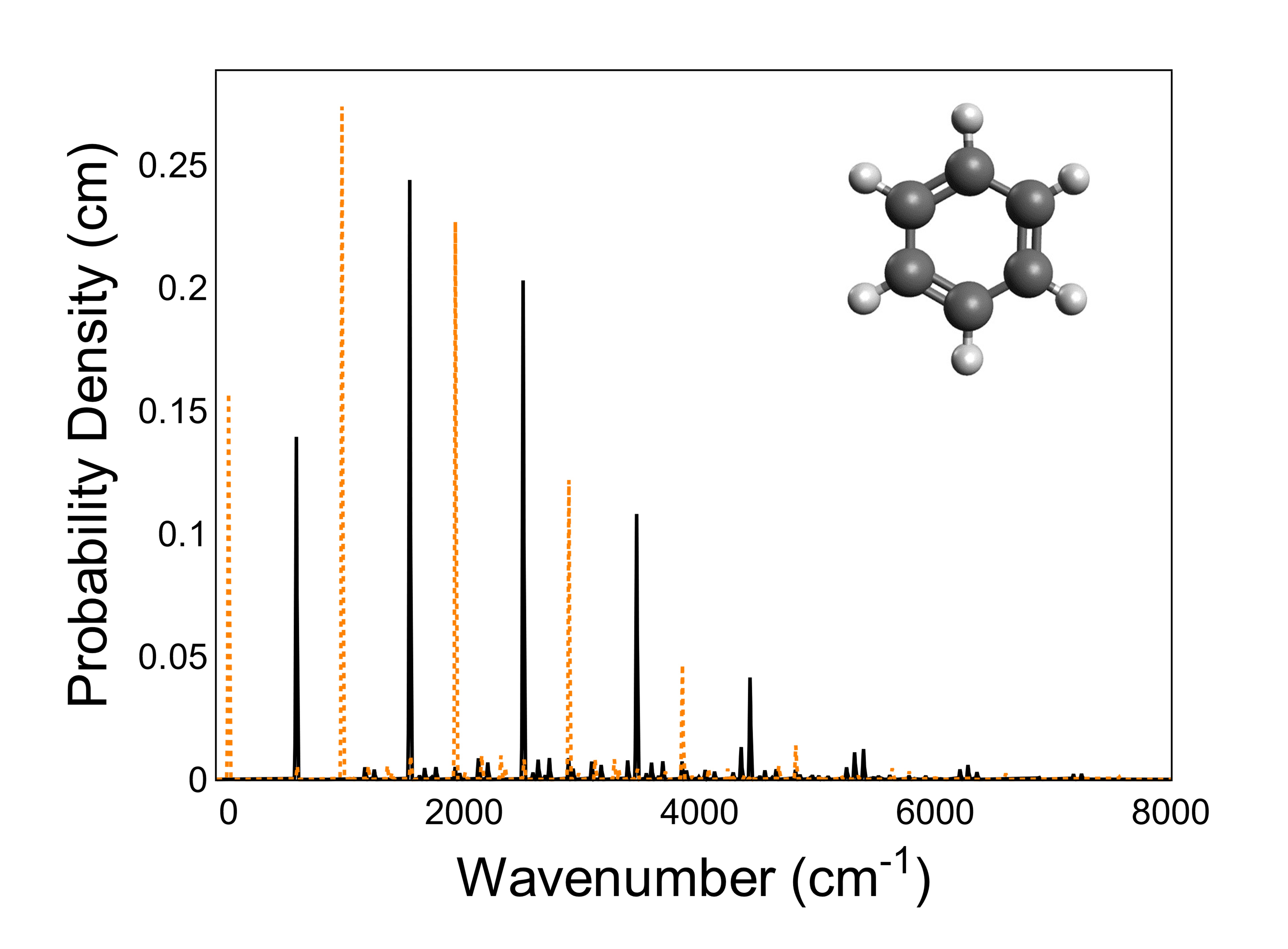
(b)

Figure 3: (a) Exact (black solid line), approximate (orange dotted line), and Franck-Condon (orange dashed line) vibronic spectrum ($\tau=10^{-2}$) of the vibronic transition of benzene (${}^{1}\mathrm{B_{2u}}$–${}^{1}\mathrm{A_{1g}}$) restricted to the $\mathrm{e_{2g}}$ symmetry block. (b) Full vibronic spectrum of Benzene (black solid line) and full vibronic spectrum where the $\mathrm{e_{2g}}$ symmetry block has been deconvoluted (orange dotted line).

IV.2 Second-order Herzberg-Teller expansion

In the previous numerical section, we present an evaluation of our method for linear HT cases. In this subsection, we describe an evaluation of our method for second-order HT expansion with two vibrational modes of benzene belonging to a different symmetry block $\mathrm{e_{1g}}$. By collecting information about the $\mathrm{e_{1g}}$ symmetry block of the vibronic transition of benzene (${}^{1}\mathrm{B_{2u}}$–${}^{1}\mathrm{A_{1g}}$) [50, 51], we created the following model to evaluate the proposed method for the second-order HT expansion. As this transition is Franck-Condon-forbidden ($\mu^{(0)}=0$), it is an excellent candidate to illustrate our method. The molecular parameters are summarized in Table 2.

Table 2: Molecular parameters for three $\mathrm{e_{1g}}$ vibrational modes of benzene. $\bm{\omega}$ and $\bm{\omega^{{}^{\prime}}}$ are the harmonic frequencies of the initial and excited states, respectively, given in $\mathrm{cm}^{-1}$. $\mathbf{U_{\mathrm{D}}}$ is the Duschinsky unitary matrix. The displacement is zero in this case. The elements in $\mathbf{M}$ are given in $\mathrm{D}/({\mathrm{u}^{\tfrac{1}{2}}a_{0}})^{2}$.

Molecule	$\mathbf{M}$	$\bm{\omega}$ ($\mathrm{cm}^{-1}$)	$\bm{\omega^{{}^{\prime}}}$ ($\mathrm{cm}^{-1}$)	$\mathbf{U_{\mathrm{D}}}$
Benzene	$\begin{pmatrix}0&\mu^{(2)}_{1,2}&\mu^{(2)}_{1,2}\\ \mu^{(2)}_{1,2}&\mu^{(2)}_{2,2}&\mu^{(2)}_{2,2}\\ \mu^{(2)}_{1,2}&\mu^{(2)}_{2,2}&-\mu^{(2)}_{2,2}\end{pmatrix}$	$(712.6271,869.5370,869.5370)$	$(482.2731,593.2363,593.2363)$	$\begin{pmatrix}1&0&0\\ 0&0&1\\ 0&1&0\\ \end{pmatrix}$

The transition moment operator is given by

$$\hat{\mu}(\hat{\mathbf{q}})=\hat{\mathbf{q}}^{\mathrm{t}}\bm{\Lambda}\hat{\mathbf{q}},$$ (25)

leading to,

$$f_{\mathbf{m^{{}^{\prime}}}}(\kappa)=\prod^{M}_{j=1}|C_{j,\kappa}|^{2}\left|\bra{\mathbf{m^{{}^{\prime}}}}\hat{U}_{\mathrm{Dok}}\hat{R}(\mathbf{U}^{\mathrm{t}})\hat{S}(\bm{\Xi}_{\kappa})\ket{\mathbf{0}}\right|^{2},$$ (26)

with $C_{j,\kappa}=\tfrac{1}{\sqrt{|s_{j,\kappa}|(1-\kappa d_{j})}}\;\mathrm{and}\;\bm{\Xi}_{\kappa}=\mathrm{diag}\left(\xi_{1,\kappa},\ldots,\xi_{M,\kappa}\right)$ defined in (16).

Here, we used a three-mode model and limited the number of photons per mode to five ($\mathrm{for}\,\tau=10^{-2},\,\sum_{\omega,\,\mathrm{cutoff}=5}P_{\tau}(\omega)\approx 0.9993$). This limitation will not hinder the experiment, as the photon-number-resolving detection scheme developed in [31] could resolve up to $n=16$ Fock states per mode. However, we could recover large portions of the profile with a cutoff of three photons per mode ($\mathrm{for}\,\tau=10^{-2},\,\sum_{\omega,\,\mathrm{cutoff}=3}P_{\tau}(\omega)\approx 0.9872$), leading to a simplified experiment. The results are plotted in Fig. 4.

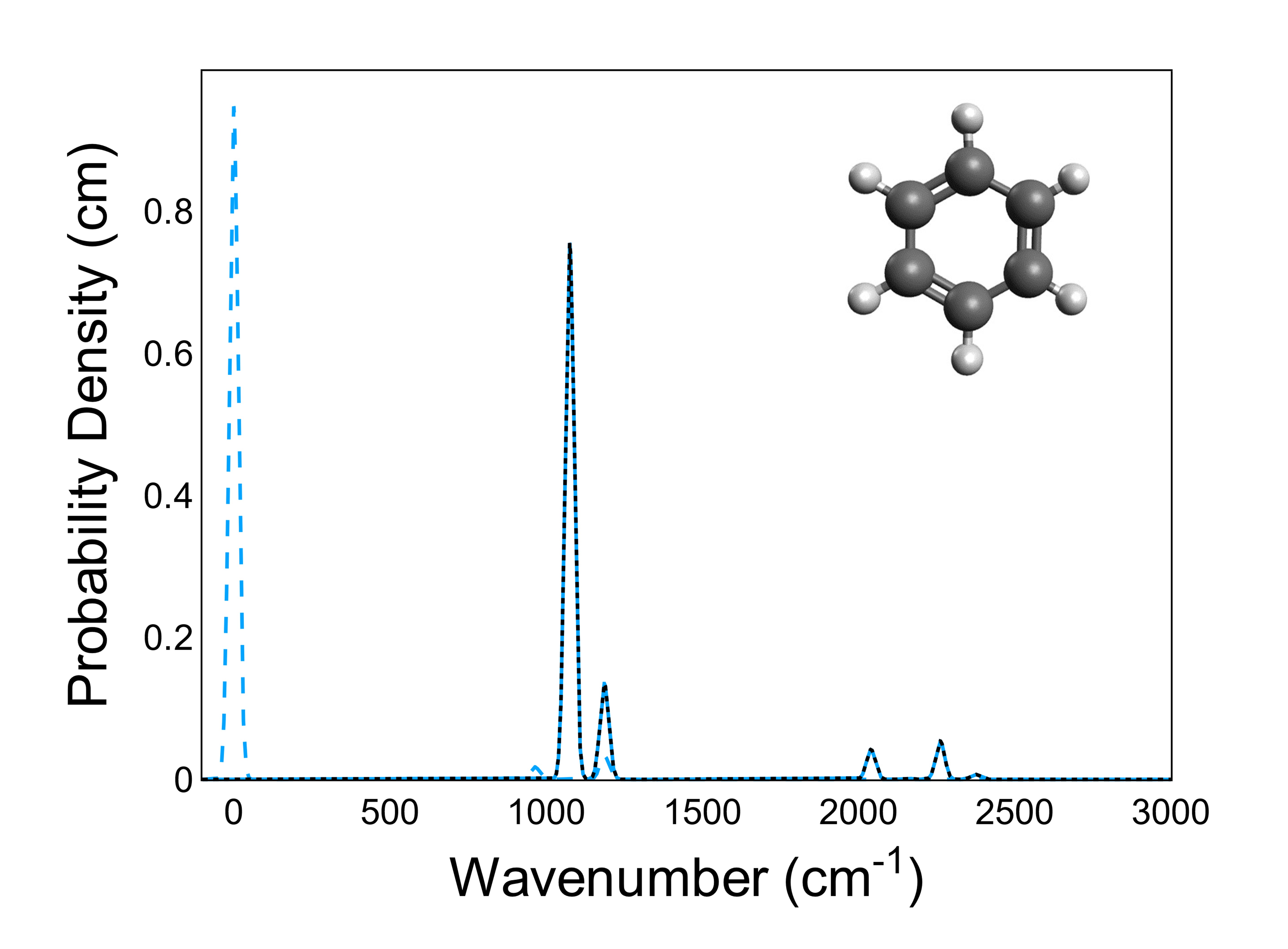
Figure 4: Exact (black solid line), approximate (blue dotted line), and Franck-Condon (blue dashed line) vibronic spectrum ($\tau=10^{-2}$) of the vibronic transition of benzene (${}^{1}\mathrm{B_{2u}}$–${}^{1}\mathrm{A_{1g}}$).

The Duschinsky rotation is an identity matrix (by a proper permutation), and because there is no displacement, we must find a spectrum close to $\hat{U}_{\mathrm{Dok}}\hat{\mu}(\hat{\mathbf{q}})\ket{000}\approx\Lambda_{1,2}(\ket{110}+\ket{101})+\Lambda_{2,2}(\ket{011}+\tfrac{1}{\sqrt{2}}\ket{020}+\tfrac{1}{\sqrt{2}}\ket{002})$. As $\omega^{{}^{\prime}}_{2}=\omega^{{}^{\prime}}_{3}$ (meaning that the permutation does not do anything), we have $\omega_{\ket{110}}=\omega_{\ket{101}}$ and $\omega_{\ket{011}}=\omega_{\ket{020}}=\omega_{\ket{002}}$. We must then obtain a peak at $\omega_{\ket{110}}=\omega^{{}^{\prime}}_{1}+\omega^{{}^{\prime}}_{2}\approx 1.0760\times 10^{3}\,\mathrm{cm}^{-1}$ and another at $\omega_{\ket{011}}=2\omega^{{}^{\prime}}_{2}\approx 1.1860\times 10^{3}\,\mathrm{cm}^{-1}$, with $P(\omega_{\ket{110}})=\tfrac{\Lambda_{1,2}^{2}}{\Lambda_{1,2}^{2}+\Lambda_{2,2}^{2}}\approx 0.8486$ and $P(\omega_{\ket{011}})=\tfrac{\Lambda_{2,2}^{2}}{\Lambda_{1,2}^{2}+\Lambda_{2,2}^{2}}\approx 0.1514$. Peaks at higher wavenumbers come from $\hat{U}_{\mathrm{Dok}}$ and induce a small reduction of the precedent probabilities. Here, we also present the Franck-Condon spectum (dashed blue line in Fig. 4) to compare it with the non-Condon spectra.

Lastly, we analyzed the errors depending on the size of the parameter $\tau$ (see Fig. 5). Ideally, the error behaves quadratically with $\tau$. As indicated in Fig. 5, almost all cases exhibited ideal behavior. However, one error of benzene (second-order HT expansion at $\tau=10^{-2}$) deviated from the expected value. To examine the cause, we consider an effective parameter $\tau_{\mathrm{eff}}$. For benzene, $\hat{\mu}=\hat{\mathbf{q}}^{\mathrm{t}}\bm{\Lambda}\hat{\mathbf{q}}$ where all the parameters in $\bm{\Lambda}$ are on the order of $10^{-3}$ (after conversion). We can then rewrite $\hat{\mu}=10^{-3}\hat{\mu}_{\mathrm{eff}}$, which leads to rescaling the expansion parameter $\tau$ effectively, that is, $\tau_{\mathrm{eff}}=10^{-3}\tau$. Therefore, taking a small value of $\tau$ in the expansion, we would encounter a numerical rounding-off error earlier than in the linear case.

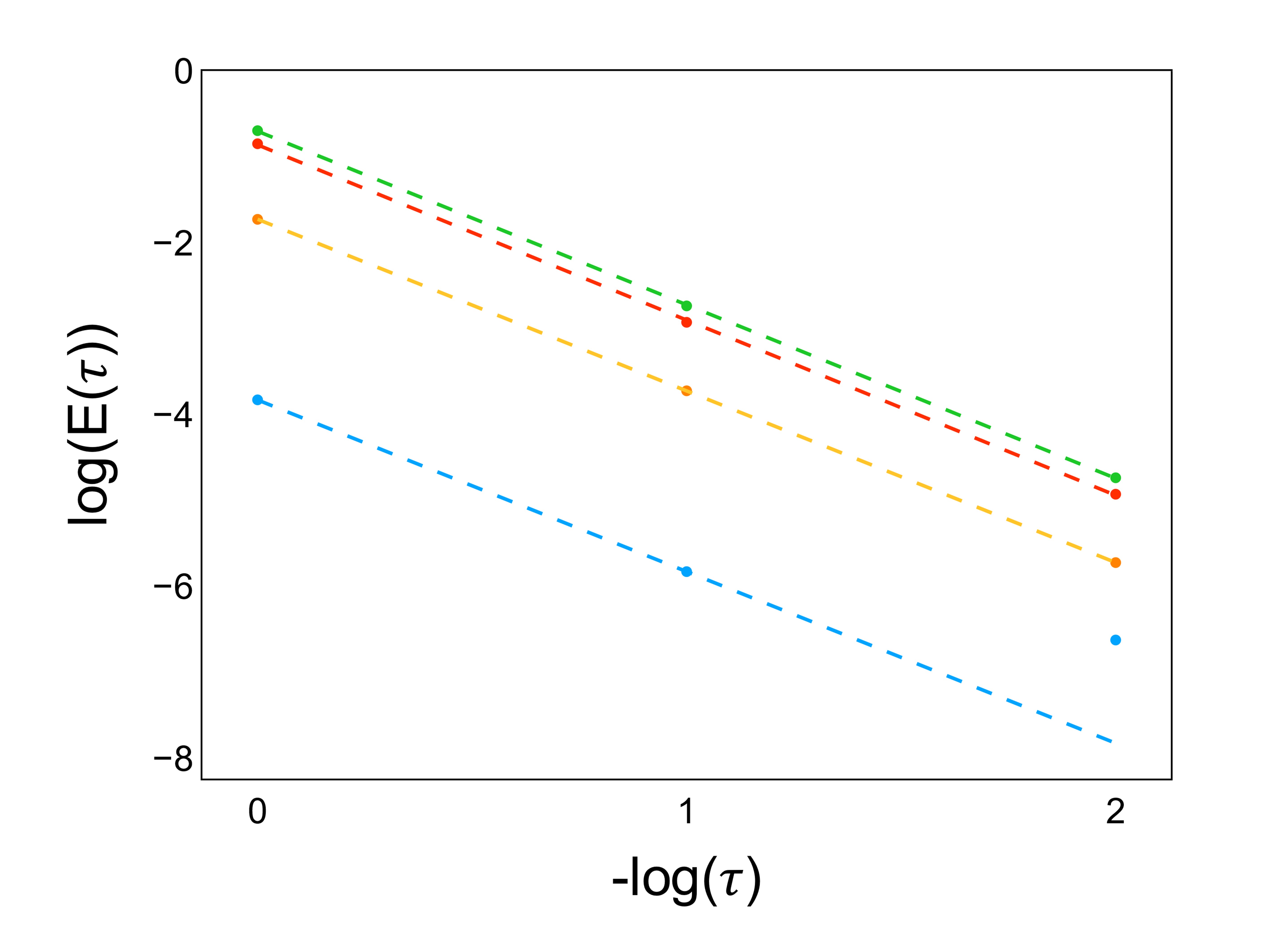
Figure 5: Error between exact and approximate profiles for different values of $\tau$ ($\mathrm{E}(\tau)=|P_{\mathrm{exact}}-P_{\tau}|$). The red dashes represent the error for naphthalene, the green dashes the error for phenanthrene, and the yellow and blue dashes represent the first-order and second-order HT transion of benzene, respectively. The slopes of the lines are close to -2, which is expected from the method developed in this paper.

V Conclusion and outlook

Without consideration of practical applications, boson sampling was introduced as an easily implementable device whose computational power can surpass that of classical computers. However, the proposal by Huh et al. [12] revealed that boson sampling can also be useful for quantum simulation. Our work generalizes the aforementioned study by simulating more complex molecular processes beyond the Condon regime, thereby increasing the number of practical applications of boson sampling [52]. The non-Condon profile was approximated with linear optics simply by using a linear combination of Gaussian boson samplers that we introduced. We note here that our new development is not just an extension of the theoretical proposal of Huh and coworkers [12]. The method opened a new way to approximate non-unitary operations in a linear optical network that it can be generalized to arbitrary non-unitary operators and digital quantum simulations. Our technique can potentially enable the extraction of relevant molecular properties that exhibit strong non-Condon effects without resorting to the use of digital quantum computers for the Condon case [14, 21, 27].

Focusing on small molecules to motivate experimental implementations, we evaluated our method for both linear and quadratic HT expansions through numerical examples. In each case, we successfully simulated the non-Condon profiles with a small error. However, because we studied probability densities, we did not consider errors due to sampling. In fact, we had infinite precision in the estimation of the probabilities. In an experiment in which the profile is reconstructed by sampling from the approximated probability density, there will be errors due to the finite number of samples considered.

Our work can be extended to other types of vibronic transitions such as resonance Raman spectroscopy [53], internal conversion [54], and intersystem crossing [55], as all of these are related by the computation of a non-Condon integral to evaluate the probability of a transition. Furthermore, we can also generalize the work performed in [14] for the quantum circuit model to include non-Condon effects based on the current development or to describe the non-adiabatic molecular quantum dynamics [56]. Finally, we can reuse the concepts developed in this paper to improve current classical algorithms used for molecular vibronic spectroscopy in the non-Condon case; for example, we can combine the current approach with the time-dependent method [11, 38].

Appendix A Computation of the normalization constant

We start from the normalization condition,

$$1=\sum_{\omega=0}^{\infty}P(\omega)=\frac{1}{\mathcal{N}}\sum_{r=x,y,z}\sum_{\omega=0}^{\infty}\sum_{\mathbf{m^{{}^{\prime}}}=\mathbf{0}}^{\bm{\infty}}|\langle\mathbf{m^{{}^{\prime}}}|\hat{U}_{\mathrm{Dok}}\hat{\mu}_{r}|\mathbf{0}\rangle|^{2}\delta(\omega-\mathbf{m^{{}^{\prime}}}\cdot\bm{\omega}^{\prime}).$$ (27)

But,

$$\sum_{\omega=0}^{\infty}\sum_{\mathbf{m^{{}^{\prime}}}=\mathbf{0}}^{\bm{\infty}}|\langle\mathbf{m^{{}^{\prime}}}|\hat{U}_{\mathrm{Dok}}\hat{\mu}_{r}|\mathbf{0}\rangle|^{2}\delta(\omega-\mathbf{m^{{}^{\prime}}}\cdot\bm{\omega}^{\prime}) =\sum_{\omega=0}^{\infty}\sum_{\mathbf{m^{{}^{\prime}}}=\mathbf{0}}^{\bm{\infty}}\bra{\mathbf{0}}\hat{\mu}_{r}^{\dagger}\hat{U}_{\mathrm{Dok}}^{\dagger}\ket{\mathbf{m^{{}^{\prime}}}}\bra{\mathbf{m^{{}^{\prime}}}}\hat{U}_{\mathrm{Dok}}\hat{\mu}_{r}\ket{\mathbf{0}}\delta(\omega-\mathbf{m^{{}^{\prime}}}\cdot\bm{\omega}^{\prime})$$

$$=\bra{\mathbf{0}}\hat{\mu}_{r}^{\dagger}\hat{U}_{\mathrm{Dok}}^{\dagger}\left(\sum_{\omega=0}^{\infty}\sum_{\mathbf{m^{{}^{\prime}}}=\mathbf{0}}^{\bm{\infty}}\ket{\mathbf{m^{{}^{\prime}}}}\bra{\mathbf{m^{{}^{\prime}}}}\delta(\omega-\mathbf{m^{{}^{\prime}}}\cdot\bm{\omega}^{\prime})\right)\hat{U}_{\mathrm{Dok}}\hat{\mu}_{r}\ket{\mathbf{0}}.$$ (28)

And,

$$\sum_{\omega=0}^{\infty}\sum_{\mathbf{m^{{}^{\prime}}}=\mathbf{0}}^{\bm{\infty}}\ket{\mathbf{m^{{}^{\prime}}}}\bra{\mathbf{m^{{}^{\prime}}}}\delta(\omega-\mathbf{m^{{}^{\prime}}}\cdot\bm{\omega}^{\prime}) =\sum_{\mathbf{m^{{}^{\prime}}}=\mathbf{0}}^{\bm{\infty}}\ket{\mathbf{m^{{}^{\prime}}}}\bra{\mathbf{m^{{}^{\prime}}}}\left(\sum_{\omega=0}^{\infty}\delta(\omega-\mathbf{m^{{}^{\prime}}}\cdot\bm{\omega}^{\prime})\right)$$

$$=\sum_{\mathbf{m^{{}^{\prime}}}=\mathbf{0}}^{\bm{\infty}}\ket{\mathbf{m^{{}^{\prime}}}}\bra{\mathbf{m^{{}^{\prime}}}}$$

$$=\mathcal{I}.$$ (29)

Moreover $\hat{\mu}_{r}=\hat{\mu}_{r}^{\dagger}$ which leads to,

$$\mathcal{N}=\sum_{r=x,y,z}\mathcal{N}_{r}=\sum_{r=x,y,z}\bra{\mathbf{0}}\hat{\mu}_{r}\hat{U}_{\mathrm{Dok}}^{\dagger}\hat{U}_{\mathrm{Dok}}\hat{\mu}_{r}\ket{\mathbf{0}}=\sum_{r=x,y,z}\bra{\mathbf{0}}\hat{\mu}_{r}^{2}\ket{\mathbf{0}}$$ (30)

as $\hat{U}_{\mathrm{Dok}}$ is a unitary operator. We derive the normalization factor for the second-order expansion, the first-order one being found by taking $\bm{\Lambda}_{r}=\mathbf{0}$. We have, $\hat{\mu}_{r}(\mathbf{\hat{q}})=\mu_{r}^{(0)}+\sum_{j=1}^{M}\lambda_{r,j}\hat{q}_{r,j}+\sum_{j,k=1}^{M}[\bm{\Lambda}_{r}]_{j,k}\hat{q}_{r,j}\hat{q}_{r,k}$. When considering the overlap $\bra{\mathbf{0}}\hat{\mu}_{r}^{2}\ket{\mathbf{0}}$, the terms of the type $\bra{\bm{0}}\hat{q}_{r,j}\hat{q}_{r,k}\ket{\bm{0}}$ for $j\neq k$, or $\bra{\bm{0}}\hat{q}_{r,i}\hat{q}_{r,j}\hat{q}_{r,k}\hat{q}_{r,l}\ket{\bm{0}}$ for $\{k,l\}$ not a permutation of $\{i,j\}$ vanish as we get the overlap between two orthogonal basis vectors. Finally, we get,

$$\mathcal{N}_{2} =\sum_{r=x,y,z}\mathcal{N}_{r,2}$$

$$=\sum_{r=x,y,z}\left((\mu_{r}^{(0)})^{2}+\tfrac{1}{2}\sum_{j=1}^{M}\lambda_{r,j}^{2}+\mu_{r}^{(0)}\sum_{j=1}^{M}[\bm{\Lambda}_{r}]_{j,j}+\tfrac{1}{4}\sum_{\begin{subarray}{c}j,k=1\\ j\neq k\end{subarray}}^{M}[\bm{\Lambda}_{r}]_{j,j}[\bm{\Lambda}_{r}]_{k,k}+\tfrac{1}{2}\sum_{\begin{subarray}{c}j,k=1\\ j\neq k\end{subarray}}^{M}[\bm{\Lambda}_{r}]_{j,k}^{2}+\tfrac{3}{4}\sum_{j=1}^{M}[\bm{\Lambda}_{r}]_{j,j}^{2}\right).$$ (31)

Appendix B Derivation of $\exp(\kappa\hat{\mu})|\mathbf{0}\rangle$

If $\kappa$ was purely imaginary, then $\exp(\kappa\hat{\mu})$ would be a unitary (as $\hat{\mu}$ is Hermitian) and it would be straightforward to implement the linear optical setup. However, it is necessary to generalize the application of the operator for $\kappa$ can be a real number. Therefore, we have,

$$\exp(\kappa\hat{\mu})|\mathbf{0}\rangle =\hat{R}(\mathbf{U}^{\mathrm{t}})\exp(\kappa(\mu^{(0)}+\mathbf{b}^{\mathrm{t}}\hat{\mathbf{q}}+\hat{\mathbf{q}}^{\mathrm{t}}\mathbf{D}\hat{\mathbf{q}}))|\mathbf{0}\rangle$$

$$=\exp(\kappa\mu^{(0)})\hat{R}(\mathbf{U}^{\mathrm{t}})\bigotimes_{j=1}^{M}\exp(\kappa b_{j}\hat{q}_{j}+\kappa d_{j}\hat{q}_{j}^{2})|0\rangle_{j}.$$

Now, we need to find the expression of $\exp(\kappa b_{j}\hat{q}_{j}+\kappa d_{j}\hat{q}_{j}^{2})|0\rangle_{j}=\exp(\kappa b_{j}\hat{q}_{j})\exp(\kappa d_{j}\hat{q}_{j}^{2})|0\rangle_{j}$ (as $[\hat{q}_{j},\hat{q}_{j}^{2}]=0$) in terms of Gaussian operators. On the one hand [46],

$$\exp(\kappa d_{j}\hat{q}_{j}^{2})\ket{0}_{j} =\int_{-\infty}^{\infty}\mathrm{d}q_{j}\exp(\kappa d_{j}q_{j}^{2})|q_{j}\rangle\langle q_{j}|\ket{0}_{j}$$

$$=\int_{-\infty}^{\infty}\frac{\mathrm{d}q_{j}}{\sqrt{\pi}}\exp(\kappa d_{j}q_{j}^{2}):\exp(-(q_{j}-\hat{q}_{j})^{2}):\ket{0}_{j}$$

$$=\int_{-\infty}^{\infty}\frac{\mathrm{d}q_{j}}{\sqrt{\pi}}:\exp\left(-(1-\kappa d_{j})q_{j}^{2}+2\hat{q}_{j}q_{j}-\hat{q}_{j}^{2}\right):\ket{0}_{j}$$

$$=\frac{1}{\sqrt{1-\kappa d_{j}}}:\exp\left(\frac{\kappa d_{j}}{1-\kappa d_{j}}\hat{q}_{j}^{2}\right):\ket{0}_{j}$$

$$=\frac{1}{\sqrt{1-\kappa d_{j}}}\exp\left(\frac{1}{2}\frac{\kappa d_{j}}{1-\kappa d_{j}}\hat{a}_{j}^{\dagger 2}\right)\ket{0}_{j},$$ (33)

where : : denotes normal ordering. On the other hand, the squeezing operator can be arranged in a normal ordered form,

$$\hat{S}_{j}(\xi_{j})\ket{0}_{j} =\exp(\tfrac{1}{2}(\xi_{j}\hat{a}_{j}^{\dagger 2}-\xi_{j}^{*}\hat{a}_{j}^{2}))\ket{0}_{j}$$

$$=|s_{j}|^{\tfrac{1}{2}}\exp(\tfrac{1}{2}t_{j}\hat{a}_{j}^{\dagger 2}):\exp((s_{j}-1)\hat{a}_{j}^{\dagger}\hat{a}_{j}):\exp(-\tfrac{1}{2}t_{j}\hat{a}_{j}^{2})\ket{0}_{j}$$

$$=|s_{j}|^{\tfrac{1}{2}}\exp(\tfrac{1}{2}t_{j}\hat{a}_{j}^{\dagger 2})\ket{0}_{j},$$ (34)

where $\xi_{j}=r_{j}\exp(\mathrm{i}\theta_{j})$, $t_{j}=\tanh(r_{j})\exp(\mathrm{i}\theta_{j})$, $s_{j}=\mathrm{sech}(r_{j})$. Then by identification,

$$\exp(\kappa d_{j}\hat{q}_{j}^{2})\ket{0}_{j}=\frac{1}{\sqrt{|s_{j,\kappa}|(1-\kappa d_{j})}}\hat{S}_{j}(\xi_{j,\kappa})\ket{0}_{j}.$$ (35)

with $t_{j,\kappa}=\tfrac{\kappa d_{j}}{1-\kappa d_{j}}$. $r_{j,\kappa},\theta_{j,\kappa}$ and $\xi_{j,\kappa}$ stem from $t_{j,\kappa}$. Then,

$$\exp(\kappa b_{j}\hat{q}_{j}+\kappa d_{j}\hat{q}_{j}^{2})\ket{0}_{j} =\exp(\kappa b_{j}\hat{q}_{j})\exp(\kappa d_{j}\hat{q}_{j}^{2})\ket{0}_{j}$$

$$=\frac{1}{\sqrt{|s_{j,\kappa}|(1-\kappa d_{j})}}\exp(\kappa b_{j}\hat{q}_{j})\hat{S}_{j}(\xi_{j,\kappa})\ket{0}_{j}$$ (36)

By using the formulas $\exp(A)\exp(B)=\exp(B)\exp(A)\exp([A,B])$ and $\exp(A+B)=\exp(A)\exp(B)\exp(-\tfrac{1}{2}[A,B])$, we derive the final expression of $\exp(\kappa\hat{\mu})\ket{\mathbf{0}}$,

$$\exp(\kappa b_{j}\hat{q}_{j}+\kappa d_{j}\hat{q}_{j}^{2})\ket{0}_{j}$$

$$=\exp(\kappa b_{j}\hat{q}_{j})\exp(\kappa d_{j}\hat{q}_{j}^{2})|0\rangle_{j}$$

$$=\frac{1}{\sqrt{|s_{j,\kappa}|(1-\kappa d_{j})}}\exp\left(\frac{(\kappa b_{j})^{2}}{4}\right)\exp\left(\frac{\kappa b_{j}}{\sqrt{2}}\hat{a}_{j}^{\dagger}\right)\exp\left(\frac{\kappa b_{j}}{\sqrt{2}}\hat{a}_{j}\right)\hat{S}_{j}(\xi_{j,\kappa})\ket{0}_{j}$$

$$=\frac{1}{\sqrt{|s_{j,\kappa}|(1-\kappa d_{j})}}\exp\left(\frac{(\kappa b_{j})^{2}}{4}\right)\exp\left(\frac{\kappa b_{j}}{\sqrt{2}}\hat{a}_{j}^{\dagger}\right)\hat{S}_{j}(\xi_{j,\kappa})\exp\left(\frac{\kappa b_{j}}{\sqrt{2}}\hat{a}_{j}\right)\exp\left(\frac{\kappa b_{j}\xi_{j,\kappa}}{\sqrt{2}}\hat{a}_{j}^{\dagger}\right)\ket{0}_{j}$$

$$=\frac{1}{\sqrt{|s_{j,\kappa}|(1-\kappa d_{j})}}\exp\left(\frac{(\kappa b_{j})^{2}}{4}\right)\hat{S}_{j}(\xi_{j,\kappa})\exp\left(\frac{\kappa b_{j}}{\sqrt{2}}\hat{a}_{j}^{\dagger}\right)\exp\left(\frac{\kappa b_{j}}{\sqrt{2}}(1+\xi_{j,\kappa}^{*})\hat{a}_{j}\right)\exp\left(\frac{\kappa b_{j}\xi_{j,\kappa}}{\sqrt{2}}\hat{a}_{j}^{\dagger}\right)\ket{0}_{j}$$

$$=\frac{1}{\sqrt{|s_{j,\kappa}|(1-\kappa d_{j})}}\exp\left(\frac{(\kappa b_{j})^{2}}{4}+\frac{(\kappa b_{j})^{2}}{2}(1+\xi_{j,\kappa}^{*})\xi_{j,\kappa}\right)\hat{S}_{j}(\xi_{j,\kappa})\exp\left(\frac{\kappa b_{j}}{\sqrt{2}}(1+\xi_{j,\kappa})\hat{a}_{j}^{\dagger}\right)\exp\left(\frac{\kappa b_{j}}{\sqrt{2}}(1+\xi_{j,\kappa}^{*})\hat{a}_{j}\right)\ket{0}_{j}.$$

However, $\exp\left(\tfrac{\kappa b_{j}}{\sqrt{2}}(1+\xi_{j,\kappa}^{*})\hat{a}_{j}\right)\ket{0}_{j}=\ket{0}_{j}$ because $\hat{a}_{j}\ket{0}_{j}=0$ and,

$$\exp\left(\frac{\kappa b_{j}}{\sqrt{2}}(1+\xi_{j,\kappa})\hat{a}_{j}^{\dagger}\right)\ket{0}_{j}$$

$$=\exp\left(\frac{\kappa b_{j}}{\sqrt{2}}(1+\xi_{j,\kappa})\hat{a}_{j}^{\dagger}\right)\exp\left(\left(\frac{\kappa b_{j}}{\sqrt{2}}(1+\xi_{j,\kappa})\right)^{*}\hat{a}_{j}\right)\ket{0}_{j}$$

$$=\exp\left(\frac{|\kappa b_{j}(1+\xi_{j,\kappa})|^{2}}{4}\right)\hat{D}_{j}\left(\frac{\kappa b_{j}}{\sqrt{2}}(1+\xi_{j,\kappa})\right)\ket{0}_{j},$$ (38)

which leads to,

$$\exp(\kappa b_{j}\hat{q}_{j}+\kappa d_{j}\hat{q}_{j}^{2})\ket{0}_{j}$$

$$=\frac{1}{\sqrt{|s_{j,\kappa}|(1-\kappa d_{j})}}\exp\left(\frac{(\kappa b_{j})^{2}}{4}+\frac{(\kappa b_{j})^{2}}{2}(1+\xi_{j,\kappa}^{*})\xi_{j,\kappa}+\frac{|\kappa b_{j}(1+\xi_{j,\kappa})|^{2}}{4}\right)\hat{S}_{j}(\xi_{j,\kappa})\hat{D}_{j}\left(\frac{\kappa b_{j}(1+\xi_{j,\kappa})}{\sqrt{2}}\right)\ket{0}_{j}$$

$$=C_{j,\kappa}\hat{S}_{j}(\xi_{j,\kappa})\hat{D}_{j}\left(\alpha_{j,\kappa}\right)\ket{0}_{j},$$ (39)

where $t_{j,\kappa}=\tfrac{\kappa d_{j}}{1-\kappa d_{j}}$, $r_{j,\kappa}=|t_{j,\kappa}|$, $\theta_{j,\kappa}=\arg(t_{j,\kappa})$, $\xi_{j,\kappa}=\mathrm{arctanh}(r_{j,\kappa})\exp(i\theta_{j,\kappa})$, $s_{j,\kappa}=\mathrm{sech}(|\xi_{j,\kappa}|)$, $C_{j,\kappa}=\tfrac{1}{\sqrt{|s_{j,\kappa}|(1-\kappa d_{j})}}\exp\left(\tfrac{(\kappa b_{j})^{2}}{4}+\tfrac{(\kappa b_{j})^{2}}{2}(1+\xi_{j,\kappa}^{*})\xi_{j,\kappa}+\tfrac{|\kappa b_{j}(1+\xi_{j,\kappa})|^{2}}{4}\right)$ and $\alpha_{j,\kappa}=\tfrac{\kappa b_{j}}{\sqrt{2}}(1+\xi_{j,\kappa})$.

Appendix C Bloch-Messiah decomposition

Initially we have,

$$f_{\mathbf{m^{{}^{\prime}}}}(\kappa)=\exp(2\kappa\mu^{(0)})\prod^{M}_{j=1}|C_{j,\kappa}|^{2}\left|\bra{\mathbf{m^{{}^{\prime}}}}\hat{R}(\mathbf{U_{2}})\hat{S}(\mathbf{\ln(L)})\hat{R}(\mathbf{U_{1}})\hat{D}(\bm{\beta})\hat{R}(\mathbf{U}^{\mathrm{t}})\hat{S}(\bm{\Xi}_{\kappa})\hat{D}(\bm{\alpha}_{\kappa})\ket{\mathbf{0}}\right|^{2}$$ (40)

However, by using the Bloch-Messiah decomposition we can rewrite [57, 58] the Gaussian operator $\hat{R}(\mathbf{U_{2}})\hat{S}(\mathbf{\ln(L)})\hat{R}(\mathbf{U_{1}})\hat{D}(\bm{\beta})\hat{R}(\mathbf{U}^{\mathrm{t}})\hat{S}(\bm{\Xi}_{\kappa})\hat{D}(\bm{\alpha}_{\kappa})$ in a simpler form, which will lead to a simpler experimental realization. Let $\hat{O}_{\kappa}=\hat{R}(\mathbf{U_{2}})\hat{S}(\mathbf{\ln(L)})\hat{R}(\mathbf{U_{1}})\hat{D}(\bm{\beta})\hat{R}(\mathbf{U}^{\mathrm{t}})\hat{S}(\bm{\Xi}_{\kappa})\hat{D}(\bm{\alpha}_{\kappa})$. The first step to find its Bloch-Messiah decomposition is to find the Bogoliubov operators corresponding to the action of $\hat{O}_{\kappa}$ on the creation operator. In other words, we need to find $\mathbf{X}_{\kappa},\mathbf{Y}_{\kappa}$ and $\mathbf{z}_{\kappa}$ such that,

$$\hat{\mathbf{a}}^{{}^{\prime}\dagger}=\hat{O}_{\kappa}^{\dagger}\hat{\mathbf{a}}^{\dagger}\hat{O}_{\kappa}=\mathbf{X}_{\kappa}\hat{\mathbf{a}}+\mathbf{Y}_{\kappa}\hat{\mathbf{a}}^{\dagger}+\mathbf{z}_{\kappa}.$$ (41)

Then, by taking the singular value decomposition $\mathbf{X}_{\kappa}=\mathbf{V}_{\kappa}\mathrm{sinh}(\bm{\Sigma}_{\kappa})\mathbf{W}_{\kappa}^{\mathrm{t}},\mathbf{Y}_{\kappa}=\mathbf{V}_{\kappa}\mathrm{cosh}(\bm{\Sigma}_{\kappa})\mathbf{W}_{\kappa}^{\dagger}$, we will have,

$$\hat{O}_{\kappa}=\hat{D}(\mathbf{z}_{\kappa})\hat{R}(\mathbf{V}_{\kappa})\hat{S}(\bm{\Sigma}_{\kappa})\hat{R}(\mathbf{W}_{\kappa})^{\dagger},$$ (42)

We remind here the actions of the multimode Gaussian operators on the ladder operators,

$$\hat{S}(\bm{\Xi})^{\dagger}\hat{\mathbf{a}}\hat{S}(\bm{\Xi}) =\mathrm{cosh}(\bm{\Xi})\hat{\mathbf{a}}+\mathrm{sinh}(\bm{\Xi})\hat{\mathbf{a}}^{\dagger},$$ (43)

$$\hat{D}(\bm{\alpha})^{\dagger}\hat{\mathbf{a}}\hat{D}(\bm{\alpha}) =\hat{\mathbf{a}}+\bm{\alpha},$$ (44)

$$\hat{R}(\mathbf{U})^{\dagger}\hat{\mathbf{a}}\hat{R}(\mathbf{U}) =\mathbf{U}\hat{\mathbf{a}}.$$ (45)

By applying these rules sequentially we get,

$$\hat{\mathbf{a}}^{{}^{\prime}\dagger} =\hat{O}_{\kappa}^{\dagger}\hat{\mathbf{a}}^{\dagger}\hat{O}_{\kappa}$$

$$=(\hat{R}({\mathbf{U_{2}}})\hat{S}(\mathbf{\ln(L)})\hat{R}(\mathbf{U}_{1})\hat{D}(\bm{\beta})\hat{R}(\mathbf{U}^{\mathrm{t}})\hat{S}(\bm{\Xi}_{\kappa})\hat{D}(\bm{\alpha}))^{\dagger}\left(\hat{\mathbf{a}}^{\dagger}\right)(\hat{R}({\mathbf{U_{2}}})\hat{S}(\mathbf{\ln(L)})\hat{R}(\mathbf{U}_{1})\hat{D}(\bm{\beta})\hat{R}(\mathbf{U}^{\mathrm{t}})\hat{S}(\bm{\Xi}_{\kappa})\hat{D}(\bm{\alpha}))$$

$$=(\hat{S}(\mathbf{\ln(L)})\hat{R}(\mathbf{U}_{1})\hat{D}(\bm{\beta})\hat{R}(\mathbf{U}^{\mathrm{t}})\hat{S}(\bm{\Xi}_{\kappa})\hat{D}(\bm{\alpha}))^{\dagger}\left(\mathbf{U_{2}}\hat{\mathbf{a}}^{\dagger}\right)(\hat{S}(\mathbf{\ln(L)})\hat{R}(\mathbf{U}_{1})\hat{D}(\bm{\beta})\hat{R}(\mathbf{U}^{\mathrm{t}})\hat{S}(\bm{\Xi}_{\kappa})\hat{D}(\bm{\alpha}))$$

$$=(\hat{R}(\mathbf{U}_{1})\hat{D}(\bm{\beta})\hat{R}(\mathbf{U}^{\mathrm{t}})\hat{S}(\bm{\Xi}_{\kappa})\hat{D}(\bm{\alpha}))^{\dagger}\left(\mathbf{U_{2}}\mathrm{cosh}(\mathbf{\ln(L)})\hat{\mathbf{a}}^{\dagger}+\mathbf{U_{2}}\mathrm{sinh}(\mathbf{\ln(L)})\hat{\mathbf{a}}\right)(\hat{R}(\mathbf{U}_{1})\hat{D}(\bm{\beta})\hat{R}(\mathbf{U}^{\mathrm{t}})\hat{S}(\bm{\Xi}_{\kappa})\hat{D}(\bm{\alpha}))$$

$$=(\hat{D}(\bm{\beta})\hat{R}(\mathbf{U}^{\mathrm{t}})\hat{S}(\bm{\Xi}_{\kappa})\hat{D}(\bm{\alpha}))^{\dagger}\left(\mathbf{U_{2}}\mathrm{cosh}(\mathbf{\ln(L)})\mathbf{U_{1}}\hat{\mathbf{a}}^{\dagger}+\mathbf{U_{2}}\mathrm{cosh}(\mathbf{\ln(L)})\mathbf{U_{1}}\hat{\mathbf{a}}\right)(\hat{D}(\bm{\beta})\hat{R}(\mathbf{U}^{\mathrm{t}})\hat{S}(\bm{\Xi}_{\kappa})\hat{D}(\bm{\alpha}))$$

$$=(\hat{R}(\mathbf{U}^{\mathrm{t}})\hat{S}(\bm{\Xi}_{\kappa})\hat{D}(\bm{\alpha}))^{\dagger}\left(\mathbf{U_{2}}\mathrm{cosh}(\mathbf{\ln(L)})\mathbf{U_{1}}\hat{\mathbf{a}}^{\dagger}+\mathbf{U_{2}}\mathrm{sinh}(\mathbf{\ln(L)})\mathbf{U_{1}}\hat{\mathbf{a}}+\mathbf{U_{2}}\exp(\mathbf{\ln(L)})\mathbf{U_{1}}\bm{\beta}\right)(\hat{R}(\mathbf{U}^{\mathrm{t}})\hat{S}(\bm{\Xi}_{\kappa})\hat{D}(\bm{\alpha}))$$

$$=(\hat{S}(\bm{\Xi}_{\kappa})\hat{D}(\bm{\alpha}))^{\dagger}\left(\mathbf{U_{2}}\mathrm{cosh}(\mathbf{\ln(L)})\mathbf{U_{1}}\mathbf{U}^{\mathrm{t}}\hat{\mathbf{a}}^{\dagger}+\mathbf{U_{2}}\mathrm{sinh}(\mathbf{\ln(L)})\mathbf{U_{1}}\mathbf{U}^{\mathrm{t}}\hat{\mathbf{a}}+\mathbf{U_{2}}\mathbf{L}\mathbf{U_{1}}\bm{\beta}\right)(\hat{S}(\bm{\Xi}_{\kappa})\hat{D}(\bm{\alpha}))$$

$$=\hat{D}(\bm{\alpha})^{\dagger}([\mathbf{U_{2}}\mathrm{cosh}(\mathbf{\ln(L)})\mathbf{U_{1}}\mathbf{U}^{\mathrm{t}}\mathrm{cosh}(\bm{\Xi}_{\kappa})+\mathbf{U_{2}}\mathrm{sinh}(\mathbf{\ln(L)})\mathbf{U_{1}}\mathbf{U}^{\mathrm{t}}\mathrm{sinh}(\bm{\Xi}_{\kappa})]\hat{\mathbf{a}}^{\dagger}$$

$$+[\mathbf{U_{2}}\mathrm{sinh}(\mathbf{\ln(L)})\mathbf{U_{1}}\mathbf{U}^{\mathrm{t}}\mathrm{cosh}(\bm{\Xi}_{\kappa})+\mathbf{U_{2}}\mathrm{cosh}(\mathbf{\ln(L)})\mathbf{U_{1}}\mathbf{U}^{\mathrm{t}}\mathrm{sinh}(\bm{\Xi}_{\kappa})]\hat{\mathbf{a}}+\mathbf{U_{2}}\mathbf{L}\mathbf{U_{1}}\bm{\beta})\hat{D}(\bm{\alpha})$$

$$=\left[\mathbf{U_{2}}\mathrm{cosh}(\mathbf{\ln(L)})\mathbf{U_{1}}\mathbf{U}^{\mathrm{t}}\mathrm{cosh}(\bm{\Xi}_{\kappa})+\mathbf{U_{2}}\mathrm{sinh}(\mathbf{\ln(L)})\mathbf{U_{1}}\mathbf{U}^{\mathrm{t}}\mathrm{sinh}(\bm{\Xi}_{\kappa})\right]\hat{\mathbf{a}}^{\dagger}$$

$$+\left[\mathbf{U_{2}}\mathrm{sinh}(\mathbf{\ln(L)})\mathbf{U_{1}}\mathbf{U}^{\mathrm{t}}\mathrm{cosh}(\bm{\Xi}_{\kappa})+\mathbf{U_{2}}\mathrm{cosh}(\mathbf{\ln(L)})\mathbf{U_{1}}\mathbf{U}^{\mathrm{t}}\mathrm{sinh}(\bm{\Xi}_{\kappa})\right]\hat{\mathbf{a}}$$

$$+[\mathbf{U_{2}}\mathrm{cosh}(\mathbf{\ln(L)})\mathbf{U_{1}}\mathbf{U}^{\mathrm{t}}\mathrm{cosh}(\bm{\Xi}_{\kappa})+\mathbf{U_{2}}\mathrm{sinh}(\mathbf{\ln(L)})\mathbf{U_{1}}\mathbf{U}^{\mathrm{t}}\mathrm{sinh}(\bm{\Xi}_{\kappa})$$

$$+\mathbf{U_{2}}\mathrm{sinh}(\mathbf{\ln(L)})\mathbf{U_{1}}\mathbf{U}^{\mathrm{t}}\mathrm{cosh}(\bm{\Xi}_{\kappa})+\mathbf{U_{2}}\mathrm{cosh}(\mathbf{\ln(L)})\mathbf{U_{1}}\mathbf{U}^{\mathrm{t}}\mathrm{sinh}(\bm{\Xi}_{\kappa})]\bm{\alpha}+\mathbf{U_{2}}\mathbf{L}\mathbf{U_{1}}\bm{\beta}$$

$$=\mathbf{X}_{\kappa}\hat{\mathbf{a}}+\mathbf{Y}_{\kappa}\hat{\mathbf{a}}^{\dagger}+\mathbf{z}_{\kappa},$$ (46)

where,

$$\mathbf{X}_{\kappa} =\mathbf{U_{2}}\mathrm{sinh}(\mathbf{\ln(L)})\mathbf{U_{1}}\mathbf{U}^{\mathrm{t}}\mathrm{cosh}(\bm{\Xi}_{\kappa})+\mathbf{U_{2}}\mathrm{cosh}(\mathbf{\ln(L)})\mathbf{U_{1}}\mathbf{U}^{\mathrm{t}}\mathrm{sinh}(\bm{\Xi}_{\kappa}),$$ (47)

$$\mathbf{Y}_{\kappa} =\mathbf{U_{2}}\mathrm{cosh}(\mathbf{\ln(L)})\mathbf{U_{1}}\mathbf{U}^{\mathrm{t}}\mathrm{cosh}(\bm{\Xi}_{\kappa})+\mathbf{U_{2}}\mathrm{sinh}(\mathbf{\ln(L)})\mathbf{U_{1}}\mathbf{U}^{\mathrm{t}}\mathrm{sinh}(\bm{\Xi}_{\kappa}),$$ (48)

$$\mathbf{z}_{\kappa} =\mathbf{U_{2}}\mathbf{L}\mathbf{U_{1}}\mathbf{U}^{\mathrm{t}}\exp(\bm{\Xi}_{\kappa})\bm{\alpha}_{\kappa}+\mathbf{U_{2}}\mathbf{L}\mathbf{U_{1}}\bm{\beta},$$ (49)

as $\mathbf{\bm{\alpha}}_{\kappa}$ and $\mathbf{\bm{\beta}}$ are real vectors and $\mathrm{cosh}(\mathbf{A})+\mathrm{sinh}(\mathbf{A})=\exp(\mathbf{A})$ for any matrix $\mathbf{A}$. Finally, we have,

$$\hat{O}_{\kappa} =\hat{D}(\mathbf{z}_{\kappa})\hat{R}(\mathbf{V}_{\kappa})\hat{S}(\bm{\Sigma}_{\kappa})\hat{R}(\mathbf{W}_{\kappa})^{\dagger}$$

$$=\hat{R}(\mathbf{V}_{\kappa})\hat{S}(\bm{\Sigma}_{\kappa})\hat{R}(\mathbf{W}_{\kappa})^{\dagger}\hat{D}(\bm{\gamma}_{\kappa}),$$ (50)

where $\bm{\gamma}_{\kappa}=\mathbf{W}_{\kappa}\exp(\bm{-\Sigma}_{\kappa})\mathbf{V}_{\kappa}^{\dagger}\mathbf{z}_{\kappa}$, which leads to,

$$f_{\mathbf{m^{{}^{\prime}}}}(\kappa)=\exp(2\kappa\mu^{(0)})\prod^{M}_{j=1}|C_{j,\kappa}|^{2}\left|\bra{\mathbf{m^{{}^{\prime}}}}\hat{R}(\mathbf{V}_{\kappa})\hat{S}(\bm{\Sigma}_{\kappa})\hat{R}(\mathbf{W}_{\kappa})^{\dagger}\hat{D}(\bm{\gamma}_{\kappa})\ket{\mathbf{0}}\right|^{2}.$$ (51)

Appendix D Molecular parameters for the linear Herzberg-Teller simulation of benzene

The molecular parameters for the linear Herzberg-Teller simulation of benzene are given as following,

$$\mathbf{U_{\mathrm{D}}} =\begin{pmatrix}-8.6323\times 10^{-6}&9.9999\times 10^{-1}&1.7996\times 10^{-5}&-1.2862\times 10^{-3}&4.5475\times 10^{-6}&-8.8874\times 10^{-4}&-1.9329\times 10^{-3}&-3.1563\times 10^{-6}\\ 9.9999\times 10^{-1}&4.6727\times 10^{-6}&1.2715\times 10^{-3}&-8.2931\times 10^{-6}&8.8318\times 10^{-4}&-1.7281\times 10^{-6}&-2.0265\times 10^{-5}&1.9217\times 10^{-3}\\ -1.2114\times 10^{-3}&-2.2308\times 10^{-5}&9.9881\times 10^{-1}&1.2296\times 10^{-5}&-4.8525\times 10^{-2}&2.2123\times 10^{-5}&1.7170\times 10^{-5}&-2.9745\times 10^{-3}\\ 1.0355\times 10^{-5}&1.2122\times 10^{-3}&-1.0929\times 10^{-6}&9.9881\times 10^{-1}&9.1339\times 10^{-6}&-4.8506\times 10^{-2}&-2.9613\times 10^{-3}&8.6992\times 10^{-7}\\ -9.4803\times 10^{-4}&-6.0921\times 10^{-6}&4.8519\times 10^{-2}&9.1307\times 10^{-6}&9.9877\times 10^{-1}&-1.3846\times 10^{-4}&-4.0148\times 10^{-6}&9.2288\times 10^{-3}\\ -6.0924\times 10^{-6}&9.6095\times 10^{-4}&2.2275\times 10^{-6}&4.8555\times 10^{-2}&1.4398\times 10^{-4}&9.9877\times 10^{-1}&9.2157\times 10^{-3}&-1.5228\times 10^{-5}\\ -1.9385\times 10^{-3}&-5.1031\times 10^{-6}&2.4998\times 10^{-3}&7.1391\times 10^{-6}&-9.3712\times 10^{-3}&3.3886\times 10^{-7}&-2.4854\times 10^{-6}&9.9995\times 10^{-1}\\ -1.1184\times 10^{-5}&1.9114\times 10^{-3}&4.0060\times 10^{-6}&2.5096\times 10^{-3}&1.7972\times 10^{-5}&-9.3588\times 10^{-3}&9.9995\times 10^{-1}&1.0993\times 10^{-5}\end{pmatrix},$$ (52)

$$\bm{\delta} =(7.4613\times 10^{-6},-3.1429\times 10^{-5},-3.7674\times 10^{-5},3.0782\times 10^{-5},2.3498\times 10^{-5},-3.4351\times 10^{-5},2.8415\times 10^{-5},-6.8897\times 10^{-6})^{\mathrm{t}},$$ (53)

$$\bm{\omega} =(3369.2220,3369.2220,1730.1965,1730.1964,1263.3599,1263.3599,646.1398,646.1398)^{\mathrm{t}},$$ (54)

$$\bm{\omega^{{}^{\prime}}} =(3389.0368,3389.0368,1665.3003,1665.3003,1236.7103,1236.7103,575.1367,575.1367)^{\mathrm{t}},$$ (55)

$$\bm{\hat{\mu}}(\mathbf{\hat{Q}}) =(\hat{\mu}_{x}(\mathbf{\hat{Q}}),\hat{\mu}_{y}(\mathbf{\hat{Q}}),0)^{\mathrm{t}}=(\mu_{x}^{(0)}+\bm{\mu^{(1)}_{x}}\cdot\mathbf{\hat{Q}},\mu_{y}^{(0)}+\bm{\mu^{(1)}_{y}}\cdot\mathbf{\hat{Q}},0)^{\mathrm{t}},$$ (56)

with $\mu_{x}^{(0)}=0.0000\>\mathrm{D},\;\mu_{y}^{(0)}=0.0000\;\mathrm{D}$ and $\bm{\mu_{x}^{(1)}}=(0.3054,0.0000,0.0000,0.1795,0.1190,0.0000,0.0000,0.5710)^{\mathrm{t}},\;\bm{\mu_{y}^{(1)}}=(0.0000,0.3054,-0.1795,0.0000,0.0000,-0.1190,-0.5710,0.0000)^{\mathrm{t}}$ expressed in $\mathrm{D/(u^{\tfrac{1}{2}}\mbox{\AA})}$.

References

• Peev et al. [2009] M. Peev, C. Pacher, R. Alléaume, C. Barreiro, J. Bouda, W. Boxleitner, T. Debuisschert, E. Diamanti, M. Dianati, J. F. Dynes, S. Fasel, S. Fossier, M. Fürst, J.-D. Gautier, O. Gay, N. Gisin, P. Grangier, A. Happe, Y. Hasani, M. Hentschel, H. Hübel, G. Humer, T. Länger, M. Legré, R. Lieger, J. Lodewyck, T. Lorünser, N. Lütkenhaus, A. Marhold, T. Matyus, O. Maurhart, L. Monat, S. Nauerth, J.-B. Page, A. Poppe, E. Querasser, G. Ribordy, S. Robyr, L. Salvail, A. W. Sharpe, A. J. Shields, D. Stucki, M. Suda, C. Tamas, T. Themel, R. T. Thew, Y. Thoma, A. Treiber, P. Trinkler, R. Tualle-Brouri, F. Vannel, N. Walenta, H. Weier, H. Weinfurter, I. Wimberger, Z. L. Yuan, H. Zbinden, and A. Zeilinger, The SECOQC quantum key distribution network in vienna, New J. Phys. 11, 075001 (2009).
• Egger et al. [2020] D. J. Egger, C. Gambella, J. Marecek, S. McFaddin, M. Mevissen, R. Raymond, A. Simonetto, S. Woerner, and E. Yndurain, Quantum computing for finance: state of the art and future prospects (2020), arXiv:2006.14510 .
• Biamonte et al. [2017] J. Biamonte, P. Wittek, N. Pancotti, P. Rebentrost, N. Wiebe, and S. Lloyd, Quantum machine learning, Nature 549, 195–202 (2017).
• Cao et al. [2019] Y. Cao, J. Romero, J. P. Olson, M. Degroote, P. D. Johnson, M. Kieferová, I. D. Kivlichan, T. Menke, B. Peropadre, N. P. D. Sawaya, S. Sim, L. Veis, and A. Aspuru-Guzik, Quantum chemistry in the age of quantum computing, Chem. Rev. 119, 10856 (2019).
• McArdle et al. [2020] S. McArdle, S. Endo, A. Aspuru-Guzik, S. C. Benjamin, and X. Yuan, Quantum computational chemistry, Rev. Mod. Phys. 92, 015003 (2020).
• Reiher et al. [2017] M. Reiher, N. Wiebe, K. M. Svore, D. Wecker, and M. Troyer, Elucidating reaction mechanisms on quantum computers, Proc. Nat. Acad. Sci. 114, 7555 (2017).
• Babbush et al. [2018] R. Babbush, N. Wiebe, J. McClean, J. McClain, H. Neven, and G. K.-L. Chan, Low-depth quantum simulation of materials, Phys. Rev. X 8, 011044 (2018).
• Bauer et al. [2020] B. Bauer, S. Bravyi, M. Motta, and G. K.-L. Chan, Quantum algorithms for quantum chemistry and quantum materials science (2020), arXiv:2001.03685 .
• Jankowiak et al. [2007] H.-C. Jankowiak, J. L. Stuber, and R. Berger, Vibronic transitions in large molecular systems: Rigorous prescreening conditions for Franck-Condon factors, J. Chem. Phys. 127, 234101 (2007).
• Santoro et al. [2007] F. Santoro, A. Lami, R. Improta, and V. Barone, Effective method to compute vibrationally resolved optical spectra of large molecules at finite temperature in the gas phase and in solution, J. Chem. Phys. 126, 184102 (2007).
• Huh [2011] J. Huh, Unified description of vibronic transitions with coherent states, Ph.D. Thesis  (2011), http://publikationen.stub.uni-frankfurt.de/frontdoor/index/index/docId/21033 .
• Huh et al. [2015] J. Huh, G. G. Guerreschi, B. Peropadre, J. R. McClean, and A. Aspuru-Guzik, Boson sampling for molecular vibronic spectra, Nat. Photonics 9, 615 (2015).
• Huh and Yung [2017a] J. Huh and M.-H. Yung, Vibronic Boson Sampling: Generalized Gaussian Boson Sampling for Molecular Vibronic Spectra at Finite Temperature, Sci. Rep. 7, 7462 (2017a).
• Sawaya and Huh [2019] N. P. D. Sawaya and J. Huh, Quantum algorithm for calculating molecular vibronic spectra, J. Phys. Chem. Lett 10, 3586–3591 (2019).
• McArdle et al. [2019] S. McArdle, A. Mayorov, X. Shan, S. Benjamin, and X. Yuan, Digital quantum simulation of molecular vibrations, Chem. Sci. 10, 5725 (2019).
• Butler et al. [2016] H. J. Butler, L. Ashton, B. Bird, G. Cinque, K. Curtis, J. Dorney, K. Esmonde-White, N. J. Fullwood, B. Gardner, P. L. Martin-Hirsch, M. J. Walsh, M. R. McAinsh, N. Stone, and F. L. Martin, Using Raman spectroscopy to characterize biological materials, Nat. Protoc. 11, 664 (2016).
• Hachmann et al. [2011] J. Hachmann, R. Olivares-Amaya, S. Atahan-Evrenk, C. Amador-Bedolla, R. S. Sánchez-Carrera, A. Gold-Parker, L. Vogt, A. M. Brockway, and A. Aspuru-Guzik, The Harvard Clean Energy Project: Large-Scale Computational Screening and Design of Organic Photovoltaics on the World Community Grid, J. Phys. Chem. Lett 2, 2241 (2011).
• Kan [2008] R. Kan, From moments of sum to moments of product, J. Multivar. Anal. 99, 542 (2008).
• Huh [2020] J. Huh, Multimode Bogoliubov transformation and Husimi’s Q-function, J. Phys.: Conf. Ser. 1612, 012015 (2020).
• Quesada [2019] N. Quesada, Franck-condon factors by counting perfect matchings of graphs with loops, J. Chem. Phys. 150, 164113 (2019).
• Sawaya et al. [2020a] N. P. D. Sawaya, T. Menke, T. H. Kyaw, S. Johri, A. Aspuru-Guzik, and G. G. Guerreschi, Resource-efficient digital quantum simulation of d-level systems for photonic, vibrational, and spin-s hamiltonians, npj Quantum Inf. 6, 49 (2020a).
• Huh et al. [2010] J. Huh, M. Neff, G. Rauhut, and R. Berger, Franck-condon profiles in photodetachment-photoelectron spectra of hs2- and ds2- based on vibrational configuration interaction wavefunctions, Mol. Phys. 108, 409 (2010).
• Luis et al. [2006] J. M. Luis, B. Kirtman, and O. Christiansen, A variational approach for calculating franck-condon factors including mode-mode anharmonic coupling, J. Chem. Phys. 125, 154114 (2006).
• Meier and Rauhut [2015] P. Meier and G. Rauhut, Comparison of methods for calculating franck–condon factors beyond the harmonic approximation: how important are duschinsky rotations?, Mol. Phys. 113, 3859 (2015).
• Petrenko and Rauhut [2017] T. Petrenko and G. Rauhut, A general approach for calculating strongly anharmonic vibronic spectra with a high density of states: The $\overset{\sim}{X}^{2}b_{1}\leftarrow\overset{\sim}{X}^{1}a_{1}$ photoelectron spectrum of difluoromethane, J. Chem. Theory Comput. 13, 5515 (2017).
• Ollitrault et al. [2020] P. J. Ollitrault, A. Baiardi, M. Reiher, and I. Tavernelli, Hardware efficient quantum algorithms for vibrational structure calculations, Chem. Sci. 11, 6842 (2020).
• Sawaya et al. [2020b] N. P. D. Sawaya, F. Paesani, and D. P. Tabor, Near- and long-term quantum algorithmic approaches for vibrational spectroscopy (2020b), arXiv:2009.05066 .
• Peropadre et al. [2016] B. Peropadre, G. G. Guerreschi, J. Huh, and A. Aspuru-Guzik, Proposal for Microwave Boson Sampling, Phys. Rev. Lett. 117, 140505 (2016).
• Shen et al. [2018] Y. Shen, Y. Lu, K. Zhang, J. Zhang, S. Zhang, J. Huh, and K. Kim, Quantum optical emulation of molecular vibronic spectroscopy using a trapped-ion device, Chem. Sci. 9, 836 (2018).
• Clements et al. [2018] W. R. Clements, J. J. Renema, A. Eckstein, A. A. Valido, A. Lita, T. Gerrits, S. W. Nam, W. S. Kolthammer, J. Huh, and I. A. Walmsley, Approximating vibronic spectroscopy with imperfect quantum optics, J. Phys. B 51, 245503 (2018).
• Wang et al. [2020] C. S. Wang, J. C. Curtis, B. J. Lester, Y. Zhang, Y. Y. Gao, J. Freeze, V. S. Batista, P. H. Vaccaro, I. L. Chuang, L. Frunzio, L. Jiang, S. M. Girvin, and R. J. Schoelkopf, Efficient multiphoton sampling of molecular vibronic spectra on a superconducting bosonic processor, Phys. Rev. X 10, 021060 (2020).
• Aaronson and Arkhipov [2011] S. Aaronson and A. Arkhipov, The computational complexity of linear optics, Proceedings of the 43rd annual ACM symposium on Theory of computing - STOC ’11 , 333 (2011).
• Rahimi-Keshari et al. [2015] S. Rahimi-Keshari, A. P. Lund, and T. C. Ralph, What can quantum optics say about complexity theory?, Phys. Rev. Lett. 114, 060501 (2015).
• Kruse et al. [2019] R. Kruse, C. S. Hamilton, L. Sansoni, S. Barkhofen, C. Silberhorn, and I. Jex, Detailed study of gaussian boson sampling, Phys. Rev. A 100, 032326 (2019).
• Huh et al. [2020] J. Huh, K. Kim, and B. Peropadre, Sampling photons to simulate molecules, Physics 13, 97 (2020).
• Herzberg and Teller [1933] G. Herzberg and E. Teller, Schwingungsstruktur der elektronenübergänge bei mehratomigen molekülen, Z Phys. Chem. 21B, 410 (1933).
• Small [1971] G. J. Small, Herzberg–teller vibronic coupling and the duschinsky effect, J. Chem. Phys. 54, 3300 (1971).
• Baiardi et al. [2013] A. Baiardi, J. Bloino, and V. Barone, General time dependent approach to vibronic spectroscopy including franck–condon, herzberg–teller, and duschinsky effects, J. Chem. Theory Comput. 9, 4097 (2013).
• Huh and Yung [2017b] J. Huh and M.-H. Yung, Vibronic boson sampling: Generalized gaussian boson sampling for molecular vibronic spectra at finite temperature, Sci. Rep. 7, 7462 (2017b).
• Duschinsky [1937] F. Duschinsky, Zur Deutung der Elektronenspektren mehratomiger Moleküle, Acta Physicochim. URSS 7, 551 (1937).
• Doktorov et al. [1977] E. V. Doktorov, I. A. Malkin, and V. I. Man’ko, Dynamical symmetry of vibronic transitions in polyatomic molecules and the Franck-Condon principle, J. Mol. Spectrosc. 64, 302 (1977).
• Dierksen and Grimme [2004] M. Dierksen and S. Grimme, Density functional calculations of the vibronic structure of electronic absorption spectra, J. Chem. Phys. 120, 3544 (2004).
• Berger et al. [1998] R. Berger, C. Fischer, and M. Klessinger, J. Phys. Chem. 102, 7157 (1998).
• Santoro et al. [2008] F. Santoro, A. Lami, R. Improta, J. Bloino, and V. Barone, Effective method for the computation of optical spectra of large molecules at finite temperature including the Duschinsky and Herzberg-Teller effect: The $Q_{x}$ band of porphyrin as a case study, J. Chem. Phys. 128, 224311 (2008).
• Ma and Rhodes [1990] X. Ma and W. Rhodes, Multimode squeeze operators and squeezed states, Phys. Rev. A 41, 4625 (1990).
• Fan [2003] H. Y. Fan, Operator ordering in quantum optics theory and the development of Dirac’s symbolic method, J. Opt. B: Quantum Semiclass. Opt. 5, R147 (2003).
• Killoran et al. [2019] N. Killoran, J. Izaac, N. Quesada, V. Bergholm, M. Amy, and C. Weedbrook, Strawberry fields: A software platform for photonic quantum computing, Quantum 3, 129 (2019).
• [48] https://github.com/Hamza-Jnane/Analog-quantum-simulation-of-non-Condon-transition.git .
• Huh and Berger [2012] J. Huh and R. Berger, Coherent state-based generating function approach for Franck-Condon transitions and beyond, J. Phys. Conf. Ser. 380, 012019 (2012).
• Fischer [1984] G. Fischer, Vibronic Coupling (Academic Press Inc. (London) LTD., London, 1984).
• Fischer et al. [1981] G. Fischer, J. R. Reimers, and I. G. Ross, CNDO-calculation of second order vibronic coupling in the ${}^{1}B_{2u}-^{1}A_{1g}$ transition of benzene, Chem. Phys. 62, 187 (1981).
• Bromley et al. [2020] T. R. Bromley, J. M. Arrazola, S. Jahangiri, J. Izaac, N. Quesada, A. D. Gran, M. Schuld, J. Swinarton, Z. Zabaneh, and N. Killoran, Applications of near-term photonic quantum computers: software and algorithms, Quantum Sci. Technol. 5, 034010 (2020).
• Santoro et al. [2011] F. Santoro, C. Cappelli, and V. Barone, Effective Time-Independent Calculations of Vibrational Resonance Raman Spectra of Isolated and Solvated Molecules Including Duschinsky and Herzberg–Teller Effects, J. Chem. Theory Comput. 7, 1824 (2011).
• Peng et al. [2007] Q. Peng, Y. Yi, Z. Shuai, and J. Shao, Excited state radiationless decay process with duschinsky rotation effect: Formalism and implementation, J. Chem. Phys. 126, 114302 (2007).
• Etinski [2011] M. Etinski, The role of Duschinsky rotation in intersystem crossing: a case study of uracil, J. Serb. Chem. Soc. 76, 1649–1660 (2011).
• Pauline J. Ollitrault [2020] I. T. Pauline J. Ollitrault, Guglielmo Mazzola, Non-adiabatic molecular quantum dynamics with quantum computers (2020), arXiv:2006.09405 .
• Braunstein [2005] S. L. Braunstein, Squeezing as an irreducible resource, Phys. Rev. A 71, 055801 (2005).
• Cariolaro and Pierobon [2016] G. Cariolaro and G. Pierobon, Reexamination of Bloch-Messiah reduction, Phys. Rev. A 93, 062115 (2016).