Topological Micro-Electro-Mechanical Systems

Abstract

We explore the topological aspect of dynamics in a micro-electro-mechanical system (MEMS), which is a combination of an electric-circuit system and a mass-spring system. A simplest example is a sequential chain of capacitors and springs. It is shown that such a chain exhibits novel topological dynamics with respect to its oscillation modes. On one hand, when it undergoes free oscillation, the system is governed by the Su-Schrieffer-Heeger model, and the topological charge is given by a winding number. Topological and trivial phases are differentiated by measuring the dynamics of the outermost plate. On the other hand, when it undergoes periodical motion in time, the system is governed by an inversion-symmetric-trimer model, and the topological phases are characterized by an inversion-symmetry indicator. There emerge topological edge states, which are well signaled by measuring electromechanical-impedance resonance. Our results will open an attractive field of topological MEMS.

Introduction: Topological physics is one of the most important developments made over the past few decadesQi . It has been investigated mainly in the context of electron systems in solid. However, it is now expanded to artificial topological systems such as photonicLu ; Ozawa ; KhaniPhoto , acousticXiao ; TopoAco ; Mous ; GarciaAco ; Xue ; Ni , mechanicalProdan ; Lubensky ; Nash ; Sus ; Kariyado ; Takahashi ; Mee ; Abba ; Mat and electric-circuitTECNature ; ComPhys ; Hel ; Research ; Zhao ; EzawaTEC ; Garcia ; Hofmann ; EzawaNH ; EzawaSkin ; EzawaMajo ; EzawaTQC systems. For example, in electric circuits, the circuit Laplacian is identified with the Hamiltonian of the system, and the topological edge states are well signaled by impedance resonanceTECNature ; ComPhys .

Micro-electro-mechanical systems (MEMS) are combined systems of electric circuits and mechanical systems, which is a key technology of current industry. Actuators convert a mechanical motion to an electric signal. Among them, the parallel-plate electrostatic actuator is a simplest example, where the plates of a capacitor are connected with a spring. Since the energy stored in a capacitor depends on the separation between two plates constituting the capacitor, the mechanical motion of the parallel-plate is transformed into an electric signal. It is a basis of microphone.

In this work, we reveal the presence of a novel topological structure in the dynamics of MEMS. We propose a simplest model consisting of a sequential connection of capacitors and springs. It is intriguing that such a system exhibits entirely different dynamical behaviors as a function of a system parameter. We explain it in terms of topological phase transitions described by the Su-Schrieffer-Heeger model or the trimer model depending on free or forced oscillation.

First, we study a free oscillation, which occurs without applying external force and voltage. It is shown that the oscillation dynamics is described by the Su-Schrieffer-Heeger model (SSH) model, where the topological charge is the winding number. Topological and trivial phases are differentiated experimentally by measuring the dynamics of the outermost plate. Second, we study a forced oscillation, driving the system by external force or voltage. It is shown that the oscillation dynamics is described by a trimer model with inversion symmetry. The topological charge is given with the use of an inversion-symmetry indicator, which counts the emergent topological edge states. The topological edge states are well observed experimentally by measuring electromechanical-impedance resonance. We show numerically that these dynamical properties are robust against randomness and damping. It is interesting that two different topological systems emerge by changing the experimental setup in a single MEMS.

Micro-electro-mechanical systems (MEMS): We consider a system where capacitors and springs are connected sequentially as shown in Fig.1, where the spring has elastic constant $\kappa$. A capacitor is made of two plates, where each plate has mass $m$. Each plate is bound to its equilibrium position by a spring with elastic constant $\kappa_{0}$. We focus on the $j$th capacitor. Let the displacement of the left (right) parallel plate measured from its equilibrium position be $u_{2j}$ and $u_{2j+1}$, where we use a convention such that $u_{2j}>0$ ($u_{2j+1}>0$) for the leftward (rightward) displacement. The actual distance between the two plates is $\ell_{j}^{\text{cap}}=X_{\text{cap}}+u_{2j+1}+u_{2j}$ with $X_{\text{cap}}$ being the equilibrium distance. On the other hand, the length of the spring is $\ell_{j}^{\text{spr}}=X_{\text{spr}}-u_{2j}-u_{2j-1}$ with $X_{\text{spr}}$ being the equilibrium length. The springs are insulating, where there is no charge transfer between adjacent capacitors. Finally, $q_{j}$ is the charge deviation from the equilibrium charge $Q_{0}$ in the $j$th capacitor. We attach a battery for each capacitor in order to charge up $Q_{0}$. The system shows a coupled oscillation. We analyze the dynamics of the system as a function of $Q_{0}$.

The Lagrangian of the system is given by

$$L =\sum_{j}\left[\frac{m}{2}(v_{2j-1}^{2}+v_{2j}^{2})-\frac{\kappa_{0}}{2}\left(u_{2j-1}^{2}+u_{2j}^{2}\right)\right.$$

$$\left.-\frac{\kappa}{2}\left(X_{\text{spr}}-u_{2j-1}-u_{2j}\right)^{2}-\frac{\left(Q_{0}+q_{j}\right)^{2}}{2C(u)}\right],$$ (1)

where $v_{j}=du_{j}/dt$ is the velocity of the plate, while $C(u)=\varepsilon_{0}S/(X_{\text{cap}}+u_{2j}+u_{2j+1})$ is the capacitance with area $S$ and permittivity $\varepsilon_{0}$. The Euler-Lagrange equations are

$$F_{0}+f_{j} =\frac{d}{dt}\left(\frac{\partial L}{\partial v_{j}}\right)-\frac{\partial L}{\partial u_{j}}+\frac{\partial R}{\partial v_{j}},$$ (2)

$$E_{0}+e_{j} =\frac{d}{dt}\left(\frac{\partial L}{\partial I_{j}}\right)-\frac{\partial L}{\partial q_{j}},$$ (3)

where $f_{j}$ is the force acting on the $j$th plate of the capacitor measured from the equilibrium force $F_{0}$, and $e_{j}$ is the voltage between the two plates of the $j$th capacitor measured from the equilibrium voltage $E_{0}$. $I_{j}=dq_{j}/dt$ is the current flowing the $j$th capacitor, which is absent in the Lagrangian and we have $\partial L/\partial I_{j}=0$. We have introduced the Rayleigh dissipation function $R=\sum_{j}\frac{\gamma}{2}v_{j}^{2}$, with $\gamma$ being the damping factor. The equilibrium conditions read $\kappa X_{\text{spr}}=Q_{0}^{2}/(2\varepsilon_{0}S)$ and $E_{0}=X_{\text{cap}}Q_{0}/(\varepsilon_{0}S)$, where we have assumed $F_{0}=0$.

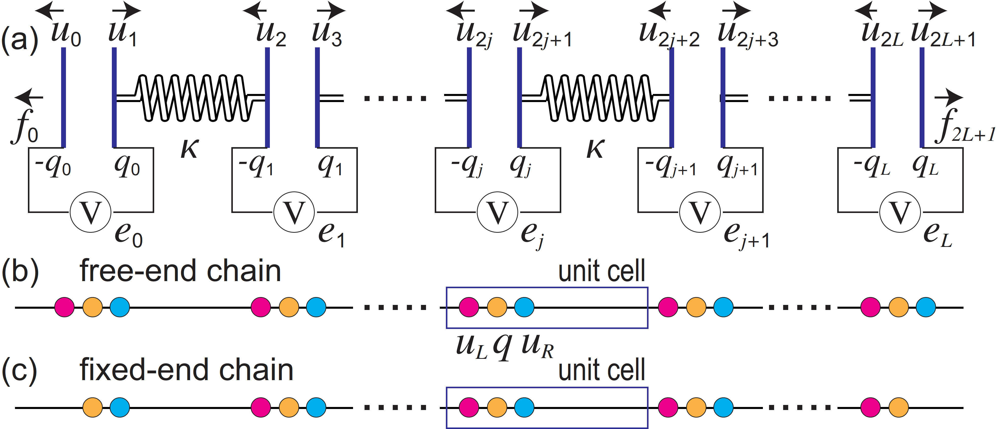
Figure 1: (a) Illustration of MEMS. Parallel metallic plates of capacitors can move, where adjacent plates are connected by insulating springs. The displacement $u_{j}$ of the $j$th plate is measured from its equilibrium position, while the charge $q_{j}$ is measured from the equilibrium charge $Q_{0}$ of the capacitor. Each capacitor is connected to a battery in order to charge up. One-dimensional tight-binding model (b) for a free-end chain and (c) for a fix-end chain, where the unit cell contains three sites marked in magenta, orange and cyan.

We explicitly write down the Euler-Lagrange equations (2) and (3), and expand them to the linear order in $u_{2j-1}$, $u_{2j}$ and $q_{j}$. Making the Fourier transformation from time $t$ to frequency $\omega$, we obtain for the $j$th unit cell (see Fig.1) that

$$f_{2j} =-M_{0}u_{2j}+\kappa u_{2j-1}+\frac{Q_{0}}{\varepsilon_{0}S}q_{j},$$ (4)

$$e_{j} =\frac{Q_{0}}{\varepsilon_{0}S}\left(u_{2j+1}+u_{2j}\right)+\frac{X_{\text{cap}}}{\varepsilon_{0}S}q_{j},$$ (5)

$$f_{2j+1} =-M_{0}u_{2j+1}+\kappa u_{2j+2}+\frac{Q_{0}}{\varepsilon_{0}S}q_{j},$$ (6)

where $M_{0}=m\omega^{2}-\kappa-\kappa_{0}-i\omega\gamma$.

We redefine the charge as $\hat{q}_{j}\equiv X_{\text{cap}}q_{j}/Q_{0}$ so that it has the dimension of length, and the voltage as $\hat{e}_{j}=Q_{0}e_{j}/X_{\text{cap}}$ so that it has the dimension of force. For a spatially periodic system, by making the Fourier transformation from the site index $j$ to momentum $k$ ($-\pi<k\leq\pi$), a set of equations (4), (5) and (6) is transformed into

$$\left(\begin{array}[]{c}f_{\text{L}}\\ \hat{e}\\ f_{\text{R}}\end{array}\right)=\left(\begin{array}[]{ccc}-M_{0}&Q&\kappa e^{-ik}\\ Q&Q&Q\\ \kappa e^{ik}&Q&-M_{0}\end{array}\right)\left(\begin{array}[]{c}u_{\text{L}}\\ \hat{q}\\ u_{\text{R}}\end{array}\right),$$ (7)

where $Q=Q_{0}^{2}/\left(X_{\text{cap}}\varepsilon_{0}S\right)$; $u_{\text{L}}(k)$, $\hat{q}\left(k\right)$ and $u_{\text{R}}(k)$ are the Fourier components of $u_{2j}$, $q_{j}$ and $u_{2j+1}$, while $f_{\text{L}}(k)$, $\hat{e}\left(k\right)$ and $f_{\text{R}}(k)$ are the Fourier components of $f_{2j}$ $\hat{e}_{j}$, and $f_{2j+1}$.

We represent Eq.(7) in the form of

$$\Phi_{fe}=J\Phi_{uq},$$ (8)

where $J$ is a $3\times 3$ matrix. We call $J$ the MEMS Laplacian as in the case of the circuit Laplacian in electric circuits, where $J$ has the dimension of spring constant.

A finite length chain may have either free ends or fixed ends. In the present problem, the free-end (fixed-end) oscillation occurs when a chain is terminated at the positions of the capacitor planes $u_{L}$ and $u_{R}$ (charge $q$) as in Fig.1(b) [(c)]. Note that the free-end chain respects the unit cell, but the fixed-end chain does not.

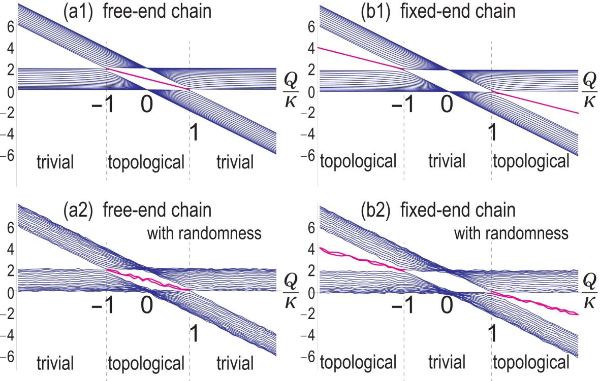
Figure 2: (a1) Eigen spectra of the part ($K-\kappa_{0}I_{2}$) of the dynamical matrix for a free-end chain and (b1) that for a fix-end chain in the case of free oscillation. The emergence of topological edge states marked in magenta differentiates the topological and the trivial phases. The horizontal axis is $Q/\kappa$. Only the region $Q/\kappa>0$ is physical. We have set $\gamma=0$. (a2) and (b2) are those with inclusion of randomness distributing uniformly from $-0.1\kappa$ to $0.1\kappa$ in the spring constants $\kappa$, $\kappa_{0}$ and the charge $Q_{0}$.

Free oscillation: First, we study the case of free oscillation in the absence of external force $f$ and voltage $e$, $\Phi_{fe}=0$, where Eq.(8) becomes $J\Phi_{xq}=0$. The charge is solved as $\hat{q}=-\left(u_{\text{L}}+u_{\text{R}}\right)$. We use it to eliminate $\hat{q}$ from Eq.(7), and obtain the kinetic equation,

$$m\frac{d^{2}}{dt^{2}}+\gamma\frac{d}{dt}\left(\begin{array}[]{c}u_{\text{L}}\\ u_{\text{R}}\end{array}\right)=-K\left(\begin{array}[]{c}u_{\text{L}}\\ u_{\text{R}}\end{array}\right),$$ (9)

with the dynamical matrix $K=(\kappa+\kappa_{0}-Q)I_{2}-H_{\text{SSH}}$, where $H_{\text{SSH}}$ is the SSH model,

$$H_{\text{SSH}}=\left(\begin{array}[]{cc}0&Q-\kappa e^{-ik}\\ Q\mathcal{-}\kappa e^{ik}&0\end{array}\right).$$ (10)

The spring constant $\kappa$ becomes $\kappa+\kappa_{0}-Q$ for $H_{\text{SSH}}=0$. This is known as the soft spring effect in the context of MEMS. We can tune $\kappa_{0}$ to make all the eigenvalues of $K$ positive.

The phase diagram is constructed as a function of the dimensionless parameter $Q/\kappa$. The SSH model is topological (trivial) for $|Q/\kappa|<1$ and trivial (topological) $|Q/\kappa|>1$, as is clear for a free-end (fixed-end) chain in Fig.2(a1) and (b1). The topological number is the winding number given by $W=\frac{1}{2\pi i}\int\left\langle\psi\right|\partial_{k}\left|\psi\right\rangle dk$, where $\psi$ is the eigenfunction of $H_{\text{SSH}}$. It is $1$ for the topological phase and $0$ for the trivial phase. It defines chiral-symmetry-protected topological (chiral-SPT) phases.

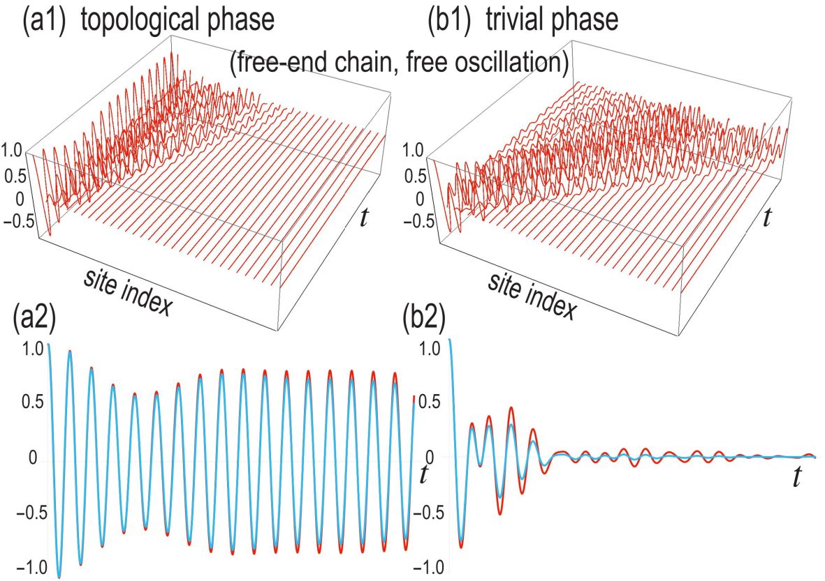
Figure 3: (a1) Time evolution of the plate displacement $u_{j}(t)$ in the topological phase with $Q/\kappa=0.5$ and (b1) that in the trivial phase with $Q/\kappa=1.5$ for a free-end chain in the case of free oscillation. (a2) The time evolution of the outer-most plate displacement $u_{0}(t)$ continues to oscillate with a finite amplitude in the topological phase, while (b2) it damps rapidly in the trivial phase. We have set $\kappa_{0}=4$. In (a2) and (b2), red curves are for no damping ($\gamma=0$), which are overwritten by cyan curves with damping ($\gamma=0.1\kappa/\omega_{0}$). Note that $\gamma\sim 0.01\kappa/\omega_{0}$ in actual samples, whose effects are negligible.

We show the time evolution of the plate displacement $u_{j}(t)$ in Fig.3(a1) and (b1) for all $j$. We impose the initial condition such that only the outermost plate at $j=0$ is displaced with the initial zero velocity. An oscillation propagates into the bulk in both the topological and the trivial phases. However, there is a significant difference. In the trivial phase the oscillation propagates rapidly into the whole bulk, but in the topological phase the oscillation is almost localized at the outermost plate. In particular, the outermost plate exhibits a salient oscillation dynamics. The outermost plate continues to oscillate with a finite amplitude in the topological phase, while it rapidly damps in the trivial phase. This is because its oscillation mode is almost isolated from (embedded in) the bulk spectrum in the topological (trivial) phase. We also show the time evolution of the plate in the presence of the damping term $\gamma$ in Fig.3(a2) and (b2). The oscillation damps but its effect is very small. Indeed, the damping is negligible since $\gamma\sim 10^{-2}\kappa/\omega_{0}$ in actual samples.

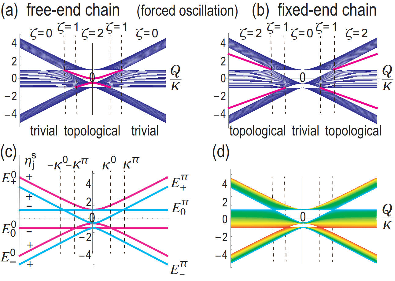
Figure 4: (a) Admittance spectrum for a finite free-end chain and (b) that for a finite fixed-end chain in the case of forced oscillation. We have set $M=1.5\kappa$. The horizontal axis is $Q/\kappa$, while the vertical axis is the admittance of the MEMS Laplacian. Topological edge states are marked in magenta. (c) Analytically obtained bulk admittance $E_{j}^{k}$ for $k=0$ and $\pi$. The signs $\eta_{j}^{k}=+$ and $-$ indicate the sign of the inversion-symmetry indicator. (d) Admittance spectrum for various $k$, where the color is ranging from $k=0$ marked in magenta to $k=\pi$ marked in cyan. Only the region $Q/\kappa>0$ is physical. We have set $\gamma=0$.

A comment is in order with respect to chiral symmetry. In actual samples, chiral symmetry is broken by randomness in the spring constants $\kappa$, $\kappa_{0}$ and the charge $Q_{0}$. Hence, strictly speaking, the system has no SPT phases. Nevertheless, even if we introduce fluctuations as much as 10% in these material constants, the topological edge states are found to be robust as shown in Fig.2(a2) and (b2), although the admittance of the edge states slightly shifts. Consequently, the topological dynamics of MEMS is experimentally observable in actual samples with randomness.

Forced oscillation: We next investigate a forced oscillation driven by external force or voltage periodic in time. We introduce a new quantity $H_{\text{tri}}$ by $H_{\text{tri}}=J+M_{0}I_{3}$,

$$H_{\text{tri}}=\left(\begin{array}[]{ccc}0&Q&\kappa e^{-ik}\\ Q&M-\kappa&Q\\ \kappa e^{ik}&Q&0\end{array}\right).$$ (11)

with $M=m\omega^{2}-\kappa_{0}+Q-i\omega\gamma$. Here, we have made explicit how $H_{\text{tri}}$ depends on $Q$ and $\kappa$. It is a key observation that $H_{\text{tri}}$ is identical to the Hamiltonian of a trimer modelAgar ; Jin ; Alva on one-dimensional lattice, where the unit cell contains three sites, as illustrated in Fig.1(b) and (c).

The trimer-model Hamiltonian has inversion symmetry $PH_{\text{tri}}\left(k\right)P^{-1}=H_{\text{tri}}\left(-k\right)$, where

$$P=\left(\begin{array}[]{ccc}0&0&1\\ 0&1&0\\ 1&0&0\end{array}\right).$$ (12)

It plays a key role to define inversion-SPT phases.

There are two inversion-symmetric momenta $k=0,\pi$. At these points, the eigenenergies $E_{j}^{k}$ and eigenfunctions $\psi_{j}^{k}$ are analytically obtained,

$$E_{0}^{0} =-\kappa,\quad E_{\pm}^{0}=\frac{M}{2}\pm\frac{\sqrt{\left(M-2\kappa\right)^{2}+8Q^{2}}}{2},$$ (13)

$$E_{0}^{\pi} =\kappa,\quad E_{\pm}^{\pi}=\frac{M}{2}-\kappa\pm\frac{\sqrt{M^{2}+8Q^{2}}}{2},$$ (14)

$$\psi_{0}^{k} =(-1,0,1)/\sqrt{2},\quad\psi_{\pm}^{k}=(1,F_{\pm}^{k},1)/\sqrt{2+F_{\pm}^{2}},$$ (15)

with

$$F_{\pm}^{0} =\{M-2\kappa\pm\sqrt{\left(M-2\kappa\right)^{2}+8Q^{2}}\}/\left(2Q\right),$$ (16)

$$F_{\pm}^{\pi} =\{M\pm\sqrt{M^{2}+8Q^{2}}\}/\left(2Q\right).$$ (17)

We show the spectrum $E_{j}^{k}(Q)$ in Fig.4(c), where the horizontal axis is a dimensionless quantity $Q/\kappa$. By solving $E_{\pm}^{0}(Q)=E_{0}^{0}(Q)$, we obtain a gap closing point $\pm Q^{0}$ with $Q^{0}=\sqrt{M\kappa}$. By solving $E_{\pm}^{\pi}(Q)=E_{0}^{\pi}(Q)$, we obtain two gap closing points $\pm Q^{\pi}$ with $Q^{\pi}=\sqrt{\kappa\left(2\kappa-M\right)}$. They are the endpoints of the magenta curves in Fig.4(a) and (b).

Topological edge states: The admittance is the eigenvalue of the MEMS Laplacian $J$. We show the admittance spectrum of a finite length chain as a function of $Q/\kappa$ in Fig.4(a) and (b). The magenta curves express edge states isolated from the bulk spectra at each $\kappa$. As suggested by the bulk-edge correspondence, they would be topological edge states at for $\left|Q\right|<Q^{0}$ for the lower band and $\left|Q\right|<Q^{\pi}$ for the upper band in Fig.4(a), and for $\left|Q\right|>Q^{0}$ for the lower band and $\left|Q\right|>Q^{\pi}$ for the upper band in Fig.4(b). To confirm this observation, we define the topological charge counting the number of magenta curves in what follows. Then, the phase diagram is given in term of a dimensionless parameter $Q/\kappa$ as in Fig.4(a) and (b).

Inversion-symmetry indicator: One dimensional system with inversion symmetry is classifiedInvClass ; Shiozaki into the class $\mathbb{Z}$. See Table VII class A with $\delta=1$ in Ref.Shiozaki . Symmetry indicators are good candidates to characterize SPT phasesWang ; Po ; Song ; Khalaf ; PoJ ; Slager . The inversion symmetry operator acts on the eigenfunctions as $P\psi_{0}^{k}=\eta_{0}^{k}\psi_{0}^{k}$, $P\psi_{\pm}^{k}\left(k\right)=\eta_{\pm}^{k}\psi_{\pm}^{k}\left(k\right)$, with $\eta_{0}^{k}=-1$ and $\eta_{\pm}^{k}=1$, where $k=0,\pi$. We define the inversion-symmetry indicator for the occupied band by $\zeta^{k}=\sum_{j}\eta_{j}^{k}$, where the sum over $j=0,\pm$ is taken for all occupied bands. See Fig.4(c), where $\eta_{j}^{k}=\pm$ is assigned to each curve $E_{j}^{k}(\kappa)$.

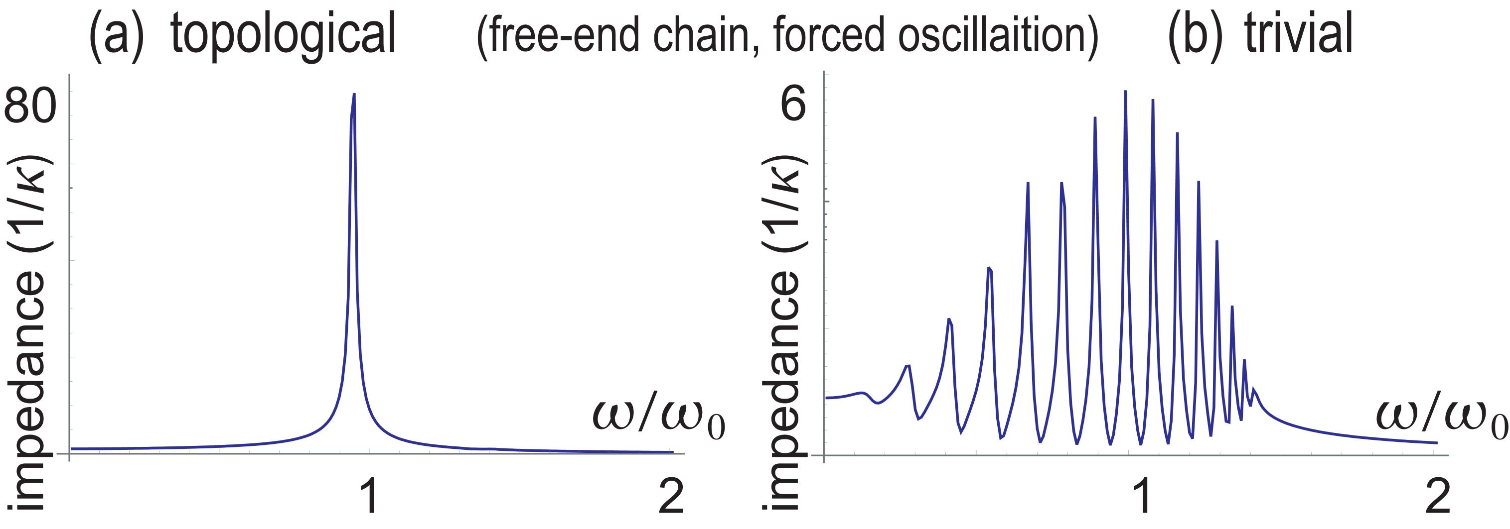
Figure 5: (a) Absolute value of electromechanical impedance in the topological phase with $Q=0.25$ and (b) that in the trivial phase with $Q=2$ in a free-end chain in the case of forced oscillation. It depends sensitively on the damping factor $\gamma$. Here, we have used a realistic value, $\gamma=0.01\kappa/\omega_{0}$. It diverges for $\gamma=0$. The horizontal axis is the driving frequency $\omega/\omega_{0}$ with $\omega_{0}=\sqrt{\kappa/m}$. We have set $Q-\kappa_{0}=0.5\kappa$. We have used a finite chain containing 48 sites.

We now define the topological number $\zeta$ with the use of the inversion-symmetry indicators so that $\zeta$ is nonzero for the topological phase and $\zeta=0$ for the trivial phase. (i) For a free-end chain, we define the number $\zeta_{\text{low}}=|\zeta^{\pi}-\zeta^{0}|/2$ for the lowest spectrum. We obtain $\zeta_{\text{low}}=1$ for $\left|Q\right|<Q^{0}$, while we obtain $\zeta_{\text{low}}=0$ for $\left|Q\right|>Q^{0}$, which counts the number of the lower edge states. In the similar way, the number of the upper edge states is counted by the number $\zeta_{\text{high}}=|\zeta^{\pi}-\zeta^{0}|/2$ for the highest spectrum, that is, $\zeta_{\text{high}}=1$ for $\left|Q\right|<Q^{\pi}$ and $\zeta_{\text{high}}=0$ for $\left|Q\right|>Q^{\pi}$. The topological number is given by $\zeta=\zeta_{\text{low}}+\zeta_{\text{high}}$, which agrees with the number of topological edge states shown in Fig.4. (ii) For a fixed-end chain, it is enough to define the topological number $\zeta$ in terms of $\zeta_{\text{low}}$ and $\zeta_{\text{high}}$ given by $|\zeta^{\pi}+\zeta^{0}|/2$.

Electromechanical impedance: Impedance resonance is a good signal to detect topological edge states in electric circuitsTECNature ; ComPhys ; EzawaTEC . We now show that the electromechanical impedance well signals the emergence of the topological edge states. We define the electromechanical impedance by the inverse of the MEMS Laplacian, i.e., by $Z=J^{-1}=G$, where $G$ is the Green function. It is obtained by measuring the displacement $u$ and the charge $q$ induced under the application of the force $f$ or voltage $e$ by way of the relation (8) or $\Phi_{uq}=Z\Phi_{fe}$.

For a semi-infinite free-end chain, the left-upper most component of the Green function is $G_{00}$, which is expressed in terms of a continued fraction $G_{00}=\mathcal{G}/\kappa^{2}$ as

$$\mathcal{G}=\frac{1}{-M_{0}-\frac{Q^{2}}{Q-\frac{Q^{2}}{-M_{0}-\frac{\kappa^{2}}{-M_{0}-\cdots}}}}=\frac{1}{-M_{0}-\frac{Q^{2}}{Q-\frac{Q^{2}}{-M_{0}-\kappa^{2}\mathcal{G}}}}.$$ (18)

It is solved in a closed form as

$$\mathcal{G}=[\left(\kappa^{2}+M_{0}^{2}\right)+2M_{0}Q\pm\sqrt{\mathcal{M}}]/[2\left(Q+M_{0}\right)],$$ (19)

with $\mathcal{M}=Q\left(M_{0}^{2}-\kappa^{2}\right)\left[\left(2Q+M_{0}\right)^{2}-\kappa^{2}\right]$. The impedance diverges at $\omega=\sqrt{(\kappa-Q)/m}$. We show the impedance $Z_{00}$ for a finite free-end chain as a function of $\omega$ in Fig.5. It measures the response of the plate displacement $u_{0}$ when we apply a force $f_{0}$ with frequency $\omega$.

There is a single strong impedance resonance peak in the topological phase as shown in Fig.5(a). It reflects the fact that the left most plate $u_{1}$ is almost isolated in the topological phase. On the other hand, there are many small peaks in the trivial phase as shown in Fig.5(b). This is because the oscillation propagates to other plates. The number of peaks increases as the length increases.

In passing, we provide typical values of sample parametersMita1 ; Mita2 . They are $C=10$pF, $m=100\mu$g, $X_{\text{cap}}=100\mu$m, $\kappa=10$N$/$m, which lead to the resonant frequency around $\omega_{0}=10$kHz. A typical value of the damping factor is $\gamma=10^{-5}$kg$/$s. As far as we are aware, there is no literature on the topological MEMS. It will be possible to construct such a MEMS with current technologyMitaP .

In this work we have revealed a novel topological dynamics of MEMS. We have argued that it is experimentally observable in actual samples with randomness and damping. Our results will open an attractive field of topological MEMS.

The author is very much grateful to Y. Mita, M. Sato and N. Nagaosa for helpful discussions on the subject. This work is supported by the Grants-in-Aid for Scientific Research from MEXT KAKENHI (Grants No. JP17K05490 and No. JP18H03676). This work is also supported by CREST, JST (JPMJCR16F1 and JPMJCR20T2).

References

- (1) X.-L. Qi, S.-C. Zhang, Rev. Mod. Phys. 83, 1057 (2011).
- (2) L. Lu, J. D. Joannopoulos and M. Soljacic, Nat. Phtonics 8, 821 (2014).
- (3) T. Ozawa, H. M. Price, A. Amo, N. Goldman, M. Hafezi, L. Lu, M. C. Rechtsman, D. Schuster, J. Simon, O. Zilberberg and I. Carusotto, Rev. Mod. Phys. 91, 015006 (2019).
- (4) A. B. Khanikaev, S. H. Mousavi, W.-K. Tse, M. Kargarian, A. H. MacDonald and G. Shvets, Nat. Mat. 12, 233 (2013).
- (5) M. Xiao, G. Ma, Z. Yang, P. Sheng, Z. Q. Zhang and C. T. Chan, Nat. Phys. 11, 240 (2015).
- (6) Z. Yang, F. Gao, X. Shi, X. Lin, Z. Gao, Y. Chong, and B. Zhang, Phys. Rev. Lett. 114, 114301 (2015).
- (7) S. H. Mousavi, A. B. Khanikaev and Z. Wang, Nat. Com. 6, 8682 (2015).
- (8) M. Serra-Garcia, V. Peri, R. Susstrunk, O. R. Bilal, T. Larsen, L. G. Villanueva, and S. D. Huber, Nature 555, 342 (2018).
- (9) H. Xue, Y. Yang, F. Gao, Y. Chong and B.Zhang, Nature Materials 18, 108 (2019).
- (10) X. Ni, M. Weiner, A. Alu and A. B. Khanikaev, Nature Materials 18, 113 (2019).
- (11) E. Prodan and C. Prodan, Phys. Rev. Lett. 103, 248101 (2009).
- (12) C. L. Kane and T. C. Lubensky, Nature Phys. 10, 39 (2014).
- (13) L. M. Nash, D. Kleckner, A. Read, V. Vitelli, A. M. Turner and W. T. M. Irvine, PNAS 112, 14495 (2015).
- (14) R. Susstrunk, S. D. Huber, Science 349, 47 (2015).
- (15) T. Kariyado and Y. Hatsugai, Sci. Rep. 5, 18107 (2016).
- (16) Y. Takahashi, T. Kariyado and Y. Hatsugai, New J. Phys. 19, 035003 (2017).
- (17) A. S. Meeussen, J. Paulose and V. Vitelli, Phys. Rev. X 6, 041029 (2016).
- (18) H. Abbaszadeh, A. Souslov, J. Paulose, H. Schomerus and V. Vitelli, Phys. Rev. Lett. 119, 195502 (2017).
- (19) K. H. Matlack, M. Serra-Garcia, A. Palermo, S. D. Huber and C. Daraio, Nature Mat. 17, 323 (2018).
- (20) S. Imhof, C. Berger, F. Bayer, J. Brehm, L. Molenkamp, T. Kiessling, F. Schindler, C. H. Lee, M. Greiter, T. Neupert, R. Thomale, Nat. Phys. 14, 925 (2018).
- (21) C. H. Lee , S. Imhof, C. Berger, F. Bayer, J. Brehm, L. W. Molenkamp, T. Kiessling and R. Thomale, Communications Physics, 1, 39 (2018).
- (22) T. Helbig, T. Hofmann, C. H. Lee, R. Thomale, S. Imhof, L. W. Molenkamp and T. Kiessling, Phys. Rev. B 99, 161114 (2019).
- (23) K. Luo, R. Yu and H. Weng, Research (2018), ID 6793752.
- (24) E. Zhao, Ann. Phys. 399, 289 (2018).
- (25) M. Ezawa, Phys. Rev. B 98, 201402(R) (2018).
- (26) M. Serra-Garcia, R. Susstrunk and S. D. Huber, Phys. Rev. B 99, 020304 (2019).
- (27) T. Hofmann, T. Helbig, C. H. Lee, M. Greiter, R. Thomale, Phys. Rev. Lett. 122, 247702 (2019).
- (28) M. Ezawa, Phys. Rev. B 99, 201411 (2019).
- (29) M. Ezawa, Phys. Rev. B 99, 121411 (2019).
- (30) M. Ezawa, Phys. Rev. B 100, 045407 (2019).
- (31) M. Ezawa, Phys. Rev. B 102, 075424 (2020).
- (32) X. Liu and G.S. Agarwal, Scientific Reports 7, 45015 (2017).
- (33) L Jin, Physical Review A 96, 032103 (2017).
- (34) V. M. Martinez Alvarez, M. D. Coutinho-Filho, Phys. Rev. A 99, 013833 (2019).
- (35) Y. M. Lu and D. H. Lee, arXiv:1403.5558
- (36) K. Shiozaki and M. Sato, Phys. Rev. B 90, 165114 (2014).
- (37) Z. Wang, B. J. Wieder, J. Li, B. Yan, B. A. Bernevig, Phys. Rev. Lett. 123, 186401 (2019).
- (38) H. C. Po, A. Vishwanath and H. Watanabe, Nat. Comm. 8, 50 (2017).
- (39) Z, Song, T. Zhang, Z. Fang and C. Fang, Nat. Com. 9, 3530 (2018).
- (40) E. Khalaf, H. C. Po, A. Vishwanath and H. Watanabe, Phys. Rev. X 8, 031070 (2018).
- (41) H. C. Po, J. Phys.: Condens. Matter 32, 263001 (2020).
- (42) J. Kruthoff, J. de Boer, J. van Wezel, C. L. Kane, and R.-Jan Slager Phys. Rev. X 7, 041069 (2017).
- (43) Y. Mita, A. Hirakawa, B. Stefanelli, I. Mori, Y. Okamoto, S. Morishita, M. Kubota, E. Lebrasseur, A. Kaiser, Japanese Journal of Applied Physics, 57 04FA05 (2018)
- (44) R. Reddy, K. Komeda, Y. Okamoto, E. Lebrasseur, A. Higo, Y. Mita, Sensors and Actuators A: Physical, 295, 1 (2019)
- (45) Y. Mita, private communications.