Dense U-net for single image super-resolution with shuffle pooling layer

Abstract

Recent researches have achieved great progress on single image super-resolution(SISR) due to the development of deep learning in the field of computer vision. In these method, the high resolution input image is down-scaled to low resolution space using a single filter, commonly max-pooling, before feature extraction. This means that the feature extraction is performed in biased filtered feature space. We demonstrate that this is sub-optimal and causes information loss. In this work, we proposed a state-of-the-art convolutional neural network method called Dense U-net with shuffle pooling. To achieve this, a modified U-net with dense blocks, called dense U-net, is proposed for SISR. Then, a new pooling strategy called shuffle pooling is designed, which is aimed to replace the dense U-Net for down-scale operation. By doing so, we effectively replace the handcrafted filter in the SISR pipeline with more lossy down-sampling filters specifically trained for each feature map, whilst also reducing the information loss of the overall SISR operation. In addition, a mix loss function, which combined with Mean Square Error(MSE), Structural Similarity Index(SSIM) and Mean Gradient Error (MGE), comes up to reduce the perception loss and high-level information loss. Our proposed method achieves superior accuracy over previous state-of-the-art on the three benchmark datasets: SET14, BSD300, ICDAR2003. Code is available online.

1 Introduction

Single image super-resolution can be used as an effective data argumentation method for most image processing tasks, such as object detection, object recognition, target tracking and instance segmentation. However, various image types under different complex environments impose great challenges for super-resolution in real-world applications.

The global SR problem assumes high-resolution feature map has glut redundant information which treated as noisy and culled in down-sampling operation. It is a highly necessary to be concerned with this information loss problem due to directly remove pixels in down-sampling such as max-pooling and average-pooling.

Many methods assume that the deeper convolutional network have better ability to extract semantic and perceptual features. However, not only the first proposed super-resolution method Super-Resolution Convolution Neural Network (SRCNN) dong2015image , but also the following representative methods, which includes Very Deep network for Super-Resolution (VDSR) kim2016accurate , Deeply-Recursive Convolutional Networks (DRCN) kim2016deeply and Deep Back-Projection Networks (DBPN) haris2018deep , is committed to designing deeper networks to obtain more perceptual features with a single-channel feature extraction and single-channel up-sampling module. By doing so, these methods largely ignored the loss of low-level texture information since the single-channel overemphasizes high-level semantic information.

In short, previous works inherently limited to defects in the information transmission structure. Take U-net as an example, first, the skip-connections between the same depth convolution layers are only one-way. Second, traditional max-pooling method caused more than ($\frac{2^{k}-1}{2^{k}}$) of information loss in each down-sampling block when down-scale is $k$ due to directly drop ($2^{k}-1$) pixel values. Third, previous methods focus on evaluation method of Peak Signal to Noise Ratio (PSNR), which result in the high performance on PSNR, but largely ignored the gradient error. In general, previous methods lacked lossless mechanisms to handle information transfer processing. To solve these problems, we propose the Dense UnetSR, which combines the Dense U-net for super-resolution with shuffle pooling method, that greatly enhances the capability of the information transfer mechanism.

To solve these problems, this paper has the following four contributions:

1. we propose a state-of-the-art convolutional neural network method called Dense U-net with shuffle pooling. Compare with U-net ronneberger2015u for SISR, Dense U-net enhances the skip-connection part by transmitting all feature layers from different depth to each up-sampling layer. It reduces the information transmission loss because the up-sampling block combines all down-sampling feature maps from all depth of contracting blocks.

2. A novel pooling method called shuffle pooling is designed for the Dense U-net, which can effectively replace the handcrafted filter in the SISR pipeline with more lossy down-sampling filters specifically trained for each feature map, whilst also reducing the information loss of the overall SISR operation. As shown in Fig. 3, shuffle pooling module consists of 2 steps: 1) Sampling the input feature map by specified intervals; 2) Reshaping sampled values into down-sampled feature maps.

3. The mix loss function, which combined with Mean Square Error(MSE) huynh2008scope , Structural Similarity Index (SSIM) hore2010image and Mean Gradient Error(MGE) lu2019single , basically solves the perception loss and high-frequency information loss. Besides MSE loss, the MixE loss considers SSIM loss which helps to better restore brightness, contrast and structure, and MGE loss which helps to better restore sharpness of images.

4. The proposed Dense UnetSR outperforms the state-of-the-art the SISR methods in SET14, BSD300, ICDAR2003 datasets, especially in the text tasks.

2 Related work

He et al. dong2015image introduced the first deep learning method for single image super-resolution (SISR) task called Super-Resolution Convolution Neural Network (SRCNN). SRCNN simply constructs a multi-layer convolutional network directly without considering transmission loss and computational complexity.

In order to reduce the computational complexity of the SRCNN, Fast Super-Resolution Convolutional Neural Network (FSRCNN) dong2016accelerating built a lightweight framework to solve the real-time problem. FSRCNN Instead of taking interpolated image by Bicubicde1962bicubic as input, FSRCNN directly put the LR image into the network, and up-scaled by deconvolution layer finally. Although FSRCNN has reduced the running time of the SRCNN by more than 70%, its low accuracy made it difficult to be applied in real scenes.

Efficient Sub-Pixel Convolutional Neural (ESPCN) shi2016real introduced an efficient sub-pixel convolution layer which learns an array of up-scaling filters to upscale the low-resolution image into the high-resolution output. Inspired by ResNet he2016deep , Very Deep network for Super-Resolution (VDSR) kim2016accurate was proposed to solve the training problem of deeper super-resolution networks.

VDSR built an end-to-end network with 20 convolution layers by cascading small filters many times in a deep network structure. Super-Resolution Generative Adversarial Networks (SRGAN) ledig2017photo were the first Generative Adversarial Networks (GAN) goodfellow2014generative for super-resolution task the first to consider the human subjective evaluation of reconstructed images. In order to improve the accuracy and perceptual evaluation, SRGAN was extremely hard to converge during the training process.

Enhanced Deep Residual Networks for Super-Resolution (EDSR) lim2017enhanced achieved the highest score in the NTIRE2017 Super-Resolution Challenge Competition Agustsson2017NTIRE . The most significant performance improvement of EDSR was to remove the redundant modules of SRResNet which is the generator network of SRGAN ledig2017photo , so that the size of the model can be enlarged to improve the image quality.

Deeply-Recursive Convolutional Networks (DRCN) kim2016deeply and Deep Back-Projection Networks (DBPN) haris2018deep exploited iterative up-sampling and down-sampling and DBPN had better performance because it provided an error feedback mechanism. Although DRCN and DBPN reduced the number of parameters, these methods did not actually solve the problem of high computational complexity due to too much repetitive calculations.

Image Super-Resolution Using Very Deep Residual Channel Attention Networks(RCAN)zhang2018image reached much deeper by residual in residual structure than other CNN-based methods and obtained a better performance. The long and short skip connections in residual in residual structure helped to bypass abundant low-frequency information and made the main network learn more effective information. Then, channel attention mechanism is proposed to adaptively rescale features by considering interdependencies among feature channels.

To solve the problem of Hindering the representational power of CNNs caused by neglecting to explore the feature correlations of intermediate layers, the second-order attention network(SAN)dai2019second was proposed for for more powerful feature expression and feature correlation learning. Specifically, the novel trainable second-order channel attention module was developed to adaptively rescale the channel-wise features by using second-order feature statistics for more discriminative representations. Furthermore, Daidai2019second presented a non-locally enhanced residual group structure, which not only incorporates non-local operations to capture long-distance spatial contextual information, but also contains repeated local-source residual attention groups to learn increasingly abstract feature representations.

The U-net for Super-Resolution (UnetSR) lu2019single modified the basic U-net architecture to adapt to the field of SISR and proposed a mix gradient loss function to enhance the sharpness of reconstructed images. Although the problem of image blur is considered, UnetSR still has many defects in network transmission.

3 Approach

In this section, the architecture of Dense U-net for super-resolution with shuffle pooling layer will be described as three parts: 1) Dense U-net network; 2) Shuffle pooling method; 3) Mix loss function.

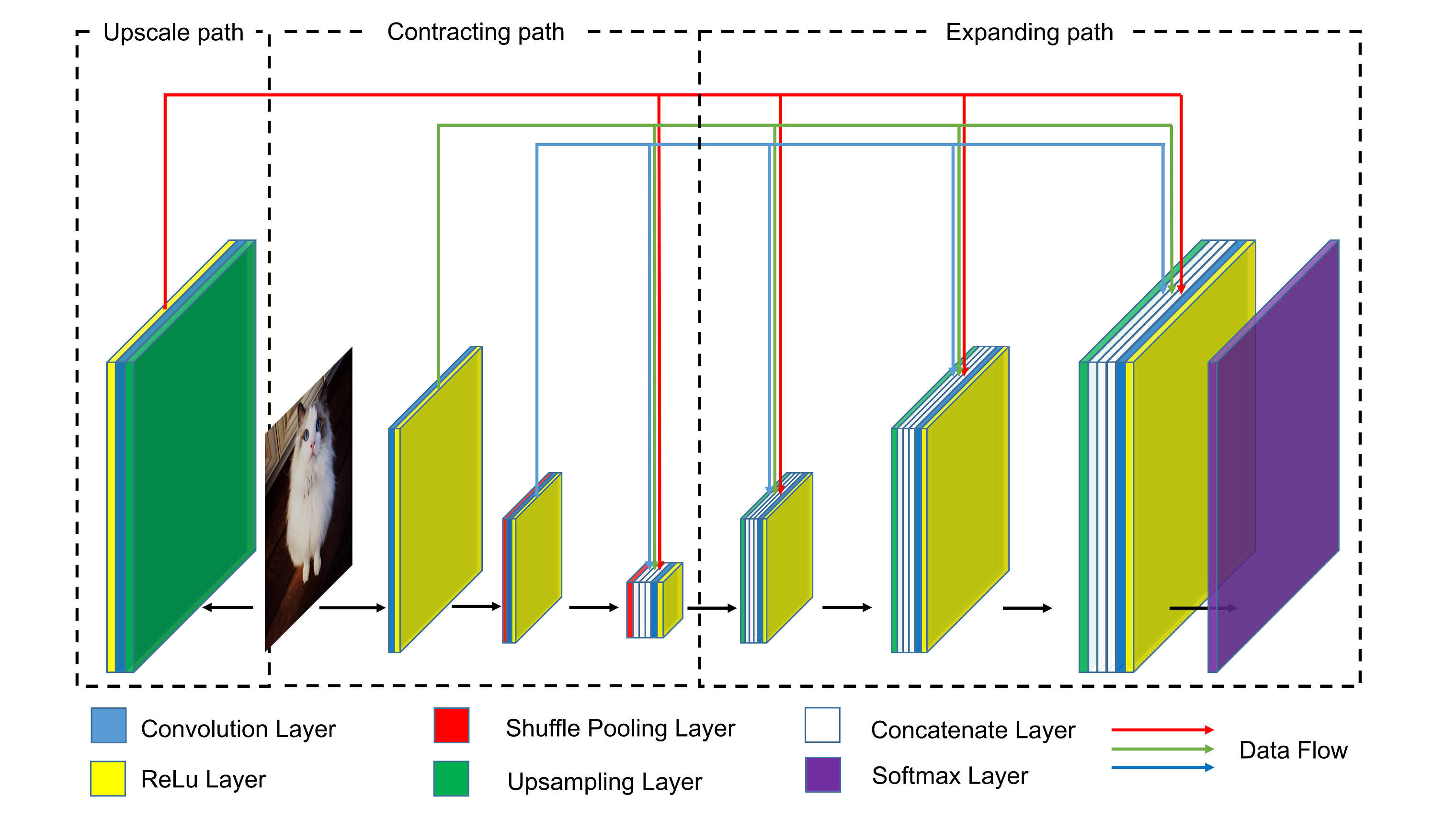
Figure 1: Architecture of Dense U-net for super-resolution task, where the depth of the network is 3 and the up-scale is 2.

3.1 Overall Framework

The overall pipeline of our approach is shown in Fig. 1. the network consists of three main parts: upscale path for the pre-upsampling, contracting path for the feature extraction and expanding path for the image reconstruction. The proposed Dense U-net is taken as the backbone of the network. The novel shuffle pooling strategy is designed to replace traditional pooling methods.

3.2 Dense U-net

The Dense UnetSR for super-resolution is an improved UnetSR lu2019single by combining dense blocks into the network. As illustrated in Fig. 1, the network consists of four parts:

3.2.1 Contracting path

The left side of Dense UnetSR is the contracting path for extracting features. The contracting path contains the continues part of one $3\times 3$ kernel, followed by a Rectified Linear Unit (ReLU) layer, and then a $2\times 2$ max-pooling operation with stride 2 for down-sampling. The U-Net ronneberger2015u is modified for SISR task by removing all batch normalization layers and one convolution layer in each block. To improve the down-sampling method, shuffle pooling method is applied into Dense UnetSR to replace the max-pooling method.

3.2.2 Expanding path

The right side of Fig. 1 is expanding path for decoding. Each block in the expansive includes an up-sampling of the feature map, which followed by a $2\times 2$ kernel that halves the number of feature maps, and one $3\times 3$ convolution kernel, followed by a ReLU layer.

3.2.3 Upscale path

The upscale path includes an up-sampling layer and a convolutional layer and meant to keep the same depth of contracting path and expanding path. The input image is up-sampling by bicubic interpolation and builds the symmetric feature extraction layer corresponds to the same depth up-sampling layer in expanding path.

3.2.4 Dense skip connection

The dense data skip-connections are constructed for transferring feature maps from all depth of contracting blocks into every expanding block. Because the up-sampling block combines all down-sampling feature maps from all depth of contracting blocks instead of feature maps from the one-way down-sampling path, theoretically the dense skip connection establishes a multi-path data transmission and reduces the information transmission loss.

3.3 Shuffle pooling

In most network architectures, general pooling methods including max-pooling and average-pooling were widely applied for down-sampling. In this work, a new pooling strategy called shuffle pooling is presented. As illustrated in Fig. 2, this module consists of 2 steps: 1) Sampling the input feature map by a specified interval; 2) Reshaping sampled values into down-sampled feature maps. According to the different arrangement of pooling layer, the shuffle pooling have two different strategies, namely directive and insertive shuffle pooling, which are shown in Fig. 3. Different from the max-pooling and average-pooling which keep one-quarter sampling, the proposed shuffle pooling maintains all information in the feature map of the previous layer. Meanwhile, shuffle pooling brings four times the channel number and four times the parameter amount.

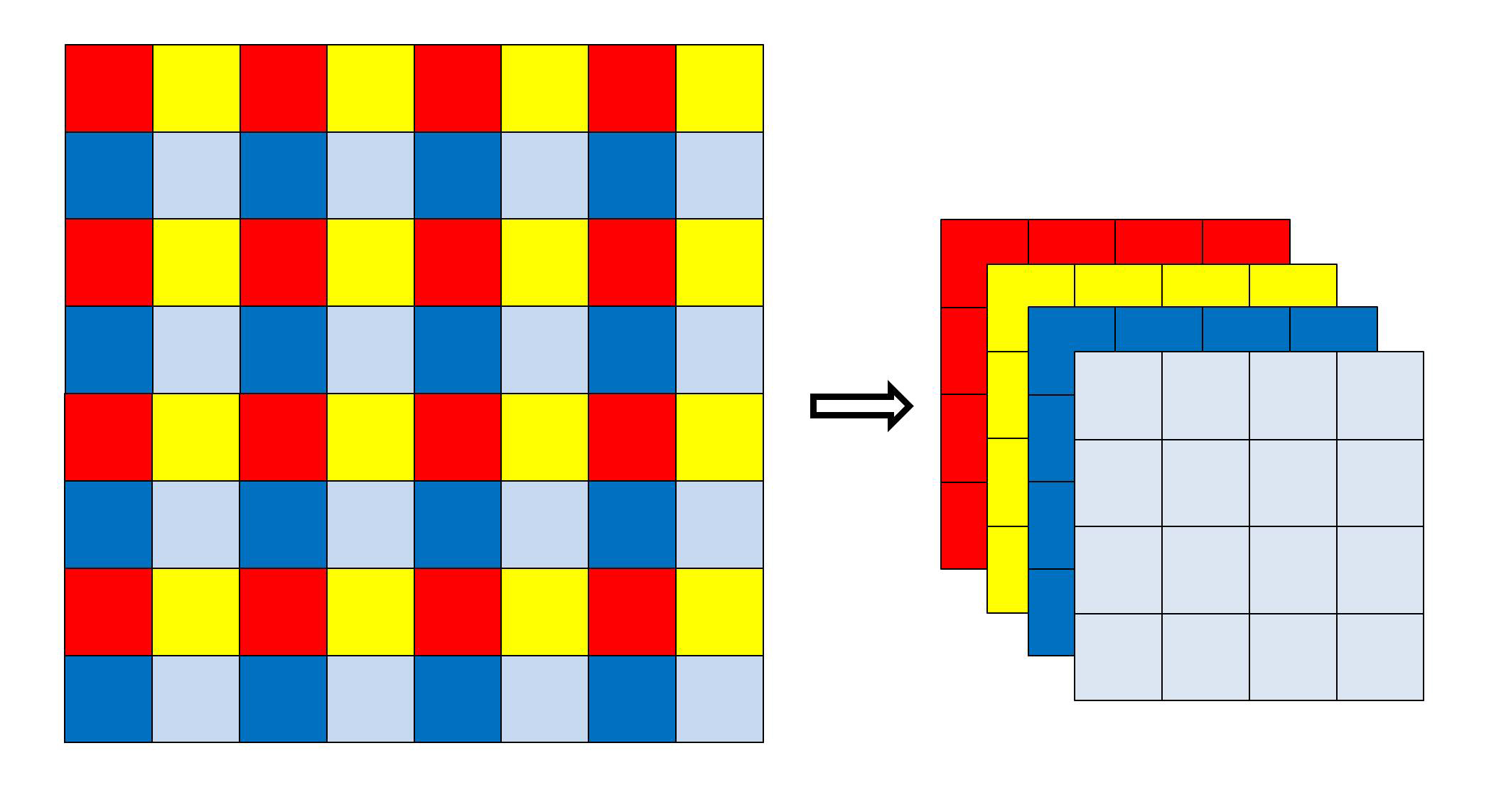
Figure 2: Shuffle pooling flow diagram, where the
down-scale is 2.

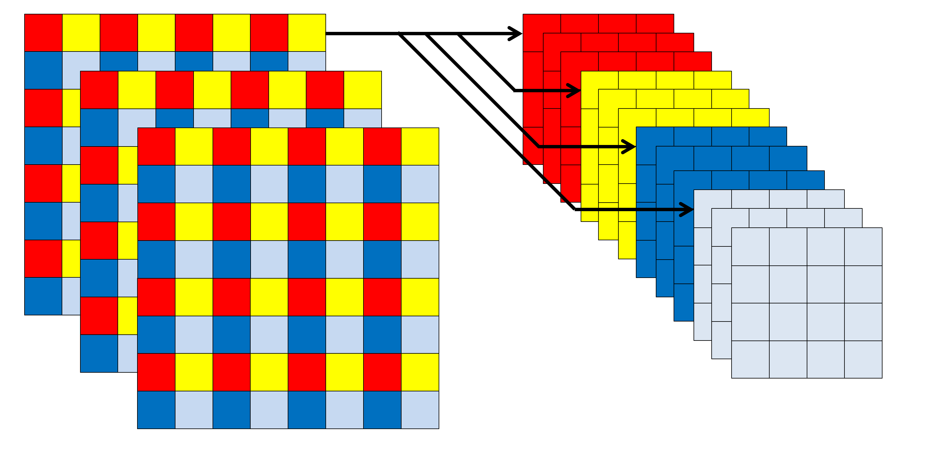
(a) Direct method

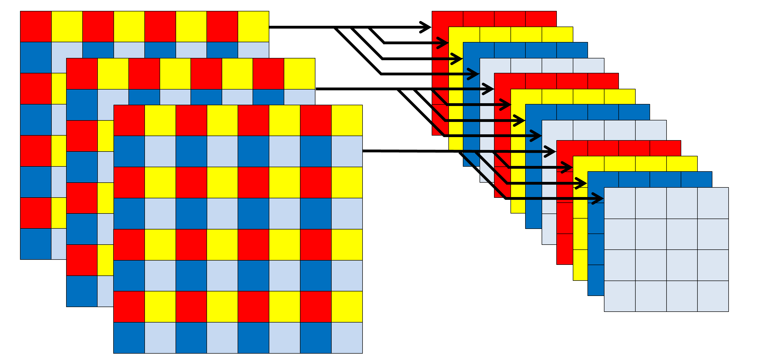
(b) Insert method

Figure 3: Different arrangements of pooling methods, where the down-scale is 2.

3.4 Mix loss function

In this subsection, we first analysize the problem of existing SISR which were only trained with Mean Square Error (MSE) loss. Then the three losses used for the proposed mix loss function, namely MSE loss, Structural Similarity Index (SSIM) loss and Mean Gradient Error (MGE) loss are introduced respectively. The mix loss function is presented at the end of the subsection.

3.4.1 Problem analysis

As shown in Fig. 4, most previous works on SISR task only trained by MSE loss function, therefore these methods had some shortcomings.

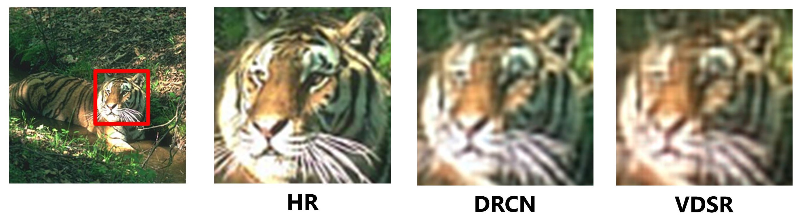
Figure 4: Super-resolution results by previous works with MSE loss($\times$ 4).

First, previous studies of SISR trained only by MSE loss had not dealt with the problem of blurred edge, shown as reconstructed results by DRCN and VDSR in Fig. 4. To preserve the sharpness of the reconstructed edges, it is necessary to take image gradient as one of the SISR constraints.

Second, MSE only focused on the error between each pixel and ground truth, which ignores the neighboring structure of pixels. SSIM gave us a new method to measure the structural similarity between reconstructed images and the ground truth, which can be applied in SISR task as a neighboring structure constraint to improve the structural similarity.

3.4.2 MSE loss

MSE reflects the variance between the current image and the source image at each pixel. Two criteria are described as follows. Let Y donates the ground truth and $\hat{Y}$ donates the reconstructed high-resolution images respectively.

$$\begin{split}MSE=\frac{1}{MN}\sum_{i=1}^{M}\sum_{j=1}^{N}(\hat{Y}(i,j)-Y(i,j))^{2}\end{split}$$ (1)

3.4.3 SSIM loss

The criterion of SSIM between patches $P_{\hat{Y}}$ and $P_{Y}$ at the same location on ground truth images $\hat{Y}$ and reconstructed high-resolution image $Y$ is defined as

$$\begin{split}SSIM(P_{\hat{Y}},P_{Y})=\frac{(2\mu_{P_{\hat{Y}}}\mu_{P_{Y}}+c_{1})(2\sigma_{P_{\hat{Y}}}\sigma_{P_{Y}}+c_{2})}{(\mu_{P_{\hat{Y}}}^{2}+\mu_{P_{Y}}^{2}+c_{1})(\sigma_{P_{\hat{Y}}}^{2}+\sigma_{P_{Y}}^{2}+c_{2})}\end{split}$$ (2)

where $\mu_{P_{\hat{Y}}}$ and $\mu_{P_{Y}}$ are the mean of patch $P_{\hat{Y}}$ and $P_{Y}$ respectively. Meanwhile, $\sigma_{P_{\hat{Y}}}$ and $\sigma_{P_{Y}}$ are the deviation of patch $P_{\hat{Y}}$ and $P_{Y}$. $c_{1}$ and $c_{2}$ are small constants. Then, The criterion of $SSIM(\hat{Y},Y)$ is the average of patch-based SSIM over the image.

3.4.4 MGE loss

To solve the gradient error measurement problem, we introduce classic gradients to the SISR loss function called Sobel operatorkanopoulos1988design . The gradient map $G$ in $x$ and $y$ direction of the ground truth image $Y$ shows below:

$$G_{x}=Y*\begin{bmatrix}-1&-2&-1\\ 0&0&0\\ 1&2&1\end{bmatrix}$$ (3)

$$G_{y}=Y*\begin{bmatrix}-1&0&1\\ -2&0&2\\ -1&0&1\end{bmatrix}$$ (4)

where $*$ is the convolution operation.

Then we combine the gradient value of $x$ and $y$ direction as follows:

$$G(i,j)=\sqrt{G_{x}^{2}(i,j)+G_{y}^{2}(i,j)}$$ (5)

Let G donates the ground truth and $\hat{G}$ donates the reconstructed high-resolution results. The aim of measure the gradient error is to learn a sharp edge which is close to the ground truth edge. The Mean Gradient Error (MGE) shows as follows:

$$\begin{split}MGE=\frac{1}{n}\frac{1}{m}\sum_{i=1}^{n}\sum_{j=1}^{m}(\hat{G}(i,j)-G(i,j))^{2}\end{split}$$ (6)

3.4.5 Mix loss function

After achieving the MGE, it should be emphasized in the mix gradient error. As the main component of mix gradient error, Mean Square Error forms a Mix Error (MixE) by adding Mean Gradient Error with a weight of $\lambda_{G}$ and SSIM with a weight of $\lambda_{S}$.

$$\begin{split}MixE(Y,\hat{Y})=MSE+\lambda_{G}MGE+\lambda_{S}SSIM\end{split}$$ (7)

Previous researches on SISR has tended to focus on network architecture rather than loss function. Therefore, the modified form of the loss function is applied to this experiment. To illustrate the superiority of mix loss function, a much more systematic inference would try to identify how network performance interacts with MixE that is believed to be linked to the fusion method.

4 Experiment

4.1 Dataset

ICDAR2003 karatzas2013icdar is a dataset of the ICDAR Robust Reading Competition for text detection and recognition tasks. Though the ICDAR2003 dataset is not commonly used for SISR task, it reflects the performance of these methods on text images. The ICDAR2003 dataset consists of 258 training images and 249 testing images, which contains texts in most of the common life complex circumstances. Because of the resolution of images varies from 422$\times$102 to 640$\times$480, we resize them into 224$\times$224 with bicubic interpolation. This network is also compared with other existing methods over standard benchmark datasets: SET14 bevilacqua2012low , BSD300 martin2001database .

4.2 Evaluation method

Two widely used evaluation methods, Peak Signal to Noise Ratio (PSNR) huynh2008scope and Structural Similarity Index (SSIM) hore2010image , are applied for comparison on image quality and similarity.

PNSR, which derived from MSE, reflects the ratio of peak signal to noise. The criteria of PSNR and SSIM are all based on luminance. The higher the value of these criteria, the better the performance of image reconstruction. Compared with MSE, the value of PSNR is positively correlated with image quality, which is more conducive to intuitive comparison.

$$\begin{split}PSNR(Y,\hat{Y})=10log_{10}\frac{255^{2}}{MSE}\end{split}$$ (8)

4.3 Implement details

Three datasets, SET14 bevilacqua2012low , BSD300 martin2001database and ICDAR2003 karatzas2013icdar , are chosen to evaluate these existed SISR methods. SET14 and BSD300 dataset consist of natural scenes and ICDAR2003 contain various types of texts in a robust common scene. In order to generate low-resolution and high-resolution image pairs for training and testing, the source images are down-scaled by bicubic interpolation on Table 1. Meanwhile, all images are converted into RGB colour space.

Table 1: Image size of different scales

Scale	Image size
	LR	HR
$\times$2	112$\times$112	224$\times$224
$\times$4	56$\times$56	224$\times$224
$\times$8	28$\times$28	224$\times$224

The MSE, which widely used in image reconstruction tasks, is chosen to be the loss function in this experiment. Two widely used evaluation methods, PSNR huynh2008scope and Structural Similarity Index (SSIM) hore2010image , are applied for comparison on image quality and similarity in our experiment.

In the training parameter set, the batch of data is set to $1$. Our method is trained by Adam optimizer kingma2014adam with $\beta_{1}=0.9$, $\beta_{2}=0.999$, $\epsilon=10^{-8}$. The learning rate is set to $10^{-3}$ initially and decreases to half every $50$ epochs. The PyTorch implement of our method is trained with one RTX 2080 GPU and this project is proposed online.

4.4 Network analysis

4.4.1 Dense U-net

To evaluate U-net and Dense U-net architecture, we train these methods on U-net and Dense U-net backbone with 5-layer depth over SET14, BSD300 and ICDAR2003 datasets. Data from the Table. 2 shows that the backbone of Dense U-net performs much better than the U-net on all three datasets. Because the insert method of shuffle pooling is better than the direct method from the Table. 2, the insert method is applied into all the following shuffle pooling method. U-net for super-resolution is simplified as UnetSR and Dense U-net for super-resolution without shuffle pooling is DensetSR. Meanwhile, Dense U-net with shuffle pooling layer is simplified as DensetSR+.

Table 2: Comparison of different shuffle pooling arrangements

Scale=2
Method	SET14	BSD300	ICDAR2003
	PSNR/SSIM	PSNR/SSIM	PSNR/SSIM
UnetSRa	26.7241/0.8889	29.4241/0.8832	35.8147/0.9307
UnetSR(Directb)	27.1581/0.8984	29.5013/0.8854	35.8964/0.9312
UnetSR(Insertc)	27.3221/0.9014	29.7188/0.8902	36.4241/0.9392
DenseSR	27.4011/0.9027	29.4902/0.8851	35.9829/0.9325
DenseSR(Direct)	27.4278/0.9033	29.5133/0.8858	35.9844/0.9327
DenseSR(Insert)	28.3938/0.9236	29.8478/0.8965	36.9244/0.9409
aThe max-pooling method is default to UnetSR and DenseSR.
bThis is the direct method of shuffle pooling.
cThis is the insert method of shuffle pooling.

4.4.2 Shuffle pooling

As Table. 2 shown, there is a significant improvement by replacing the max-pooling method with shuffle pooling. A comparison of the two arrangement methods in Table. 2 reveals the insert method of shuffle pooling achieves the higher PSNR than the direct method, with +0.94 dB on SET14 dataset, +0.97 dB on BSD300 dataset and +1.10 dB on ICDAR2003 dataset.

4.4.3 Mix loss function

In order to determine the best value of the weight, the result of an ablation experiment on the scale of 8 over BSD300 dataset is proposed in Fig. 5.

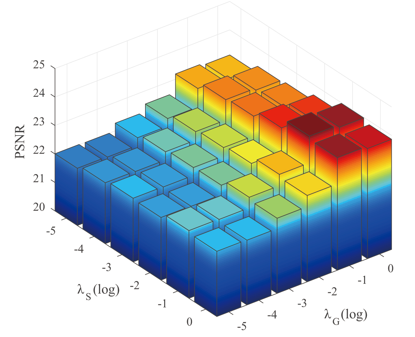
Figure 5: An ablation experiment of $\lambda_{G}$ and $\lambda_{S}$ over BSD300 dataset($\times 8$).

The main point in Fig. 5 to note is that MGE has a greater effect on PSNR than SSIM. A reliable explanation is that they have serious homogeneity because SSIM and MSE are both in the RGB domain, but MGE is in the gradient domain and provides a cross-domain information. Under the guidance of the ablation experiment result, $\lambda_{G}$ is set to $0.1$ and $\lambda_{S}$ is set to $0.1$ in all subsequent experiments.

Table 3: Evaluation of Mix Loss on U-net and Dense U-net backbone over SET14, BSD300 and ICDAR2003 datasets

Scale=2
Method	Loss	SET14	BSD300	ICDAR2003
		PSNR/SSIM	PSNR/SSIM	PSNR/SSIM
UnetSR	MSE	26.7241/0.8889	29.4241/0.8832	35.8147/0.9307
UnetSR	MixE	27.1359/0.8974	29.6336/0.8898	36.0978/0.9364
DenseSR	MSE	27.4011/0.9027	29.4902/0.8851	35.9829/0.9325
DenseSR	MixE	27.7713/0.9106	29.9828/0.9009	36.2948/0.9382
Scale=4
Method	Loss	SET14	BSD300	ICDAR2003
		PSNR/SSIM	PSNR/SSIM	PSNR/SSIM
UnetSR	MSE	20.8891/0.6693	24.8332/0.6843	29.3374/0.8202
UnetSR	MixE	21.3520/0.6859	25.1819/0.7033	29.8233/0.8181
DenseSR	MSE	21.4532/0.7009	24.9723/0.6927	30.4351/0.8392
DenseSR	MixE	21.9932/0.7181	25.4017/0.7141	31.0083/0.8523
Scale=8
Method	Loss	SET14	BSD300	ICDAR2003
		PSNR/SSIM	PSNR/SSIM	PSNR/SSIM
UnetSR	MSE	16.7001/0.4093	21.9865/0.5231	25.7734/0.7105
UnetSR	MixE	16.9707/0.4177	22.2273/0.5254	25.8770/0.7148
DenseSR	MSE	18.9354/0.5752	24.0628/0.6591	29.0465/0.8051
DenseSR	MixE	19.5080/0.6158	24.4807/0.6637	29.5169/0.8357
The MSE and MixE are only applied for network training.
The MSE and MixE are independent of evaluation methods.

The evaluation of mix loss function on the backbone of Dense U-net in Table. 3 illustrates its effectiveness. The modification of loss function obtains a great improvement on PSNR in most instances, which manifests in approximately +0.8dB increment.

4.5 Comparison with the state-of-the-arts

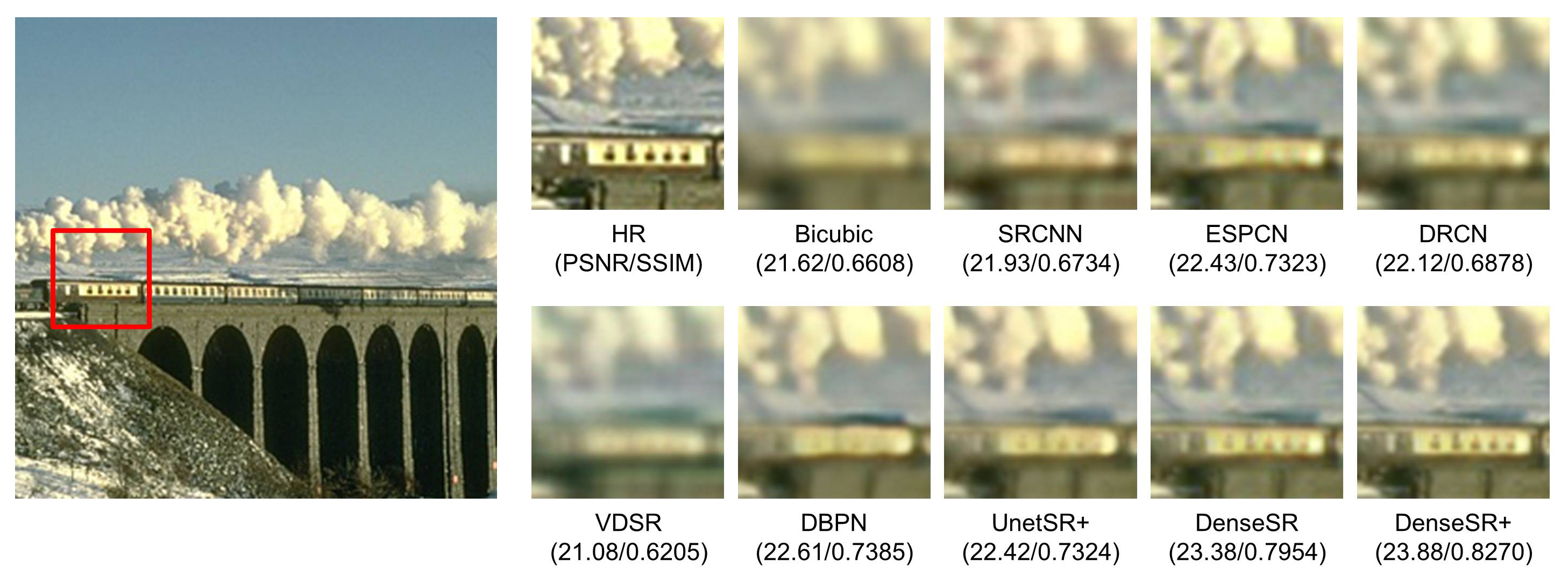
(a) Super-resolution results($4\times$) of 182053.jpg from BSD300 dataset

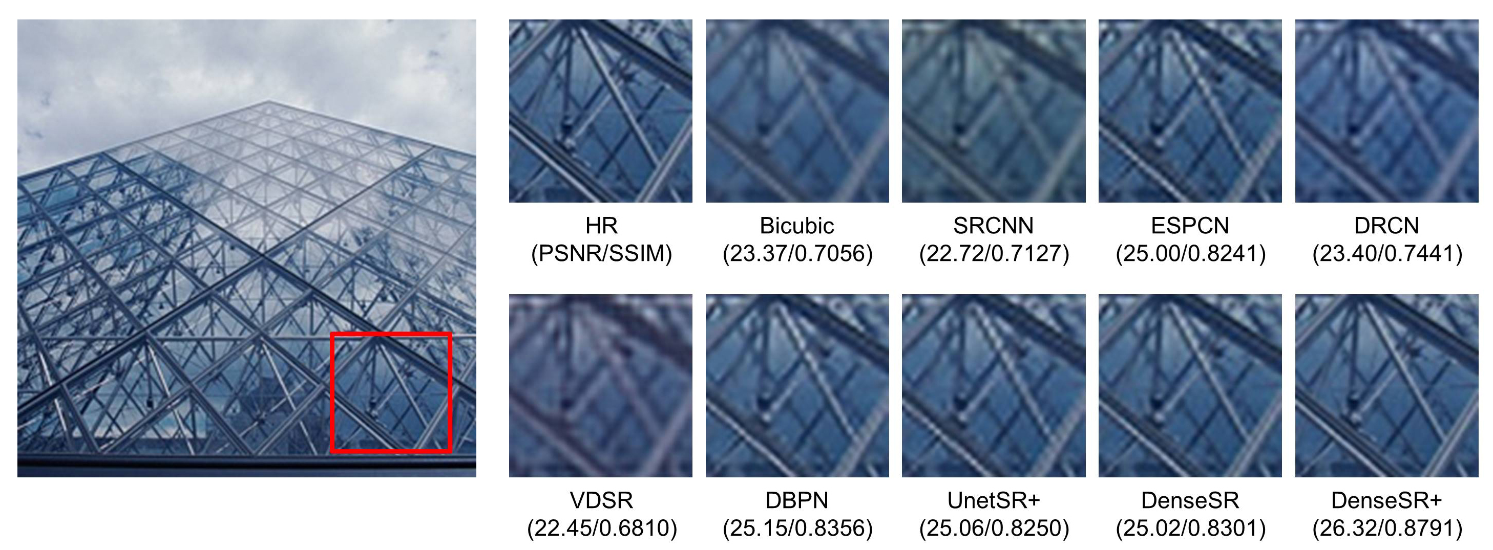
(b) Super-resolution results($2\times$) of 148026.jpg from BSD300 dataset

Figure 6: Reconstructed images by different methods.

The comparison between our method and previous works, includes ESPCNshi2016real , SRCNNdong2015image , VDSRkim2016accurate , EDSRlim2017enhanced , FSRCNNdong2016accelerating , DRCNkim2016deeply , SRGANledig2017photo , DBPNharis2018deep , RCANzhang2018image , SANdai2019second and Bicubicde1962bicubic , are shown as Table. 5 and Fig. 6(a)(b). In Table. 5, red numbers mark the highest score and blue numbers mark the second best results. It can be clear seen that the DenseSR+ performs the best under most circumstances. Table. 4 shows the comparison of parameter numbers and running time between different deep learning methods. Though DenseSR+ is a large parameter number deep learning method, it achieves the state-of-the-art performance.

Table 4: Comparison of PSNR and SSIM with the parameter number and running time

Scale=8
Method	Params	Time	BSD300	ICDAR2003
		(ms)	PSNR/SSIM	PSNR/SSIM
Bicubicde1962bicubic			21.3115/0.4933	24.3856/0.6831
ESPCNshi2016real	75552	1.2980	21.6447/0.5064	25.1132/0.6964
SRCNNdong2015image	171488	3.0600	21.8101/0.5075	22.6281/0.6103
VDSRkim2016accurate	224640	6.9120	21.9697/0.5181	25.6303/0.7104
EDSRlim2017enhanced	779523	16.540	21.6573/0.5067	23.5578/0.5987
FSRCNNdong2016accelerating	27267	0.8890	21.3311/0.5011	22.5721/0.6155
DRCNkim2016deeply	114307	60.5730	21.2771/0.4934	24.2561/0.6725
SRGANledig2017photo	6535494	12.0300	21.8766/0.5121	23.5621/0.6425
DBPNharis2018deep	23205878	82.5170	22.0577/0.5229	26.3482/0.7196
RCANzhang2018image	37129404	43.2140	22.5201/0.5712	29.3084/0.7928
SANdai2019second	30248124	106.3800	24.1560/0.6701	28.6021/0.7344
UnetSR lu2019single	8495907	16.9530	21.9865/0.5231	25.7734/0.7105
DenseSR	19109451	18.2470	24.0628/0.6591	29.0465/0.8051
DenseSR+	121352587	126.7016	25.5143/0.6874	30.6092/0.8413
Red numbers mark the best score.
Blue numbers mark the second best score.

Table 5: Comparison results on scale of 4

Scale=2
Method	SET14	BSD300	ICDAR2003
	PSNR/SSIM	PSNR/SSIM	PSNR/SSIM
Bicubicde1962bicubic	24.4523/0.8482	26.6538/0.7924	32.9327/0.9028
ESPCNshi2016real	26.7606/0.8999	28.9832/0.8732	35.6041/0.9243
SRCNNdong2015image	25.9711/0.8681	28.6943/0.8671	35.2711/0.9234
VDSRkim2016accurate	28.6617/0.9269	29.3889/0.8785	36.2323/0.9375
EDSRlim2017enhanced	24.0624/0.8383	28.3119/0.8621	34.5047/0.9258
FSRCNNdong2016accelerating	23.1284/0.8123	28.7534/0.8681	35.0533/0.9355
DRCNkim2016deeply	24.4234/0.8458	27.5089/0.8088	33.7849/0.9185
SRGANledig2017photo	23.9553/0.8195	28.7072/0.8633	33.2834/0.9135
DBPNharis2018deep	28.4092/0.9202	29.8675/0.8834	36.2344/0.9401
RCANzhang2018image	28.9150/0.9271	29.7674/0.8878	36.8491/0.9377
SANdai2019second	28.9672/0.9298	29.9189/0.9005	36.8947/0.9387
UnetSR lu2019single	26.7241/0.8889	29.4241/0.8832	35.8147/0.9307
DenseSR	27.4011/0.9027	29.4902/0.8851	35.9829/0.9325
DenseSR+	29.1197/0.9331	30.2264/0.9086	37.4785/0.9487
Scale=4
Method	SET14	BSD300	ICDAR2003
	PSNR/SSIM	PSNR/SSIM	PSNR/SSIM
Bicubicde1962bicubic	19.7167/0.6089	23.5053/0.6157	28.1135/0.7875
ESPCNshi2016real	20.6292/0.6333	24.4899/0.6641	29.4861/0.8214
SRCNNdong2015image	20.5825/0.6288	24.2232/0.6597	28.1906/0.7661
VDSRkim2016accurate	21.4763/0.6991	24.7077/0.6816	30.5267/0.8321
EDSRlim2017enhanced	19.9784/0.6269	23.9192/0.6513	27.9723/0.7101
FSRCNNdong2016accelerating	19.3255/0.5941	24.2499/0.6599	28.0231/0.7652
DRCNkim2016deeply	19.7077/0.6078	23.3462/0.6132	27.7174/0.7764
SRGANledig2017photo	19.3877/0.5976	24.1675/0.6485	27.5605/0.7654
DBPNharis2018deep	21.7657/0.7171	25.0644/0.6967	29.8832/0.8224
RCANzhang2018image	21.7085/0.7160	25.4241/0.6976	30.8147/0.8407
SANdai2019second	21.9241/0.7240	25.9141/0.7401	29.7817/0.8121
UnetSR lu2019single	20.8891/0.6693	24.8332/0.6843	29.3374/0.8202
DenseSR	21.4532/0.7009	24.9723/0.6927	30.4351/0.8392
DenseSR+	22.2568/0.7292	25.9024/0.7386	32.0652/0.8829
Scale=8
Method	SET14	BSD300	ICDAR2003
	PSNR/SSIM	PSNR/SSIM	PSNR/SSIM
Bicubicde1962bicubic	16.1132/0.3673	21.3115/0.4933	24.3856/0.6831
ESPCNshi2016real	16.3441/0.3628	21.6447/0.5064	25.1132/0.6964
SRCNNdong2015image	16.3853/0.3614	21.8101/0.5075	22.6281/0.6103
VDSRkim2016accurate	16.7994/0.4095	21.9697/0.5181	25.6303/0.7104
EDSRlim2017enhanced	15.7257/0.3209	21.6573/0.5067	23.5578/0.5987
FSRCNNdong2016accelerating	14.5788/0.2541	21.3311/0.5011	22.5721/0.6155
DRCNkim2016deeply	16.1497/0.3685	21.2771/0.4934	24.2561/0.6725
SRGANledig2017photo	15.7133/0.3221	21.8766/0.5121	23.5621/0.6425
DBPNharis2018deep	16.7398/0.4122	22.0577/0.5229	26.3482/0.7196
RCANzhang2018image	18.7580/0.5425	22.5201/0.5712	29.3084/0.7928
SANdai2019second	19.0185/0.6315	24.1560/0.6701	28.6021/0.7344
UnetSR lu2019single	16.7001/0.4093	21.9865/0.5231	25.7734/0.7105
DenseSR	18.9354/0.5752	24.0628/0.6591	29.0465/0.8051
DenseSR+	20.9134/0.6746	25.5143/0.6874	30.6092/0.8213

5 Conclusion

To solve the problem of limitations caused by defects in the information transmission structure, we propose a Dense U-net with shuffle pooling layer for super-resolution tasks and it achieves the state-of-the-art result In this work. Compare with U-net ronneberger2015u for SISR, Dense U-net reduces the information transmission loss because the up-sampling block combines all down-sampling feature maps from all depth of contracting blocks. Then, a novel pooling method called shuffle pooling is designed for the Dense U-net, which can effectively replace the handcrafted filter in the SISR pipeline with more lossy down-sampling filters specifically trained for each feature map, whilst also reducing the information loss of the overall SISR operation. Furthermore, the mix loss function, which combined with Mean Square Error(MSE) huynh2008scope , Structural Similarity Index (SSIM) hore2010image and Mean Gradient Error(MGE) lu2019single , basically solves the perception loss and high-frequency information loss. In experiments, the proposed Dense UnetSR outperforms the state-of-the-art the SISR methods in SET14, BSD300, ICDAR2003 datasets, especially in the text tasks.

- (1) Dong, C., Loy, C.C., He, K., Tang, X.: Image super-resolution using deep convolutional networks. IEEE transactions on pattern analysis and machine intelligence 38(2), 295–307 (2015)
- (2) Kim, J., Kwon Lee, J., Mu Lee, K.: Accurate image super-resolution using very deep convolutional networks. In: Proceedings of the IEEE conference on computer vision and pattern recognition, pp. 1646–1654 (2016)
- (3) Kim, J., Kwon Lee, J., Mu Lee, K.: Deeply-recursive convolutional network for image super-resolution. In: Proceedings of the IEEE conference on computer vision and pattern recognition, pp. 1637–1645 (2016)
- (4) Haris, M., Shakhnarovich, G., Ukita, N.: Deep back-projection networks for super-resolution. In: Proceedings of the IEEE conference on computer vision and pattern recognition, pp. 1664–1673 (2018)
- (5) Ronneberger, O., Fischer, P., Brox, T.: U-net: Convolutional networks for biomedical image segmentation. In: International Conference on Medical image computing and computer-assisted intervention, pp. 234–241. Springer (2015)
- (6) Huynh-Thu, Q., Ghanbari, M.: Scope of validity of psnr in image/video quality assessment. Electronics letters 44(13), 800–801 (2008)
- (7) Hore, A., Ziou, D.: Image quality metrics: Psnr vs. ssim. In: 2010 20th International Conference on Pattern Recognition, pp. 2366–2369. IEEE (2010)
- (8) Lu, Z., Chen, Y.: Single image super resolution based on a modified u-net with mixed gradient loss. arXiv preprint arXiv:1911.09428 (2019)
- (9) Dong, C., Loy, C.C., Tang, X.: Accelerating the super-resolution convolutional neural network. In: European conference on computer vision, pp. 391–407. Springer (2016)
- (10) De Boor, C.: Bicubic spline interpolation. Journal of mathematics and physics 41(1-4), 212–218 (1962)
- (11) Shi, W., Caballero, J., Huszár, F., Totz, J., Aitken, A.P., Bishop, R., Rueckert, D., Wang, Z.: Real-time single image and video super-resolution using an efficient sub-pixel convolutional neural network. In: Proceedings of the IEEE conference on computer vision and pattern recognition, pp. 1874–1883 (2016)
- (12) He, K., Zhang, X., Ren, S., Sun, J.: Deep residual learning for image recognition. In: Proceedings of the IEEE conference on computer vision and pattern recognition, pp. 770–778 (2016)
- (13) Ledig, C., Theis, L., Huszár, F., Caballero, J., Cunningham, A., Acosta, A., Aitken, A., Tejani, A., Totz, J., Wang, Z., et al.: Photo-realistic single image super-resolution using a generative adversarial network. In: Proceedings of the IEEE conference on computer vision and pattern recognition, pp. 4681–4690 (2017)
- (14) Goodfellow, I., Pouget-Abadie, J., Mirza, M., Xu, B., Warde-Farley, D., Ozair, S., Courville, A., Bengio, Y.: Generative adversarial nets. In: Advances in neural information processing systems, pp. 2672–2680 (2014)
- (15) Lim, B., Son, S., Kim, H., Nah, S., Mu Lee, K.: Enhanced deep residual networks for single image super-resolution. In: Proceedings of the IEEE conference on computer vision and pattern recognition workshops, pp. 136–144 (2017)
- (16) Agustsson, E., Timofte, R.: Ntire 2017 challenge on single image super-resolution: Dataset and study. In: 2017 IEEE Conference on Computer Vision and Pattern Recognition Workshops (CVPRW) (2017)
- (17) Zhang, Y., Li, K., Li, K., Wang, L., Zhong, B., Fu, Y.: Image super-resolution using very deep residual channel attention networks. In: Proceedings of the European Conference on Computer Vision (ECCV), pp. 286–301 (2018)
- (18) Dai, T., Cai, J., Zhang, Y., Xia, S.T., Zhang, L.: Second-order attention network for single image super-resolution. In: Proceedings of the IEEE conference on computer vision and pattern recognition, pp. 11065–11074 (2019)
- (19) Kanopoulos, N., Vasanthavada, N., Baker, R.L.: Design of an image edge detection filter using the sobel operator. IEEE Journal of solid-state circuits 23(2), 358–367 (1988)
- (20) Karatzas, D., Shafait, F., Uchida, S., Iwamura, M., i Bigorda, L.G., Mestre, S.R., Mas, J., Mota, D.F., Almazan, J.A., De Las Heras, L.P.: Icdar 2013 robust reading competition. In: 2013 12th International Conference on Document Analysis and Recognition, pp. 1484–1493. IEEE (2013)
- (21) Bevilacqua, M., Roumy, A., Guillemot, C., Alberi-Morel, M.L.: Low-complexity single-image super-resolution based on nonnegative neighbor embedding (2012)
- (22) Martin, D., Fowlkes, C., Tal, D., Malik, J., et al.: A database of human segmented natural images and its application to evaluating segmentation algorithms and measuring ecological statistics. Iccv Vancouver: (2001)
- (23) Kingma, D.P., Ba, J.: Adam: A method for stochastic optimization. arXiv preprint arXiv:1412.6980 (2014)