ForestNet: Classifying Drivers of Deforestation in Indonesia using Deep Learning on Satellite Imagery

Jeremy Irvin ¹, Hao Sheng¹¹footnotemark: 1 ¹, Neel Ramachandran¹, Sonja Johnson-Yu¹
Sharon Zhou¹, Kyle Story², Rose Rustowicz², Cooper Elsworth²
Kemen Austin ³, Andrew Y. Ng²²footnotemark: 2 ¹
¹Stanford University, ²Descartes Labs, ³RTI International
{jirvin16,haosheng,neelr,sonjyu,sharonz}@cs.stanford.edu
{kyle,rose,cooper}@descarteslabs.com, kaustin@rti.org, ang@cs.stanford.edu Equal contribution.Equal contribution.

Abstract

Characterizing the processes leading to deforestation is critical to the development and implementation of targeted forest conservation and management policies. In this work, we develop a deep learning model called ForestNet to classify the drivers of primary forest loss in Indonesia, a country with one of the highest deforestation rates in the world. Using satellite imagery, ForestNet identifies the direct drivers of deforestation in forest loss patches of any size. We curate a dataset of Landsat 8 satellite images of known forest loss events paired with driver annotations from expert interpreters. We use the dataset to train and validate the models and demonstrate that ForestNet substantially outperforms other standard driver classification approaches. In order to support future research on automated approaches to deforestation driver classification, the dataset curated in this study is publicly available at https://stanfordmlgroup.github.io/projects/forestnet.

1 Introduction

The preservation of forests is crucial for preventing loss of biodiversity, managing air and water quality, and mitigating climate change [1, 2]. Forest loss in the tropics, which contributes to around 10% of annual global greenhouse gas emissions [3], must be reduced to decrease the potential for climate tipping points [4]. The direct drivers of tropical deforestation, or the specific activities which lead to forest cover loss, include natural events like wildfires, as well as human-induced land uses such as industrial and smallholder agricultural development [5]. Determining the extent to which these processes contribute to forest loss enables companies to fulfill their zero-deforestation commitments and helps decision-makers design, implement, and enforce targeted conservation and management policies [6, 7, 8, 9]. Indonesia has one of the highest rates of primary forest loss in the tropics that places it among the largest emitters of greenhouse gases worldwide [10]. Recent work using high-resolution satellite imagery to manually classify the direct drivers of forest loss in Indonesia provides critical information about the nationwide causes of deforestation [11]. Methods to automate driver classification would enable more spatially-broad and temporally-dense driver attribution with significant implications on forest conservation policies.

The growth in availability of high-resolution satellite imagery coupled with advancements in deep learning methods present opportunities to automatically derive geospatial insights at scale [12, 13]. Recently, convolutional neural networks (CNNs) have enabled a variety of satellite-image based applications, including extracting socioeconomic data for tracking poverty [14], classifying land use for urban planning [15], and identifying the locations of solar photovoltaics in the U.S. to support the adoption of solar electricity [16]. Prior work has developed decision-tree-based models and other machine learning techniques to automatically identify land-use conversion following deforestation [17, 18, 19, 20, 21, 22]. However, these methods do not leverage the complete contextual information provided by satellite imagery and heavily depend on data that is not widely available at high resolution.

Driver Class, N	Training	Validation	Test
Plantation	686	219	265
Smallholder Agriculture	556	138	207
Grassland/shrubland	143	47	85
Other	231	70	112
Overall	1,616	474	669

Table 1: Number of events per driver class in the training, validation, and test sets. Each class was created by combining driver categories from [11] as shown in Table A1 in the Appendix.

In this work, we train CNNs to identify the direct drivers (plantation, smallholder agriculture, grassland/shrubland, or other drivers) of primary forest loss using satellite imagery in Indonesia. This task is challenging to automate due to the heterogeneity of drivers within images and driver classes, the rapid evolution of landscapes over time, and the lack of expert-annotated data. We highlight three key technical developments that enable high classification performance on this task, including pre-training on a large land cover dataset that we curate, data augmentation using satellite revisits, and multi-modal fusion with auxiliary predictors to complement the satellite imagery. Our best model, called ForestNet, substantially outperforms standard driver classification approaches. All data used in this study is publicly available to support future research on forest loss driver classification.

2 Methods

2.1 Forest Loss Events and Driver Annotations

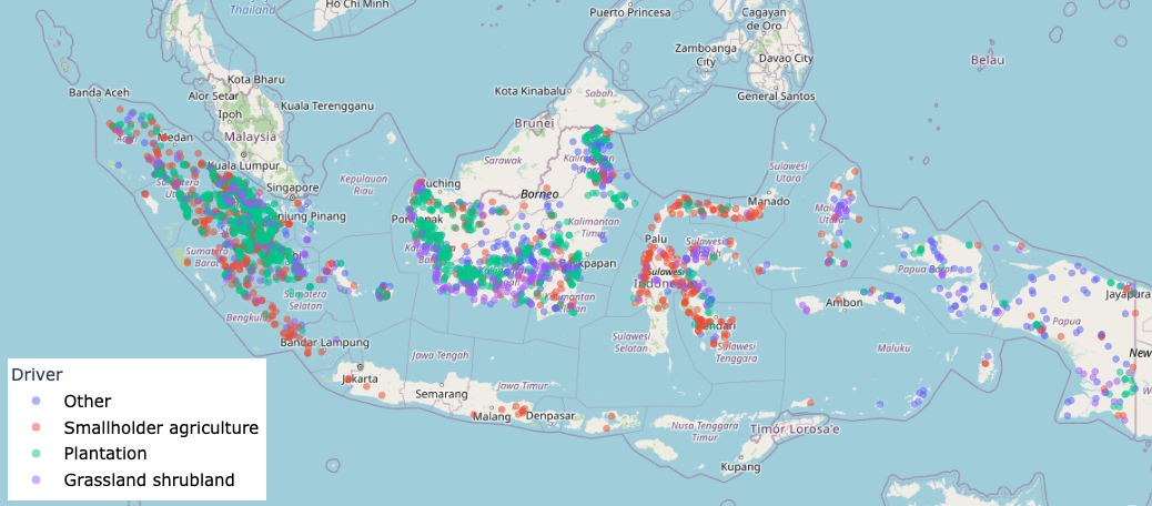
The coordinates of forest loss events and driver annotations used in this work were curated in [11]. Global Forest Change (GFC) published maps were used to obtain a random sample of primary natural forest loss events at 30m resolution from 2001 to 2016 [23]. Each forest loss region is represented as a polygon and is associated with a year indicating when the forest loss event occurred. An expert interpreter annotated each event with the direct driver of deforestation using high-resolution satellite imagery from Google Earth [11].

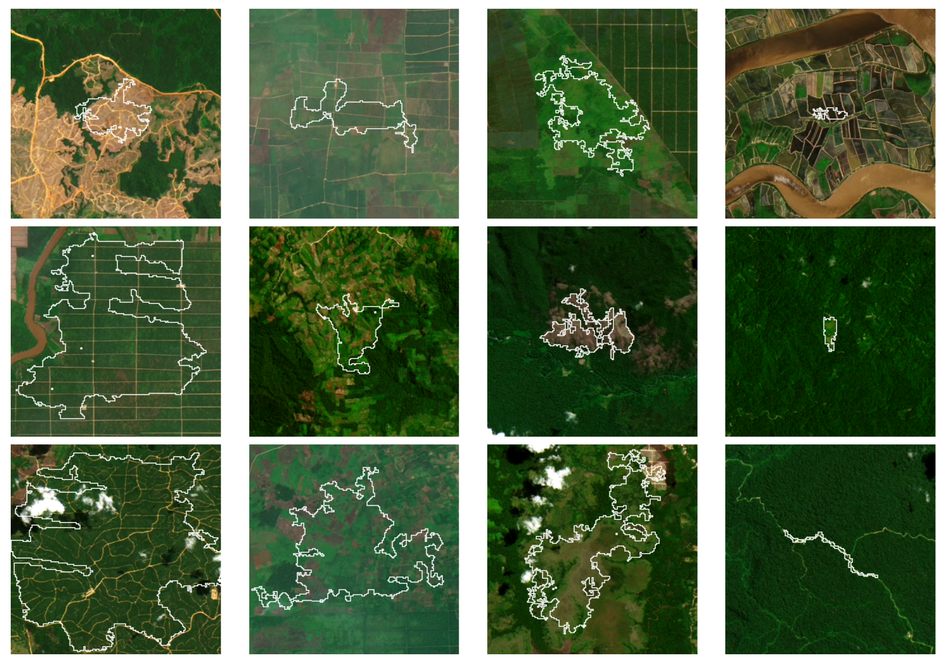
We group the drivers into categories that are feasible to differentiate using 15m resolution Landsat 8 imagery and to ensure sufficient representation of each category in the dataset. Due to the availability of Landsat 8 imagery starting in 2013 and challenges with constructing clear images with Landsat 7, we additionally remove any loss events before 2012 for driver classes that are likely to change over time [11]. Driver groupings and classes for which forest loss events before 2012 were dropped are shown in Table A1, and examples of each class are provided in Figure A1 in the Appendix.

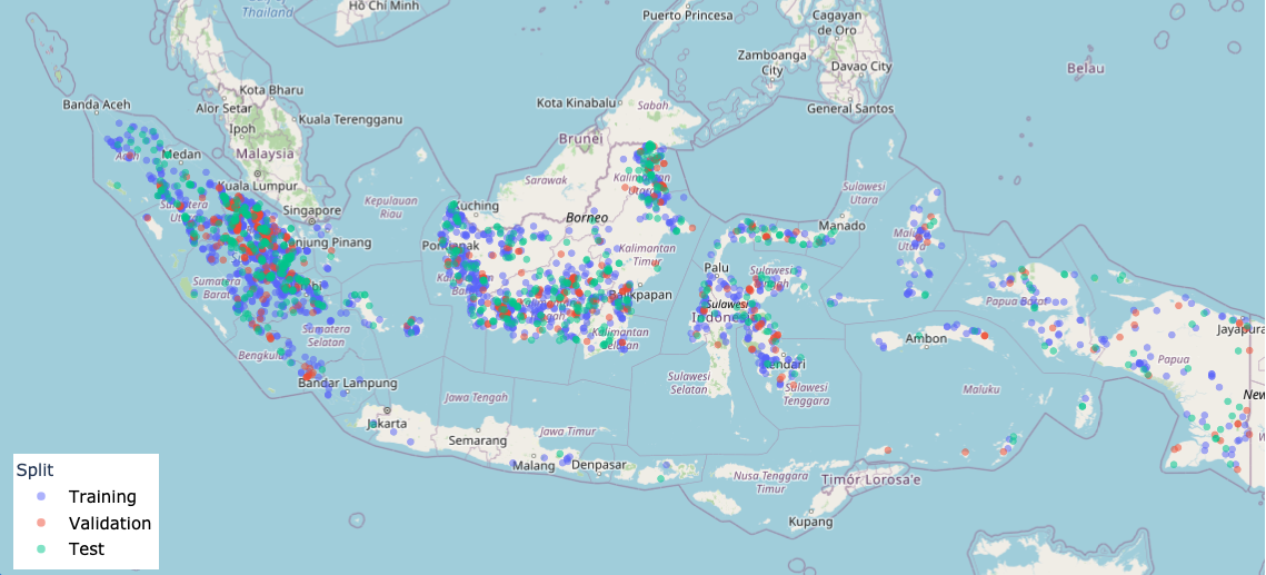
The complete dataset consists of 2,756 forest loss events with driver annotations. The dataset was randomly split into a training set to learn model parameters, a validation set to compare models, and a test set to evaluate the best model (Table 1, Figure A2). All examples in the validation and test sets were manually reviewed, and labels were corrected if the original label did not accurately represent the forest loss event by examination in high-resolution imagery using Google Earth.

2.2 Satellite Imagery

We capture each forest loss region with Tier 1 Landsat 8 satellite imagery acquired within five years of the event’s occurrence. All images are centered around the forest loss regions with visible bands pan-sharpened to 15m per-pixel resolution and a total size of 332 x 332 pixels, corresponding to an area of 5 square kilometers (500 hectares). Images for forest loss events occurring between 2012 and 2016 are captured during the four-year period starting the year after the event occurred (e.g., 2015-2018 for a 2014 event). Images for forest loss events occurring prior to 2012 are captured between 2013 and 2016 due to the availability of Landsat 8 imagery beginning in 2013. All images are converted to surface reflectance to account for atmospheric scattering or absorption.

We search for individual cloud-filtered scenes that capture the region of interest within the time range. We minimize cloud cover by only considering images with less than 50% cloudy pixels and 0% cirrus pixels according to the native Landsat 8 cloud and cirrus bands, respectively. We also construct a composite image by taking a per-pixel median over these cloud-filtered scenes, using the five least cloudy scenes when less than five such scenes were available. Using this procedure, we obtain exactly one composite image for each example and additional images for any individual cloud-filtered scenes.

2.3 Baseline Models and Auxiliary Predictors

Following recent work on automatically classifying land-use conversion from deforestation [17, 19], we develop random forest (RF) models that input a variety of variables including topographic, climatic, soil, accessibility, proximity, and spectral imaging predictors (Table A2). We additionally develop models which only input the Landsat 8 visible bands to assess the benefit of including the auxiliary variables. Details of the baseline models are provided in the Appendix.

2.4 ForestNet

Task. The deforestation driver classification task is to identify the direct driver of deforestation in a region of primary forest loss. Instead of a canonical multi-class classification approach, we formulate the task as semantic segmentation to (1) address that there are often multiple land uses within a single image, (2) implicitly utilize the information specific to the loss region, and (3) allow for high resolution (15m) predictions that can be used to predict different drivers for multiple loss regions of varying sizes. At train-time, we assign the single driver label to all of the pixels within the forest loss region. At test-time, the per-pixel model predictions in the forest loss region are used to obtain a single classification of the whole region, described below.

Architecture and Pre-Training. We experiment with a variety of segmentation architectures, including UNet [24], Feature Pyramid Networks [25], and DeepLabV3 [26]. For each segmentation architecture, we try several backbone architectures, including variants of ResNet [27], DenseNet [28], and EfficientNet [29]. We experiment with random weight initialization and pre-trained initialization learned from a large land cover dataset in Indonesia. We denote the use of pre-training as PT, and details of the training procedure, pre-training procedure, and loss functions are in the Appendix.

Refer to caption — Figure 1: ForestNet inputs a Landsat 8 satellite image centered around a region of forest loss and identifies the direct driver of forest loss in that region.

Data Augmentation. We experiment with several data augmentation techniques, including affine transformations, salt and pepper noise, and artificial clouds, haze, and fog [30]. We additionally randomly sample from the scenes and composite images during training to capture changes in landscape, which can occur in the same location due to seasonal differences, for example. We refer to this procedure as scene data augmentation (SDA). Images are randomly cropped to 160 x 160 pixels (approximately 2.4 x 2.4 km) during training, and center cropped to that size during prediction. No loss is computed for examples where the loss region is fully truncated due to cropping.

Multi-Modal Fusion with Auxiliary Variables. To leverage the auxiliary predictors in the deep learning models, we explore the use of multi-modal fusion [31, 32]. Specifically, we compute the mean, standard deviation, minimum, and maximum of the predictors in Table A2 within the forest loss region, concatenate them to the segmentation logits, then feed the result through three fully connected layers to obtain the class logits. We include ReLU and dropout after the first and second layers.

Driver Classification. The image captured temporally closest to the year of the forest loss event is input to the model at test-time to produce a per-pixel classification of the direct drivers within the forest loss region. The composite is used when no single scene meets the quality requirements. In order to convert the per-pixel logits within the forest loss region into a single classified driver, we compute the mean of the per-pixel scores in the polygon and make the predicted class the one assigned the highest score in the mean. For multi-modal fusion, the predicted class is the one assigned the highest score in the output of the final fully connected layer.

3 Results

Performance Measures on the Validation Set. The RF model that only inputs data from the visible Landsat 8 bands achieved the lowest performance on the validation set, but the incorporation of auxiliary predictors substantially improved its performance (Table 2 left). All of the CNN models outperformed the RF models. The best performing model, which we call ForestNet, used an FPN architecture with an EfficientNet-B2 backbone. The use of SDA provided large performance gains on the validation set, and land cover pre-training and incorporating auxiliary predictors each led to additional performance improvements.

Model	Predictors	Val		Test
Model	Predictors	Acc	F1	Acc	F1
RF	Visible	0.56	0.49	0.49	0.44
RF	Visible + Aux	0.72	0.67	0.67	0.62
CNN	Visible	0.80	0.75	0.78	0.70
CNN + SDA	Visible	0.82	0.79	0.78	0.73
CNN + SDA + PT	Visible	0.83	0.80	0.80	0.74
CNN + SDA + PT	Visible + Aux	0.84	0.81	0.80	0.75

Driver Category	P	R	F1
Plantation	0.81	0.92	0.86
Smallholder Agriculture	0.81	0.77	0.79
Grassland/shrubland	0.59	0.57	0.58
Other	0.90	0.70	0.79
Macro-average	0.78	0.74	0.75

Table 2: Accuracy and macro-average of the per-class F1 scores of the baseline and model variants on the validation set (left) and per-class performance metrics of ForestNet on the test set (right), including precision (P), recall (R), and F1-score. Validation results are reported as the average of 10 runs, and test results are reported for the best validation run.

Performance Measures on the Test Set. ForestNet achieved high classification performance across the four-driver categories on the test set (Table 2 right). The model achieved the best performance metrics on plantation and smallholder agriculture, which were the classes with the highest prevalence in the dataset. ForestNet performance on grassland/shrubland on the test set was the lowest primarily due to confusion with smallholder agriculture examples.

4 Discussion

We developed a deep learning model called ForestNet to automatically identify the direct drivers of primary forest loss in satellite images. To our knowledge, this is the first study to use deep learning for classifying the drivers of deforestation. A recent study has developed a semantic segmentation model for mapping industrial smallholder plantations, but is limited to closed-canopy oil palm and does not focus on land use directly after deforestation [33].

This study has important limitations that should be considered. First, ForestNet only leverages a single satellite image to make the classification, but the evolution of a landscape over time is important for identifying the direct driver [11]. Second, the model cannot differentiate between different species of plantations and types of smallholder agriculture development. Future work should explore the use of multiple high-resolution images to improve the accuracy and granularity of the driver predictions.

Our work contributes to the growing effort to use machine learning for tackling problems relevant to climate change [34]. ForestNet has the potential to generate accurate, temporally, and spatially dense maps of forest loss drivers over the entire nation of Indonesia. This new data could aid policymakers in developing more effective forest conservation and management policies to combat deforestation, one of the major contributors to global greenhouse gas emissions [3]. Focusing on forest loss in Indonesia is particularly important for climate change as the role of deforestation in its emissions profile is significantly larger than the rest of the world [35]. We hope that the methodology and data presented in this work eventually lead to comprehensive maps of forest loss drivers worldwide.

References

[1] J. A. Foley, R. DeFries, G. P. Asner, C. Barford, G. Bonan, S. R. Carpenter, F. S. Chapin, M. T. Coe, G. C. Daily, H. K. Gibbs, et al., “Global consequences of land use,” Science, vol. 309, no. 5734, pp. 570–574, 2005.
[2] J. A. Foley, N. Ramankutty, K. A. Brauman, E. S. Cassidy, J. S. Gerber, M. Johnston, N. D. Mueller, C. O’Connell, D. K. Ray, P. C. West, et al., “Solutions for a cultivated planet,” Nature, vol. 478, no. 7369, pp. 337–342, 2011.
[3] A. Arneth, F. Denton, F. Agus, A. Elbehri, K. Erb, B. Elasha, M. Rahimi, M. Rounsevell, A. Spence, and R. Valentini, “Ipcc special report on climate change,” Desertification, Land Degradation, Sustainable Land Management, Food Security, and Greenhouse gas fluxes in Terrestrial Ecosystems, 2019.
[4] T. M. Lenton, J. Rockström, O. Gaffney, S. Rahmstorf, K. Richardson, W. Steffen, and H. J. Schellnhuber, “Climate tipping points—too risky to bet against,” 2019.
[5] N. Hosonuma, M. Herold, V. De Sy, R. S. De Fries, M. Brockhaus, L. Verchot, A. Angelsen, and E. Romijn, “An assessment of deforestation and forest degradation drivers in developing countries,” Environmental Research Letters, vol. 7, no. 4, p. 044009, 2012.
[6] S. Donofrio, P. Rothrock, and J. Leonard, “Supply change: Tracking corporate commitments to deforestation-free supply chains,” Forest Trends, 2017.
[7] S. Henders, M. Ostwald, V. Verendel, and P. Ibisch, “Do national strategies under the un biodiversity and climate conventions address agricultural commodity consumption as deforestation driver?,” Land Use Policy, vol. 70, pp. 580–590, 2018.
[8] F. Seymour and N. L. Harris, “Reducing tropical deforestation,” Science, vol. 365, no. 6455, pp. 756–757, 2019.
[9] A. J. Hansen, P. Burns, J. Ervin, S. J. Goetz, M. Hansen, O. Venter, J. E. Watson, P. A. Jantz, A. L. Virnig, K. Barnett, et al., “A policy-driven framework for conserving the best of earth’s remaining moist tropical forests,” Nature Ecology & Evolution, pp. 1–8, 2020.
[10] K. G. Austin, N. L. Harris, A. Wijaya, D. Murdiyarso, T. Harvey, F. Stolle, and P. S. Kasibhatla, “A review of land-based greenhouse gas flux estimates in indonesia,” Environmental Research Letters, vol. 13, no. 5, p. 055003, 2018.
[11] K. G. Austin, A. Schwantes, Y. Gu, and P. S. Kasibhatla, “What causes deforestation in indonesia?,” Environmental Research Letters, vol. 14, no. 2, p. 024007, 2019.
[12] A. Karpatne, I. Ebert-Uphoff, S. Ravela, H. A. Babaie, and V. Kumar, “Machine learning for the geosciences: Challenges and opportunities,” IEEE Transactions on Knowledge and Data Engineering, vol. 31, no. 8, pp. 1544–1554, 2018.
[13] K. Janowicz, S. Gao, G. McKenzie, Y. Hu, and B. Bhaduri, “Geoai: spatially explicit artificial intelligence techniques for geographic knowledge discovery and beyond,” 2020.
[14] N. Jean, M. Burke, M. Xie, W. M. Davis, D. B. Lobell, and S. Ermon, “Combining satellite imagery and machine learning to predict poverty,” Science, vol. 353, no. 6301, pp. 790–794, 2016.
[15] A. Albert, J. Kaur, and M. C. Gonzalez, “Using convolutional networks and satellite imagery to identify patterns in urban environments at a large scale,” in Proceedings of the 23rd ACM SIGKDD international conference on knowledge discovery and data mining, pp. 1357–1366, 2017.
[16] J. Yu, Z. Wang, A. Majumdar, and R. Rajagopal, “Deepsolar: A machine learning framework to efficiently construct a solar deployment database in the united states,” Joule, vol. 2, no. 12, pp. 2605–2617, 2018.
[17] D. R. Richards and D. A. Friess, “Rates and drivers of mangrove deforestation in southeast asia, 2000–2012,” Proceedings of the National Academy of Sciences, vol. 113, no. 2, pp. 344–349, 2016.
[18] P. G. Curtis, C. M. Slay, N. L. Harris, A. Tyukavina, and M. C. Hansen, “Classifying drivers of global forest loss,” Science, vol. 361, no. 6407, pp. 1108–1111, 2018.
[19] D. Phiri, J. Morgenroth, and C. Xu, “Long-term land cover change in zambia: An assessment of driving factors,” Science of The Total Environment, vol. 697, p. 134206, 2019.
[20] A. Descals, Z. Szantoi, E. Meijaard, H. Sutikno, G. Rindanata, and S. Wich, “Oil palm (elaeis guineensis) mapping with details: Smallholder versus industrial plantations and their extent in riau, sumatra,” Remote Sensing, vol. 11, no. 21, p. 2590, 2019.
[21] A. Poortinga, K. Tenneson, A. Shapiro, Q. Nquyen, K. San Aung, F. Chishtie, and D. Saah, “Mapping plantations in myanmar by fusing landsat-8, sentinel-2 and sentinel-1 data along with systematic error quantification,” Remote Sensing, vol. 11, no. 7, p. 831, 2019.
[22] M. G. Hethcoat, D. P. Edwards, J. M. Carreiras, R. G. Bryant, F. M. Franca, and S. Quegan, “A machine learning approach to map tropical selective logging,” Remote sensing of environment, vol. 221, pp. 569–582, 2019.
[23] M. C. Hansen, P. V. Potapov, R. Moore, M. Hancher, S. A. Turubanova, A. Tyukavina, D. Thau, S. Stehman, S. J. Goetz, T. R. Loveland, et al., “High-resolution global maps of 21st-century forest cover change,” science, vol. 342, no. 6160, pp. 850–853, 2013.
[24] O. Ronneberger, P. Fischer, and T. Brox, “U-net: Convolutional networks for biomedical image segmentation,” in International Conference on Medical image computing and computer-assisted intervention, pp. 234–241, Springer, 2015.
[25] T.-Y. Lin, P. Dollár, R. Girshick, K. He, B. Hariharan, and S. Belongie, “Feature pyramid networks for object detection,” in Proceedings of the IEEE conference on computer vision and pattern recognition, pp. 2117–2125, 2017.
[26] L.-C. Chen, G. Papandreou, F. Schroff, and H. Adam, “Rethinking atrous convolution for semantic image segmentation,” arXiv preprint arXiv:1706.05587, 2017.
[27] K. He, X. Zhang, S. Ren, and J. Sun, “Deep residual learning for image recognition,” in Proceedings of the IEEE conference on computer vision and pattern recognition, pp. 770–778, 2016.
[28] G. Huang, Z. Liu, L. Van Der Maaten, and K. Q. Weinberger, “Densely connected convolutional networks,” in Proceedings of the IEEE conference on computer vision and pattern recognition, pp. 4700–4708, 2017.
[29] M. Tan and Q. V. Le, “Efficientnet: Rethinking model scaling for convolutional neural networks,” arXiv preprint arXiv:1905.11946, 2019.
[30] A. B. Jung, K. Wada, J. Crall, S. Tanaka, J. Graving, C. Reinders, S. Yadav, J. Banerjee, G. Vecsei, A. Kraft, Z. Rui, J. Borovec, C. Vallentin, S. Zhydenko, K. Pfeiffer, B. Cook, I. Fernández, F.-M. De Rainville, C.-H. Weng, A. Ayala-Acevedo, R. Meudec, M. Laporte, et al., “imgaug.” https://github.com/aleju/imgaug, 2020. Online; accessed 01-Feb-2020.
[31] P. K. Atrey, M. A. Hossain, A. El Saddik, and M. S. Kankanhalli, “Multimodal fusion for multimedia analysis: a survey,” Multimedia systems, vol. 16, no. 6, pp. 345–379, 2010.
[32] H. Sheng, X. Chen, J. Su, R. Rajagopal, and A. Ng, “Effective data fusion with generalized vegetation index: Evidence from land cover segmentation in agriculture,” in Proceedings of the IEEE/CVF Conference on Computer Vision and Pattern Recognition (CVPR) Workshops, June 2020.
[33] A. Descals, S. Wich, E. Meijaard, D. L. Gaveau, S. Peedell, and Z. Szantoi, “High-resolution global map of smallholder and industrial closed-canopy oil palm plantations,” Earth System Science Data Discussions, pp. 1–22, 2020.
[34] D. Rolnick, P. L. Donti, L. H. Kaack, K. Kochanski, A. Lacoste, K. Sankaran, A. S. Ross, N. Milojevic-Dupont, N. Jaques, A. Waldman-Brown, et al., “Tackling climate change with machine learning,” arXiv preprint arXiv:1906.05433, 2019.
[35] R. of Indonesia, “Indonesia’s third national communication under the united nations framework convention on climate change,” tech. rep., Ministry of Environment and Forestry, Jakarta, Indonesia, 2017.
[36] NASA JPL, “Nasa shuttle radar topography mission global 1 arc second.” https://lpdaac.usgs.gov/products/srtmgl1v003/, 2013. Online; accessed 28-Sep-2020.
[37] S. Saha, S. Moorthi, X. Wu, J. Wang, S. Nadiga, P. Tripp, D. Behringer, Y.-T. Hou, H. ya Chuang, M. Iredell, M. Ek, J. Meng, R. Yang, M. P. Mendez, H. van den Dool, Q. Zhang, W. Wang, M. Chen, and E. Becker, “The NCEP climate forecast system version 2,” Journal of Climate, vol. 27, pp. 2185–2208, Mar. 2014.
[38] World Resources Institute, “Peat lands.” https://data.globalforestwatch.org/datasets/d52e0e67ad21401cbf3a2c002599cf58_10. Online; accessed 28-Sep-2020.
[39] OpenStreetMap contributors, “Planet dump retrieved from https://planet.osm.org .” https://www.openstreetmap.org, 2017.
[40] Earth Resources Observation And Science (EROS) Center, “Collection-1 landsat 8 oli (operational land imager) and tirs (thermal infrared sensor) data products,” 2018.
[41] T.-Y. Lin, P. Goyal, R. Girshick, K. He, and P. Dollár, “Focal loss for dense object detection,” in Proceedings of the IEEE international conference on computer vision, pp. 2980–2988, 2017.
[42] C. H. Sudre, W. Li, T. Vercauteren, S. Ourselin, and M. J. Cardoso, “Generalised dice overlap as a deep learning loss function for highly unbalanced segmentations,” in Deep learning in medical image analysis and multimodal learning for clinical decision support, pp. 240–248, Springer, 2017.
[43] B. A. Margono, A. B. Usman, R. A. Sugardiman, et al., “Indonesia’s forest resource monitoring,” Indonesian Journal of Geography, vol. 48, no. 1, pp. 7–20, 2016.
[44] Global Forest Watch, “Land cover indonesia.” https://data.globalforestwatch.org/datasets/b1126d52d6c5416496339aeb250d9b39. Online; accessed 02-Oct-2020.

Appendix

Dataset

Driver Group	Driver Category	Drop Pre-2012
Plantation	Oil palm plantation	No
	Timber plantation	No
	Other large-scale plantations	No
Grassland/shrubland	Grassland/shrubland	Yes
Smallholder Agriculture	Small-scale agriculture	No
	Small-scale mixed plantation	No
	Small-scale oil palm plantation	No
Other	Mining	No
	Fish pond	No
	Logging road	Yes
	Secondary forest	Yes
	Other	No

Table A1: The driver categories defined in [11] are merged into groups that are feasible to differentiate using 15m resolution Landsat 8 imagery and to ensure sufficient representation of each category in the dataset. We additionally remove any loss events before 2012 for driver classes that are likely to change over time [11].

Predictor Group	Predictor (units)	Spatial	Temporal	Source	References
Predictor Group	Predictor (units)	Resolution	Resolution	Source	References
Topographic	Elevation (m)	30m	N/A	USGS (SRTM)	[36]
	Slope (0.01^∘)
	Aspect (0.01^∘)
Climatic	Surface-Level Albedo (0.01%)	56km	1 day	NCEP (CFSv2)	[37]
	Clear-Sky Longwave Flux (W/m²)
	Clear-Sky Solar Flux (W/m²)
	Direct Evaporation from Bare Soil (W/m²)
	Longwave Radiation Flux (W/m²)
	Shortwave Radiation Flux (W/m²)
	Ground Heat Net Flux (W/m²)
	Latent Heat Net Flux (W/m²)
	Specific Humidity ( $10^{-4}$ kg/kg)
	Potential Evaporation Rate (W/m²)
	Ground-Level Precipitation (0.1 mm)
	Sensible Heat Net Flux (W/m²)
	Volumetric Soil Moisture Content (0.01%)
	Air Pressure at Surface Level (10 Pa)
	Wind Components 10m above Ground (0.01 m/s)
	Water Runoff at Surface Level (0.01 kg/m²)
Soil	Presence of Peat	N/A	N/A	GFW (MoA)	[38]
Accessibility	Euclidean Distance to Road (km)	N/A	N/A	Open Street Map	[39]
Proximity	Euclidean Distance to City (km)	N/A	N/A	Open Street Map	[39]
Imaging	Landsat 8 Visible	15m	16 days	USGS (Landsat 8)	[40]
	Landsat 8 IR	30m
	Landsat 8 NDVI	30m

Table A2: The baseline models incorporate a variety of predictors that are commonly used in automatic methods for classifying land use. The climatic predictors were aggregated over the five years before the event using a mean, minimum, and maximum over the daily values. The imaging predictors were aggregated using the procedure to construct images with minimal cloud cover. All other predictors were measured at a single point in time.

Baseline Model Details

Model	Predictors	Val		Test
Model	Predictors	Acc	F1	Acc	F1
Logistic Regression Classifier	Visible	0.58	0.39	0.52	0.39
Logistic Regression Classifier	Visible + Aux	0.70	0.61	0.60	0.52
Ridge Regression Classifier	Visible	0.59	0.38	0.50	0.33
Ridge Regression Classifier	Visible + Aux	0.70	0.58	0.62	0.51
K-nearest Neighbor	Visible	0.53	0.39	0.46	0.33
K-nearest Neighbor	Visible + Aux	0.61	0.45	0.56	0.47
Multi-layer Perceptron	Visible	0.51	0.36	0.52	0.40
Multi-layer Perceptron	Visible + Aux	0.68	0.55	0.58	0.50
Decision Tree	Visible	0.40	0.38	0.37	0.37
Decision Tree	Visible + Aux	0.58	0.53	0.52	0.46
Random Forest	Visible	0.56	0.49	0.49	0.44
Random Forest	Visible + Aux	0.72	0.67	0.67	0.62

Table A3: Accuracy and macro-average of the per-class F1 scores of all baseline models on the validation and test sets.

We train multiple baseline models, including a decision tree, random forest, logistic regression classifier, ridge regression classifier, k-nearest neighbor classifier, and a multi-layer perceptron, and perform hyperparameter tuning using 3-fold cross-validation. For the tree-based models (decision tree and random forest), we tune the max depth of each tree, the minimum samples in leaves, and the number of decision trees. For the linear models (logistic regression classifier and ridge regression classifier), we tune the strength of regularization and the regularization norm (L1 or L2). For the k-nearest neighbor classifier, we tune the number of nearest neighbors. For the multi-layer perceptron model, we tune the number of hidden layers, the number of neurons in each hidden layer, and the learning rate.

We train two types of baseline models. The first type inputs and outputs data at 15m resolution, and all pixels within the loss regions in the training set were used as separate examples to train the model. Once the model was fit, a single driver classification over the full loss region is obtained from the model using the mode prediction over all pixels in the region. The second type of model inputs and outputs data corresponds to the forest loss region, where the per-pixel inputs are aggregated using a variety of statistics, including the mean, standard deviation, minimum, and maximum value of the variables within the region. The region-based model outperformed the pixel-based model, so we report the region-based model performance in Table 2 and Table A3.

CNN Loss Function

We experiment with a variety of segmentation losses, including cross entropy loss, focal loss [41], generalized dice loss [42], and a convex combination of focal and dice loss. Due to the heterogeneity of land use within a single image, we only compute segmentation loss on pixels within the forest loss region to avoid incorrect supervision on many pixels. We additionally include a cross-entropy loss that takes the mean of the forest loss region logits as input for the non-multi-modal models, and the output of the final fully connected layer for the multi-modal models. The final loss is a linear combination of the segmentation and classification losses.

CNN Training Procedure

For the CNN models, extensive hyperparameter tuning was performed over learning rate, architecture, backbone, data augmentation, regularization (dropout and weight decay), focal loss focusing parameter, coefficient of the convex combination in the segmentation loss, coefficient of the cross-entropy loss in the linear combination of the segmentation and classification loss, and batch size. During training, we evaluate the model on the validation set after each epoch and save the checkpoint with the highest F1 score averaged over the four-driver categories. All models were trained on a single NVIDIA TITAN-Xp GPU.

Pre-Training Details

We investigate the effect of randomly initializing the weights versus initializing the weights from models trained on a large land cover dataset. We pair Indonesia land cover categories manually classified by the Ministry of Environment Forestry in 2017 [43, 44] with Landsat 8 images created using the same procedure to minimize cloud cover described in the Satellite Imagery section. We include all tiles in Indonesia except for any tiles that overlapped with tiles in the driver dataset. The full dataset consists of 75,923 examples and is used to train the models for the pre-training experiments.