Subspace Recycling-based Regularization Methods

Abstract

Subspace recycling techniques have been used quite successfully for the acceleration of iterative methods for solving large-scale linear systems. These methods often work by augmenting a solution subspace generated iteratively by a known algorithm with a fixed subspace of vectors which are “useful” for solving the problem. Often, this has the effect of inducing a projected version of the original linear system to which the known iterative method is then applied, and this projection can act as a deflation preconditioner, accelerating convergence. Most often, these methods have been applied for the solution of well-posed problems. However, they have also begun to be considered for the solution of ill-posed problems.

In this paper, we consider subspace augmentation-type iterative schemes applied to linear ill-posed problems in a continuous Hilbert space setting, based on a recently developed framework describing these methods. We show that under suitable assumptions, a recycling method satisfies the formal definition of a regularization, as long as the underlying scheme is itself a regularization. We then develop an augmented subspace version of the gradient descent method and demonstrate its effectiveness, both on an academic Gaussian blur model and on problems arising from the adaptive optics community for the resolution of large sky images by ground-based extremely large telescopes.

68Q25, 68R10, 68U05

1 Introduction

This paper concerns the use of subspace recycling iterative methods in the context of solving linear ill-posed problems. There have already been a number of augmented or subspace recycling methods proposed specifically to treat ill-posed problems (e.g., [4, 3, 9, 5]), but these methods have yet to be formally analyzed as regularization schemes. More recently, an augmented scheme to accelerate the regularization of a problem in adaptive optics, producing a large improvement in performance, was proposed [32]. However, the augmentation was done after the regularized problem was set up rather than actually combining these techniques. It would thus be helpful to place all these methods into a common framework to streamline the development of new methods and to enable them to be analyzed using a common language and framework. In particular, it enables us in this paper to prove under what conditions augmented approaches described by the framework are regularizations.

We take advantage of a newly-proposed general framework [36] which can be used to describe the vast majority of these methods. This framework allows us to perform a general analysis of augmentation and recycling schemes as regularizations. From this, we develop sufficient conditions for a recycled iterative method to be a regularization, namely that a subspace recycling scheme is a regularization if it is built from an underlying regularization method. As a proof-of-concept, we then leverage the framework and our analysis to propose augmented steepest descent and Landweber methods, which we then apply to some test problems.

The linear inverse problem we consider is of the form

(1) $$Tx=y$$

whereby we approximately reconstruct $x$ from noisy data $y^{\delta}$ where $y^{\delta}=y+n$, and $n$ represents the perturbation of our data which satisfies $\|n\|\leq\delta$. Here, $T:{\mathcal{X}}\to{\mathcal{Y}}$ is a continuous mapping between separable Hilbert spaces ${\mathcal{X}},{\mathcal{Y}}$. In many relevant applications, the operator $T$ is ill-posed, i.e., (1) violates Hadamard’s conditions: a solution either might not exist, it might be non-unique or it may not depend continuously on the data. In this case regularization techniques have to be employed for the stable solution of (1), see [12, 13] and Section 2 for a summary on these methods.

The quality of the reconstruction for a specific problem depends heavily on available additional information on the solution, which is often directly included into the chosen reconstruction approach. E.g., source conditions of the solution are used to estimate the reconstruction error [13, 27]. Alternatively, information on the smoothness of the solution can be incorporated into Tikhonov regularization by choosing a penalty term that enforces the reconstruction to be smooth. For iterative regularization methods, the iteration can be started with a rough guess for the solution, leading generally to shorter reconstruction times and better results. Those approaches are of particular interest for inverse problems that have to be solved repeatedly in time and where the previous reconstruction can be considered as a good guess for the solution of the current problem. This would be the case, e.g., for Adaptive Optics applications in Astronomy, where the image quality loss due to turbulences in the atmosphere is corrected by a suitable shaped deformable mirror. The shape of the deformable mirrors has to be adjusted within milliseconds. The optimal shape of the mirror is derived by solving the atmospheric tomography problem repeatedly (about every 1-2ms). Although the atmosphere changes rapidly it can be regarded frozen on a sub-millisecond timescale, meaning that the previous reconstruction of the atmospheric tomography problem can be regarded as a good approximation to the new solution [40, 31].

In this paper we want to consider the case that we know a finite-dimensional subspace ${\mathcal{U}}\subset{\mathcal{X}}$ that contains a significant part of the solution $x^{\dagger}$ which we seek. As we will see, this part can be easily and stably be reconstructed. What then remains is to reconstruct the part that belongs to the orthogonal complement ${\mathcal{U}}^{\perp}$ of ${\mathcal{U}}$, possibly induces an acceleration in the convergence rate of the resulting iterative method, cf. Section 5.

For finite dimensional problems, this approach is known as a subspace recycling method and is currently a hot topic in numerical linear algebra. The goal of this paper is therefore to extend the theory to ill-posed problems in an infinite dimensional setting. Specifically, we will show that the concept of subspace recycling can be used in connection with most of the standard regularization methods.

The paper is organized as follows: In Section 2 we give a short introduction to Inverse Problems and regularization methods, whereas Section 3 discusses the state of research of subspace recycling methods. In Sections 4 and 5 we show that standard linear regularization method can be combined with subspace recycling and prove that the resulting method is still a regularization. Finally, Section 6 considers recycled gradient descent methods, and Section 7 presents some numerical results.

2 Regularization of linear ill-posed problems

We begin with a brief review of some basic regularization theory, which we mainly base on [12, 13, 27]. As mentioned above, a solution to the problem $Tx=y$ might not exist; if it exists it might not be unique and/or might not depend continuously on the data. The first two problems can be circumvented by using the generalized inverse $T^{\dagger}$, whereas stability is enforced by using regularization methods. To be more specific, an operator

(2) $$R_{\alpha}:Y\to X$$

is a regularization for a linear operator $T:X\to Y$ iff for any right hand side $y^{\delta}$ with $\|y-y^{\delta}\|\leq\delta$ there exists a parameter choice rule

(3) $$\alpha:\mathbb{R}\times Y\to\mathbb{R}^{+}$$

such that

(4) $$\lim_{\delta\to 0}R_{\alpha(\delta)}y^{\delta}=T^{\dagger}y=:x^{\dagger}$$

holds. Here, the parameter is chosen such that $\lim_{\delta\to 0}\alpha(\delta)=0$. Over the last decades, many regularization methods have been investigated, most prominently Tikhonov regularization and iterative methods like Landweber iteration [13, 24] and the conjugate gradient method. For Tikhonov regularization, the approximation $x_{\alpha}^{\delta}$ to the generalized solution $x^{\dagger}$ is computed as the minimizer of the Tikhonov functional

(5) $$J_{\alpha}(x)=\|y^{\delta}-Tx\|_{Y}^{2}+\alpha\Omega(x),$$

where $\Omega(x)$ is a suitable penalty term, e.g., $\Omega(x)=\|x\|^{2}$. For more general penalties we refer, e.g., to [12, 35]. For Tikhonov to be rendered a regularization method, one appropriate method of choosing the regularization parameter is the discrepancy principle, where $\alpha$ is chosen such that

(6) $$\|y^{\delta}-Tx_{\alpha}^{\delta}\|=\tau\delta,\hskip 28.45274pt\tau>1.$$

Iterative methods are popular as their computational realization is often straightforward. Landweber iteration computes as

(7) $$x_{k+1}^{\delta}=x_{k}^{\delta}+\beta T^{\ast}(y^{\delta}-Tx_{k}^{\delta}),\hskip 28.45274pt0<\beta<2/\|T\|^{2}.$$

For iterative methods the iteration index plays the role of the regularization parameter. According to the discrepancy principle, the iteration is terminated at step $k$ when for the first time $\|y^{\delta}-Tx_{k}^{\delta}\|\leq\tau\delta$ with $\tau>1$ fixed. The Landweber iteration with the discrepancy principle is a regularization method [13]. It is well known that the convergence of regularization methods for $\delta\to 0$ can be arbitrarily slow. Convergence rates can be obtained by using source conditions. Popular are Hölder type source conditions

(8) $$x^{\dagger}=(T^{\ast}T)^{\nu}w$$

for some $\mu\geq 0$ and $w\in X$. A regularization method is called order optimal iff the reconstruction error can be estimated as

(9) $$\|x^{\dagger}-R_{\alpha(\delta)}y^{\delta}\|=\mathcal{O}(\delta^{\nu/(\nu+1)})$$

provided a source condition (8) is fulfilled. Both Tikhonov and Landweber equipped with suitable source conditions are order optimal [13].

In this paper we will show that subspace recycling-based methods also form a regularization.

3 Augmented iterative methods

Augmented iterative methods, as we discuss them here, have been proposed in the literature beginning in the mid- to late-nineties; see [36] for a survey of this history. They can be considered as a specialized version of the class of iterative methods called residual constraint or residual projection methods. We discuss these methods briefly to put them into context, but for more details, the reader should see the survey paper [36], and references therein.

3.1 Iterations determined by residual constraint

Many iterative methods which are commonly used to treat both well- and ill-posed linear problems can be formulated according to a correction/constraint setup. Our discussion here in Section 3 focuses on the well-posed problem case for simplicity. Let $\left(\cdot,\cdot\right)_{{\mathcal{X}}}$ and $\left(\cdot,\cdot\right)_{{\mathcal{Y}}}$, respectively, be the inner products for ${\mathcal{X}}$ and ${\mathcal{Y}}$ and $\left(Tx,y\right)_{{\mathcal{X}}}=\left(x,T^{\ast}y\right)_{{\mathcal{Y}}}$.

Consider the case wherein we are solving Eq. 1 with no initial approximation; i.e., $x_{0}=0$. The strategies we outline here take the abstract form of approximating the solution $x^{\dagger}$ by $\hat{x}\in{\mathcal{S}}$ such that the residual satisfies $y-T\hat{x}\perp\widetilde{{\mathcal{S}}}$, where ${\mathcal{S}}\subset{\mathcal{X}}$ and $\widetilde{{\mathcal{S}}}\subset{\mathcal{Y}}$ are such that $\dim{\mathcal{S}}=\dim\widetilde{{\mathcal{S}}}<\infty$. They are called the correction and constraint spaces, respectively. A common example of a case for which $\dim{\mathcal{S}}=1$ is steepest descent (i.e., gradient descent with step size chosen to minimize the $T^{\ast}T$-norm of the error); see, e.g., [34, Section 5.3.1].

Proposition 3.1.

The $(j+1)$st step of steepest descent can be formulated as

(10) $$\mbox{\ \ \ select\ \ }t_{j+1}\in{\rm span}\left\{T^{\ast}r_{j}\right\}\mbox{\ \ \ such that\ \ }y-T\left(x_{j}+t_{j+1}\right)\perp{\rm span}\left\{TT^{\ast}r_{j}\right\},$$

where $r_{j}=y-Tx_{j}$; i.e., ${\mathcal{S}}={\rm span}\left\{T^{\ast}r_{j}\right\}$, and $\widetilde{{\mathcal{S}}}={\rm span}\left\{TT^{\ast}r_{j}\right\}$.

Proof 3.2.

Suppose we have constructed the approximation $x_{j}$ at the previous iteration. Recall that gradient descent methods compute $x_{j+1}=x_{j}+\alpha T^{\ast}r_{j}$, where $r_{j}=y-Tx_{j}$. The choice of $\alpha$ (called the step size) determines the method’s behavior. Steepest descent computes

$$\alpha_{j+1}=\underset{\alpha\in\mathbb{R}}{\text{{\rm argmin}}}\left\|y-T(x_{j}+\alpha T^{\ast}r_{j})\right\|_{{\mathcal{Y}}}.$$

Differentiating the right-hand side, setting it equal to zero, and solving for $\alpha_{j+1}$ yields the minimizer $\alpha_{j+1}=\dfrac{\left(r_{j},TT^{\ast}r_{j}\right)_{{\mathcal{Y}}}}{\left(TT^{\ast}r_{j},TT^{\ast}r_{j}\right)_{{\mathcal{Y}}}}$. One must simply show that Eq. 10 produces the same choice of $\alpha_{j+1}$. However, this constraint condition is equivalent to solving the equation

$$\left(r_{j}-\alpha_{j}TT^{\ast}r_{j},TT^{\ast}r_{j}\right)_{{\mathcal{Y}}}=0,$$

which when solved for $\alpha_{j}$ produces the same $T^{\ast}T$-norm-minimizing choice of $\alpha_{j}$.

Steepest descent is an example of a method for which $\dim{\mathcal{S}}=1$. There are many methods for which the size of the correction and constraint spaces grows at each iteration. It is a well-known result that one can characterize the method of conjugate gradients in this way, which we present without proof; see [33, 34] for proofs.

Proposition 3.3.

The $(j+1)$st iterate produced by the method of conjugate gradients applied to the normal equations associated to Eq. 1 can be formulated as

(11) $$\mbox{\ \ \ select\ \ }x_{j+1}\in{\mathcal{K}}_{j+1}\left(T^{\ast}T,T^{\ast}y\right)\mbox{\ \ \ such that\ \ }y-Tx_{j+1}\perp T{\mathcal{K}}_{j+1}\left(T^{\ast}T,T^{\ast}y\right),$$

where ${\mathcal{K}}_{j+1}\left(T^{\ast}T,T^{\ast}y\right)={\rm span}\left\{y,T^{\ast}Ty,\left(T^{\ast}T\right)^{2}y,\ldots,\left(T^{\ast}T\right)^{j}y\right\}$.

3.2 Augmentation via constraint over a pair of spaces

Many flavors of augmented iterative methods have been proposed to treat both well- and ill-posed problems. These methods treat the situation in which we wish to approximate the solution using an iterative method, but we also have a fixed subspace ${\mathcal{U}}$ which we also want to use to build the approximation. Using the correction/constraint formulation in Section 3.1, we can describe many of these methods as selecting approximations from a correction space ${\mathcal{S}}_{j}={\mathcal{U}}+{\mathcal{V}}_{j}\subset{\mathcal{X}}$ with a residual constraint space $\widetilde{{\mathcal{S}}}_{j}=\widetilde{{\mathcal{U}}}+\widetilde{{\mathcal{V}}}_{j}\subset{\mathcal{Y}}$, where ${\mathcal{U}}$ and $\widetilde{{\mathcal{U}}}$ are spaces of fixed dimension $k$ and ${\mathcal{V}}_{j}$ and $\widetilde{{\mathcal{V}}}_{j}$ are generated iteratively, with dimension $j$ at step $j$. It has been shown that this correction/constraint over the sum of subspaces reduces mathematically to applying the underlying iterative method to a projected problem, obtaining part of the approximation from ${\mathcal{V}}_{j}$ and then obtaining the corrections from ${\mathcal{U}}$ afterward. This will be explained in more detail in Section 5, but we give a brief outline here.

A projector is uniquely defined by its range and its null space. A standard result from linear algebra shows that this is equivalent to defining the ranges of the projector and its complement. In this setting, consider the projectors $P\in{\mathcal{L}}\left({\mathcal{X}}\right)$ and $Q\in{\mathcal{L}}\left({\mathcal{Y}}\right)$ having the relationship that

(12) $$TP=QT.$$

Let ${\rm Range}\left(P\right)={\mathcal{U}}$ and ${\rm Null}\left(P\right)=\left(T^{\ast}\,\widetilde{{\mathcal{U}}}\right)^{\perp}$, and ${\rm Range}\left(Q\right)=T\,{\mathcal{U}}$ and ${\rm Null}\left(Q\right)=\left(\widetilde{{\mathcal{U}}}\right)^{\perp}$. One can easily show that defining the null spaces is equivalent to defining ${\rm Range}\left(I_{{\mathcal{X}}}-P\right)=\left(T^{\ast}\,\widetilde{{\mathcal{U}}}\right)^{\perp}$ and ${\rm Range}\left(I_{{\mathcal{Y}}}-Q\right)=\widetilde{{\mathcal{U}}}^{\perp}$. For example, let $v\in{\mathcal{X}}$ be chosen arbitrarily. It can be decomposed as $v=v_{\mathcal{R}}+v_{\mathcal{N}}$ with $v_{\mathcal{R}}\in{\rm Range}\left(P\right)$ and $v_{\mathcal{N}}\in{\rm Null}\left(P\right)$. As expected, $Pv=Pv_{\mathcal{R}}+Pv_{\mathcal{N}}=v_{\mathcal{R}}$. We can then observe that $\left(I_{{\mathcal{X}}}-P\right)v=v_{\mathcal{R}}+v_{\mathcal{N}}-Pv_{\mathcal{R}}-Pv_{\mathcal{N}}=v_{\mathcal{N}}$. As $v\in{\mathcal{X}}$ was chosen arbitrarily, we see that ${\rm Range}\left(I_{{\mathcal{X}}}-P\right)={\rm Null}\left(P\right)$. The same can be shown for $Q$.

Approximating the solution of Eq. 1 by $x_{j}\in{\mathcal{S}}_{j}$ subject to the constraint $r_{j}\perp\widetilde{{\mathcal{S}}}_{j}$ has been shown to be equivalent to approximating the solution $t$ to the projected problem

(13) $$\left(I-Q\right)Tt=\left(I-Q\right)y$$

by $t_{j}\in{\mathcal{V}}_{j}$ with residual constraint space $\widetilde{{\mathcal{V}}}_{j}$ and setting the approximation $x_{j}\in{\mathcal{U}}+{\mathcal{V}}_{j}$ to be

(14) $$x_{j}=Px^{\dagger}+\left(I-P\right)t_{j};$$

see, [7] and [15, 16, 18].

For well-posed problems, the space ${\mathcal{U}}$ often contains vectors from previous iteration cycles applied to the current or previously-solved related problem; see, e.g., [2, 23, 29, 38]. These vectors are often (but not always) approximate eigenvectors (of a square operator) or left singular vectors, guided by Krylov subspace method convergence theory. For ill-posed problems, the strategy is generally to include some known features of the image/signal being reconstructed (see, e.g., [3, 4, 9]), but some current work by [5] still seeks to augment a Lanczos bidiagonalization-based solver for ill-posed, tall, skinny least-squares problems using approximate left singular vectors to accelerate semi-convergence and reduce the influence of smaller singular values to achieve a regularizing effect. See Section 5.1 for further discussion.

There is an alternative approach (originally proposed in the context of domain decomposition in, e.g., [14]) which begins with the projectors $P$ and $Q$ (rather than treating them as a consequence of the correction/constraint formulation) and produces the same algorithms but provides more flexibility to use methods like Landweber which do not have a clean residual constraint condition. This will be derived in detail in Section 5, but it is built on the simple idea that the projector $P$ can be used to get the decomposition $x^{\dagger}=Px^{\dagger}+\left(I-P\right)x^{\dagger}$. We will show that $Px^{\dagger}$ can be cheaply computed and we can use an iterative method to approximate $\left(I-P\right)x^{\dagger}$.

4 Linear Projection Methods

We consider here the case that $\widetilde{{\mathcal{U}}}=T\,{\mathcal{U}}$. For a finite dimensional subspace ${\mathcal{U}}\subset{\mathcal{X}}$ with $\dim{\mathcal{U}}=k>0$, we denote the sibling subspace ${\mathcal{C}}=T\,{\mathcal{U}}\subset{\mathcal{Y}}$ and assume it also has dimension $k$. We can represent these subspaces in terms of bases, which we denote with a matrix-like notation. Let

(15) $$\mathbf{U}=\begin{bmatrix}u_{1}&u_{2}&\cdots&u_{k}\end{bmatrix}\in{\mathcal{X}}^{k}\mbox{\ \ \ and\ \ \ }\mathbf{C}=\begin{bmatrix}c_{1}&c_{2}&\cdots&c_{k}\end{bmatrix}\in{\mathcal{Y}}^{k}$$

be $k$-tuples of elements from ${\mathcal{U}}$ and ${\mathcal{C}}$, respectively, which are bases for these spaces.

Remark 4.1.

To get a sense of these objects, observe that if ${\mathcal{X}}={\mathcal{Y}}=\mathbb{R}^{n}$ then we would have $\mathbf{U},\mathbf{C}\in\mathbb{R}^{n\times k}$; so this is just the generalization of the notion of a tall, skinny matrix.

We can consider $\mathbf{U}$ and $\mathbf{C}$ to be linear mappings induced by a basis expansion operation, with $\mathbf{U}\in{\mathcal{L}}\left(\mathbb{R}^{k},{\mathcal{X}}\right)$ and $\mathbf{C}\in{\mathcal{L}}\left(\mathbb{R}^{k},{\mathcal{Y}}\right)$, defined by

(16) $$\mathbf{U}\mathbf{z}=\sum_{i=1}^{k}z_{i}u_{i}\mbox{\ \ \ and\ \ \ }\mathbf{C}\mathbf{z}=\sum_{i=1}^{k}z_{i}c_{i}\mbox{\ \ \ for\ \ \ }\mathbf{z}=\ \begin{bmatrix}z_{1}&z_{2}&\cdots&z_{k}\end{bmatrix}^{T}\in\mathbb{R}^{k}.$$

Let

(17) $$\left(x,\mathbf{U}\right)_{{\mathcal{X}}}=\begin{bmatrix}\left(x,u_{1}\right)_{{\mathcal{X}}}\\ \vdots\\ \left(x,u_{k}\right)_{{\mathcal{X}}}\end{bmatrix}\in\mathbb{R}^{k},\mbox{\ \ \ and\ \ \ }\left(y,\mathbf{C}\right)_{{\mathcal{Y}}}=\begin{bmatrix}\left(y,c_{1}\right)_{{\mathcal{Y}}}\\ \vdots\\ \left(y,c_{k}\right)_{{\mathcal{Y}}}\end{bmatrix}\in\mathbb{R}^{k}.$$

Furthermore, for $\mathbf{M},\mathbf{L}\in{\mathcal{X}}^{k}$, we define the bilinear mapping

(18) $$\left(\cdot,\cdot\right)_{{\mathcal{X}}}:{\mathcal{X}}^{k}\times{\mathcal{X}}^{k}\rightarrow\mathbb{R}^{k\times k}\mbox{\ \ \ with\ \ \ }\left(\mathbf{M},\mathbf{L}\right)\mapsto\big{(}\left(m_{i},\ell_{j}\right)_{{\mathcal{X}}}\big{)}_{i,j=1}^{k}\in\mathbb{R}^{k\times k}.$$

We similarly define the corresponding bilinear mapping for two elements from $\mathbf{F},\mathbf{G}\in{\mathcal{Y}}^{k}$

$$\left(\cdot,\cdot\right)_{{\mathcal{Y}}}:{\mathcal{Y}}^{k}\times{\mathcal{Y}}^{k}\rightarrow\mathbb{R}^{k\times k}\mbox{\ \ \ with\ \ \ }\left(\mathbf{F},\mathbf{G}\right)\mapsto\big{(}\left(f_{i},g_{j}\right)_{{\mathcal{Y}}}\big{)}_{i,j=1}^{k}\in\mathbb{R}^{k\times k}.$$

In particular, we have the following relation:

Lemma 4.2.

For the operator $\mathbf{U}$ (and similarly $\mathbf{C}$) holds

(19) $$\|\mathbf{U}z\|_{{\mathcal{X}}}^{2}\leq\|(\mathbf{U},\mathbf{U})\|_{F}\|z\|^{2}_{\mathbb{R}^{k}}$$

Proof 4.3.

With $z=(z_{1},\dots,z_{k})\in\mathbb{R}^{k}$, $\mathbf{U}z=\sum_{i=1}^{k}z_{i}u_{j}\in{\mathcal{X}}$ follows

$$\|\mathbf{U}z\|^{2}_{{\mathcal{X}}} =\sum_{i=1}^{k}\sum_{j=1}^{k}z_{i}z_{j}\langle u_{i},u_{j}\rangle_{{\mathcal{X}}}$$

$$=\langle z,(\mathbf{U},\mathbf{U})z\rangle_{\mathbb{R}^{k}}\leq\|(\mathbf{U},\mathbf{U})z\|_{\mathbb{R}^{k}}\|z\|_{\mathbb{R}^{k}}$$

$$\leq\|(\mathbf{U},\mathbf{U})\|_{F}\|z\|^{2}_{\mathbb{R}^{k}}.$$

From Lemma 4.2 follows in particular

(20) $$\|\mathbf{U}\|_{\mathbb{R}^{k}\to{\mathcal{X}}}\leq\sqrt{\|(\mathbf{U},\mathbf{U})\|_{F}}.$$

We will further on also need

Lemma 4.4.

For $y\in{\mathcal{Y}}$ and $\mathbf{C}$ as above holds

(21) $$\|(y,\mathbf{C})\|_{\mathbb{R}^{k}}\leq\|T\|\|y\|_{\mathcal{Y}}\sqrt{\sum_{l=1}^{k}\|u_{l}\|^{2}}$$

Proof 4.5.

With (17) yields

(22) $$\|(y,\mathbf{C})\|_{\mathbb{R}^{k}}^{2} =\sum_{i=1}^{k}|(y,c_{i})_{\mathcal{Y}}|^{2}\leq\sum_{i=1}^{k}\|y\|^{2}_{\mathcal{Y}}\|c_{i}\|_{\mathcal{Y}}^{2}$$

(23) $$=\|y\|^{2}_{\mathcal{Y}}\sum_{i=1}^{k}\|Tu_{i}\|^{2}\leq\|T\|^{2}_{{}_{{\mathcal{X}}\to{\mathcal{Y}}}}\|\|y\|^{2}_{{\mathcal{Y}}}\sum_{i=1}^{k}\|u_{i}\|_{{\mathcal{X}}}^{2}$$

5 Projected Regularization Method

Let ${\mathcal{U}}\subset{\mathcal{X}}$ be a $k$-dimensional subspace, and ${\mathcal{C}}=T\,{\mathcal{U}}\subset{\mathcal{Y}}$ be its image under the action of $T$. Here it is important that we assume that the restricted operator $T|_{{\mathcal{U}}}$ is invertible, so as to guarantee that $\dim{\mathcal{U}}=\dim{\mathcal{C}}=k$ holds. This allows us express clearly the structure of projectors onto these spaces.

Proposition 5.1.

Assume that the vectors $u_{i}\in\mathbf{U}$ are linear independent, and that

(24) $$T_{|_{{\mathcal{U}}}}:{\mathcal{U}}\to Y$$

is invertible on its range $\mathcal{R}(T_{|_{{\mathcal{U}}}})$. Then $\left(\mathbf{C},\mathbf{C}\right)\in\mathbb{R}^{k\times k}$ is continuously invertible.

Proof 5.2.

According to (15), $\mathbf{C}=\begin{bmatrix}c_{1}&c_{2}&\cdots&c_{k}\end{bmatrix}\in{\mathcal{Y}}^{k}$ with $c_{i}=Tu_{i}$. As $T$ is invertible on $\mathcal{R}(T_{|_{{\mathcal{U}}}})$, the vectors in $\mathbf{C}$ are linear independent if the vectors in $\mathbf{U}$ are linear independent. Moreover,

(25) $$\left(\mathbf{C},\mathbf{C}\right)=\left(\left(c_{i},c_{j}\right)\right)_{i,j=1,\dots,k}$$

is the Gramian matrix of the linear independent system contained in $\mathbf{C}$ and therefore an invertible matrix. Additionally, as $\left(\mathbf{C},\mathbf{C}\right):\mathbb{R}^{k}\to\mathbb{R}^{k}$ maps between finite dimensional spaces, its inverse is also bounded.

In general, the operator $T$ is ill posed and might have a non-trivial null space, i.e., $T$ is not continuously invertible. However, on a finite dimensional subspace invertibility might be achieved easily.

Now let $Q$ be the ${\mathcal{Y}}$-orthogonal projector onto ${\mathcal{C}}$ and $P$ be the $\left(\cdot,T^{\ast}T\,\cdot\right)_{{\mathcal{X}}}$-orthogonal projector onto ${\mathcal{U}}$. The orthogonal projector $Q$ induces a direct sum splitting ${\mathcal{Y}}={\mathcal{C}}\oplus{\mathcal{C}}^{\perp_{\left(\cdot,\cdot\right)_{{\mathcal{Y}}}}}$. Consider $w\in{\mathcal{Y}}$. We represent the action of $Q$ as $Qw=\sum_{i=1}^{k}\left(w,c_{i}\right)_{{\mathcal{Y}}}c_{i}$. Similarly, $P$ induces a direct sum splitting of ${\mathcal{X}}$ with respect to $\left(\cdot,T^{\ast}T\,\cdot\right)_{{\mathcal{X}}}$, namely ${\mathcal{X}}={\mathcal{U}}\oplus{\mathcal{U}}^{\perp_{\left(\cdot,T^{\ast}T\,\cdot\right)_{{\mathcal{X}}}}}$ where ${\mathcal{U}}^{\perp_{\left(\cdot,T^{\ast}T\,\cdot\right)_{{\mathcal{X}}}}}$ denotes the orthogonal complement of ${\mathcal{U}}$ with respect to the inner product $\left(\cdot,T^{\ast}T\,\cdot\right)_{{\mathcal{X}}}$. We represent the action of $P$ as $Pv=\sum_{i=1}^{k}\left(v,T^{\ast}T\,u_{i}\right)_{{\mathcal{X}}}u_{i}$. We also can construct these projectors explicitly.

Proposition 5.3.

Let $\mathbf{U}\in{\mathcal{X}}^{k}$ be a basis of ${\mathcal{U}}$ and $\mathbf{C}=T\,\mathbf{U}\in{\mathcal{Y}}^{k}$ be a basis of ${\mathcal{C}}$. Then we have

$$P\cdot=\mathbf{U}\left(\mathbf{U},T^{\ast}T\,\mathbf{U}\right)_{{\mathcal{X}}}^{-1}\left(\cdot,T^{\ast}T\,\mathbf{U}\right)_{{\mathcal{X}}}\mbox{\ \ \ and\ \ \ }Q\cdot=\mathbf{C}\left(\mathbf{C},\mathbf{C}\right)_{{\mathcal{Y}}}^{-1}\left(\cdot,\mathbf{C}\right)_{{\mathcal{Y}}}.$$

Proof 5.4.

This is a standard result, particularly in the setting where ${\mathcal{X}}=\mathbb{R}^{m}$ and ${\mathcal{Y}}=\mathbb{R}^{n}$, but it is helpful to see why this is true in this more general setting, as well. From Proposition 5.1, we know that $\left(\mathbf{C},\mathbf{C}\right)=\left(T\mathbf{U},T\mathbf{U}\right)=\left(\mathbf{U},T^{\ast}T\mathbf{U}\right)$ is continuously invertible. Let $\left\{\hat{u}_{k+1},\hat{u}_{k+2},\ldots,\hat{u}_{\ell},\ldots\right\}$ be a basis for ${\mathcal{U}}^{\perp_{\left(\cdot,T^{\ast}T\,\cdot\right)_{{\mathcal{X}}}}}$. Then for any $v\in{\mathcal{X}}$, we can write

$$v=\sum_{i=1}^{k}\left(v,T^{\ast}T\,u_{i}\right)_{{\mathcal{X}}}u_{i}+\sum_{i=k+1}^{\infty}\left(v,T^{\ast}T\,\hat{u}_{i}\right)_{{\mathcal{X}}}\hat{u}_{i}.$$

Since by definition $\left(\hat{u_{i}},T^{\ast}T\,\mathbf{U}\right)_{{\mathcal{X}}}=0$ for all $i>k$, we can write

(26) $$\mathbf{U}\left(\mathbf{U},T^{\ast}T\,\mathbf{U}\right)_{{\mathcal{X}}}^{-1}\left(v,T^{\ast}T\,\mathbf{U}\right)_{{\mathcal{X}}}=\sum_{i=1}^{k}\left(v,T^{\ast}T\,u_{i}\right)_{{\mathcal{X}}}\mathbf{U}\left(\mathbf{U},T^{\ast}T\,\mathbf{U}\right)_{{\mathcal{X}}}^{-1}\left(u_{i},T^{\ast}T\,\mathbf{U}\right)_{{\mathcal{X}}}.$$

Observe that, according to the definitions in Eq. 17 and Eq. 18, the vector $\left(u_{i},T^{\ast}T\,\mathbf{U}\right)_{{\mathcal{X}}}$ is the $i$th column of the matrix $\left(\mathbf{U},T^{\ast}T\,\mathbf{U}\right)_{{\mathcal{X}}}$. Thus,

$$\left(\mathbf{U},T^{\ast}T\,\mathbf{U}\right)_{{\mathcal{X}}}^{-1}\left(u_{i},T^{\ast}T\,\mathbf{U}\right)_{{\mathcal{X}}}=\mathbf{e}_{i}\in\mathbb{R}^{k}$$

the $i$th Cartesian basis vector. Thus, we have

(27) $$\mathbf{U}\left(\mathbf{U},T^{\ast}T\,\mathbf{U}\right)_{{\mathcal{X}}}^{-1}\left(u_{i},T^{\ast}T\,\mathbf{U}\right)_{{\mathcal{X}}}=\mathbf{U}\mathbf{e}_{i}=u_{i}$$

and thus according to Eq. 26

(28) $$\mathbf{U}\left(\mathbf{U},T^{\ast}T\,\mathbf{U}\right)_{{\mathcal{X}}}^{-1}\left(v,T^{\ast}T\,\mathbf{U}\right)_{{\mathcal{X}}}=\sum_{i=1}^{k}\left(v,T^{\ast}T\,u_{i}\right)_{{\mathcal{X}}}u_{i}.$$

As $v$ was chosen arbitrarily, this is true for any element of ${\mathcal{X}}$ meaning the action of $\mathbf{U}\left(\mathbf{U},T^{\ast}T\,\mathbf{U}\right)_{{\mathcal{X}}}^{-1}\left(\cdot,T^{\ast}T\,\mathbf{U}\right)_{{\mathcal{X}}}$ is the action of $P$. This completes the proof for $P$. The same line of reasoning yields the proof for $Q$.

We assume that with exact data that Eq. 1 is consistent. Using the projector $P$, we decompose the exact true solution,

$$x^{\dagger}=Px^{\dagger}+\left(I_{{\mathcal{X}}}-P\right)x^{\dagger}.$$

With exact data, $Px^{\dagger}$ would be exactly computable, since we can rewrite

(29) $$x_{p}^{\dagger}:=Px^{\dagger}=\mathbf{U}\left(\mathbf{C},\mathbf{C}\right)_{{\mathcal{Y}}}^{-1}\left(Tx,\mathbf{C}\right)_{{\mathcal{Y}}}=\mathbf{U}\left(\mathbf{C},\mathbf{C}\right)_{{\mathcal{Y}}}^{-1}\left(y,\mathbf{C}\right)_{{\mathcal{Y}}}.$$

However, we do no have exact data. We have disturbed data $y^{\delta}$ such that $\left\|y-y^{\delta}\right\|_{{\mathcal{Y}}}\leq\delta$. Rewriting

(30) $$Px=\mathbf{U}\left(\mathbf{C},\mathbf{C}\right)_{{\mathcal{Y}}}^{-1}\left(y-y^{\delta},\mathbf{C}\right)_{{\mathcal{Y}}}+\mathbf{U}\left(\mathbf{C},\mathbf{C}\right)_{{\mathcal{Y}}}^{-1}\left(y^{\delta},\mathbf{C}\right)_{{\mathcal{Y}}}$$

we can define

(31) $$x_{p}^{\delta}:=\mathbf{U}\left(\mathbf{C},\mathbf{C}\right)_{{\mathcal{Y}}}^{-1}\left(y^{\delta},\mathbf{C}\right)_{{\mathcal{Y}}},$$

which can be computed inexpensively to high precision and may be used as an approximation $x_{p}^{\delta}\approx Px^{\dagger}$. We obtain

Proposition 5.5.

The approximation error between $x_{p}^{\dagger}$ and $x_{p}^{\delta}$ is given by

(32) $$x_{p}^{\dagger}-x_{p}^{\delta}=\mathbf{U}\left(\mathbf{C},\mathbf{C}\right)_{{\mathcal{Y}}}^{-1}\left(y-y^{\delta},\mathbf{C}\right)_{{\mathcal{Y}}},$$

which can be estimated as

(33) $$\left\|x_{p}^{\dagger}-x_{p}^{\delta}\right\|\leq\left(\sqrt{\|(\mathbf{U},\mathbf{U})\|_{F}\sum_{l=1}^{k}\|u_{l}\|^{2}}\left\|\left(\mathbf{C},\mathbf{C}\right)^{-1}\right\|_{F}\right)\delta.$$

Proof 5.6.

Using (29)-(31) gives (32), which can be estimated as

(34) $$\left\|x_{p}^{\dagger}-x_{p}^{\delta}\right\|_{{\mathcal{X}}} \leq\left\|\mathbf{U}\left(\mathbf{C},\mathbf{C}\right)_{{\mathcal{Y}}}^{-1}\left(y-y^{\delta},\mathbf{C}\right)_{{\mathcal{Y}}}\right\|$$

(35) $$\leq\left\|\mathbf{U}\right\|_{\mathbb{R}^{k}\to{\mathcal{X}}}\left\|\left(\mathbf{C},\mathbf{C}\right)^{-1}\right\|_{\mathbb{R}^{k}\to\mathbb{R}^{k}}\left\|\left(y-y^{\delta},\mathbf{C}\right)_{{\mathcal{Y}}}\right\|_{\mathbb{R}^{k}}$$

(36) $$\stackrel{{\scriptstyle\eqref{Unorm},\eqref{yC_est}}}{{\leq}}\sqrt{\|(\mathbf{U},\mathbf{U})\|_{F}}\left\|\left(\mathbf{C},\mathbf{C}\right)^{-1}\right\|_{\mathbb{R}^{k}\to\mathbb{R}^{k}}\|T\|\|y-y^{\delta}\|_{\mathcal{Y}}\sqrt{\sum_{l=1}^{k}\|u_{l}\|^{2}}$$

(37) $$=\left(\sqrt{\|(\mathbf{U},\mathbf{U})\|_{F}\sum_{l=1}^{k}\|u_{l}\|^{2}}\left\|\left(\mathbf{C},\mathbf{C}\right)^{-1}\right\|_{F}\right)\delta$$

Remark 5.7.

Often with such recycling methods, one takes either ${\mathcal{U}}$ or ${\mathcal{C}}$ to be represented with an orthonormal basis, for the purposes of convenience with regard to analysis and implementation. We assume here that ${\mathcal{C}}$ is represented by an orthonormal basis. If we scale $\mathbf{U}$ such that $\mathbf{C}=T\,\mathbf{U}$ is an orthonormal system spanning ${\mathcal{C}}$, we can write Eq. 33 more compactly as

$$\left\|Px-x_{p}^{\delta}\right\|_{{\mathcal{X}}}\leq\left\|\mathbf{U}\right\|_{{\mathcal{X}}}\delta={\mathcal{O}}\left(\delta\right).$$

Furthermore, $P$ and $Q$ can be expressed more compactly,

$$P\cdot=\mathbf{U}\left(\cdot,T^{\ast}T\,\mathbf{U}\right)_{{\mathcal{X}}}\mbox{\ \ \ and\ \ \ }Q\cdot=\mathbf{C}\left(\cdot,\mathbf{C}\right)_{{\mathcal{Y}}},$$

due to the fact that $\left(\mathbf{U},T^{\ast}T\,\mathbf{U}\right)_{{\mathcal{X}}}=\left(\mathbf{C},\mathbf{C}\right)_{{\mathcal{Y}}}=\mathbf{I}$ when $\mathbf{C}$ is an orthonormal system.

It remains to find a suitable approximation for $\left(I_{{\mathcal{X}}}-P\right)x^{\dagger}$. We have the following result:

Proposition 5.8.

Under the assumption

(38) $$QT(I-P)x^{\dagger}=0$$

holds

(39) $$y-y_{p}=(I-Q)T(I-P)x^{\dagger},$$

where

(40) $$y_{p}:=Tx_{p}^{\dagger}.$$

Proof 5.9.

We have

(41) $$y=Tx^{\dagger}=QTPx^{\dagger}+QT(I-P)x^{\dagger}+(I-Q)TPx^{\dagger}+(I-Q)T(I-P)x^{\dagger}.$$

As $x_{p}^{\delta}=Px^{\dagger}\in{\mathcal{U}}$ we have $y_{p}=Tx_{p}^{\delta}\in T{\mathcal{U}}$ and therefore

(42) $$y_{p}=Tx_{p}^{\delta}=QTPx^{\dagger}.$$

Further on, as $TPx^{\dagger}\in T{\mathcal{U}}$ and $(I-Q)$ projects onto the complement of $T{\mathcal{U}}$ we obtain

(43) $$(I-Q)TPx^{\dagger}=0.$$

Inserting (42), (43) into (41) yields

(44) $$y-y_{p}=QT(I-P)x^{\dagger}+(I-Q)T(I-P)x^{\dagger},$$

and Assumption (38) yields (39)

Assumption (38) transforms to

(45) $$QT(I-P)x^{\dagger}=0 \Longleftrightarrow \langle z,QT(I-P)x^{\dagger}\rangle=0\hskip 28.45274pt\forall z\in{\mathcal{Y}}$$

$$\Longleftrightarrow \langle T^{\ast}Qz,(I-P)x^{\dagger}\rangle=0\hskip 28.45274pt\forall z\in{\mathcal{Y}}$$

We arrive at

Proposition 5.10.

If

(46) $$T^{\ast}{\mathcal{C}}\perp(I-P)x^{\dagger},$$

then (38) holds. Particularly, (46) is fulfilled if

(47) $$T^{\ast}T{\mathcal{U}}\subset{\mathcal{U}}$$

holds.

Proof 5.11.

As $Q{\mathcal{Y}}={\mathcal{C}}$, eq. (45) transforms to (46). As $(I-P)x^{\dagger}\in{\mathcal{U}}^{\perp}$ holds always if we additionally assume that ${\mathcal{U}}$ is chosen s.t. $T^{\ast}{\mathcal{C}}\perp{\mathcal{U}}^{\perp}$, and with ${\mathcal{C}}=T{\mathcal{U}}$ this transforms to $T^{\ast}T{\mathcal{U}}\perp{\mathcal{U}}^{\perp}$ or, equivalently, (47).

Remark 5.12.

Obviously, (47) is much stronger than (46). However, there are easy examples where (46) always holds:

1. If ${\mathcal{U}}=span\{u_{i}:i=1,\dots N\mbox{ and }T^{\ast}Tu_{i}=\sigma_{i}u_{i}\}$ then clearly $T^{\ast}T{\mathcal{U}}\subset{\mathcal{U}}$.

2. If $T$ is an unitary operator, i.e., $\langle Tx_{1},Tx_{2}\rangle=\langle x_{1},x_{2}\rangle$ holds for all $x_{1},x_{2}$, then we have for $u\in{\mathcal{U}}$ and $u^{\perp}\in{\mathcal{U}}^{\perp}$

   $$\langle T^{\ast}Tu,u^{\perp}\rangle=\langle Tu,Tu^{\perp}\rangle=\langle u,u^{\perp}\rangle=0,$$

   i.e., (47).

Furthermore, the way we construct our projectors ensures that the assumption holds.

Lemma 5.13.

The assumption Eq. 38 holds for any pair of projectors $\left(P,Q\right)$ satisfying Eq. 12.

Proof.  This follows from the fact that the product of complementary projectors is the zero operator, since from Eq. 12, we have

$$QT(I-P)x^{\dagger}=Q(I-Q)Tx^{\dagger}=0.$$

     

With the above results we can now compute $(I-P)x^{\dagger}$ as a solution of equation (38). However, as always in Inverse Problems, we might not have the exact right hand side $y-y_{p}$ but some noisy version $y^{\delta}-y_{p}^{\delta}$, where we define $y_{p}^{\delta}:=Tx_{p}^{\delta}$. The data error can be approximated as follows:

Proposition 5.14.

The data error in the left hand side of (38) can be estimated as

(48) $$\|(y-y_{p})-(y^{\delta}-y_{p}^{\delta})\|\leq\kappa_{{\mathcal{U}}}\cdot\delta$$

with

(49) $$\kappa_{{\mathcal{U}}}:=1+\|T\|\sqrt{\|(\mathbf{U},\mathbf{U})\|_{F}\sum_{l=1}^{k}\|u_{l}\|^{2}}\left\|\left(\mathbf{C},\mathbf{C}\right)^{-1}\right\|_{F}$$

Proof 5.15.

The proof is straight forward:

(50) $$\|(y-y_{p})-(y^{\delta}-y_{p}^{\delta})\|\leq\|y-y^{\delta}\|+\|y_{p}-y_{p}^{\delta}\|\leq\delta+\|T\|\|x_{p}^{\dagger}-x_{p}^{\delta}\|$$

and with (33) follows (48)

We are now ready to formulate our solution approach:

1 Given:
$\bullet$ data $y^{\delta}$ fulfilling $\|y-y^{\delta}\|\leq\delta$
$\bullet$ ${\mathcal{U}}\subset{\mathcal{X}}$, ${\mathcal{U}}$ finite dimensional
$\bullet$ a regularization method $R_{\alpha}(y,T)$ for the equation $y=Tx$ with parameter choice rule $\alpha=\alpha(\delta)$

2 Compute $x_{p}^{\delta}$ according to (31) and set $y_{p}^{\delta}=Tx_{p}^{\delta}$

3 Set $B:=(I-Q)T$

4 Compute $\hat{x}_{p}^{\delta}:=R_{\alpha}(y^{\delta}-y_{p}^{\delta},B)$, $\alpha=\alpha(\kappa_{{\mathcal{U}}}\delta)$

Set $x_{{\mathcal{U}},\alpha}^{\delta}:=x_{p}^{\delta}+\hat{x}_{p}^{\delta}$

Algorithm 1 Augmented Regularization

Proposition 5.16.

If for the solution $x^{\dagger}$ of the equation $Tx=y$ and the chosen augmentation subspace ${\mathcal{U}}$ eq. (38) holds, then the augmented regularization with data $y^{\delta}$ fulfilling $\|y-y^{\delta}\|\leq\delta$ as described in Algorithm 1 forms a regularization method.

Proof 5.17.

As $R_{\alpha}(y^{\delta}-y_{p}^{\delta},B)$ is a regularization for (39) we have as $\delta\to 0$, and decomposing $x^{\dagger}=Px^{\dagger}+(I-P)x^{\dagger}=x_{p}^{\dagger}+\hat{x}_{p}^{\dagger}$ yields

$$\|x^{\dagger}-x_{{\mathcal{U}},\alpha}^{\delta}\| \leq \|x_{p}^{\dagger}-x_{p}^{\delta}\|+\|\hat{x}_{p}^{\dagger}-\hat{x}_{p}^{\delta}\|$$

$$\stackrel{{\scriptstyle\eqref{eqn.init-proj-err}}}{{\leq}} \mathcal{O}(\delta)+\|\hat{x}_{p}^{\dagger}-R_{\alpha(\kappa_{{\mathcal{U}}}\delta)}(y^{\delta}-y_{p}^{\delta},B)\|\stackrel{{\scriptstyle\delta\to 0}}{{\longrightarrow}}0$$

which concludes the proof.

Remark 5.18.

We can thus extend any existing regularization $R_{\alpha}$ to its augmented method and still obtain a regularization method.

Example 1.

Let us illustrate this for the Landweber method, which has been defined in (7). If the iteration is stopped by the discrepancy principle, i.e., if the stopping index $k_{\ast}$ is determined as the first index such that

(51) $$\|y^{\delta}-Tx_{k_{\ast}}^{\delta}\|\leq\tau\delta\hskip 28.45274pt\tau>1$$

holds, then it is a regularization method, see e.g., [8]. For given data $y^{\delta}$, the augmented Landweber method would read as

(52) $$x_{k_{\ast}}^{\delta}=x_{p}^{\delta}+\hat{x}_{k_{\ast}}^{\delta}$$

where $x_{p}^{\delta}$ is defined in (31) and $\hat{x}_{k_{\ast}}^{\delta}$ is the $k_{\ast}$th iterate of the Landweber iteration applied to the equation

(53) $$(I-Q)Tx=y^{\delta}-y_{p}^{\delta},\hskip 56.9055pty_{p}^{\delta}=Tx_{p}^{\delta}~{}.$$

Using

(54) $$y_{p}^{\delta}=Tx_{p}^{\delta}=T\mathbf{U}\left(\mathbf{C},\mathbf{C}\right)_{{\mathcal{Y}}}^{-1}\left(y^{\delta},\mathbf{C}\right)_{{\mathcal{Y}}}=\mathbf{C}\left(\mathbf{C},\mathbf{C}\right)_{{\mathcal{Y}}}^{-1}\left(y^{\delta},\mathbf{C}\right)_{{\mathcal{Y}}}=Qy^{\delta}$$

the iteration for $\hat{x}_{k}^{\delta}$ reads as

(55) $$\hat{x}_{k+1}^{\delta} = \hat{x}_{k}^{\delta}+T^{\ast}(I-Q)\left(y^{\delta}-y_{p}^{\delta}-(I-Q)T\hat{x}_{k}^{\delta}\right)$$

$$= \hat{x}_{k}^{\delta}+T^{\ast}(I-Q)\left(y^{\delta}-T\hat{x}_{k}^{\delta}\right).$$

Usually such an iteration is started with $\hat{x}_{0}^{\delta}=0$. Instead, we can incorporate $x_{p}^{\delta}$ directly into the iteration by setting $\hat{x}_{0}^{\delta}=x_{p}^{\delta}$.

5.1 What to recycle

One question we have not addressed thus far concerns what should the subspace ${\mathcal{U}}$ encode? This is a question that hinges very much on the application. Suffice it to say, a detailed review of recycling strategies is beyond the scope of this paper, but we refer the reader to [36, Section 6] for a more detailed discussion. Some common choices for augmentation vectors are approximate solutions or solutions to related problems, approximate or (when available) exact eigenvectors/singular vectors, and vectors satisfying convergence model optimality properties.

The use of approximate eigenvectors as a recycling strategy was first suggested for recycling between cycles of GMRES applied to one linear system to mitigate the effects on convergence speed of restarting [28]. The algorithmic choices in that paper necessitated that the approximate eigenvectors be harmonic Ritz vectors. Ritz-type eigenvector approximations with respect to a square matrix $\mathbf{A}$ are obtained applying a Galerkin or Petrov-Galerkin approximation strategy to the eigenvalue problem of the form

$$\mbox{select}\qquad\mathbf{v}\in\mathcal{V}\qquad\mbox{such that}\qquad\mathbf{A}\mathbf{v}-\lambda\mathbf{v}\perp\mathcal{W},$$

for some $\lambda\in\mathbb{R}$. The spaces $\mathcal{V}$ and $\mathcal{W}$ are usually spaces which have been generated during the iteration, so that the solution to the Ritz problem reduces to a (generalized) eigenvalue problem. This strategy was extended and combined with GCRO-type optimal methods in a way that did not require augmentation by harmonic Ritz vectors, and this enabled recycling between multiple linear systems [29]. This has been further extended to the case of short-recurrence schemes not requiring restart; see, e.g., [5, 23, 38]. In that case, one stores and updates a running recycle window but not to use in the current iteration. Rather, it is being built to be used in subsequent systems.

It should be noted that in the context of discrete ill-posed problems, a poor or noisy choice of ${\mathcal{U}}$ may induce a projected problem Eq. 13 which is even more ill-posed. However, it has been demonstrated that there are many good choices for ${\mathcal{U}}$; see, e.g., [3, 4, 9]. More recently, a recycled LSQR algorithm has been proposed where approximate eigenvectors are used as well as other data which become available in real-time [5]. As LSQR is a short-recurrence method, the authors employ a windowed recycling strategy, where the recycled subspace is updated every $p$ iterations so that only a window of vectors generated by the short recurrence iteration must be stored. They propose a few different recycling approaches appropriate for ill-posed problems: truncated singular vectors, solution- or sparsity-oriented compression, and reduced basis decomposition.

In the next section, we use the recycling method framework from [36] to develop augmented versions of steepest descent and Landweber methods. In Section 7, we combine this method with recycling strategies appropriate to each individual application, building on strategies from the literature but adjusted to fit the particular applications.

6 Augmented gradient descent methods

We now delve further into the case that we apply a gradient descent-type method (i.e., Landweber) to the projected problem, in order to produce a practical implementation of this algorithm. In particular, we first explore augmenting the steepest descent method, which can be understood as a Landweber-type method with a step-length that is dynamically chosen to minimize the residual norm. We have shown in Proposition 3.1 that this is a projection method and thus can be augmented in the above-discussed framework. Augmented methods such as this rely on certain identities to achieve algorithmic advantages.

Lemma 6.1.

The residual produced by the augmented iterative method with approximation $\hat{x}_{k}^{\delta}=\mathbf{U}\left(\mathbf{C},\mathbf{C}\right)_{{\mathcal{Y}}}^{-1}\left(y^{\delta},\mathbf{C}\right)_{{\mathcal{Y}}}+\left(I_{{\mathcal{X}}}-P\right)\hat{t}_{k}^{\delta}$ defined as in Eq. 14 where $\hat{t}_{k}^{\delta}$ is the approximate solution of Eq. 13 coincides with the residual associated to $\hat{t}_{k}^{\delta}$ for the projected problem Eq. 13, i.e.,

$$y^{\delta}-T\hat{x}_{k}^{\delta}=\left(I_{{\mathcal{Y}}}-Q\right)\left(y^{\delta}-T\hat{t}_{k}^{\delta}\right)\perp{\mathcal{C}}.$$

Proof.  This result has been shown in a number of papers for finite-dimensional, well-posed problems; see, [7] and [6, 15, 16, 18]. We show it here for completeness by direct calculation, by first writing

$$y^{\delta}-T\hat{x}_{j}^{\delta} =y^{\delta}-T\left(\mathbf{U}\left(\mathbf{C},\mathbf{C}\right)_{{\mathcal{Y}}}^{-1}\left(y^{\delta},\mathbf{C}\right)_{{\mathcal{Y}}}+\left(I_{{\mathcal{X}}}-P\right)\hat{t}_{j}^{\delta}\right)$$

$$y^{\delta}-T\hat{x}_{j}^{\delta} =y^{\delta}-\left(\mathbf{C}\left(\mathbf{C},\mathbf{C}\right)_{{\mathcal{Y}}}^{-1}\left(y^{\delta},\mathbf{C}\right)_{{\mathcal{Y}}}+T\left(I_{{\mathcal{X}}}-P\right)\hat{t}_{j}^{\delta}\right).$$

Then we observe that it follows from Proposition 5.3 and Eq. 12 that this is equivalent to

$$y^{\delta}-T\hat{x}_{j}^{\delta} =y^{\delta}-\left(Qy^{\delta}+\left(I_{{\mathcal{X}}}-Q\right)T\hat{t}_{j}^{\delta}\right)$$

$$=\left(I_{{\mathcal{X}}}-Q\right)y^{\delta}-\left(I_{{\mathcal{X}}}-Q\right)T\hat{t}_{j}^{\delta}.$$

It follows directly that $y^{\delta}-T\hat{x}_{j}^{\delta}\perp{\mathcal{C}}$.         Note that this proof holds in the presence or absence of noise and whether or not the problem being treated is consistent. In the case that the right-hand side is noise-free and the problem is consistent, we have from Eq. 30 that

(56) $$\mathbf{U}\left(\mathbf{C},\mathbf{C}\right)_{{\mathcal{Y}}}^{-1}\left(y,\mathbf{C}\right)_{{\mathcal{Y}}}=Px^{\dagger}=x_{p}^{\dagger},$$

meaning it is the best approximation of $x^{\dagger}$ in ${\mathcal{U}}$ with respect to the $T^{\ast}T$-norm. In the presence of noise, we previously characterized and bounded the error introduced into Eq. 56 in Proposition 5.5.

It directly follows that the construction of the gradient descent direction for Landweber applied to Eq. 13 can be simplified.

Corollary 6.2.

The gradient descent direction for Landweber applied to Eq. 13 admits the simplification,

$$T^{\ast}\left(I_{{\mathcal{Y}}}-Q\right)\left(y^{\delta}-T\hat{t}^{\delta}_{j}\right)=T^{\ast}\left(y^{\delta}-T\hat{x}^{\delta}_{j}\right);$$

i.e., the descent direction is the same as that for the full problem Eq. 1.

With these simplifications, we now show that indeed the above-described fully augmented Landweber construction is indeed updating the approximation to the solution to the full problem Eq. 1 in the optimal direction at each iteration. Furthermore, if when applying Landweber to Eq. 13, we choose the step length dynamically such that we are applying the method of steepest descent to Eq. 13, this will be shown in the following theorem to be equivalent to minimizing the residual over the sum of subspaces ${\mathcal{S}}_{j+1}={\mathcal{U}}+{\rm span}\left\{T^{\ast}\left(y^{\delta}-Tx_{j}\right)\right\}$.

As this should be a steepest descent-type method which is a ${\mathcal{Y}}$-norm minimization method, the correct constraint space is the image of the correction space under the action of the operator, namely ${\mathcal{L}}_{j+1}=T{\mathcal{U}}+{\rm span}\left\{TT^{\ast}\left(y^{\delta}-Tx_{j}\right)\right\}$. At step $j+1$, we have $x_{j+1}=x_{j}+\mathbf{U}\mathbf{u}_{j+1}+\alpha_{j+1}T^{\ast}\left(y^{\delta}-Tx_{j}\right)$ where $\mathbf{u}_{j+1}\in\mathbb{R}^{k}$ and $\alpha_{j+1}\in\mathbb{R}$ are determined by the minimization constraint. The following is an adaption of a more general result, proven in [7].

Theorem 6.3.

The $(j+1)$st approximate solution to the augmented steepest descent problem minimization,

$$\mbox{\ \ \ select\ \ }\mathbf{U}\mathbf{u}_{j+1}+\alpha_{j+1}v_{j}\in{\mathcal{U}}+{\rm span}\left\{v_{j}\right\}\mbox{\ \ \ where\ \ \ }v_{j}=T^{\ast}\left(y^{\delta}-Tx_{j}\right)$$

$$\mbox{\ \ \ such that\ \ }\left(\mathbf{u}_{j+1},\alpha_{j+1}\right)=\underset{\mathbf{u}\in\mathbb{R}^{k}\atop\alpha\in\mathbb{R}}{\text{{\rm argmin}}}\left\|y-T\left(x_{j}+\alpha v_{j}+\mathbf{U}\mathbf{u}\right)\right\|_{{\mathcal{Y}}}$$

satisfies

1. $\mathbf{u}_{j+1}=\mathbf{u}^{(1)}_{j+1}+\mathbf{u}^{(2)}_{j+1}$ with

   (57) $$\mathbf{U}\mathbf{u}^{(1)}_{j+1} =\begin{cases}\underset{x\in{\mathcal{U}}}{\text{{\rm argmin}}}\left\|e^{\dagger}_{0}-x\right\|_{\left(T^{\ast}T\cdot,\cdot\right)_{{\mathcal{X}}}}-u_{y}&\qquad\mbox{\ \ \ if\ \ \ }j=0\\ \mathbf{0}&\qquad\mbox{\ \ \ otherwise}\end{cases}$$

   (58) $$\mathbf{U}\mathbf{u}^{(2)}_{j+1} =-\underset{x\in{\mathcal{U}}}{\text{{\rm argmin}}}\left\|x-\alpha_{j+1}v_{j+1}\right\|_{\left(T^{\ast}T\cdot,\cdot\right)_{{\mathcal{X}}}}$$

   where $u_{y}=\mathbf{U}\left(\mathbf{C},\mathbf{C}\right)_{{\mathcal{Y}}}^{-1}\left(y-y^{\delta},\mathbf{C}\right)_{{\mathcal{Y}}}$,

2. and $\alpha_{j+1}$ satisfies

   (59) $$\alpha_{j+1}v_{j+1}=\underset{x\in{\rm span}\left\{v_{j}\right\}}{\text{{\rm argmin}}}\left\|\left(I_{{\mathcal{Y}}}-Q\right)r_{j}-\left(I_{{\mathcal{Y}}}-Q\right)Tx\right\|_{{\mathcal{Y}}},$$

i.e., $\alpha_{j+1}$ is obtained via applying an iteration of steepest descent to the projected problem, where $v_{j+1}=T^{\ast}r_{j}$ and $e^{\dagger}_{0}=x^{\dagger}-x_{0}$.

Proof.  As this is a minimization problem, we prove the result by studying the structure of the associated orthogonal projector. We can rewrite this minimization as

$$\left(\mathbf{u}_{j+1},\alpha_{j+1}\right)=\underset{\mathbf{u}\in\mathbb{R}^{k}\atop\alpha\in\mathbb{R}}{\text{{\rm argmin}}}\left\|r_{j}-T\left(\alpha v_{j}+\mathbf{U}\mathbf{u}\right)\right\|_{{\mathcal{Y}}}.$$

Thus, we seek the pair $\left(\mathbf{u}_{j+1},\alpha_{j+1}\right)$ giving the ${\mathcal{Y}}$-norm best approximation of $r_{j}$ in the space $T{\mathcal{S}}_{j+1}$. This is equivalent to computing the ${\mathcal{Y}}$-orthogonal projection of $r_{j}$ into that space, which we denote $Q_{T{\mathcal{S}}_{j+1}}$. Recalling that $\mathbf{C}=T\mathbf{U}$, from Proposition 5.3, we can express this as

$$T\left(\alpha v_{j}+\mathbf{U}\mathbf{u}\right) =Q_{T{\mathcal{S}}_{j+1}}r_{j}$$

$$=\footnotesize\begin{bmatrix}\mathbf{C}&Tv_{j+1}\end{bmatrix}\left(\begin{bmatrix}\mathbf{C}&Tv_{j+1}\end{bmatrix},\begin{bmatrix}\mathbf{C}&Tv_{j+1}\end{bmatrix}\right)_{{\mathcal{Y}}}^{-1}\left(r_{j},\begin{bmatrix}\mathbf{C}&Tv_{j+1}\end{bmatrix}\right)_{{\mathcal{Y}}}\normalsize,$$

where $\begin{bmatrix}\mathbf{C}&Tv_{j+1}\end{bmatrix}\in{\mathcal{L}}\left(\mathbb{R}^{(k+1)},{\mathcal{Y}}\right)$. This means that $\left(\mathbf{u}_{j+1},\alpha_{j+1}\right)$ form the solution of

$$\begin{bmatrix}\left(\mathbf{C},\mathbf{C}\right)_{{\mathcal{Y}}}&\left(Tv_{j+1},\mathbf{C}\right)_{{\mathcal{Y}}}\\ \left(\mathbf{C},Tv_{j+1}\right)_{{\mathcal{Y}}}&\left(Tv_{j+1},Tv_{j+1}\right)_{{\mathcal{Y}}}\end{bmatrix}\begin{bmatrix}\mathbf{u}_{j+1}\\ \alpha_{j+1}\end{bmatrix}=\begin{bmatrix}\left(r_{j},\mathbf{C}\right)_{{\mathcal{Y}}}\\ \left(r_{j},Tv_{j+1}\right)_{{\mathcal{Y}}}\end{bmatrix}$$

To prove the statement of the theorem, we eliminate $\mathbf{u}_{j+1}$ from the second block of equations (following [30]) yielding the two sets of equations,

$$\left(\mathbf{C},\mathbf{C}\right)_{{\mathcal{Y}}}\mathbf{u}_{j+1}+\alpha_{j+1}\left(Tv_{j+1},\mathbf{C}\right)_{{\mathcal{Y}}} =\left(r_{j},\mathbf{C}\right)_{{\mathcal{Y}}}$$

$$\alpha_{j+1}\left[\left(Tv_{j+1},Tv_{j+1}\right)_{{\mathcal{Y}}}-\left(\mathbf{C},Tv_{j+1}\right)_{{\mathcal{Y}}}\left(\mathbf{C},\mathbf{C}\right)_{{\mathcal{Y}}}^{-1}\left(Tv_{j+1},\mathbf{C}\right)_{{\mathcal{Y}}}\right] =\left(r_{j},Tv_{j+1}\right)_{{\mathcal{Y}}}$$

$$-\left(\mathbf{C},Tv_{j+1}\right)_{{\mathcal{Y}}} \left(\mathbf{C},\mathbf{C}\right)_{{\mathcal{Y}}}^{-1}\left(r_{j},\mathbf{C}\right)_{{\mathcal{Y}}}.$$

We can consolidate the second set of equations, yielding

$$\alpha_{j+1}\left(Tv_{j+1}-\mathbf{C}\left(\mathbf{C},\mathbf{C}\right)_{{\mathcal{Y}}}^{-1}\left(Tv_{j+1},\mathbf{C}\right)_{{\mathcal{Y}}},Tv_{j+1}\right)_{{\mathcal{Y}}}=$$

$$\left(r_{j}-\mathbf{C}\left(\mathbf{C},\mathbf{C}\right)_{{\mathcal{Y}}}^{-1}\left(r_{j},\mathbf{C}\right)_{{\mathcal{Y}}},Tv_{j+1}\right)_{{\mathcal{Y}}}.$$

Recalling the definition of the projector $Q$, we substitute and then take advantage of the self-adjointness of orthogonal projectors,

$$\alpha_{j+1}\left(\left(I_{{\mathcal{Y}}}-Q\right)Tv_{j+1},Tv_{j+1}\right)_{{\mathcal{Y}}} =\left(\left(I_{{\mathcal{Y}}}-Q\right)r_{j},Tv_{j+1}\right)_{{\mathcal{Y}}}$$

$$\alpha_{j+1}\left(\left(I_{{\mathcal{Y}}}-Q\right)^{2}Tv_{j+1},Tv_{j+1}\right)_{{\mathcal{Y}}} =\left(\left(I_{{\mathcal{Y}}}-Q\right)^{2}r_{j},Tv_{j+1}\right)_{{\mathcal{Y}}}$$

$$\alpha_{j+1}\left(\left(I_{{\mathcal{Y}}}-Q\right)Tv_{j+1},\left(I_{{\mathcal{Y}}}-Q\right)Tv_{j+1}\right)_{{\mathcal{Y}}} =\left(\left(I_{{\mathcal{Y}}}-Q\right)r_{j},\left(I_{{\mathcal{Y}}}-Q\right)Tv_{j+1}\right)_{{\mathcal{Y}}}.$$

Thus, the minimizer $\alpha_{j+1}$ satisfies

$$\big{(}\left(I_{{\mathcal{Y}}}-Q\right)r_{j}-\left(I_{{\mathcal{Y}}}-Q\right)T\left(\alpha_{j+1}v_{j+1}\right),\left(I_{{\mathcal{Y}}}-Q\right)Tv_{j+1}\big{)}_{{\mathcal{Y}}}=0.$$

As $v_{j+1}=T^{\ast}r_{j}$, then we see that $\alpha_{j+1}$ is the solution of

$$\mbox{\ \ \ select\ \ }\alpha_{j+1}v_{j+1}\in{\rm span}\left\{T^{\ast}\left(I_{{\mathcal{Y}}}-Q\right)r_{j}\right\}$$

$$\mbox{\ \ \ such that\ \ }\left(I_{{\mathcal{Y}}}-Q\right)r_{j}-\left(I_{{\mathcal{Y}}}-Q\right)T\left(\alpha_{j+1}v_{j+1}\right)\perp{\rm span}\left\{\left(I_{{\mathcal{Y}}}-Q\right)TT^{\ast}\left(I_{{\mathcal{Y}}}-Q\right)r_{j}\right\}.$$

From Proposition 3.1, we then see that this is the residual constraint formulation of the $(j+1)$st step of steepest descent applied to Eq. 59. We can then solve for $\mathbf{u}_{j+1}$,

$$\mathbf{u}_{j+1}=\left(\mathbf{C},\mathbf{C}\right)_{{\mathcal{Y}}}^{-1}\left[\left(r_{j},\mathbf{C}\right)_{{\mathcal{Y}}}-\alpha_{j+1}\left(Tv_{j+1},\mathbf{C}\right)_{{\mathcal{Y}}}\right].$$

Expanding to obtain the contribution from ${\mathcal{U}}$ yields

$$\mathbf{U}\mathbf{u}_{j+1}=\mathbf{U}\left(\mathbf{C},\mathbf{C}\right)_{{\mathcal{Y}}}^{-1}\left(r_{j},\mathbf{C}\right)_{{\mathcal{Y}}}-\alpha_{j+1}\mathbf{U}\left(\mathbf{C},\mathbf{C}\right)_{{\mathcal{Y}}}^{-1}\left(Tv_{j+1},\mathbf{C}\right)_{{\mathcal{Y}}},$$

and we observe that second term in this sum is Eq. 58. For the first term, we must consider two cases. If $j=0$, then $x_{0}=0$, and $r_{0}^{\delta}=y^{\delta}$. Thus, we can write

$$\mathbf{U}\left(\mathbf{C},\mathbf{C}\right)_{{\mathcal{Y}}}^{-1}\left(r_{0},\mathbf{C}\right)_{{\mathcal{Y}}}=\mathbf{U}\left(\mathbf{C},\mathbf{C}\right)_{{\mathcal{Y}}}^{-1}\left(y^{\delta},\mathbf{C}\right)_{{\mathcal{Y}}}=x_{p}^{\delta}.$$

From Proposition 5.5, we have that $x_{p}^{\delta}=x_{p}^{\dagger}-U\left(\mathbf{C},\mathbf{C}\right)_{{\mathcal{Y}}}^{-1}\left(y-y^{\delta},\mathbf{C}\right)_{{\mathcal{Y}}}$. It is established in Eq. 56 that $x_{p}^{\dagger}$ is the minimizer in Eq. 57. Lastly, if $j>0$, Lemma 6.1 tells us that $r_{j}\perp{\mathcal{C}}$; thus $\left(r_{j},\mathbf{C}\right)_{{\mathcal{Y}}}=\mathbf{0}$.        

Corollary 6.4.

The full augmented steepest descent approximation can be represented as

$$x_{j+1}=\begin{cases}x_{p}^{\delta}+\alpha_{1}T^{\ast}y^{\delta}-\alpha_{i}P\left(T^{\ast}y^{\delta}\right)&\mbox{\ \ \ if\ \ \ }j=0\\ x_{j}+\alpha_{i}T^{\ast}r_{j}-\alpha_{i}P\left(T^{\ast}r_{j}\right)&\mbox{\ \ \ otherwise}\end{cases}$$

with optimal step length

$$\alpha_{i}=\dfrac{\left\|T^{\ast}r_{i}\right\|_{{\mathcal{Y}}}^{2}}{\left\|\left(I_{{\mathcal{Y}}}-Q\right)TT^{\ast}r_{i}\right\|_{{\mathcal{Y}}}^{2}}.$$

We note that $x_{p}^{\delta}\in{\mathcal{U}}$ can be computed one time initially, as it comes only from initial data. We encapsulate all of this in the case of augmented steepest descent with dynamically determined optimal step length as Algorithm 2.

Note: the reader may notice that Line 3 of Algorithm 2 asks that the user compute a QR-factorization of $T\mathbf{U}$, which essentially has a finite number of elements from an infinite-dimensional space ${\mathcal{Y}}$ as its “columns”. By QR-factorization in this context, we mean performing steps of the Gram-Schmidt process and storing the orthogonalization and normalization coefficients in an upper-triangular matrix $\mathbf{R}$. Right-multiplication of $\mathbf{C}\in{\mathcal{L}}\left(\mathbb{R}^{k},{\mathcal{Y}}\right)$ by a matrix should be understood as applying the definition in Eq. 16 for each column of $\mathbf{R}$, thereby recovering the relationship between $T\mathbf{U}$ and $\mathbf{C}$ arising from the Gram-Schmidt process. This is a well-defined procedure and process which is discussed, e.g., in [37, Lecture 7].

1 Given: $\mathbf{U}\in{\mathcal{L}}\left(\mathbb{R}^{k},{\mathcal{X}}\right)$ representing ${\mathcal{U}}$

2 Set $r_{0}=y-Tx_{0}$

3 Compute QR-factorization $T\mathbf{U}=\mathbf{C}\mathbf{R}$

4 $\mathbf{U}\leftarrow\mathbf{U}\mathbf{R}^{-1}$

5 $\mathbf{u}^{(1)}=\left(r_{0},\mathbf{C}\right)_{{\mathcal{Y}}}$

6 $x\leftarrow x_{0}+\mathbf{U}\mathbf{u}^{(1)}$

7 $r\leftarrow r_{0}-\mathbf{C}\mathbf{u}^{(1)}$

8 while STOPPING-CRITERIA do

9       $\alpha_{i}=\frac{\left\|T^{\ast}r_{i}\right\|_{{\mathcal{Y}}}^{2}}{\left\|\left(I_{{\mathcal{Y}}}-Q\right)TT^{\ast}r_{i}\right\|_{{\mathcal{Y}}}^{2}}$

10       $\widehat{\mathbf{w}}\leftarrow=\left(TT^{\ast}r,\mathbf{C}\right)_{{\mathcal{Y}}}$

11       $x\leftarrow x+\alpha_{i}T^{\ast}r-\alpha_{i}\mathbf{U}\widehat{\mathbf{w}}$

12       $r\leftarrow r-\alpha_{i}TT^{\ast}r+\alpha_{i}\mathbf{C}\widehat{\mathbf{w}}$

13 end while

Algorithm 2 Augmented steepest descent for the normal equations

Furthermore, it is then clear that if we no longer choose $\alpha_{i}$ dynamically according to a minimization criteria and instead fix $\alpha_{i}\equiv\alpha$ that we can propose an augmented Landweber method, which we encapsulate as Algorithm 3.

1 Given: $\mathbf{U}\in{\mathcal{L}}\left(\mathbb{R}^{k},{\mathcal{X}}\right)$ representing ${\mathcal{U}}$,  $\alpha>0$

2 Set $r_{0}=y-Tx_{0}$

3 Compute QR-factorization $T\mathbf{U}=\mathbf{C}\mathbf{R}$

4 $\mathbf{U}\leftarrow\mathbf{U}\mathbf{R}^{-1}$

5 $\mathbf{u}^{(1)}=\left(r_{0},\mathbf{C}\right)_{{\mathcal{Y}}}$

6 $x\leftarrow x_{0}+\mathbf{U}\mathbf{u}^{(1)}$

7 $r\leftarrow r_{0}-\mathbf{C}\mathbf{u}^{(1)}$

8 while STOPPING-CRITERIA do

9       $\widehat{\mathbf{w}}\leftarrow=\left(TT^{\ast}r,\mathbf{C}\right)_{{\mathcal{Y}}}$

10       $x\leftarrow x+\alpha T^{\ast}r-\alpha\mathbf{U}\widehat{\mathbf{w}}$

11       $r\leftarrow r-\alpha TT^{\ast}r+\alpha\mathbf{C}\widehat{\mathbf{w}}$

12 end while

Algorithm 3 Augmented Landweber for the normal equations

7 Numerical experiments

We present here experiments from two subproblems from the field of adaptive optics for large ground-based telescopes as well as for a toy blurring problem presented as a proof-of-concept for an alternative use of these methods.

7.1 Gaussian blurring model

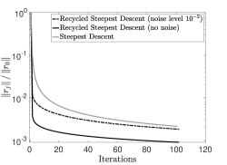
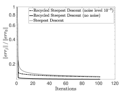
Figure 1: Residual and error convergence for large-scale Gaussian blur problem with $\sigma=6$ and augmentation space generated using vectors resulting from applying 2 iterations steepest descent to the noisy (dashed curve) and noise-free (solid black curve) data using Gaussian blur operators for five smaller standard deviations chosen equally-spaced from the interval $[0.5,1.5]$.

Our first experiment concerns an academic problem which serves as a proof of concept. However, we still execute a large-scale version of this experiment using an implicitly-defined, matrix free problem generated by the IR-Tools software package [17]. The IR-tools package does provide an out-of-the-box generator function for the Gaussian blurring problem, PRBlurGauss(); however, it does not allow one to specify precise standard deviation (i.e., the spread) of the point-spread function (PSF). Looking under the hood, though, one sees that there is a helper function called psfGauss() which generates a PSF function for a Gaussian with specified spread, which can then be fed into the general purpose PRBlur() problem generator, which outputs a matrix-free operator which convolves images with the PSF as well as the true solution and noisy right-hand side. A variety of solution images are available; we choose a predefined geometric pattern for this experiment. To make the problem sufficiently large-scale, we choose the image size to be $500\times 500$, meaning the implicit side of the matrix induced by the PSF is $250000\times 250000$. The IR-tools package is careful to not generate exact right-hand side data unless it is specified. We rerun PRBlur() with the option CommitCrime=‘true’ to obtain $\mathbf{b}_{true}$, but this is only used to understand the effects of noise in generating the recycling vectors. In these experiments, we generated the problem for standard deviation $\sigma=6$. To construct an augmentation subspace ${\mathcal{U}}$, we selected vectors resulting from applying two iterations of steepest descent to the right-hand side data but for different Gaussian blurring operators with five smaller standard deviations chosen equally-spaced from the interval $[0.5,1.5]$. An orthonormal basis for the span of these (nine) vectors was obtained and taken as ${\mathcal{U}}$. We also generated a set of “clean” recycled vectors using the noise-free $\mathbf{b}_{true}$, to see what effect noise has on the recycling process itself. It is demonstrated that such vectors do indeed offer better performance as recycled vectors, meaning that noise does effect the recycling process.

In Figure 1, we see that for both problems, this strategy yields an improvement in convergence, both for the noise-free and noise-contaminated problems. This is a promising numerical result and a proof of concept, but it requires further analysis and experimentation to understand it in the proper concept to guide the use of this strategy for real-world, non-academic problems.

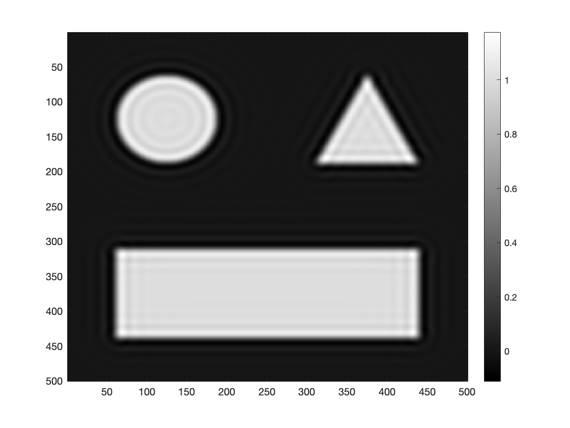
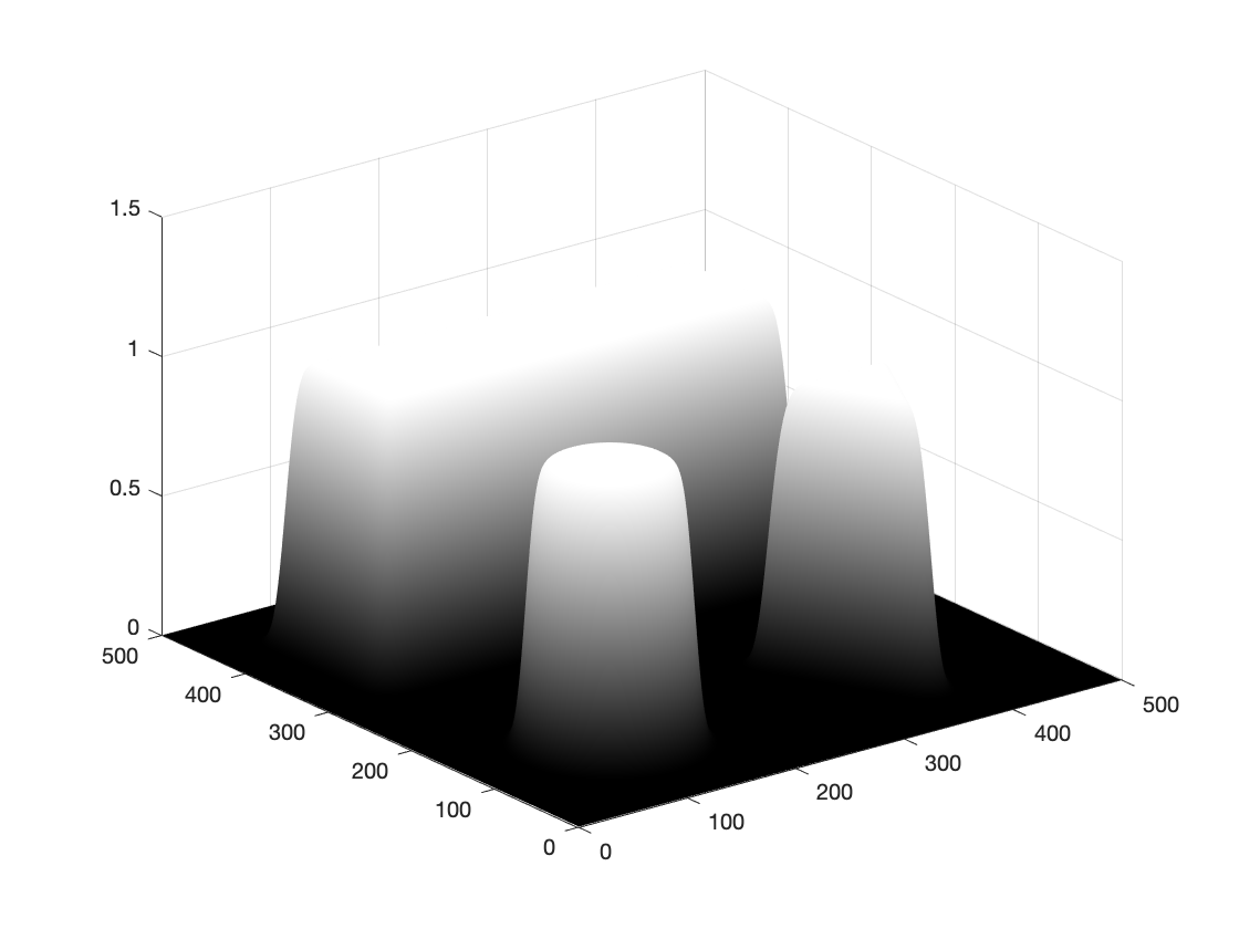
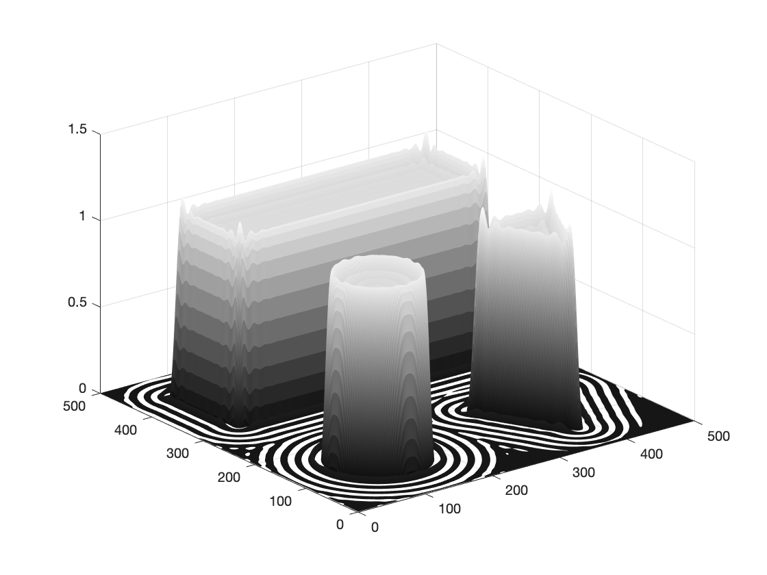
Figure 2: The right-hand side and the best reconstruction produced by steepest descent for each, respectively.

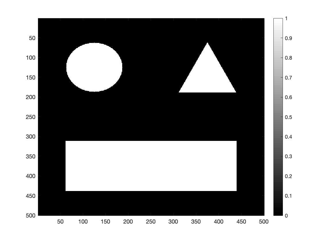
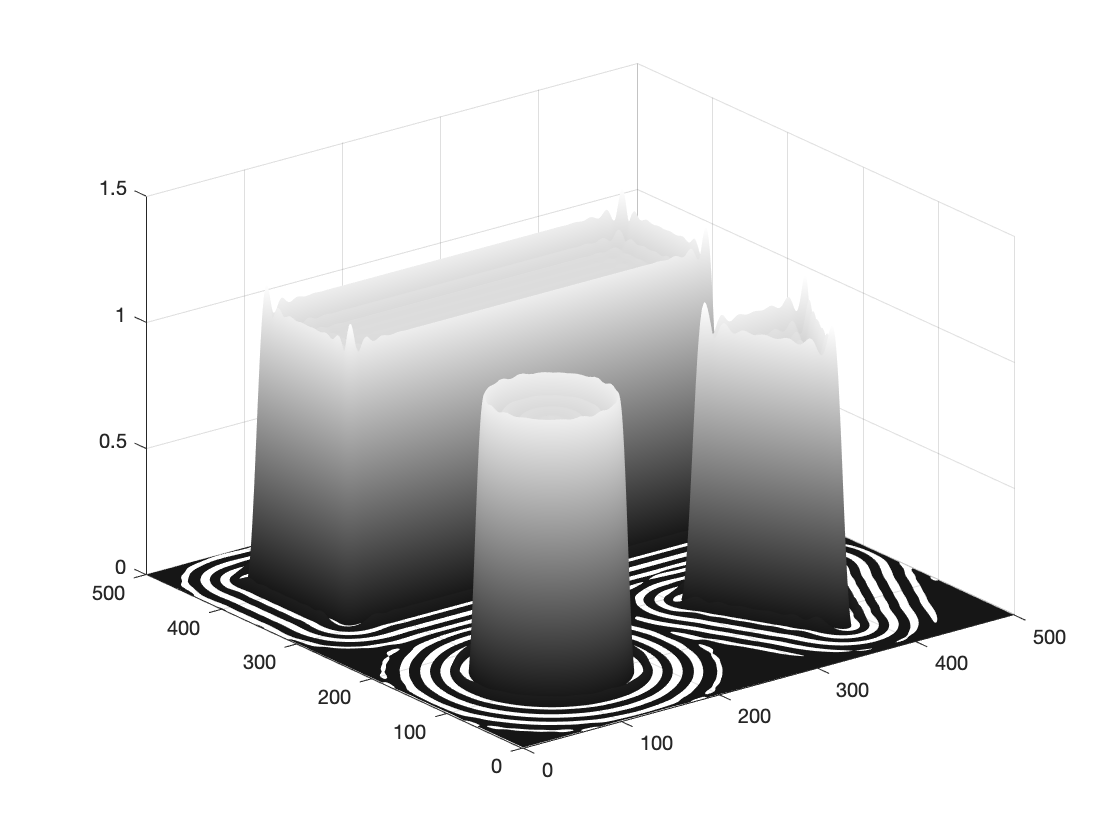
Figure 3: The true image and reconstructed images using augmented steepest descent We show them both as images in the top row and three-dimensional surfaces in the bottom row.

7.2 Adaptive optics: wavefront reconstruction

Turbulences in the atmosphere have a significant impact on the imaging quality of modern ground based telescopes. In order to correct for the impact of the atmosphere, Adaptive Optics (AO) systems are utilized. In these systems, the incoming light from bright guide stars is measured by wavefront sensors in order to obtain information of the actual turbulence in the atmosphere. In a next step, deformable mirrors use this information for an improvement of the obtained scientific images. For a review on the different mathematical aspects of AO systems we refer to [11]. E.g., Single Conjugate Adaptive Optics (SCAO) systems use one sensor and one mirror for the correction and are able to obtain a good image quality close to the direction of the guide star. Figure 4 shows a setup for a SCAO system. For the instruments of the new generation of telescopes, e.g., the Extremely Large Telescope (ELT) of the European Southern Observatory (ESO), the Pyramid sensor (P-WFS) will be used frequently to obtain the wavefront. A linear approximation of the connection between the incoming wavefront $\varphi$ and and the sensor measurements $(s_{x},s_{y})$ - assuming a non-modulated sensor - can be described as

(60) $$s_{x}(x,y)=\frac{1}{\pi}\int\limits_{-B(y)}^{B(y)}\frac{\Phi(x^{\prime},y)}{x-x^{\prime}}\,dx^{\prime}~{},$$

analogous for $s_{y}$. An overview of existing reconstruction methods for the P-WFS can be found in [22, 20, 19], and a throughout analysis of the various P-WFS models is given in [21, 21].

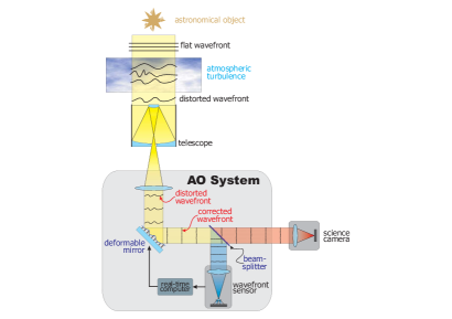
Figure 4: Principle of SCAO

The linear models can be used in case of small wavefront aberrations which is the case in a closed loop setting, i.e., if the wavefront sensor is optically located behind the deformable mirror. Due to the rapidly changing atmosphere, the shape of the deformable mirror has to be readjusted every 1-2 milliseconds over the whole imaging process, which might last several minutes. Therefore, the reconstructions of the wavefronts have to be accurate and have to be obtained in real-time. As a quality measure we use the Strehl ratio ($SR$), which relates the imaging quality of the telescope without disturbing atmosphere ($SR=1$) to the corrected imaging quality, i.e.. $SR\in[0,1]$. In the beginning of the observation the Strehl ratio is low, as the deformable mirror is not yet adjusted to the turbulence conditions. After a few time steps, the mirror is in a state where only small adjustments are necessary - the loop has been closed. This happens in our case when $SR\in[0.6,0.7]$. In this state, the linear modes for the P-WFS are valid. We show the utility of the recycled steepest descent method for multiple steps of an closed-loop iteration for a wavefront reconstruction for the instrument METIS of the ELT. The recycling subspaces were formed by the previous $1-3$ reconstructions, see Fig. 5 for the results. In the long run, both steepest descent with recycling and warm restart (i.e, where the last reconstruction is used as a starting value for the new reconstruction) yield the same Strehl ratio. However, the method with recycling is able to close the loop much faster, which is important for a stable and efficient imaging of the scientific object.

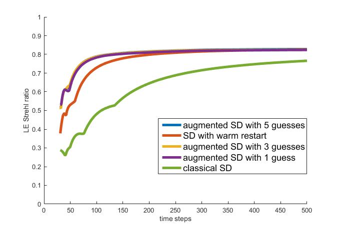
Figure 5: Monitoring of wavefront reconstruction accuracy over time.

7.3 Adaptive optics: Image reconstruction

Our final example concerns another problem related to astronomical imaging. As for any optical system, the design of the system determines the obtainable imaging quality: Instead of the ”true” image one always obtains a blurred image. The extend of blurring is described mathematically by the point spread function (PSF) of the optical system, and the measured image can be modeled as the convolution of the true image and the PSF:

(61) $$I(t)=\int I_{true}(s)\cdot PSF(t-s)\,ds.$$

Thus, the original image can be recovered - assuming the PSF is known - by solving the linear ill-posed problem (61). In this example we want to reconstruct an astronomical image from the measured image obtained by a telescope using the approximate PSF of the telescope. It is well known that the PSF of a telescope without a turbulent atmosphere above the telescope (e.g., a telescope in space) is given by

(62) $$PSF_{\color[rgb]{0,0,0}0}(x)=\left|{\mathcal{F}}\{P\}(x)\right|^{2}$$

where $P$ is the characteristic function of the aperture of the main mirror of the telescope (usually an annulus) and ${\mathcal{F}}(\cdot)$ represents the Fourier transform of the argument. Please note that the recovery of the original image from the measured one results in most cases in an ill posed problem, at least for smooth PSF, which is, e.g., the case for (62). For ground based telescopes, however, the turbulent atmosphere above the telescope has to be taken into account. The related PSF can be modeled as

(63) $$PSF_{\phi}(x,t)=\left|{\mathcal{F}}\{P(\cdot)e^{i\phi(\cdot,t)}\}(x)\right|^{2}.$$

Here, $\phi(r,t)$ describes the turbulence above the telescope. As we have seen above, an AO systems aims to reduce the impact of the turbulence to the imaging process - see Section 7.2. For various reasons, e.g., the time delay between measuring the turbulences and their correction or the limited resolution of wavefront sensors and deformable mirrors, such an correction will never be perfect and therefore there will always remain a residual (uncorrected) turbulence. Based on the data from the AO system it is, however, possible to estimate those uncorrected turbulences and obtain an approximation of $PSF_{\phi}$ of the observation. A full description of this problem, i.e. the reconstruction of the PSF from AO data of the scientific observation, can be found, e.g., in [10, Section 5.4] and references therein. As astronomical images are acquired over a period of time, one actually recovers a time-averaged PSF, denoted $\left\langle PSF_{\phi}(\cdot,t)\right\rangle$.
In our experiments, the time averaged $PSF_{\phi}$ with residual turbulences taken into account is simulated by OCTOPUS [26, 25], the simulation tool of the European Southern Observatory. In addition, we use a representation of $PSF(x)$, the PSF of the telescope without turbulences. Both PSFs are represented by matrices, i.e., as the functions spatially discretized for images of a certain size. Please note that the recovery of the original image from the convolution data remains ill-posed in both cases.

Convolution of images with PSFs was performed using the function psfMatrix() available, .e.g., as a part of the Matlab toolbox IRTools [17]. We use the Star Cluster image, which can be obtained from the test problems of the Matlab package Restore Tools [1]. The provided artificial Star Cluster image is $257\times 257$; so for these experiments, the discretized PSFs are resized (i.e., downscaled) to also be $257\times 257$ using the imresize() function of Matlab. A psfMatrix object is then instantiated which can be applied via multiplication to an image to perform a convolution, i.e.,

$$\tt Apsf=psfMatrix(psf\_257,`periodic^{\prime},[C\ C],[N\ N])$$

where $N=257$ and $C=129$, the center coordinate of the image, and we use periodic boundary conditions. Entry $(C,C)$ of the PSF indicates where the value of the PSF at $(0,0)$ is located, where we assume the square image is centered at the origin. The PSF inducing the adjoint operator can be created via the relation $PSFadj(x,y)=PSF(-x,-y)$ which, along with the image being centered at the origin, can be used to construct the discrete PSF inducing the discretized adjoint operator [39]. In Figure 6, we show log plots of the true Star Cluster image and its blurred counterpart convolved with the PSF representing the atmospheric distortion. The blurred image was perturbed with random noise generated with uniform distribution using Matlab’s rand() function, which was then scaled to have norm $10^{-1}\left\|b\right\|_{F}$, where $b$ represents the convolved true image shown on the right in Figure 6.

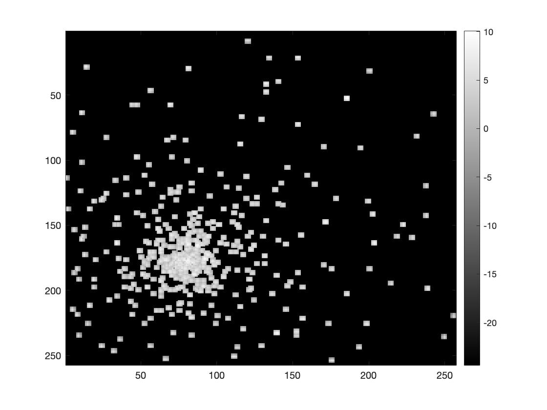
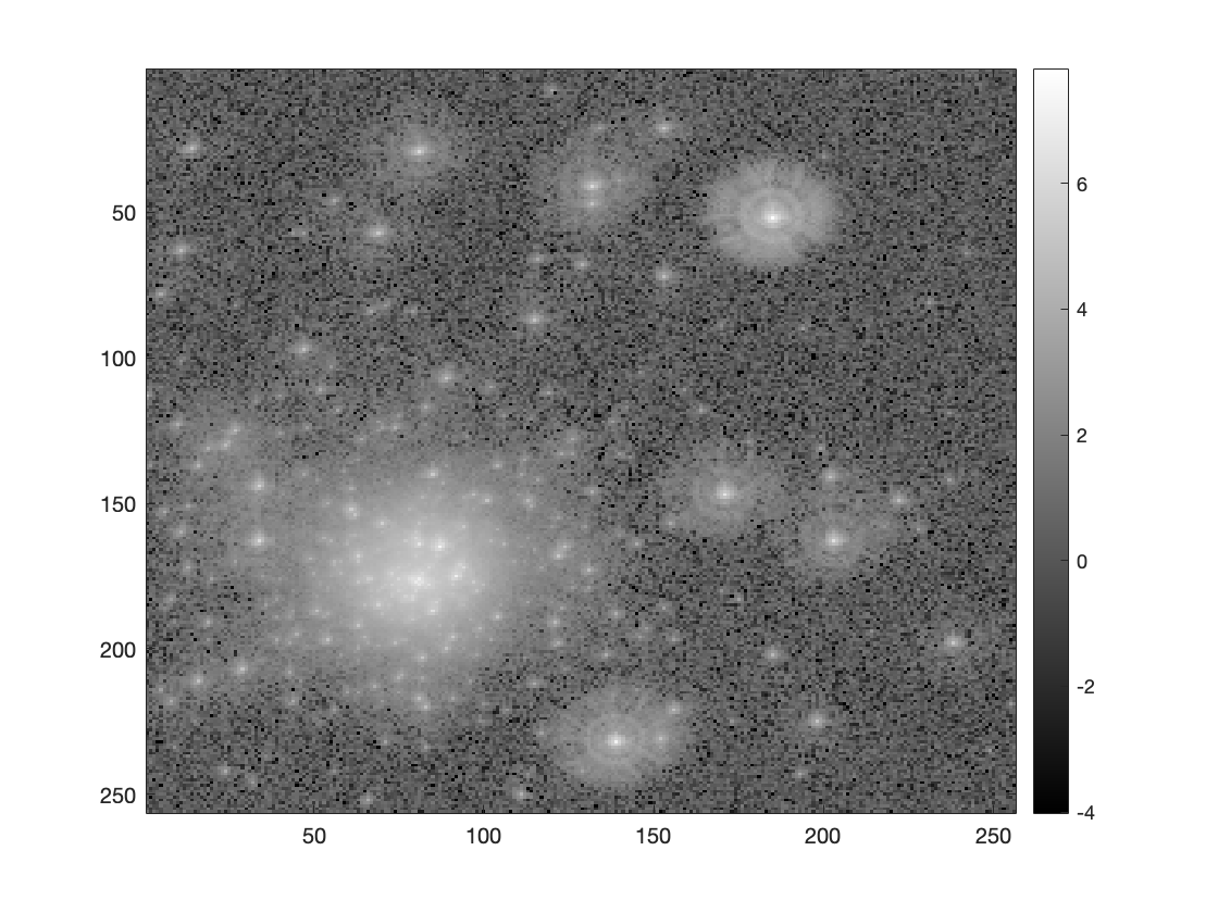
Figure 6: The true and blurred Star Cluster image with generated stars of various brightnesses, with the true image shown in log-plot to clearly show all the generated stars clearly

In this study, we demonstrate that subspace recycling works well for the considered deconvolution problem. As for a telescope with a good AO system $PSF_{0}$ is at least a coarse approximation of $PSF_{\phi}$, we propose to form the recycling subspace from a few eigenvectors of the matrix representing $PSF_{0}$. Here, we take advantage of the fact that although $PSF_{\phi}$ changes for every observation, $PSF_{0}$ remains constant. This enables us to pre-calculate eigenvectors of its induced convolution operator ahead of time offline.

We calculated the telescope eigenvectors via the matrix-free eigs() routine of Matlab which uses a Krylov-based iteration to compute eigenvalues and eigenvectors for a few of the largest eigenvalues of the operator. In this experiment, we chose to compute the top 200 but had to perform post-processing step to eliminate the spurious complex eigenvalues/-vectors that are created in pairs, leaving us with 198 eigenvalues. Ordering the eigenvalues thereof in descending order, we augment with different collections of these pre-computed eigenvectors, starting with just the first, then the first two, and so on, up to all 198. In Figure 7, we show the residual and error curves for all experiments together. One sees that augmenting with these eigenvectors is effective in increasing the speed of convergence of the steepest descent method, with acceleration increasing as we add more vectors, but with diminishing returns.

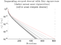
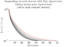
Figure 7: Residual and error convergence of steepest descent (shown in red) and augmented steepest descent (shown in shades of gray) with augmentation spaces being eigenvectors of the operator induced by the telescope PSF, where we used the eigenvectors associated to the largest eigenvalues. The curve’s darkness is determined by how many eigenvectors were used in the augmentation. More vectors produces a darker curve.

It is important to investigate how long it takes to achieve some manner of semiconvergence. Thus, for each experiment, we track at which iteration semiconvergence is achieved and also at which iteration the residual-based discrepancy principle is achieved. For the operator induced by the telescope PSF, we also monitor jumps in eigenvalue magnitude, and these are plotted separately. This is shown in Figure 8. We also show for completeness the first nine eigenvectors (i.e., eigenimages) of the operator induced by the telescope PSF in Figure 9.

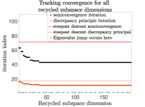
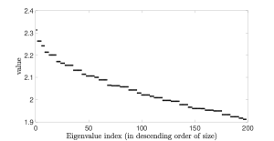
Figure 8: We show (left figure) for each recycled subspace dimension from this experiment at what iteration semiconvergence and the discrepancy principle are achieved, and we also mark where jumps in the eigenvalues of the operator induced by the PSF (the Airy function) of the telescope occur. On the right, we show the eigenvalues of this operator.

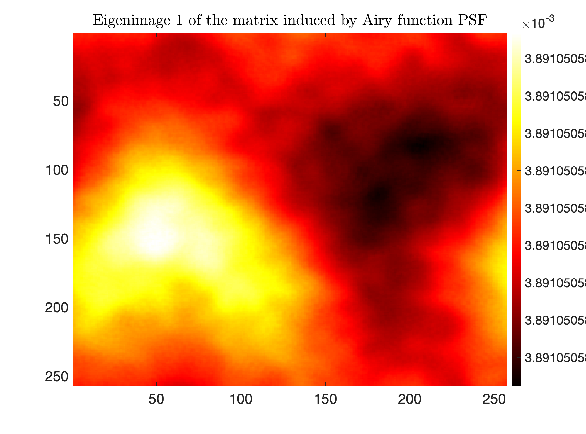
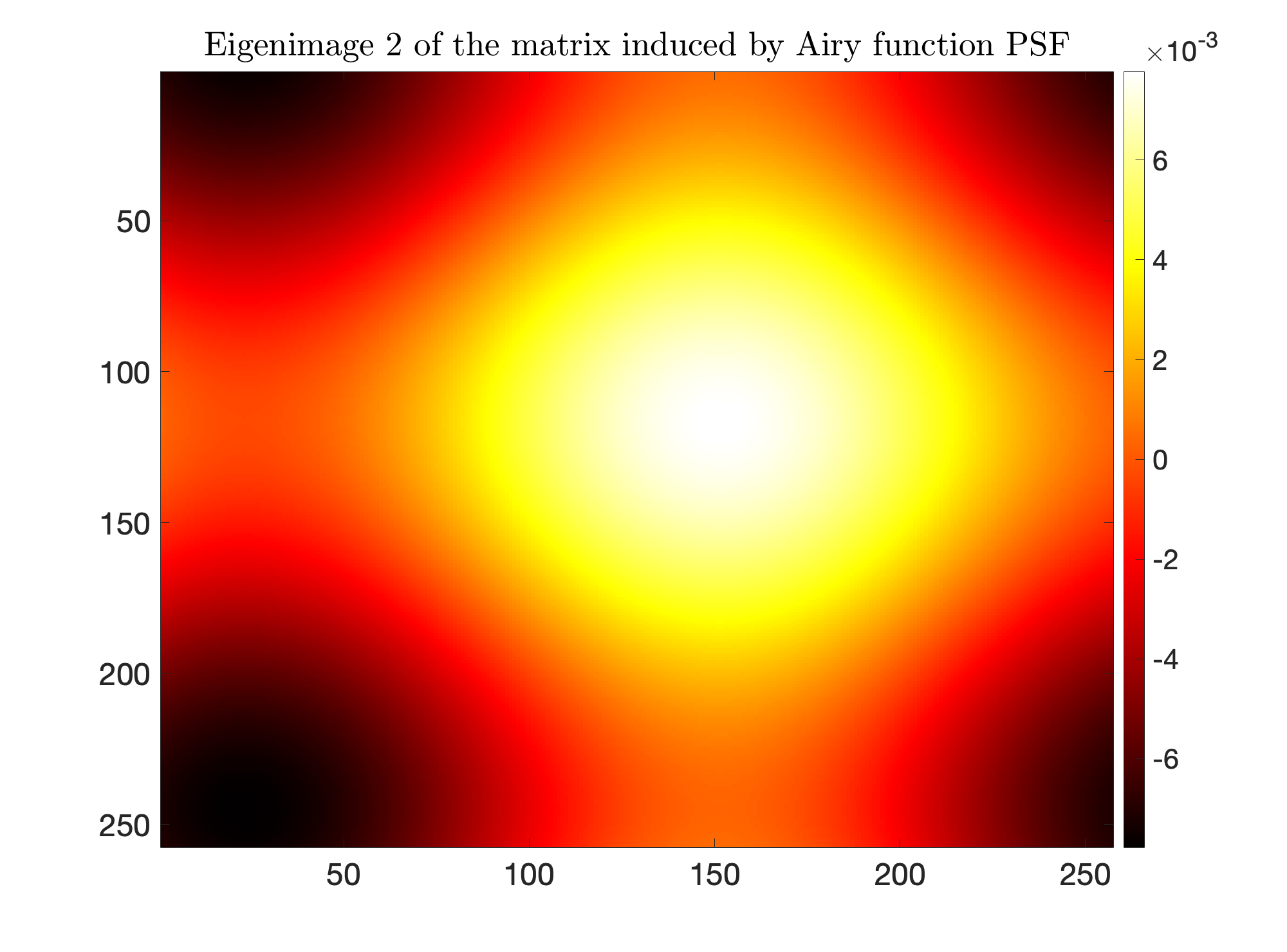
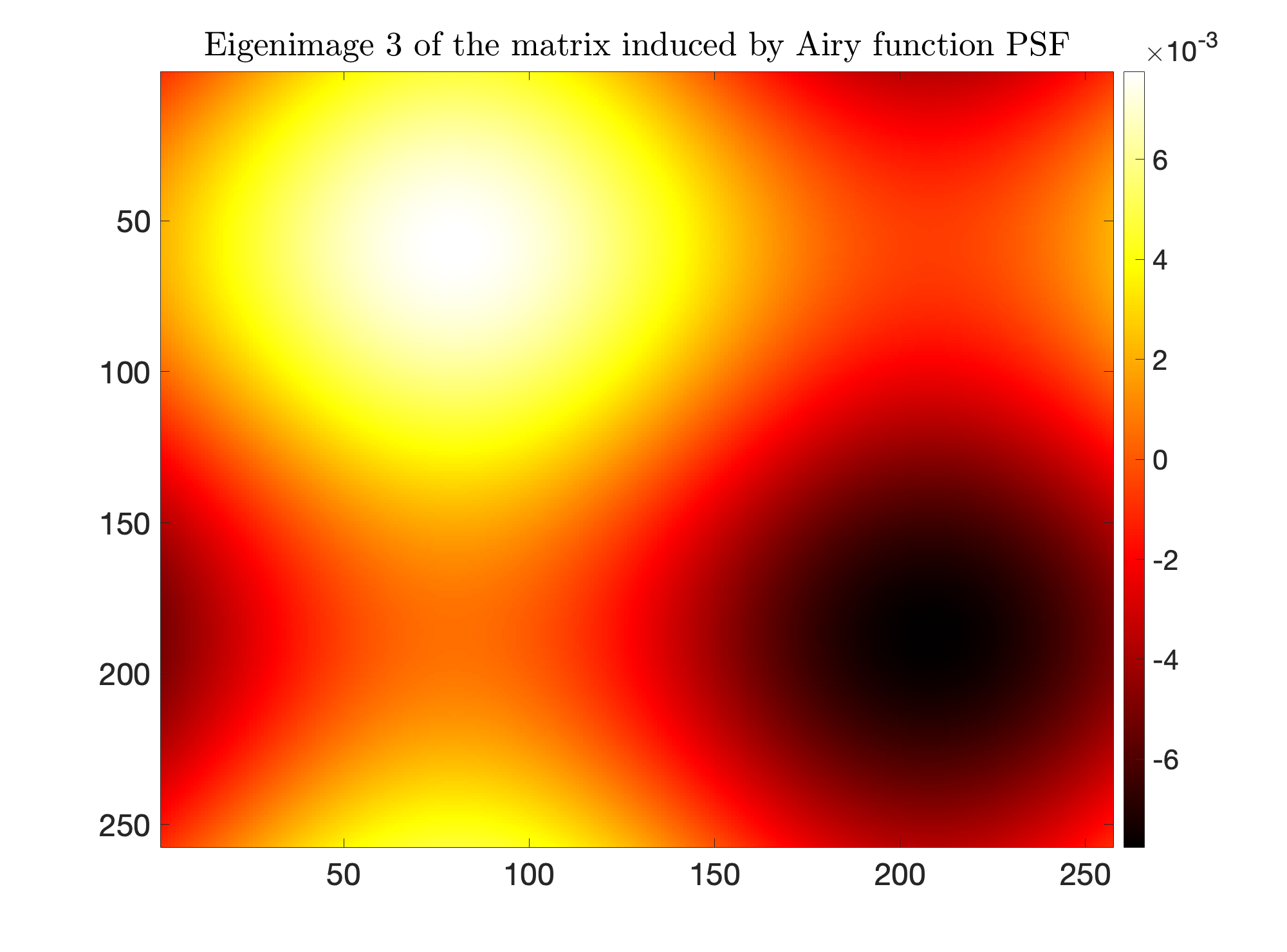
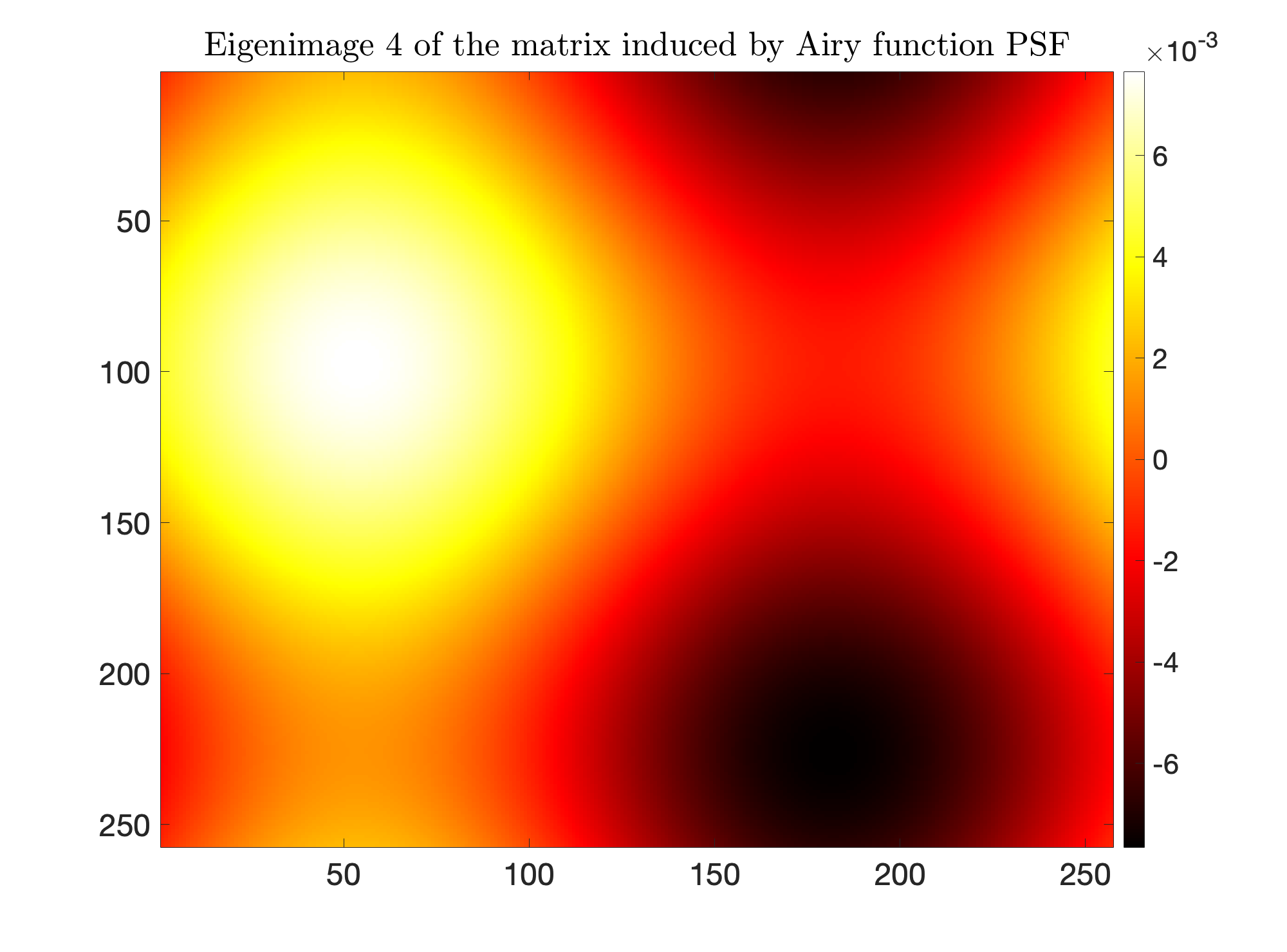
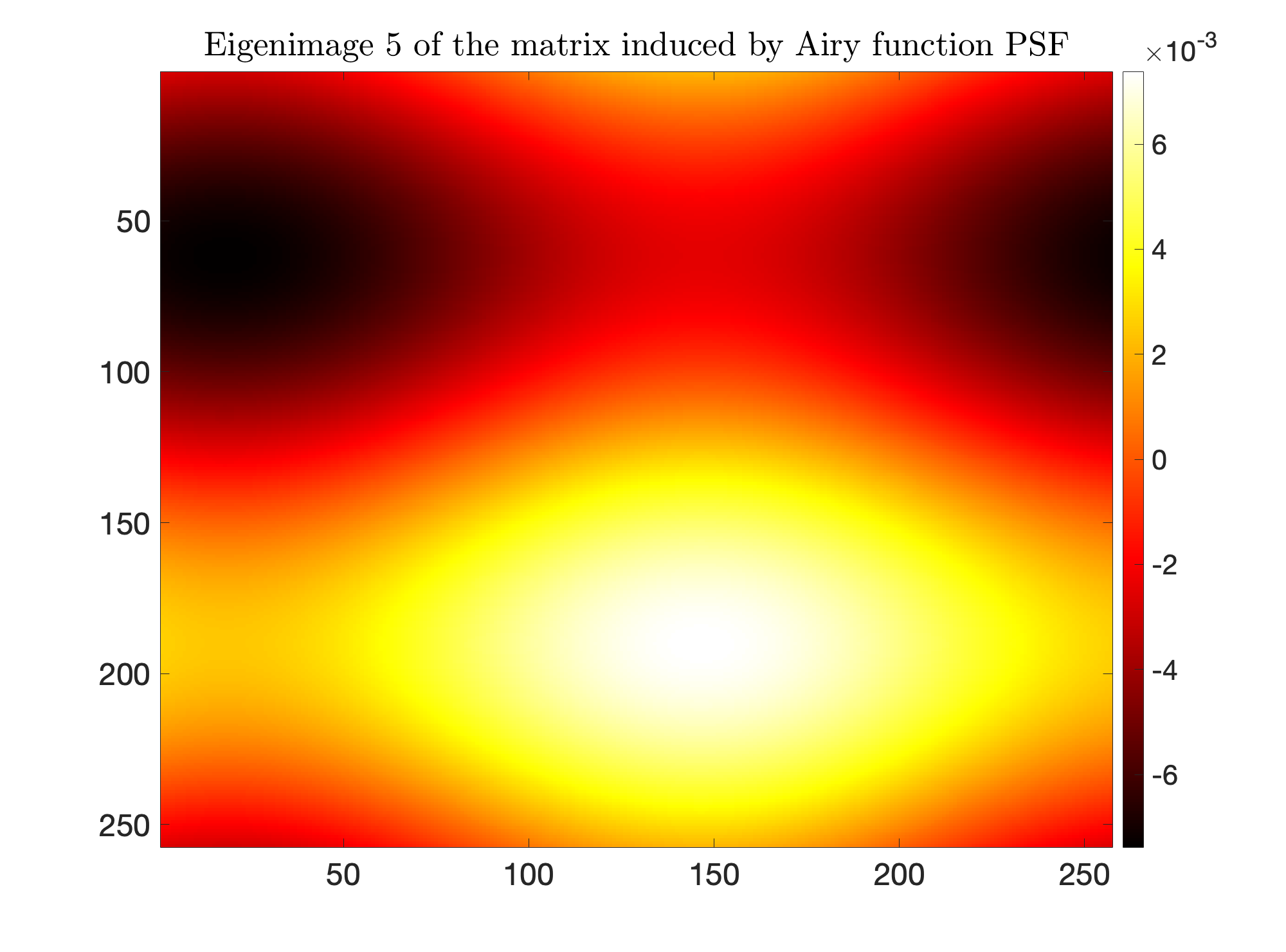
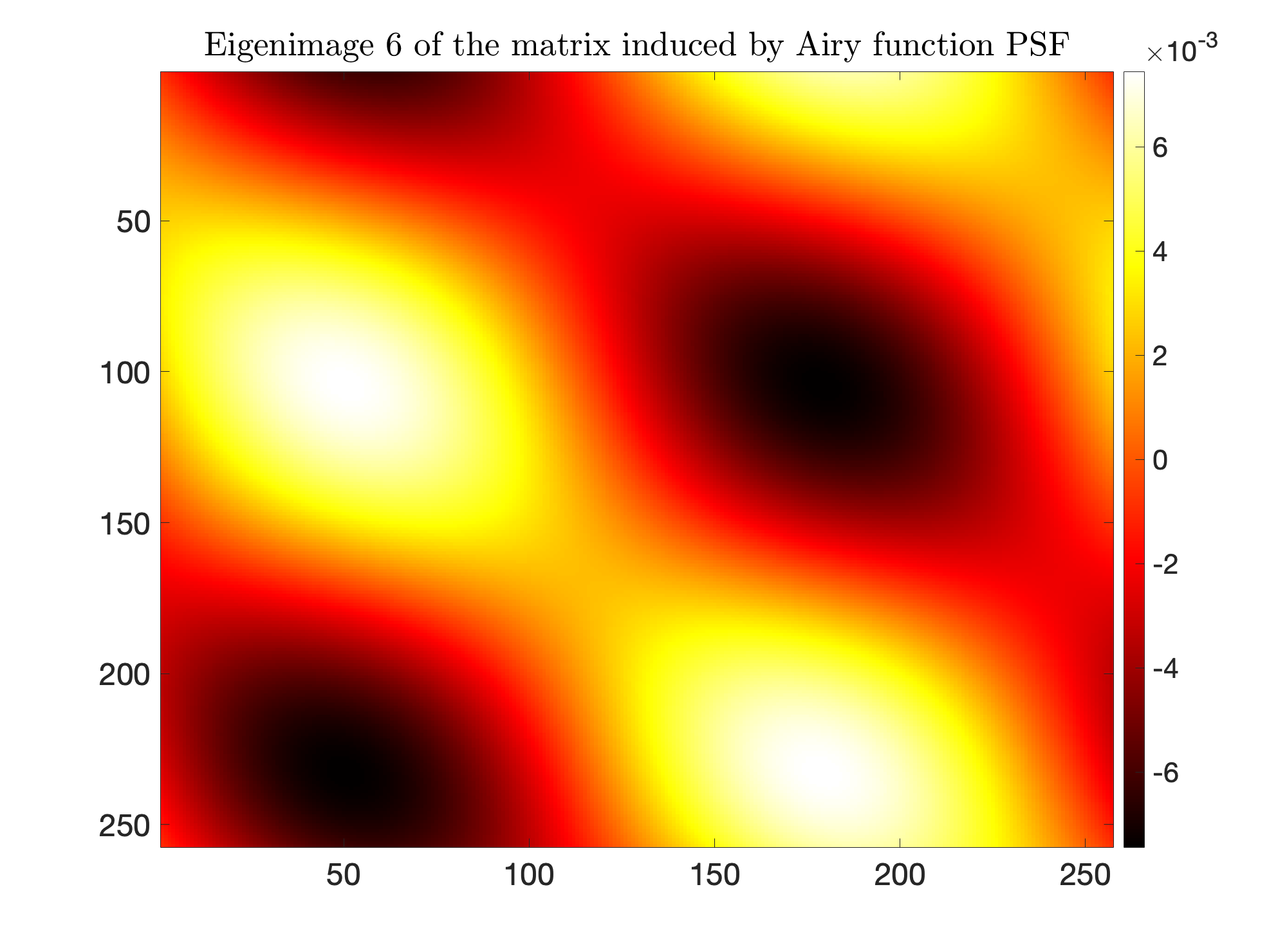
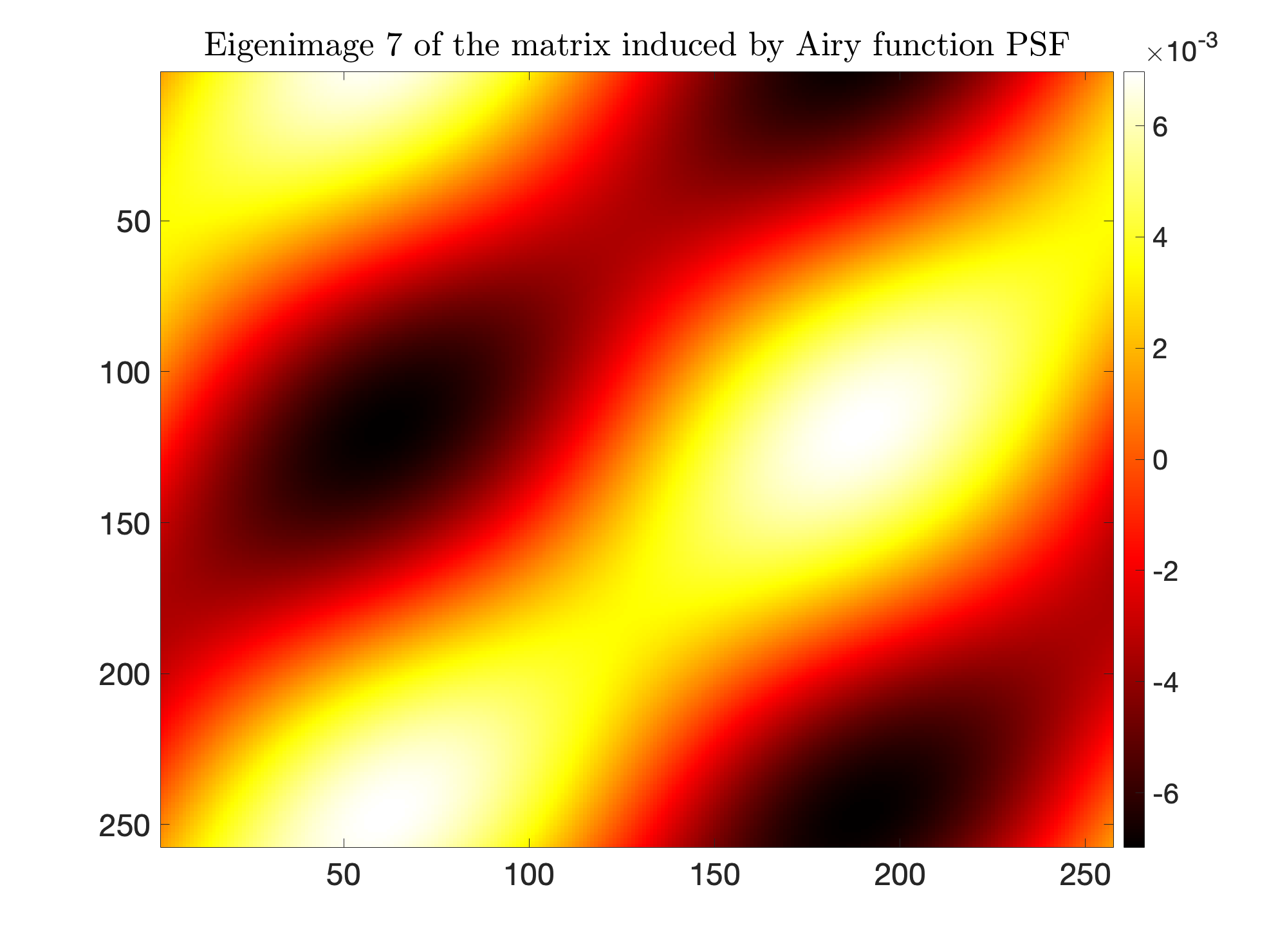
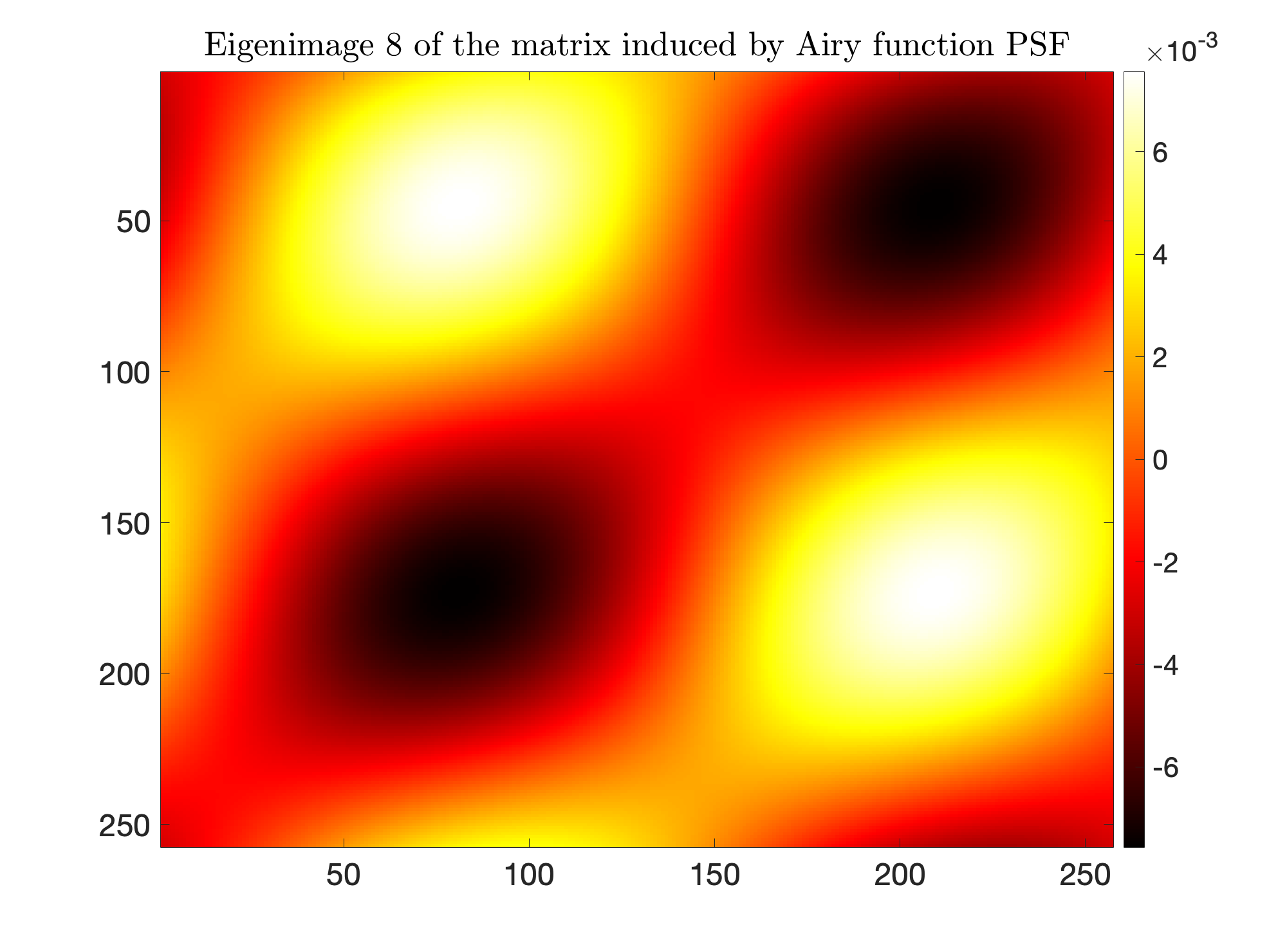
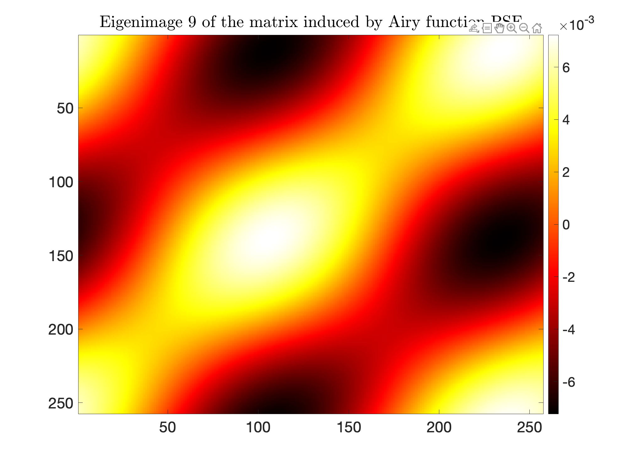
Figure 9: The first nine eigenfuntions (with eigenvalues in descending order) of the operator induced by the PSF, i.e., Eq. 63, of the telescope. Note that the first function is actually a constant up to roundoff noise.

Lastly, for the case in which we augmented with the first 37 eigenvectors, we show the actual image produced at the iteration in which semiconvergence was reached. We show both the raw image produced by augmented steepest descent, as well as one post-processed by thresholding pixels with values less than $10$ to be zero. This is shown (again in log plot) in Figure 10. Augmentation of additional eigenvectors beyond the first 37 produced no additional improvement for this problem.

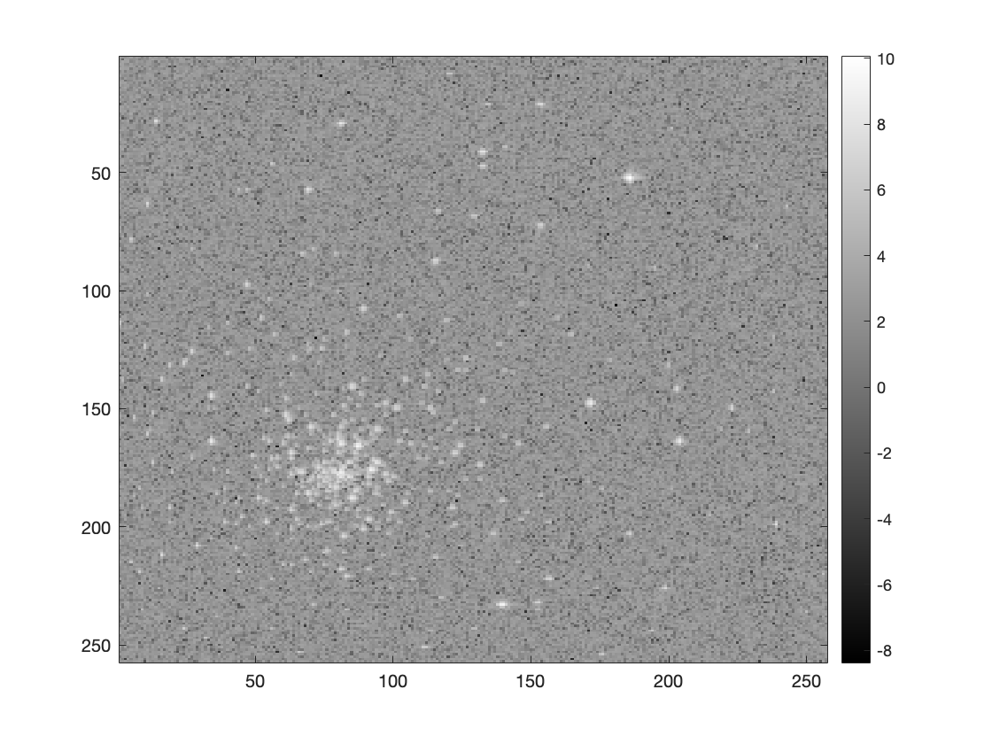
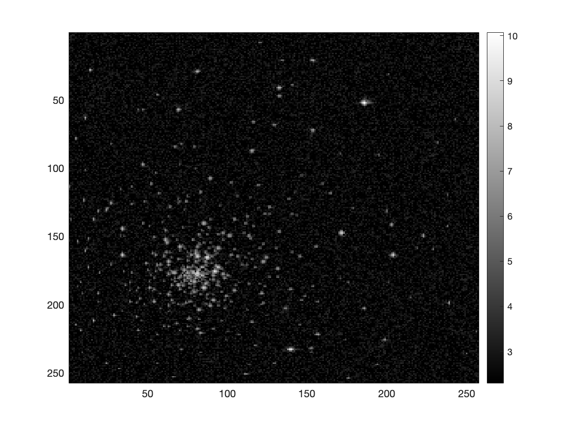
Figure 10: The image produced by augmented steepest descent at the semiconvergence iteration, raw and with pixel thresholding (all pixels of value less than $10$ thresholded to zero), for the experiment augmenting the first 37 eigenvectors.

8 Conclusions

In this paper, we have shown that under basic assumptions, the subspace recycling scheme can be combined with any known regularization scheme, and the resulting augmented scheme is still a regularization. This opens many possibilities for schemes for developing new augmented regularization schemes. We have further demonstrated this by proposing an augmented gradient descent scheme, and we show how useful recycling easily-computed information within the augmented gradient descent method can be for accelerating semi-convergence, both in an academic problem and in problems arising from applications in astronomy.

References

• [1] Restoretools: An object oriented matlab package for image restoration, 2012, http://www.mathcs.emory.edu/~nagy/RestoreTools/. Accessed on 28. June 2020.
• [2] K. Ahuja, E. de Sturler, S. Gugercin, and E. R. Chang, Recycling BiCG with an application to model reduction, SIAM J. Sci. Comput., 34 (2012), pp. A1925–A1949, https://doi.org/10.1137/100801500, http://dx.doi.org/10.1137/100801500.
• [3] J. Baglama and L. Reichel, Augmented GMRES-type methods, Numerical Linear Algebra with Applications, 14 (2007), pp. 337–350, https://doi.org/10.1002/nla.518, http://dx.doi.org/10.1002/nla.518.
• [4] J. Baglama and L. Reichel, Decomposition methods for large linear discrete ill-posed problems, Journal of Computational and Applied Mathematics, 198 (2007), pp. 332–343, https://doi.org/10.1016/j.cam.2005.09.025, http://dx.doi.org/10.1016/j.cam.2005.09.025.
• [5] J. Chung, E. de Sturler, and J. Jiang, Hybrid projection methods with recycling for inverse problems, (2020), https://arxiv.org/abs/2007.00207.
• [6] E. de Sturler, Nested Krylov methods based on GCR, Journal of Computational and Applied Mathematics, 67 (1996), pp. 15–41, https://doi.org/10.1016/0377-0427(94)00123-5, http://dx.doi.org/10.1016/0377-0427(94)00123-5.
• [7] E. de Sturler, M. Kilmer, and K. M. Soodhalter, Krylov subspace augmentation for the solution of shifte systems: a review. in preparation.
• [8] M. Defrise and C. D. Mol, A note on stopping rules for iterative methods and filtered svd, in Inverse Problems: An Interdisciplinary Study, P. C. Sabatier, ed., Academic Press, 1987, pp. 261–268.
• [9] Y. Dong, H. Garde, and P. C. Hansen, R3GMRES: including prior information in GMRES-type methods for discrete inverse problems, Electron. Trans. Numer. Anal., 42 (2014), pp. 136–146.
• [10] L. Dykes, R. Ramlau, L. Reichel, K. M. Soodhalter, and R. Wagner, Lanczos-based fast blind deconvolution methods, Journal of Computational and Applied Mathematics, (To Appear).
• [11] B. Ellerbroek and C. Vogel, Inverse problems in astronomical adaptive optics, Inverse Problems, 25 (2009), p. 063001.
• [12] H. Engl and R. Ramlau, Regularization of Inverse Problems, Springer, New York, 2015, pp. 1233–1241.
• [13] H. W. Engl, M. Hanke, and A. Neubauer, Regularization of inverse problems., Dordrecht: Kluwer Academic Publishers, 1996.
• [14] Y. A. Erlangga and R. Nabben, Deflation and balancing preconditioners for Krylov subspace methods applied to nonsymmetric matrices, SIAM Journal on Matrix Analysis and Applications, 30 (2008), pp. 684–699.
• [15] A. Gaul, Recycling Krylov subspace methods for sequences of linear systems: Analysis and applications, PhD thesis, Technischen Universität Berlin, 2014.
• [16] A. Gaul, M. H. Gutknecht, J. Liesen, and R. Nabben, A framework for deflated and augmented Krylov subspace methods, SIAM Journal on Matrix Analysis and Applications, 34 (2013), pp. 495–518, https://doi.org/10.1137/110820713, http://dx.doi.org/10.1137/110820713.
• [17] S. Gazzola, P. C. Hansen, and J. G. Nagy, IR Tools: a MATLAB package of iterative regularization methods and large-scale test problems, Numer. Algorithms, 81 (2019), pp. 773–811, https://doi.org/10.1007/s11075-018-0570-7, https://doi-org.libproxy.temple.edu/10.1007/s11075-018-0570-7.
• [18] M. H. Gutknecht, Deflated and augmented Krylov subspace methods: a framework for deflated BiCG and related solvers, SIAM J. Matrix Anal. Appl., 35 (2014), pp. 1444–1466, https://doi.org/10.1137/130923087, https://doi-org.libproxy.temple.edu/10.1137/130923087.
• [19] V. Hutterer and R. Ramlau, Nonlinear wavefront reconstruction methods for pyramid sensors using Landweber and Landweber-Kaczmarz iteration, Applied Optics, 57 (2018), pp. 8790–8804.
• [20] V. Hutterer and R. Ramlau, Wavefront reconstruction from non-modulated pyramid wavefront sensor data using a singular value type expansion, Inverse Problems, 34 (2018), p. 035002.
• [21] V. Hutterer, R. Ramlau, and I. Shatokhina, Real-time adaptive optics with pyramid wavefront sensors: part I. a theoretical analysis of the pyramid sensor model, Inverse Problems, 35 (2019), p. 045007, https://doi.org/10.1088/1361-6420/ab0656, https://doi.org/10.1088%2F1361-6420%2Fab0656.
• [22] R. R. I. Shatokhina, V. Hutterer, Review on methods for wavefront reconstruction from pyramid wavefront sensor data, Journal of Astronomical Telescopes, Instruments and Systems, 6 (2020), p. 010901, https://doi.org/10.1117/1.JATIS.6.1.010901.
• [23] M. E. Kilmer and E. de Sturler, Recycling subspace information for diffuse optical tomography, SIAM Journal on Scientific Computing, 27 (2006), pp. 2140–2166, https://doi.org/10.1137/040610271, http://dx.doi.org/10.1137/040610271.
• [24] L. Landweber, An Iteration Formula for Fredholm Integral Equations of the First Kind, American Journal of Mathematics, 73 (1951), pp. 615–624.
• [25] M. Le Louarn, C. Vérinaud, V. Korkiakoski, and E. Fedrigo, Parallel simulation tools for AO on ELTs, in Advancements in Adaptive Optics, Proc. SPIE 5490, 2004, pp. 705–712.
• [26] M. Le Louarn, C. Vérinaud, V. Korkiakoski, N. Hubin, and E. Marchetti, Adaptive optics simulations for the European Extremely Large Telescope - art. no. 627234, in Advances in Adaptive Optics II, Prs 1-3, vol. 6272, 2006, pp. U1048–U1056.
• [27] A. K. Louis, Inverse und schlecht gestellte Probleme, Teubner Studienbücher Mathematik, Vieweg+Teubner Verlag, 1989.
• [28] R. B. Morgan, GMRES with deflated restarting, SIAM J. Sci. Comput., 24 (2002), pp. 20–37, https://doi.org/10.1137/S1064827599364659, https://doi-org.libproxy.temple.edu/10.1137/S1064827599364659.
• [29] M. L. Parks, E. de Sturler, G. Mackey, D. D. Johnson, and S. Maiti, Recycling Krylov subspaces for sequences of linear systems, SIAM Journal on Scientific Computing, 28 (2006), pp. 1651–1674, https://doi.org/10.1137/040607277, http://dx.doi.ofrrg/10.1137/040607277.
• [30] M. L. Parks, K. M. Soodhalter, and D. B. Szyld, A block recycled gmres method with investigations into aspects of solver performance, (2016), https://arxiv.org/abs/1604.01713.
• [31] R. Ramlau and M. Rosensteiner, An efficient solution to the atmospheric turbulence tomography problem using Kaczmarz iteration, Inverse Problems, 28 (2012), p. 095004.
• [32] R. Ramlau and B. Stadler, An augmented wavelet reconstructor for atmospheric tomography, 2020, https://arxiv.org/abs/2011.06842.
• [33] Y. Saad, Krylov subspace methods for solving large unsymmetric linear systems, Mathematics of Computation, 37 (1981), pp. 105–126, https://doi.org/10.2307/2007504, http://dx.doi.org/10.2307/2007504.
• [34] Y. Saad, Iterative Methods for Sparse Linear Systems, SIAM, Philadelphia, Second ed., 2003.
• [35] O. Scherzer, M. Grasmair, H. Grossauer, M. Haltmeier, and F. Lenzen, Variational Methods in Imaging, Springer, New York, 2009.
• [36] K. M. Soodhalter, E. de Sturler, and M. Kilmer, A survey of subspace recycling iterative methods, GAMM Mitteilungen, (2020). Applied and numerical linear algebra topical issue.
• [37] L. N. Trefethen and D. Bau, III, Numerical linear algebra, Society for Industrial and Applied Mathematics (SIAM), Philadelphia, PA, 1997, https://doi.org/10.1137/1.9780898719574, https://doi-org.libproxy.temple.edu/10.1137/1.9780898719574.
• [38] S. Wang, E. de Sturler, and G. H. Paulino, Large-scale topology optimization using preconditioned Krylov subspace methods with recycling, International Journal for Numerical Methods in Engineering, 69 (2007), pp. 2441–2468, https://doi.org/10.1002/nme.1798, http://dx.doi.org/10.1002/nme.1798.
• [39] R. Wanger. Personal Communication, Mar. 2020.
• [40] M. Yudytskiy, T. Helin, and R. Ramlau, Finite element-wavelet hybrid algorithm for atmospheric tomography, J. Opt. Soc. Am. A, 31 (2014), pp. 550–560, https://doi.org/10.1364/JOSAA.31.000550, http://josaa.osa.org/abstract.cfm?URI=josaa-31-3-550.