Lattice Meets Lattice:
Application of Lattice Cubature to
Models in Lattice Gauge Theory

Abstract

High dimensional integrals are abundant in many fields of research including quantum physics. The aim of this paper is to develop efficient recursive strategies to tackle a class of high dimensional integrals having a special product structure with low order couplings, motivated by models in lattice gauge theory from quantum field theory. A novel element of this work is the potential benefit in using lattice cubature rules. The group structure within lattice rules combined with the special structure in the physics integrands may allow efficient computations based on Fast Fourier Transforms. Applications to the quantum mechanical rotor and compact $\mathit{U}(1)$ lattice gauge theory in two and three dimensions are considered.

1 Introduction

High dimensional integrals are abundant in many fields of research including quantum physics. The aim of this paper is to develop efficient recursive strategies to tackle a class of high dimensional integrals having a special product structure with low order couplings, motivated by models in lattice gauge theory [15] from quantum field theory. A novel element of this work is the potential benefit in using lattice cubature rules [13, 29]. The group structure within lattice rules combined with the special structure in the physics integrands may allow efficient computations based on Fast Fourier Transforms (FFT). Note the two different occurrences of the word “lattice” here: one as a discretization tool in physics, and one as a method of approximating integrals in numerical analysis.

The integrals being considered are motivated by problems from simulations of quantum field theories, e.g., systems in high energy and statistical physics. In the simplest formulation, we have an $L$-dimensional integral of the form

$$\int_{D^{L}}\prod_{i=0}^{L-1}f_{i}\big{(}x_{i},x_{i+1}\big{)}\,\mathrm{d}\boldsymbol{x},\qquad\mbox{with $\boldsymbol{x}=(x_{0},\ldots,x_{L-1})$ and $x_{L}\equiv x_{0}$,}$$ (1)

where each variable $x_{i}$ belongs to a bounded domain $D\subset{\mathbb{R}}$ and each function $f_{i}$ depends only on two consecutive variables $x_{i}$ and $x_{i+1}$. We will refer to the condition $x_{L}\equiv x_{0}$ as “parametric periodicity”. This is a defining characteristic of the class of problems that we consider in this paper. Models in lattice field theory often couple the relevant degrees of freedom on neighboring lattice sites, and as a result exhibit the structure of (1). As a concrete example we consider here the topological oscillator or quantum rotor, see [1, 7, 8] and Section 2.1 below, which is a 1D (i.e., one space-time dimension) quantum mechanical model in Euclidean time with $L$ lattice points. Often the functions $f_{i}$ are identical (or only one of them is different due to the presence of the “observable function”), depend only on the difference of the two input variables, and are periodic in each coordinate direction. For example, $f_{i}(u,v)=\exp(\beta\cos(v-u))$ with $D=[-\pi,\pi)$.

Note that there are two senses of dimensionality here: typically by dimension we are referring to the number of integration variables, denoted by $L$ in (1) and later more generally denoted by $s$; but there is also the space-time dimension of the underlying physical problem which we will denote by $d$ and describe as 1D, 2D or 3D (i.e., $d=1,2,3,\ldots$).

Often in high energy and statistical physics, integrals of the form (1) appear in both the numerator and denominator of a ratio that represents the expected value of an observable (see e.g., (8) below). The end goal is typically to obtain this ratio rather than the separate integrals, and a popular strategy is to tackle this using Markov chain Monte Carlo $($MCMC$)$ simulations. Here instead we propose to treat the integrals by numerical integration methods.

One possibility is to apply an $L$-fold tensor product of a one-dimensional quadrature rule to approximate the integral (1). That is, each integral over $D$ in (1) is approximated by a one-dimensional quadrature rule with $n$ points $t_{1},\ldots,t_{n}\in D$ and corresponding weights $w_{1},\ldots,w_{n}\in{\mathbb{R}}$, so that the approximation to (1) is given by

$$\sum_{k_{0}=0}^{n-1}w_{k_{0}}\cdots\sum_{k_{L-1}=0}^{n-1}w_{k_{L-1}}\,\prod_{i=0}^{L-1}f_{i}\big{(}t_{k_{i}},t_{k_{i+1}}\big{)},$$ (2)

where for convenience we extend parametric periodicity to the notation of indices so that $k_{L}\equiv k_{0}$.

We switch now to the general notation with $s$ instead of $L$ denoting the number of integration variables. The approximation of (1) by (2) can be expressed in the general form

$$\int_{D^{s}}f(\boldsymbol{x})\,\mathrm{d}\boldsymbol{x}\,\approx\,\sum_{k=1}^{N}\omega_{k}f(\boldsymbol{t}_{k}),$$ (3)

where the $N=n^{s}$ points are denoted by $\boldsymbol{t}_{1},\ldots,\boldsymbol{t}_{N}\in D^{s}$, with the corresponding weights $\omega_{1},\ldots,\omega_{N}\in{\mathbb{R}}$ being products of the one-dimensional weights. Product rules are generally not recommended in high dimensions because the computational cost is generally ${\mathcal{O}}(n^{s})={\mathcal{O}}(N)$. If the one-dimensional rule with a general integrand has error ${\mathcal{O}}(n^{-\alpha})$ for some $\alpha>0$, then the error for the product rule is also ${\mathcal{O}}(n^{-\alpha})$. Expressing now the error with respect to the cost, it would be ${\mathcal{O}}(N^{-\alpha/s})$, which suffers from the curse of dimensionality for large $s$.

Some alternatives to product rules in high dimensions include Monte Carlo $($MC$)$ methods, quasi-Monte Carlo $($QMC$)$ methods [14, 13, 21, 26, 27, 29], and sparse grid $($SG$)$ methods [9]. SG methods use only a strategically chosen sparse subset of the $n^{s}$ grid points, thus reducing the cost. Both MC and QMC methods take the form of (3) with equal weights $\omega_{k}=1/N$, but now $N$ is no longer the $s$th power of some number $n$, thus avoiding the exponential cost in $s$. MC and QMC methods are fundamentally different: the MC points are generated randomly and have an error convergence rate of ${\mathcal{O}}(N^{-1/2})$, while the QMC points are designed and chosen deterministically to be better than random in the sense of achieving a higher order convergence rate ${\mathcal{O}}(N^{-\alpha})$, with $\alpha$ close to $1$ or better, where $\alpha$ depends on the smoothness of the integrand and properties of the QMC points. Modern QMC analysis in weighted function spaces can give error bounds that are independent of $s$, see e.g., [13]. Conceptually, this requires that the integrands have low effective dimension, either in the sense that only the initial variables are important (low truncation dimension), or that an integrand is dominated by a sum of terms involving only a few variables at a time (low superposition dimension), see e.g., [10]. QMC methods have also been considered for physics applications, e.g., in [2, 25] for lattice systems and in [6, 12] for multiloop calculations in perturbation theory.

However, integrands of the form in (1) most likely will not have low effective dimension in either of the two senses described above. So it is unclear if a direct application of QMC methods to (1) would be fruitful. On the other hand, these integrands have a special structure: since each product factor in (1) depends only on two neighboring variables, it has been shown in [1] that a recursive integration strategy can be used to evaluate the product rule (2) very efficiently without an exponential cost in $s=L$. We refer to (1) as an example in 1D with first order coupling, and denote this coupling order by $r=1$; see Figure 1(a) for an illustration of the active variables in $f_{i}$. Recursive integration has been considered in e.g., [11, 16, 19, 20], but not for integrands with parametric periodicity $x_{L}\equiv x_{0}$. For parametric periodicity a more careful analysis is needed.

Figure 1: Illustration of variable couplings

The first contribution of this paper is to review this recursive strategy from [1, 17] and identify favorable scenarios when the cost can be further reduced using FFT. Our findings are summarized in Table 1 in Section 3. As an example of the best scenario (Scenario (A7)), for the integral (1) with $f_{i}(u,v)=\exp(\beta\cos(v-u))$, the cost for the product rectangle rule is only

$${\mathcal{O}}(n\log(n)),\qquad\mbox{\emph{independently of $L$}},$$

with an error of ${\mathcal{O}}(n^{-\alpha})$ (or even converging exponentially fast in $n$) due to the well-known Euler–Maclaurin formula for trapezoidal rules applied to periodic functions of smoothness order $\alpha$. In other words, it is possible to achieve the error of a full tensor product rule with a cost that is independent of the number of integration variables $L$. This is a remarkable outcome!

The second contribution of this paper is to extend the recursive strategy to the situation where the domain $D$ in (1) is replaced by an $s$-dimensional domain $D^{s}$, giving an $L$-fold product of $s$-dimensional integrals of the form

$$\int_{(D^{s})^{L}}\prod_{i=0}^{L-1}f_{i}\big{(}\boldsymbol{x}_{i},\boldsymbol{x}_{i+1}\big{)}\,\mathrm{d}\boldsymbol{x}.$$ (4)

Here $\boldsymbol{x}\in(D^{s})^{L}=D^{L\times s}$ can be interpreted as a matrix of size $L\times s$, with $\boldsymbol{x}_{i}=(x_{i,0},\ldots,x_{i,s-1})\in D^{s}$ referring to its $i$th row, and we have parametric periodicity $x_{i,j}\equiv x_{i\bmod L,\;j\bmod s}$ for all $i,j\in{\mathbb{N}}$. Compared to our strategy for $s=1$ we here just need to replace the $1$-dimensional quadrature rules by $s$-dimensional cubature rules. In particular, we propose to use $n$-point lattice cubature rules, see below. We obtain completely analogous results in Table 1. In the best scenario (Scenario (A7)) where FFT is applicable, the cost is only

$${\mathcal{O}}(n\log(n)),\qquad\mbox{\emph{independently of $L$ and $s$}}.$$

The error is ${\mathcal{O}}(n^{-\alpha})$ where $\alpha$ depends on the smoothness of the integrand and properties of the underlying lattice rule. The implied constant in the error bound is again independent of $L$, but can potentially depend exponentially on $s$, unless the integrand belongs to a suitable weighted function space, see the brief introduction of lattice cubature rules near the end of the introduction and the references there.

The third contribution of this paper is to extend the recursive strategy further to higher order couplings with arbitrary order $r$, that is, each function $f_{i}(x_{i},x_{i+1})$ in (1) is now replaced by

$$f_{i}(x_{i},x_{i+1},\ldots,x_{i+r}),$$

with parametric periodicity $x_{i}\equiv x_{i\bmod L}$ in place for all indices $i\in{\mathbb{N}}$; see Figure 1(b) for an illustration of the active variables in $f_{i}$ with $r=3$. Our aim is to control the cost with increasing $r$. The motivation from physics models is that, instead of approximating a first derivative (e.g., the angular velocity) by a forward difference formula which depends on two neighboring variables, we use a central difference formula or other higher order difference formulas which depend on more neighboring variables. This is motivated by the fact that in this way the discrete lattice effects are suppressed and one is working closer to the desired continuum model. Here we propose to use a tensor product of an $r$-dimensional lattice cubature rule (assuming for simplicity that $r$ divides $L$). Our findings are summarized in Table 2 in Section 4. We show that under the right condition (i.e., if the functions $f_{i}$ have certain desirable properties, see Scenario (B7)), the cost of the recursive strategy based on a $(L/r)$-fold product of an $r$-dimensional lattice rule with $n$ points is only

$${\mathcal{O}}(n\log(n)),\qquad\mbox{\emph{independently of $L$ and $r$}}.$$

The error is again ${\mathcal{O}}(n^{-\alpha})$ where $\alpha$ depends on the integrand and the lattice rule, and the implied constant is independent of $L$ but can potentially depend exponentially on $r$. In case that the desired condition does not hold, we have an alternative strategy (see Scenario (B4)) with cost of ${\mathcal{O}}(\log(L/r)\,n^{3})$.

The fourth contribution of this paper is to generalize the recursive strategy to 2D problems with first order couplings of the generic form

$$\int_{D^{2L^{2}}}\prod_{i=0}^{L-1}\prod_{j=0}^{L-1}f_{i,j}\big{(}x^{a}_{i,j}-x^{a}_{i,j+1}-x^{b}_{i,j}+x^{b}_{i+1,j}\big{)}\,\mathrm{d}\boldsymbol{x},$$ (5)

where $\boldsymbol{x}=(\boldsymbol{x}^{a},\boldsymbol{x}^{b})$ has $2L^{2}$ components $x_{i,j}^{a}$ and $x_{i,j}^{b}$ for $i,j=0,\ldots,L-1$, with parametric periodicity $x_{i,j}^{a}\equiv x_{i\bmod L,\,j\bmod L}^{a}$ and $x_{i,j}^{b}\equiv x_{i\bmod L,\,j\bmod L}^{b}$ for all indices $i,j\in{\mathbb{N}}$. Generally speaking, the form of the integrand given in (5) is characteristic of gauge theories which are at the heart of quantum field theories to describe the mediating fields between matter fields, e.g., quarks. Here we consider a pure $\mathit{U}(1)$ gauge theory in two dimensions, so-called “2-dimensional compact $\mathit{U}(1)$ lattice gauge theory”, see Section 2.2 below. We first show that the problem can be turned into a nested integration problem where our favorable strategy (see Scenario (A7)) can be applied to both the outer and inner integrals. Then we show that the problem further simplifies to become essentially a 1D problem, yielding an overall cost of only

$${\mathcal{O}}(n\log(n)),\qquad\mbox{\emph{independently of $L$}}.$$

The error is ${\mathcal{O}}(n^{-\alpha})$ with $\alpha$ depending on the smoothness of the functions. This is truly remarkable for an integration problem with $2L^{2}$ variables.

The future outlook is to generalize the recursive strategy to 2D problems with higher order couplings, and also to 3D problems where the number of integration variables is $3L^{3}$, and eventually couple in matter fields. We have made some progress in this direction. The challenge is that, even with the recursive strategy reducing the dimensionality of the problems, the remaining integrals to be evaluated are still very high dimensional. We derived some explicit representations of the integrals in terms of Fourier coefficients of the functions, and these may hold the key to tackle these tough problems in future work.

Up to this point we have not yet formally introduced lattice cubature rules; we will do this now. Rank-$1$ lattice rules [13, 21, 26, 29] are a family of QMC methods for approximating an integral over the $s$-dimensional unit cube $[0,1]^{s}$, with $s=L$ or $r$ or else as appropriate. They take the form

$$\frac{1}{N}\sum_{k=1}^{N}f\bigg{(}\frac{k\boldsymbol{z}\bmod N}{N}\bigg{)},$$ (6)

where $\boldsymbol{z}\in{\mathbb{Z}}^{s}$ is known as the generating vector of the lattice rule and determines the quality of the rule. There is an underlying infinite lattice of points $\{\frac{k\boldsymbol{z}}{N}:k\in{\mathbb{Z}}\}\subset{\mathbb{R}}^{s}$. The sum or difference of any two lattice points is another lattice point. The cubature points of a lattice rule are those points from the infinite lattice that lie in the half-open unit cube, together with the origin. They form a group under addition modulo the integers. If a given integral is not formulated over the unit cube, then an appropriate change of variables should be used to reformulate the problem.

Loosely speaking, lattice rules can achieve the error ${\mathcal{O}}(N^{-\alpha})$ if the integrand $f$ is periodic with respect to each variable, and if its Fourier coefficients decay in a suitable way, where $\alpha$ is a smoothness parameter which roughly corresponds to the number of available mixed derivatives of $f$, see e.g., [29]. The implied constant in the error bound for lattice rules can depend exponentially on $s$, but can also be independent of $s$ by working in a weighted function space setting with sufficiently decaying weight parameters. Good lattice generating vectors can be obtained by fast component-by-component constructions, see e.g., [13, 28].

The outline of the paper is as follows. In Section 2 we introduce various physics models of interest, to motivate the special product structure of the integrands that we consider in this paper. For the next two sections, we move away from the explicit physics models and instead consider generic classes of integrands with specific product structures, and develop strategies to approximate the integrals efficiently under various assumptions on the properties of the product factors. Specifically, in Section 3 we review and extend the recursive strategy from [1] in detail, including the use of FFT and the extension to an $L$-fold product of $s$-dimensional domains; in Section 4 we extend the recursive strategy to higher order couplings. Then in Section 5 we return to the application of the recursive strategy to the quantum rotor, and in Section 6 we consider applications to compact $\mathit{U}(1)$ lattice gauge theory. Section 7 provides a brief summary. The Appendix includes derivations of explicit expressions for some integrals using Fourier series, paving ways for future work.

2 Description of physics models

Although in this article we are mainly interested in the mathematical structure of the integrals to be solved, the motivation for the form of the integrals come from physics models. We therefore describe here two models from physics which lead to such structures.

The characteristic of a quantum mechanical system is that not only the classical path contributes to a physical observable, but – according to Feynman – that all possible paths have to be taken into account. This leads to the notion of a path integral. Following Feynman’s description, a quantum mechanical system is defined by the path integral

$$\int_{D^{L}}\exp(-S[\boldsymbol{\phi}])\,\mathrm{d}\boldsymbol{\phi},$$ (7)

where $D$ is a domain in ${\mathbb{R}}$ and $S[\boldsymbol{\phi}]$ denotes the action of the considered quantum mechanical model. For a general, mathematically well-defined formulation of the path integral we refer to [18, 24]. Here we consider the special case of a time-discretized quantum mechanical system which also renders the path integral well defined. However, the integral in (7) can still be of high dimension $L$, where $L$ can be in the thousands or much larger. Of physical interest is the expected value $\langle O[\boldsymbol{\phi}]\rangle$ of an observable $O[\boldsymbol{\phi}]$ which can be calculated within the path integral formalism as

$$\langle O[\boldsymbol{\phi}]\rangle\,=\,\frac{\int_{D^{L}}O[\boldsymbol{\phi}]\,\exp(-S[\boldsymbol{\phi}])\,\mathrm{d}\boldsymbol{\phi}}{\int_{D^{L}}\exp(-S[\boldsymbol{\phi}])\,\mathrm{d}\boldsymbol{\phi}}.$$ (8)

2.1 Quantum rotor

As anticipated in the introduction, the first model we are going to consider in this article is the quantum rotor which describes a particle with mass $m_{0}$ moving on a circle with radius $r_{0}$, see [1, 7, 8]. Thus, the particle has a moment of inertia $I=m_{0}r_{0}^{2}$. We investigate this particular model because it has already some characteristic features of non-linear $\sigma$-models and gauge theories, see e.g., [15]. An example of such a gauge theory will be discussed in the next subsection.

In the simple quantum rotor model, the free coordinate of the system is the angle $\phi\in D=[-\pi,\pi)$ describing the position of the particle on the circle. In the continuum, the system is described by the action

$$S(\phi)=\int_{0}^{T}\frac{I}{2}\Big{(}\frac{\mathrm{d}\phi}{\mathrm{d}t}\Big{)}^{2}\mathrm{d}t.$$ (9)

With $T$ and $I$ kept fixed, taking $L$ time discretizations with lattice spacing $h=T/L$, and approximating $\frac{1}{2}(\frac{\mathrm{d}\phi}{\mathrm{d}t})^{2}\approx\frac{1}{2}(\frac{\phi_{i+1}-\phi_{i}}{h})^{2}\approx\frac{1-\cos(\phi_{i+1}-\phi_{i})}{h^{2}}$, we obtain the discretized action and observables

$$S[\boldsymbol{\phi}]\,=\,\frac{I}{h^{2}}\sum_{i=0}^{L-1}\big{(}1-\cos(\phi_{i+1}-\phi_{i})\big{)}\qquad\mbox{and}\qquad O[\boldsymbol{\phi}]\,=\,\cos(\phi_{k+1}-\phi_{k})\quad\mbox{for any $k$},$$ (10)

where $\phi_{L}\equiv\phi_{0}$, i.e., we assume periodic boundary conditions. Although unusual at first sight, the choice of approximation $\frac{1}{2}(\frac{\mathrm{d}\phi}{\mathrm{d}t})^{2}\approx\frac{1-\cos(\phi_{i+1}-\phi_{i})}{h^{2}}$ is important, since the cosine introduces periodicity. Numerically this will allow us to use FFT, and so reduce the computational cost of the integration problem significantly. From a physics point of view, the cosine form is also interesting because it resembles actions used for gauge theories and thus provides a proving ground before tackling gauge theories.

Furthermore, it is important to note that any constant term in the action $S$, such as the $1$ in $1-\cos$, can be removed because the action enters the ratio $\frac{\int O\,e^{-S}}{\int e^{-S}}$ only as an exponent in both numerator and denominator. Any constant contributions to the action will therefore cancel. Hence, the ratio (8) is given by

$$\langle O[\boldsymbol{\phi}]\rangle\,=\,\frac{\int_{D^{L}}\cos\big{(}\phi_{k+1}-\phi_{k})\,\exp(\beta\sum_{i=0}^{L-1}\cos(\phi_{i+1}-\phi_{i})\big{)}\,\mathrm{d}\boldsymbol{\phi}}{\int_{D^{L}}\exp\big{(}\beta\sum_{i=0}^{L-1}\cos(\phi_{i+1}-\phi_{i})\big{)}\,\mathrm{d}\boldsymbol{\phi}},\qquad\beta=\frac{IL^{2}}{T^{2}}.$$ (11)

Note that the arguments leading to the continuum action (9) is referred to as the “naive continuum limit” since the true, non-perturbative continuum limit is reached by sending $h\rightarrow 0$ and therefore $L=T/h\to\infty$, while keeping $T$ and $I$ fixed. The form of the lattice action in (11) is not unique. Any action that reproduces the continuum time derivative when $h\to 0$ and $L\to\infty$ is a valid discretization of the continuum action. For example, we may use a higher order finite difference formula instead of forward difference, leading to higher order couplings in the variables. More complicated forms of the lattice action can have the advantage that unwanted lattice spacing effects are canceled out. Whether such possible, more complicated forms of an action reproduce the correct continuum physics can, however, only be answered when the above sketched non-perturbative procedure of the continuum limit is carried through.

Conversely, this non-uniqueness of the action can also be used to our advantage. Above, we have introduced $\frac{1}{2}(\frac{\mathrm{d}\phi}{\mathrm{d}t})^{2}\approx\frac{1-\cos(\phi_{i+1}-\phi_{i})}{h^{2}}$ instead of the canonical $\frac{1}{2}(\frac{\mathrm{d}\phi}{\mathrm{d}t})^{2}\approx\frac{1}{2}(\frac{\phi_{i+1}-\phi_{i}}{h})^{2}$. Both choices reproduce the correct continuum action [1], yet the cosine choice has significant numerical advantages. In this sense, it is not only important to develop numerical methods that are well-adjusted to meet the needs of computational physics, but modeling in computational physics is an important step which allows for lattice actions to be designed such that they can be addressed efficiently with existing numerical methods. A prime example is the discretization of fermionic actions which come in a number of different incarnations with different advantages and disadvantages [15, 23].

Observe that both $S[\boldsymbol{\phi}]$ and $O[\boldsymbol{\phi}]$ are $2\pi$-periodic with respect to each of the integration variables $\phi_{i}$. So the integrals remain unchanged if we shift the integration domain from $[-\pi,\pi)$ to $[0,2\pi)$. We can then apply the linear mapping $\phi=2\pi x$ in each coordinate to convert the integrals into the unit cube $[0,1)^{L}$.

We can also consider a slightly more complicated observable called the topological susceptibility. The topological susceptibility $\chi_{t}$ is related to the topological charge $Q$ of the system

$$Q[\boldsymbol{\phi}]\,=\,\frac{1}{2\pi}\sum_{i=0}^{L-1}\Big{(}(\phi_{i+1}-\phi_{i})\bmod[-\pi,\pi)\Big{)},$$ (12)

where

$$\psi\bmod[-\pi,\pi)\,:=\,\begin{cases}\psi\bmod 2\pi&\mbox{if }\psi\bmod 2\pi\in[0,\pi),\\ \psi\bmod 2\pi-2\pi&\mbox{otherwise.}\end{cases}$$

The topological susceptibility is then given by the expectation (with $h$ set to $1$)

$$\chi_{t}\,=\,\frac{1}{L}\big{\langle}(Q[\boldsymbol{\phi}])^{2}\big{\rangle}.$$ (13)

In lay terms, the topological charge captures the winding number of the path the particle takes over its lifetime in this circular universe of the quantum rotor. It is therefore an observable that holds global information even though only local terms contribute. For example, the topological susceptibility (13) can be used to extract the energy gap of the quantum rotor. Further discussion on this observable is deferred to Section 5.3.

2.2 Quantum compact abelian gauge theory

The essential building blocks of models in high energy physics are so-called gauge theories. They describe the physics of the force mediating particles between matter fields. The lattice action of a gauge theory is constructed from gauge fields and assumes a particular form based on the plaquette discussed below. The gauge fields themselves are represented by group valued variables which are taken from the abelian group $\mathit{U}(1)$, or the non-abelian ones, $\mathit{U}(N)$ or $\mathit{SU}(N)$ with $N\geq 2$.

Models of high energy physics live in three space and one time dimensions and take the group $\mathit{U}(1)$ to describe the electromagnetic, $\mathit{SU}(2)$ to describe the weak and $\mathit{SU}(3)$ to describe the strong interactions, the latter being the interaction between quarks and gluons. While investigating these models in $3+1$ dimensions would, of course, be physically most interesting, they are, unfortunately, presently too demanding for our approach. However, lower dimensional systems capture already a number of the essential characteristics of these realistic models and being able to solve gauge theories in lower dimensions would open a most promising path to address eventually interesting and important questions in high energy and condensed matter physics.

As a very first target theory we will consider here 2-dimensional compact $\mathit{U}(1)$ lattice gauge theory [15]. The ratio of interest (8) for this model has in this case the denominator

$$\int_{D^{2L^{2}}}\exp\bigg{(}\beta\sum_{i=0}^{L-1}\sum_{j=0}^{L-1}\cos\Big{(}\phi^{a}_{i,j}+\phi^{b}_{i+1,j}-\phi^{a}_{i,j+1}-\phi^{b}_{i,j}\Big{)}\bigg{)}\,\mathrm{d}\boldsymbol{\phi},$$ (14)

and e.g., (using translational invariance) the numerator

$$\int_{D^{2L^{2}}}\cos\Big{(}\phi^{a}_{0,0}+\phi^{b}_{1,0}-\phi^{a}_{0,1}-\phi^{b}_{0,0}\Big{)}\,\exp\bigg{(}\beta\sum_{i=0}^{L-1}\sum_{j=0}^{L-1}\cos\Big{(}\phi^{a}_{i,j}+\phi^{b}_{i+1,j}-\phi^{a}_{i,j+1}-\phi^{b}_{i,j}\Big{)}\bigg{)}\,\mathrm{d}\boldsymbol{\phi}.$$

Here and below $D=[-\pi,\pi]$, and we have parametric periodicity where all indices should be taken modulo $L$.

The above model involves only first order couplings. We can have higher order couplings by considering the Wilson loop with parameters $r_{a}$ and $r_{b}$. The ratio of interest (8) in this case has the denominator

$$\int_{D^{2L^{2}}}\exp\bigg{(}\beta\sum_{i=0}^{L-1}\sum_{j=0}^{L-1}\cos\Big{(}\phi^{a}_{i,j}+\phi^{a}_{i+1,j}+\cdots+\phi^{a}_{i+r_{a},j}+\phi^{b}_{i+r_{a},j}+\phi^{b}_{i+r_{a},j+1}+\cdots+\phi^{b}_{i+r_{a},j+r_{b}}$$

$$\qquad\qquad\qquad\qquad\qquad\qquad-\phi^{a}_{i+r_{a},j+r_{b}}-\phi^{a}_{i+r_{a}-1,j+r_{b}}-\cdots-\phi^{a}_{i,j+r_{b}}$$

$$\qquad\qquad\qquad\qquad\qquad\qquad-\phi^{b}_{i,j+r_{b}}-\phi^{b}_{i,j+r_{b}-1}-\cdots-\phi^{b}_{i,j}\Big{)}\bigg{)}\,\mathrm{d}\boldsymbol{\phi},$$ (15)

while the numerator should include an extra factor as observable, which could be the sum

$$O[\boldsymbol{\phi}] \,=\,\sum_{i=0}^{L-1}\sum_{j=0}^{L-1}\cos\Big{(}\phi^{a}_{i,j}+\phi^{a}_{i+1,j}+\cdots+\phi^{a}_{i+r_{a},j}+\phi^{b}_{i+r_{a},j}+\phi^{b}_{i+r_{a},j+1}+\cdots+\phi^{b}_{i+r_{a},j+r_{b}}$$

$$\qquad\quad-\phi^{a}_{i+r_{a},j+r_{b}}-\phi^{a}_{i+r_{a}-1,j+r_{b}}-\cdots-\phi^{a}_{i,j+r_{b}}-\phi^{b}_{i,j+r_{b}}-\phi^{b}_{i,j+r_{b}-1}-\cdots-\phi^{b}_{i,j}\Big{)},$$

or just one of the terms in the sum.

The 3-dimensional compact $\mathit{U}(1)$ lattice gauge theory is more complicated, involving more than one cosine term in the action. In the case of first order coupling, the ratio of interest (8) has the denominator

$$\int_{D^{3L^{3}}}\exp\bigg{(}\beta\sum_{i=0}^{L-1}\sum_{j=0}^{L-1}\sum_{k=0}^{L-1}\bigg{[}\cos\Big{(}\phi^{a}_{i,j,k}-\phi^{a}_{i,j+1,k}-\phi^{b}_{i,j,k}+\phi^{b}_{i+1,j,k}\Big{)}$$

$$\qquad\qquad\qquad\qquad\qquad\qquad+\cos\Big{(}\phi^{c}_{i,j,k}-\phi^{c}_{i+1,j,k}-\phi^{a}_{i,j,k}+\phi^{a}_{i,j,k+1}\Big{)}$$

$$\qquad\qquad\qquad\qquad\qquad\qquad+\cos\Big{(}\phi^{b}_{i,j,k}-\phi^{b}_{i,j,k+1}-\phi^{c}_{i,j,k}+\phi^{c}_{i,j+1,k}\Big{)}\bigg{]}\bigg{)}\,\mathrm{d}\boldsymbol{\phi},$$ (16)

while the numerator should have an extra factor as observable, e.g.,

$$O[\boldsymbol{\phi}]\,=\,\cos\Big{(}\phi^{a}_{0,0,0}-\phi^{a}_{0,1,0}-\phi^{b}_{0,0,0}+\phi^{b}_{1,0,0}\Big{)}.$$

Although using these cosine terms is a very common way of expressing a $\mathit{U}(1)$ gauge theory like QED (quantum electrodynamics), they are not particularly insightful with respect to the $\mathit{U}(1)$ structure and its generalizations. The angles $\phi_{i,j,\ldots}^{\alpha}$ are the angles of $\mathit{U}(1)$ elements $\Phi_{i,j,\ldots}^{\alpha}=e^{\mathrm{i}\phi_{i,j,\ldots}^{\alpha}}$ which itself describe the transformation that moves the field from one lattice point to a neighboring point. The superscript $a$ then denotes movement increasing the first index $i$ by one, i.e., $\Phi_{i,j}^{a}$ describes the transformation of the field moving from the lattice point $(i,j)$ to $(i+1,j)$, while $(\Phi_{i,j}^{a})^{-1}=e^{-\mathrm{i}\phi_{i,j}^{a}}$ describes its inverse. Similarly $\Phi_{i,j}^{b}$ describes movement from $(i,j)$ to $(i,j+1)$. In three dimensions we also have a $c$ direction describing movement from $(i,j,k)$ to $(i,j,k+1)$. Following this procedure, $\mathit{U}(1)$ gauge theories in arbitrarily many dimensions can be constructed.

Figure 2: Construction of the plaquette in two (left) and three (right) dimensions. In two dimensions, the plaquette $P_{i,j}^{a,b}$ at lattice point $(i,j)$ is constructed by transporting the field along the path $(i,j)\to(i+1,j)\to(i+1,j+1)\to(i,j+1)\to(i,j)$. The field transformation along this path is given by (17). The angles $\phi$ contribute with a positive sign if moving right or up, and with a negative sign if moving left or down. Left/right movement is labeled with a superscript $a$ and up/down movement with superscript $b$. In three dimensions an additional foward/backward movement is denoted by the superscript $c$. Furthermore, there are three independent smallest loops that can be taken; namely in the $(a,b)$-plane (black solid line), $(a,c)$-plane (red dotted line), and $(b,c)$-plane (blue dashed line). Each of these planes equally contribute a “2-dimensional” plaquette. We note that all links are straight lines which we have bent simply for better visualization.

The cosine terms above now follow from the self-interaction of the quantum field. The (non-trivial) first order discretization of this self-interaction is therefore given by the smallest non-trivial path through the physical lattice. In 2-dimensions starting from the lattice point $(i,j)$ that is

$$(i,j)\xrightarrow{\Phi_{i,j}^{a}}(i+1,j)\xrightarrow{\Phi_{i+1,j}^{b}}(i+1,j+1)\xrightarrow{(\Phi_{i,j+1}^{a})^{-1}}(i,j+1)\xrightarrow{(\Phi_{i,j}^{b})^{-1}}(i,j).$$ (17)

The self-interaction at the point $(i,j)$ is thus given by the plaquette

$$P_{i,j}^{a,b}=\Phi_{i,j}^{a}\Phi_{i+1,j}^{b}(\Phi_{i,j+1}^{a})^{-1}(\Phi_{i,j}^{b})^{-1}=e^{\mathrm{i}\left(\phi_{i,j}^{a}+\phi_{i+1,j}^{b}-\phi_{i,j+1}^{a}-\phi_{i,j}^{b}\right)}$$ (18)

and the cosines in the 2-dimensional action are precisely given by the real parts of the plaquettes $P_{i,j}^{a,b}$. Real parts of larger loops are the Wilson loops. Furthermore, in three or more dimensions, plaquettes can be built in the $(a,b)$-plane, $(a,c)$-plane, $(b,c)$-plane, etc. The 3-dimensional action is thus given by summing over all three plaquettes at each lattice point. The construction of the plaquettes in two and three dimensions is visualized in Figure 2.

In a similar way, taking $\Phi_{i,j,\ldots}^{\alpha}$ from $\mathit{U}(N)$ or $\mathit{SU}(N)$ and taking the trace of (18) would allow for the construction of other gauge theories such as the weak interaction, using $\mathit{SU}(2)$, or QCD (quantum chromodynamics or strong nuclear force), using $\mathit{SU}(3)$.

In addition to the self-interaction of the quantum field, the complete QED action also contains an interaction term with fermions and a topological term. The fermions are not included in the description shown above because they are modeled using Grassmann variables which can be integrated analytically. The analytic expression for these integrals can then be treated as part of an observable.

The topological term, on the other hand, is very interesting and notorious. While the self-interaction term is given by the sum over all plaquette real parts, summing all plaquette imaginary parts yields $2\pi\,Q[\Phi]$ where $Q[\Phi]$ is by definition the topological charge. Note that this is the field theoretical analogue of (12). The topological charge contributes to the action as an additional summand $\mathrm{i}\theta\,Q[\Phi]$. The coefficient $\theta$ is called the vacuum angle and is set to $\theta=0$ in the action we will discuss here. Physically the value of $\theta$ distinguishes between superselection sectors. It is therefore physically important to have numerical methods that can handle non-zero values of $\theta$.

Non-zero values of $\theta$ are very prohibitive for many state-of-the-art methods in computational physics because they render the action complex. Hence, techniques like Markov chain Monte Carlo would require sampling from complex “probability” distributions. Alternatively, the term could be treated as a complex-valued observable which leads into the notorious sign-problem [3, 4, 17, 30]. Although we are not explicitly treating this term here, it is important to note that this topological term is nothing but a sine of angle differences and thus shares all periodicity and differentiability properties of the class of numerical problems we are studying in this work. Hence, the methods developed here have the potential to address long-standing open problems in high energy physics, going beyond the capabilities of state-of-the-art methods.

3 Recursive strategy for first order couplings

In this section we review and extend the approach from [1].

The integral of interest takes the generic form (1) (not restricted to the physics integrals) and can be written equivalently as follows: with $\boldsymbol{x}=(x_{0},\ldots,x_{L-1})$ and $x_{L}\equiv x_{0}$,

$${\mathcal{I}} \,=\,\int_{D}\cdots\int_{D}f_{0}\big{(}x_{0},x_{1}\big{)}f_{1}\big{(}x_{1},x_{2}\big{)}f_{2}\big{(}x_{2},x_{3}\big{)}\cdots f_{L-1}\big{(}x_{L-1},x_{0}\big{)}\,\mathrm{d}x_{0}\cdots\mathrm{d}x_{L-1}$$

$$\,=\,\int_{D}\bigg{[}\int_{D}\cdots\left(\int_{D}\left(\int_{D}f_{0}\big{(}x_{0},x_{1}\big{)}f_{1}\big{(}x_{1},x_{2}\big{)}\,\mathrm{d}x_{1}\right)f_{2}\big{(}x_{2},x_{3}\big{)}\,\mathrm{d}x_{2}\right)$$

$$\qquad\qquad\qquad\qquad\qquad\qquad\qquad\qquad\qquad\qquad\qquad\cdots f_{L-1}\big{(}x_{L-1},x_{0}\big{)}\,\mathrm{d}x_{L-1}\bigg{]}\,\mathrm{d}x_{0}.$$ (19)

We say that this problem has first order couplings because each function $f_{i}$ depends on a variable $x_{i}$ and its next neighbor $x_{i+1}$, with the assumed parametric periodicity that $x_{L}\equiv x_{0}$. The way we have grouped the integrals in (3) would imply conceptually that we first integrate over $x_{1}$, and then $x_{2}$ and so on until $x_{L-1}$, and finish with $x_{0}$. But the underlying parametric periodicity means that there is no absolute ordering of variables. We could start from any variable and go either forward or backward through the sequence. Our choice to begin from $x_{1}$ is just for notational convenience. The reason to leave $x_{0}$ for the last is because it appears in both $f_{0}$ and $f_{L-1}$, far apart in our expression, and so a bit clumsy if we were to tackle it first.

For physics integrals involving an observable function which has up to first order couplings, we will end up with an extra factor for the product function. This extra factor can be grouped with an existing factor involving the same variables. Due to the parametric periodicity, without loss of generality, we can assume that this observable function has been grouped with the factor $f_{0}$.

Following the recursive integration strategy described in [1], each one-dimensional integral in (3) is approximated by the same one-dimensional quadrature rule with points $t_{0},\ldots,t_{n-1}\in D$ and weights $w_{0},\ldots,w_{n-1}\in{\mathbb{R}}$, to arrive at the approximation

$${\mathcal{Q}} \,=\,\sum_{k_{0}=0}^{n-1}w_{k_{0}}\bigg{[}\sum_{k_{L-1}=0}^{n-1}w_{k_{L-1}}\cdots\bigg{(}\sum_{k_{2}=0}^{n-1}w_{k_{2}}\bigg{(}\sum_{k_{1}=0}^{n-1}w_{k_{1}}f_{0}\big{(}t_{k_{0}},t_{k_{1}}\big{)}f_{1}\big{(}t_{k_{1}},t_{k_{2}}\big{)}\bigg{)}f_{2}\big{(}t_{k_{2}},t_{k_{3}}\big{)}\bigg{)}$$

$$\qquad\qquad\qquad\qquad\qquad\qquad\qquad\qquad\qquad\qquad\qquad\qquad\qquad\qquad\cdots f_{L-1}\big{(}t_{k_{L-1}},t_{k_{0}}\big{)}\bigg{]}.$$ (20)

An important fact which was perhaps not sufficiently emphasized in [1] is that this approximation (3) is precisely the tensor product rule (2). Therefore, the error of this approximation is ${\mathcal{O}}(n^{-\alpha})$ if the one-dimensional rule has error ${\mathcal{O}}(n^{-\alpha})$. Furthermore, if each $f_{i}$ is smooth and periodic, then the rectangle rule (i.e., equally spaced points $t_{k}$ on $D$ and equal weights $w_{k}=1/n$) becomes the trapezoidal rule, and its error converges in ${\mathcal{O}}(n^{-\alpha})$ by the Euler–Maclauren formula, where $\alpha$ is the smoothness order of the function (or even exponentially fast in $n$ for analytic functions).

The expression (3) is equivalent to a time integrator in the quantum rotor model (and other linear Schrödinger operators). This is mainly due to the relatively simple connection between the Lagrangian and Hamiltonian formulations of classical quantum mechanics after discretization. These similarities disappear for non-trivial quantum field theories, to the point at which the Hamiltonian becomes so complex, e.g. in lattice QCD, that it cannot serve as guiding principle any more.

Assuming that the cost of one evaluation of $f_{i}$ is ${\mathcal{O}}(1)$, a naive implementation of this method by direct calculation of (3) would have cost ${\mathcal{O}}(n^{L})$ and so suffers from the curse of dimensionality. This is summarized under Scenario (A0) in Table 1. In the following, we first describe the efficient strategy from [1] which improves the cost to Scenarios (A1)–(A4) in Table 1. We then extend our discussion to even more favorable Scenarios (A5)–(A7) to complete the table. Finally we explain that Table 1 also holds when the one-dimensional domain $D$ is replaced by an $s$-dimensional domain.

In Table 1 (and also later in Table 2) we assume that the chosen eig procedure returns eigenvalues and eigenvectors to the desired working precision and its cost can be expressed only in terms of $n$. In a similar simplification, we assume also that the quadrature weights in the matrix $W$ can be obtained up to working precision with negligible cost. These assumptions will hold then also for the rest of this paper.

Table 1: Cost of recursive strategy for first order couplings. $M_{i}$ is the $n\times n$ matrix of $f_{i}$ at quadrature points. $W$ is an $n\times n$ diagonal matrix with quadrature weights on the diagonal. eig returns a diagonal matrix of eigenvalues. fft takes the first column of a circulant matrix and returns a diagonal matrix of eigenvalues. In all cases the quadrature error is ${\mathcal{O}}(n^{-\alpha})$, with $\alpha$ determined by the quadrature rule. The strategy extends to an $L$-fold product of $s$-dimensional integrals with the quadrature rule replaced by an $s$-dimensional cubature rule. The cost is independent of $s$, while the error is ${\mathcal{O}}(n^{-\alpha})$, with $\alpha$ determined by the cubature rule and with implied constant dependent on $s$.

Scenario	Strategy	Cost
(A0) naive implementation	$\begin{array}[]{l}{\mathcal{Q}}=\mbox{direct product calculation}\end{array}$	$n^{L}$
(A1) recursive integration	$\begin{array}[]{l}B=W^{1/2}M_{0}WM_{1}W\cdots M_{L-1}W^{1/2}\\ {\mathcal{Q}}=\sum_{k=0}^{n-1}B_{k,k}\end{array}$	$L\,n^{3}$
(A2) $M_{i}=M$	$\begin{array}[]{l}A=W^{1/2}MW^{1/2}\\ B=A^{L}\\ {\mathcal{Q}}=\sum_{k=0}^{n-1}B_{k,k}\end{array}$	$\log(L)\,n^{3}$
(A3) $M_{i}=M$ diagonalizable	$\begin{array}[]{l}A=W^{1/2}MW^{1/2}\\ \Lambda={\tt eig}(A)\\ {\mathcal{Q}}=\sum_{k=0}^{n-1}\Lambda_{k,k}^{L}\end{array}$	$n^{3}$
(A4) $M_{i}=M$ except $M_{0}$	$\begin{array}[]{l}A=W^{1/2}MW^{1/2}\\ B=W^{1/2}M_{0}W^{1/2}A^{L-1}\\ {\mathcal{Q}}=\sum_{k=0}^{n-1}B_{k,k}\end{array}$	$\log(L)\,n^{3}$
(A5) $M_{i}$ circulant	$\begin{array}[]{l}\Lambda_{i}={\tt fft}(M_{i}/n)\mbox{ for each $i$}\\ {\mathcal{Q}}=\sum_{k=0}^{n-1}\prod_{i=0}^{L-1}(\Lambda_{i})_{k,k}\end{array}$	$L\,n\log(n)$
(A6) $M_{i}=M$ circulant	$\begin{array}[]{l}\Lambda={\tt fft}(M/n)\\ {\mathcal{Q}}=\sum_{k=0}^{n-1}\Lambda_{k,k}^{L}\end{array}$	$n\log(n)$
(A7) $M_{i}=M$ except $M_{0}$       all circulant	$\begin{array}[]{l}\Lambda_{0}={\tt fft}(M_{0}/n)\\ \Lambda={\tt fft}(M/n)\\ {\mathcal{Q}}=\sum_{k=0}^{n-1}(\Lambda_{0})_{k,k}\,\Lambda_{k,k}^{L-1}\end{array}$	$n\log(n)$

3.1 Recursive numerical integration

Let $M_{i}$ denote the $n\times n$ matrix with entries

$$(M_{i})_{p,q}\,=\,f_{i}(t_{p},t_{q})\qquad\mbox{for}\quad p,q=0,\ldots,{n-1},$$ (21)

and let $W$ denote the $n\times n$ diagonal matrix with the weights $w_{0},\ldots,w_{n-1}$ on the diagonal. Then we can express the innermost sum in (3) as

$$\sum_{k_{1}=0}^{n-1}w_{k_{1}}f_{0}\big{(}t_{k_{0}},t_{k_{1}}\big{)}f_{1}\big{(}t_{k_{1}},t_{k_{2}}\big{)} \,=\,\sum_{k_{1}=0}^{n-1}(M_{0})_{k_{0},k_{1}}w_{k_{1}}^{1/2}\,w_{k_{1}}^{1/2}(M_{1})_{k_{1},k_{2}}$$

$$\,=\,\sum_{k_{1}=0}^{n-1}(M_{0}W^{1/2})_{k_{0},k_{1}}\,(W^{1/2}M_{1})_{k_{1},k_{2}}\,=\,(M_{0}WM_{1})_{k_{0},k_{2}},$$

where we used the properties that pre-multiplying by a diagonal matrix scales the rows while post-multiplying by a diagonal matrix scales the columns. In turn, we have

$$\sum_{k_{2}=0}^{n-1}w_{k_{2}}\bigg{(}\sum_{k_{1}=0}^{n-1}w_{k_{1}}f_{0}\big{(}t_{k_{0}},t_{k_{1}}\big{)}f_{1}\big{(}t_{k_{1}},t_{k_{2}}\big{)}\bigg{)}f_{2}\big{(}t_{k_{2}},t_{k_{3}}\big{)} \,=\,\sum_{k_{2}=0}^{n-1}w_{k_{2}}(M_{0}WM_{1})_{k_{0},k_{2}}(M_{2})_{k_{2},k_{3}}$$

$$\,=\,(M_{0}WM_{1}WM_{2})_{k_{0},k_{3}}.$$

This eventually leads to

$${\mathcal{Q}} \,=\,\sum_{k_{0}=0}^{n-1}w_{k_{0}}(M_{0}WM_{1}WM_{2}W\cdots M_{L-1})_{k_{0},k_{0}}$$

$$\,=\,\sum_{k_{0}=0}^{n-1}(W^{1/2}M_{0}WM_{1}WM_{2}W\cdots M_{L-1}W^{1/2})_{k_{0},k_{0}}$$

$$\,=\,{\rm trace}(B),\qquad\mbox{with}\qquad B\,=\,W^{1/2}M_{0}WM_{1}WM_{2}W\cdots M_{L-1}W^{1/2}.$$ (22)

Hence, it suffices to compute the matrix $B$ by successive matrix multiplications, and then summing up the diagonal entries of $B$. Assuming that the cost for multiplying two $n\times n$ dense matrices is ${\mathcal{O}}(n^{\mu})$ with $\mu\leq 3$, the cost of the recursive strategy is ${\mathcal{O}}(L\,n^{\mu})$. This is summarized as Scenario (A1) in Table 1.

For physics integrals involving an observable function which has up to first order couplings, as we explained before this can be grouped with the factor $f_{0}$. So this situation is also covered by Scenario (A1).

For numerical stability, it may be necessary to scale the intermediate matrix multiplications when implementing this method. We recommend scaling the matrix so that a prescribed norm is $1$.

3.2 Identical matrices

In the special case where all the functions $f_{i}$ are equal so that all matrices are identical, $M_{i}=M$, we have

$$B\,=\,A^{L},\qquad\mbox{with}\qquad A\,=\,W^{1/2}MW^{1/2}.$$

It suffices to compute the $L$th power of $A$ (using e.g., the method of “exponentiation by squaring”) and then sum up the diagonal entries of the resulting matrix. The cost is then ${\mathcal{O}}(\log(L)\,n^{\mu})$. This is summarized as Scenario (A2) in Table 1.

If $A$ is diagonalizable, that is,

$$A\,=\,P\,\Lambda\,P^{\top},$$

with $P$ an orthogonal matrix and with the eigenvalues of $A$ on the diagonal of $\Lambda$, then since $B=A^{L}=P\,\Lambda^{L}\,P^{\top}$ we conclude that

$${\mathcal{Q}}\,=\,{\rm trace}(A^{L})\,=\,{\rm trace}(\Lambda^{L})\,=\,\sum_{k=0}^{n-1}\Lambda_{k,k}^{L}.$$

Thus we just need to find the eigenvalues of $A$, raise each of them to the $L$th power, and then sum them up. The cost is then ${\mathcal{O}}(n^{\xi})$, which is dominated by the cost for the eigenvalue decomposition, generally with $\xi\leq 3$. This is summarized as Scenario (A3) in Table 1. Such a scenario can occur when the functions $f_{i}$ are symmetric, i.e., $f_{i}(u,v)=f_{i}(v,u)$. It is then interesting to see whether strategy (A2) or (A3) is more efficient in practice.

For an integral with an observable function that has been grouped with $f_{0}$, if all other functions $f_{i}$ are equal, then we arrive at Scenario (A4) in Table 1, which effectively has the same cost as Scenario (A2).

3.3 Cost saving by FFT

We now extend the strategy beyond [1]. If

1. each function $f_{i}$ depends only on the difference of the two arguments, i.e., $f_{i}(u,v)=\kappa_{i}(v-u)$ for some function $\kappa_{i}$, and

2. each function $\kappa_{i}$ is periodic, and

3. we have equally spaced points with equal weights $1/n$ (i.e., we have the rectangle rule),

then the matrix $M_{i}$ is circulant so that FFT can be used to find the eigenvalues.

While the restriction $f_{i}(u,v)=\kappa_{i}(v-u)$ may seem very restrictive at first glance, it should be noted that $\sigma$-models and gauge theories satisfy this structure.

If the functions $f_{i}$ are different, then analogously to (3.1) we write (leaving aside the weights to be taken into account at the end)

$$B\,=\,M_{0}M_{1}\cdots M_{L-1},\qquad\mbox{with}\qquad M_{i}\,=\,{\mathfrak{F}}\,\Lambda_{i}\,{\mathfrak{F}}^{\dagger},$$

where ${\mathfrak{F}}$ is the unitary Fourier matrix and $\dagger$ is the Hermitian adjoint. Since the Fourier matrix is unitary, we have

$$B\,=\,{\mathfrak{F}}\,\Lambda_{0}\,\Lambda_{1}\cdots\Lambda_{L-1}\,{\mathfrak{F}}^{\dagger},$$

and thus

$${\mathcal{Q}}\,=\,n^{-L}\,{\rm trace}(B)\,=\,n^{-L}\sum_{k=0}^{n-1}(\Lambda_{0})_{k,k}(\Lambda_{1})_{k,k}\cdots(\Lambda_{L-1})_{k,k}.$$

So we carry out FFT on the first column of each of the matrices $M_{0},M_{1},\ldots,M_{L-1}$ to find their eigenvalues, multiply the resulting diagonal matrices elementwise, and then sum up the resulting diagonal and divide by $n^{L}$. The cost is therefore ${\mathcal{O}}(L\,n\log(n))$. This is summarized as Scenario (A5) in Table 1.

If all the functions $f_{i}$ are equal, then we carry out FFT only once to find the eigenvalues of the common matrix $M$, raise each eigenvalue to the power $L$, and then sum up the results. The cost is then reduced to ${\mathcal{O}}(n\log(n))$. This is summarized as Scenario (A6) in Table 1.

If an observable function is present as explained, then $f_{0}$ is different while the rest of the $f_{i}$ are equal. In this case, with $M_{0}={\mathfrak{F}}\,\Lambda_{0}\,{\mathfrak{F}}^{\dagger}$ and $M={\mathfrak{F}}\,\Lambda\,{\mathfrak{F}}^{\dagger}$, we have

$$B\,=\,{\mathfrak{F}}\,\Lambda_{0}\,\Lambda^{L-1}\,{\mathfrak{F}}^{\dagger},$$

and thus

$${\mathcal{Q}}\,=\,n^{-L}\,{\rm trace}(B)\,=\,n^{-L}\sum_{k=0}^{n-1}(\Lambda_{0})_{k,k}\,\Lambda_{k,k}^{L-1}.$$

The cost is again ${\mathcal{O}}(n\log(n))$, and this is summarized as Scenario (A7) in Table 1. In all cases it is numerically better to perform the scaling by weights in each step, see Table 1. Additionally, we recommend scaling the columns of the circulant matrices to have a prescribed vector norm of $1$, see the constant c in the Julia code in Section 5.1.

3.4 Extension to the $L$-fold product of $s$-dimensional integrals

We conclude this section by noting that the recursive strategy extends easily to the situation where the domain $D$ in (3) is replaced by an $s$-dimensional domain $D^{s}$ as in (4), or equivalently,

$${\mathcal{I}} \,=\,\int_{D^{s}}\cdots\int_{D^{s}}\prod_{i=0}^{L-1}f_{i}\big{(}\boldsymbol{x}_{i},\boldsymbol{x}_{i+1}\big{)}\,\mathrm{d}\boldsymbol{x}_{0}\cdots\mathrm{d}\boldsymbol{x}_{L-1},$$ (23)

where $\boldsymbol{x}_{i}=(x_{i,0},\ldots,x_{i,s-1})\in D^{s}$, with

$$x_{i,j}\equiv x_{i\bmod L,\;j\bmod s}\qquad\mbox{for all}\quad i,j\in{\mathbb{N}}.$$

In this case the one-dimensional quadrature rule in (3) becomes an $s$-dimensional cubature rule with points $\boldsymbol{t}_{0},\ldots,\boldsymbol{t}_{n-1}\in D^{s}$ and weights $w_{0},\ldots,w_{n-1}\in{\mathbb{R}}$, and the matrices $M_{i}$ in (21) become

$$(M_{i})_{p,q}\,=\,f_{i}(\boldsymbol{t}_{p},\boldsymbol{t}_{q})\qquad\mbox{for}\quad p,q=0,\ldots,{n-1}.$$

Thus we have again Scenarios (A0)–(A4) as in Table 1.

Sufficient conditions to arrive at circulant matrices for the more favorable Scenarios (A5)–(A7) are as follows:

1. each function $f_{i}$ depends only on the difference of the two arguments, i.e., $f_{i}(\boldsymbol{u},\boldsymbol{v})=\kappa_{i}(\boldsymbol{v}-\boldsymbol{u})$ for some function $\kappa_{i}:D^{s}\to{\mathbb{R}}$, and

2. each function $\kappa_{i}$ is periodic with respect to each of the $s$ components, and

3. we have a lattice cubature rule $\boldsymbol{t}_{k}=(k\boldsymbol{z}\bmod n)/n$ for each $k=0,\ldots,n-1$, see (6).

The group structure of lattice cubature rule means that the difference of two lattice points is another lattice point. Combining this with equal weights $1/n$ gives us circulant matrices $M_{i}$. This is the main motivation here for favoring lattice cubature rules above all other cubature rules!

We stress that the cost in all scenarios is independent of $s$. However, the error is ${\mathcal{O}}(n^{-\alpha})$, where $\alpha$ is determined by the cubature rule and the implied constant may depend on $s$.

4 Recursive strategy for higher order couplings

Consider now an integrand which is a product of factors involving higher order couplings of order $r$, with $1\leq r\leq L-1$, with the underlying parametric periodicity that $x_{i}\equiv x_{i\bmod L}$ for all $i\in{\mathbb{N}}$,

$${\mathcal{I}} \,=\,\int_{D^{L}}\prod_{i=0}^{L-1}f_{i}\big{(}x_{i},x_{i+1},\ldots,x_{i+r}\big{)}\,\mathrm{d}\boldsymbol{x}$$ (24)

$$\,=\,\int_{D}\cdots\int_{D}f_{0}\big{(}x_{0},x_{1},\ldots,x_{r}\big{)}f_{1}\big{(}x_{1},x_{2},\ldots,x_{r+1}\big{)}\cdots f_{r}\big{(}x_{r},x_{r+1},\ldots,x_{2r}\big{)}$$

$$\qquad\qquad\qquad\qquad\qquad\qquad\qquad\qquad\qquad\qquad\cdots f_{L-1}\big{(}x_{L-1},x_{0},x_{1},\ldots,x_{r-1}\big{)}\,\mathrm{d}x_{0}\cdots\mathrm{d}x_{L-1}.$$

In this section we generalize the recursive strategies from Section 3 using a tensor product of $r$-dimensional cubature rules. Our approach is essentially to turn the given integral into an $(L/r)$-fold product of $r$-dimensional integrals, a formulation that we discussed in Section 3.4 (replacing $L$ by $L/r$ and $s$ by $r$). To avoid confusion, we summarize our findings in Table 2 for easy comparison.

For simplicity of presentation we will explain this by considering the special case $L=14$ and $r=3$:

$${\mathcal{I}} \,=\,\int_{D}\cdots\int_{D}f_{0}\big{(}x_{0},x_{1},x_{2},x_{3}\big{)}\,f_{1}\big{(}x_{1},x_{2},x_{3},x_{4}\big{)}\,f_{2}\big{(}x_{2},x_{3},x_{4},x_{5}\big{)}$$

$$\qquad\qquad\qquad f_{3}\big{(}x_{3},x_{4},x_{5},x_{6}\big{)}\,f_{4}\big{(}x_{4},x_{5},x_{6},x_{7}\big{)}\,f_{5}\big{(}x_{5},x_{6},x_{7},x_{8}\big{)}$$

$$\qquad\qquad\qquad f_{6}\big{(}x_{6},x_{7},x_{8},x_{9}\big{)}\,f_{7}\big{(}x_{7},x_{8},x_{9},x_{10}\big{)}\,f_{8}\big{(}x_{8},x_{9},x_{10},x_{11}\big{)}$$

$$\qquad\qquad\qquad f_{9}\big{(}x_{9},x_{10},x_{11},x_{12}\big{)}\,f_{10}\big{(}x_{10},x_{11},x_{12},x_{13}\big{)}\,f_{11}\big{(}x_{11},x_{12},x_{13},x_{0}\big{)}$$

$$\qquad\qquad\qquad\qquad\qquad\qquad f_{12}\big{(}x_{12},x_{13},x_{0},x_{1}\big{)}\,f_{13}\big{(}x_{13},x_{0},x_{1},x_{2}\big{)}\,\mathrm{d}x_{0}\cdots\mathrm{d}x_{13}.$$ (25)

We have deliberately chosen a value of $L$ that is not a multiple of $r$.

We group every three ($=r$) consecutive variables together as follows:

$${\mathcal{I}} \,=\,\int_{D^{3}}\int_{D^{3}}\int_{D^{3}}\int_{D^{3}}\theta_{0}\big{(}(x_{0},x_{1},x_{2}),(x_{3},x_{4},x_{5})\big{)}$$

$$\qquad\qquad\qquad\qquad\quad\theta_{1}\big{(}(x_{3},x_{4},x_{5}),(x_{6},x_{7},x_{8})\big{)}$$

$$\qquad\qquad\qquad\qquad\quad\theta_{2}\big{(}(x_{6},x_{7},x_{8}),(x_{9},x_{10},x_{11})\big{)}$$

$$\qquad\qquad\qquad\qquad\quad\theta_{3}\big{(}(x_{9},x_{10},x_{11}),(x_{0},x_{1},x_{2})\big{)}$$

$$\qquad\qquad\qquad\qquad\quad\,\mathrm{d}(x_{0},x_{1},x_{2})\,\mathrm{d}(x_{3},x_{4},x_{5})\,\mathrm{d}(x_{6},x_{7},x_{8})\,\mathrm{d}(x_{9},x_{10},x_{11}),$$

where we defined

$$\theta_{0}\big{(}(x_{0},x_{1},x_{2}),(x_{3},x_{4},x_{5})\big{)} \,:=\,f_{0}\big{(}x_{0},x_{1},x_{2},x_{3}\big{)}\,f_{1}\big{(}x_{1},x_{2},x_{3},x_{4}\big{)}\,f_{2}\big{(}x_{2},x_{3},x_{4},x_{5}\big{)}$$

$$\theta_{1}\big{(}(x_{3},x_{4},x_{5}),(x_{6},x_{7},x_{8})\big{)} \,:=\,f_{3}\big{(}x_{3},x_{4},x_{5},x_{6}\big{)}\,f_{4}\big{(}x_{4},x_{5},x_{6},x_{7}\big{)}\,f_{5}\big{(}x_{5},x_{6},x_{7},x_{8}\big{)}$$

$$\theta_{2}\big{(}(x_{6},x_{7},x_{8}),(x_{9},x_{10},x_{11})\big{)} \,:=\,f_{6}\big{(}x_{6},x_{7},x_{8},x_{9}\big{)}\,f_{7}\big{(}x_{7},x_{8},x_{9},x_{10}\big{)}\,f_{8}\big{(}x_{8},x_{9},x_{10},x_{11}\big{)},$$

with the exceptional last one

$$\theta_{3}((x_{9},x_{10},x_{11}),(x_{0},x_{1},x_{2}))\,:=\,\int_{D}\int_{D}f_{9}\big{(}x_{9},x_{10},x_{11},x_{12}\big{)}\,f_{10}\big{(}x_{10},x_{11},x_{12},x_{13}\big{)}\\ f_{11}\big{(}x_{11},x_{12},x_{13},x_{0}\big{)}\,f_{12}\big{(}x_{12},x_{13},x_{0},x_{1}\big{)}\,f_{13}\big{(}x_{13},x_{0},x_{1},x_{2}\big{)}\,\mathrm{d}x_{12}\,\mathrm{d}x_{13},$$

which took care of the remaining factors that arise because $L=14$ is not a multiple of $r=3$.

Table 2: Cost of recursive strategy for order $r$ couplings. $L$ is a multiple of $r$. $M_{i}$ is the $n\times n$ matrix of $\theta_{i}$ at cubature points. $W$ is an $n\times n$ diagonal matrix with cubature weights on the diagonal. eig returns a diagonal matrix of eigenvalues. fft takes the first column of a circulant matrix and returns a diagonal matrix of eigenvalues. In all cases the error is ${\mathcal{O}}(n^{-\alpha})$, with $\alpha$ determined by the cubature rule and the implied constant dependent on $r$.

Scenario	Strategy	Cost
(B1) recursive integration	$\begin{array}[]{l}B=W^{1/2}M_{0}WM_{1}WM_{2}\cdots M_{L/r-1}W^{1/2}\\ {\mathcal{Q}}=\sum_{k=0}^{n-1}B_{k,k}\end{array}$	$L\,n^{3}$
(B2) $M_{i}=M$	$\begin{array}[]{l}A=W^{1/2}MW^{1/2}\\ B=A^{L/r}\\ {\mathcal{Q}}=\sum_{k=0}^{n-1}B_{k,k}\end{array}$	$\log(L/r)\,n^{3}$
(B3) $M_{i}=M$ diagonalizable	$\begin{array}[]{l}A=W^{1/2}MW^{1/2}\\ \Lambda={\tt eig}(A)\\ {\mathcal{Q}}=\sum_{k=0}^{n-1}\Lambda_{k,k}^{L/r}\end{array}$	$n^{3}$
(B4) $M_{i}=M$ except $M_{0}$	$\begin{array}[]{l}A=W^{1/2}MW^{1/2}\\ B=W^{1/2}M_{0}W^{1/2}\,A^{L/r-1}\\ {\mathcal{Q}}=\sum_{k=0}^{n-1}B_{k,k}\end{array}$	$\log(L/r)\,n^{3}$
(B5) $M_{i}$ circulant	$\begin{array}[]{l}\Lambda_{i}={\tt fft}(M_{i}/n)\mbox{ for each $i$}\\ {\mathcal{Q}}=\sum_{k=0}^{n-1}\prod_{i=0}^{L/r-1}(\Lambda_{i})_{k,k}\end{array}$	$(L/r)\,n\log(n)$
(B6) $M_{i}=M$ circulant	$\begin{array}[]{l}\Lambda={\tt fft}(M/n)\\ {\mathcal{Q}}=\sum_{k=0}^{n-1}\Lambda_{k,k}^{L/r}\end{array}$	$n\log(n)$
(B7) $M_{i}=M$ except $M_{0}$       all circulant	$\begin{array}[]{l}\Lambda_{0}={\tt fft}(M_{0}/n)\\ \Lambda={\tt fft}(M)\\ {\mathcal{Q}}=\sum_{k=0}^{n-1}(\Lambda_{0})_{k,k}\,\Lambda_{k,k}^{L/r-1}\end{array}$	$n\log(n)$

Next we apply a $3$-dimensional cubature rule with $n$ points $\boldsymbol{t}_{0},\ldots,\boldsymbol{t}_{n-1}$ and weights $\omega_{0},\ldots$, $\omega_{n-1}$ to each integral over $D^{3}$, to obtain

$${\mathcal{Q}} \,=\,\sum_{k_{0}=0}^{n-1}\omega_{k_{0}}\sum_{k_{3}=0}^{n-1}\omega_{k_{3}}\sum_{k_{6}=0}^{n-1}\omega_{k_{6}}\sum_{k_{9}=0}^{n-1}\omega_{k_{9}}\,\theta_{0}\big{(}\boldsymbol{t}_{k_{0}},\boldsymbol{t}_{k_{3}}\big{)}\,\theta_{1}\big{(}\boldsymbol{t}_{k_{3}},\boldsymbol{t}_{k_{6}}\big{)}\,\theta_{2}\big{(}\boldsymbol{t}_{k_{6}},\boldsymbol{t}_{k_{9}}\big{)}\,\widetilde{\theta}_{3}\big{(}\boldsymbol{t}_{k_{9}},\boldsymbol{t}_{k_{0}}\big{)},$$ (26)

with $\theta_{3}$ approximated by $\widetilde{\theta}_{3}$, obtained by the same cubature rule (projected to two dimensions)

$$\widetilde{\theta}_{3}\big{(}(x_{9},x_{10},x_{11}),(x_{0},x_{1},x_{2})\big{)}\,:=\,\sum_{k=0}^{n-1}\omega_{k}\,f_{9}\big{(}x_{9},x_{10},x_{11},t_{k,1}\big{)}\,f_{10}\big{(}x_{10},x_{11},t_{k,1},t_{k,2}\big{)}\\ f_{11}\big{(}x_{11},t_{k,1},x_{13},x_{0}\big{)}\,f_{12}\big{(}t_{k,1},t_{k,2},x_{0},x_{1}\big{)}\,f_{13}\big{(}t_{k,2},x_{0},x_{1},x_{2}\big{)}.$$

Observe that the expression (26) takes the same form as (3).

In general, if $L$ is a multiple of $r$, then we rewrite the integral (24) in the form

$${\mathcal{I}} \,=\,\int_{D^{r}}\cdots\int_{D^{r}}\prod_{k=0}^{L/r-1}\theta_{i}\big{(}\boldsymbol{y}_{i},\boldsymbol{y}_{i+1}\big{)}\,\mathrm{d}\boldsymbol{y}_{0}\cdots\mathrm{d}\boldsymbol{y}_{L/r},$$

where $\boldsymbol{y}_{i}=(x_{ri},x_{ri+1},\cdots,x_{ri+r-1})$, with $\boldsymbol{y}_{i}\equiv\boldsymbol{y}_{i\bmod L/r}$, and

$$\theta_{i}(\boldsymbol{u})\,:=\,\theta_{i}(\boldsymbol{u}_{0:r-1},\boldsymbol{u}_{r:2r-1})\,:=\,\prod_{k=0}^{r-1}f_{ri+k}(u_{k},u_{k+1},\ldots,u_{k+r}).$$

Thus, with a general $r$-dimensional cubature rule, the matrices of interest are now

$$(M_{i})_{p,q}\,=\,\theta_{i}(\boldsymbol{t}_{p},\boldsymbol{t}_{q}),\qquad p,q=0,\ldots,n-1,$$

and as before $W$ denotes the $n\times n$ diagonal matrix with the weights $w_{0},\ldots,w_{n-1}$ on the diagonal. Then similarly to (3.1) we obtain

$${\mathcal{Q}}\,=\,{\rm trace}(B),\qquad B\,=\,W^{1/2}M_{0}WM_{1}WM_{2}\cdots M_{L/r-1}W^{1/2},$$

which leads to the scenarios in Table 2, completely analogous to Table 1. When $L$ is not a multiple of $r$, one of the matrices will need to be adjusted as we have demonstrated in $\widetilde{\theta}_{3}$. Without loss of generality, for notational convenience we can make $M_{0}$ the adjusted one.

A noteworthy difference between Scenarios (B5)–(B7) in Table 2 and Scenarios (A5)–(A7) in Table 1 is that the matrices $M_{i}$ are now determined by the functions $\theta_{i}$ which in turn are formed by products of the functions $f_{i}$. Currently we are not aware of sufficient conditions on $f_{i}$ that will lead to circulant matrices $M_{i}$. So it is possible that Scenarios (B5)–(B7) are unreachable.

5 Application to the quantum rotor

5.1 1D first order couplings

We now apply the recursive strategy to the quantum rotor problem. Both integrals for the numerator and denominator of our ratio of interest (11) are of the form

$$\int_{D^{L}}\prod_{i=0}^{L-1}f_{i}(x_{i+1}-x_{i})\,\mathrm{d}\boldsymbol{x},$$

with (after a change of variables) $D=[0,1]$ and

$$f_{i}(x)=f(x)=\exp(\beta\cos(2\pi x))\qquad\mbox{for all }i=0,\ldots,L-1,$$

except that for the numerator we will replace $f_{0}$ by

$$f_{0}(x)=\cos(2\pi x)\,\exp(\beta\cos(2\pi x)).$$

Note our abuse of notation here: comparing with (3) we have the special case that $f_{i}(u,v)=\kappa_{i}(v-u)\equiv f_{i}(v-u)$, i.e., it can be treated as a function of a single variable (of the difference of the two arguments). Each function $\kappa_{i}\equiv f_{i}$ is periodic so we know from Section 3.3 that with the rectangle rule we have Scenario (A7) in Table 1.

Executable Julia code for this calculation is given below.

f(beta, x)  = exp(beta * cospi(2*x))
f0(beta, x) = cospi(2*x) * f(beta, x)

function calc_U1_1d(beta::T, L::Int=10, n::Int=2^5) where {T <: AbstractFloat}
    t  = (T(0):n-1)/n                     # discretize on these points (type T)
    c  = sum( f.(beta, t)/n )             # scaling
    F  = fft( f.(beta, t)/n/c )  |> real  # Fourier coefficients of f
    F0 = fft( f0.(beta, t)/n/c ) |> real  # Fourier coefficients of f0
    Qnum = sum( F.^(L-1) .* F0 )
    Qden = sum( F.^L )
    ratio = Qnum / Qden
end

Similar to Matlab, Julia allows “broadcasting” operations over all elements of an array by using the “dot syntax”. In Julia this syntax is extended to any function by appending a dot to the function name, e.g., f.(beta, t) for a vector t. We will use this syntax in Section 6 to do a calculation for a selection of arguments $\beta$, $L$ and $n$. The type T of the parameter $\beta$ defines the floating point type used throughout the calculation, allowing for arbitrary precision.

5.2 1D higher order couplings

The action in (11) arose from approximating a first derivative by a forward difference formula $(x_{i+1}-x_{i})/h$ of order $h$. If we use now the central difference formula $(x_{i+1}-x_{i-1})/(2h)$ of order $h^{2}$, then we would end up with the denominator (now with $\beta=IL^{2}/(4T^{2})$)

$$\int_{D^{L}}\prod_{i=0}^{L-1}f\big{(}x_{i+1}-x_{i-1}\big{)}\,\mathrm{d}\boldsymbol{x}.$$

At first glance this appears to be a problem with order $2$ couplings, but it can be simplified. If $L$ is even, then the variables completely decouple into even and odd indices, and the integral can be written as the product

$$\bigg{(}\int_{D^{L/2}}\prod_{\stackrel{{\scriptstyle\scriptstyle{i=0}}}{{\scriptstyle{\rm even}}}}^{L-1}f(x_{i+1}-x_{i-1})\,\mathrm{d}\boldsymbol{x}_{\rm even}\bigg{)}\bigg{(}\int_{D^{L/2}}\prod_{\stackrel{{\scriptstyle\scriptstyle{i=0}}}{{\scriptstyle{\rm odd}}}}^{L-1}f(x_{i+1}-x_{i-1})\,\mathrm{d}\boldsymbol{x}_{\rm odd}\bigg{)}.$$

So after reparametrization this becomes

$$\bigg{(}\int_{D^{L/2}}\prod_{j=0}^{L/2-1}f\big{(}y_{j+1}-y_{j}\big{)}\,\mathrm{d}\boldsymbol{y}\bigg{)}^{2},$$

with $y_{j}\equiv y_{j\bmod(L/2)}$ for all $j\in{\mathbb{Z}}$, which is essentially a first order problem. If $L$ is odd, then the variables can be relabelled in the order of $x_{0},x_{2},x_{4},\ldots,x_{L-1},x_{1},\ldots,x_{L}$, and we get

$$\int_{D}\prod_{j=0}^{L-1}f(y_{j+1}-y_{j})\,\mathrm{d}\boldsymbol{y},$$

which is exactly the first order problem. For the numerator we just need to adjust for the different function $f_{0}$ but the general principle is the same.

We can consider other higher order finite difference approximations to the first derivative to get higher order couplings. For example, the central difference formula $(-x_{i+2}+8x_{i+1}-8x_{i-1}+x_{i-2})/(12h)$ of order $h^{4}$ leads to (now with $\beta=IL^{2}/(144T^{2})$)

$$\int_{D^{L}}\prod_{i=0}^{L-1}f\big{(}-x_{i+2}+8x_{i+1}-8x_{i-1}+x_{i-2}\big{)}\,\mathrm{d}\boldsymbol{x},$$

which has order $r=4$ couplings and we can follow the strategy in Section 4. We will need to form the functions $\theta_{i}$ by taking products of the functions $f_{i}$. We can apply Scenario (B4) of Table 2 using a $4$-dimensional lattice cubature rule.

5.3 Extension to topological susceptibility and beyond

Unfortunately, the numerical treatment of observables such as the topological susceptibility (12) is a little bit more involved than our results in Table 1 will indicate. The culprit is the square in (13) outside the sum in (12). This formally breaks the assumed low-order coupling structure. However, the square can be expanded into a double sum and leads to the results of Table 1 needing to be applied to each of the $L^{2}$ summands separately. In other words, the non-triviality of locally defined observables capturing global properties translates into splitting one global observable into many local observables which can then be treated according to Table 1. The topological susceptibility (13), in particular, can be solved naively using $L^{2}$ integration problems as in Scenario (A1) in Table 1. Using translational invariance of the indices, that is, the model is not changed if each $\phi_{i}$ is replaced with $\phi_{i+1}$, we can furthermore reduce the computational cost to $L$ integration problems similar to Scenario (A4). The difference to Scenario (A4) is that now both $M_{0}$ and one additional $M_{i}$ are different from $M$. In summary, while such global observables may not be as efficiently solvable as purely local observables, we only incur an overhead cost polynomial in the lattice size $L$. The same methodology can be applied to other kinds of susceptibilities, e.g., the magnetic susceptibility or the specific heat.

6 Application to compact $\mathit{U}(1)$ lattice gauge theory

6.1 2D first order couplings

The 2D compact $\mathit{U}(1)$ lattice gauge theory model (14) takes the generic form (5). We begin by separating out the variables in the $a$-direction and the $b$-direction

$${\mathcal{I}} \,=\,\int_{D^{L^{2}}}\int_{D^{L^{2}}}\prod_{i=0}^{L-1}\prod_{j=0}^{L-1}f_{i,j}\left(x^{a}_{i,j}-x^{a}_{i,j+1}-x^{b}_{i,j}+x^{b}_{i+1,j}\right)\,\mathrm{d}\boldsymbol{x}^{a}\,\mathrm{d}\boldsymbol{x}^{b}$$

$$\,=\,\int_{D^{L^{2}}}\prod_{i=0}^{L-1}\bigg{(}\underbrace{\int_{D^{L}}\prod_{j=0}^{L-1}f_{i,j}\left(x^{a}_{i,j}-x^{a}_{i,j+1}-x^{b}_{i,j}+x^{b}_{i+1,j}\right)\,\mathrm{d}\boldsymbol{x}^{a}_{i}}_{\mbox{$=:\,g_{i}\left(\boldsymbol{x}^{b}_{i+1}-\boldsymbol{x}^{b}_{i}\right)$}}\bigg{)}\,\mathrm{d}\boldsymbol{x}^{b},$$

where we used the crucial fact that each factor over the index $i$ depends only on $\boldsymbol{x}^{a}_{i}$, so that the integral over $\boldsymbol{x}^{a}\in D^{L^{2}}$ becomes a product of the integrals over $\boldsymbol{x}^{a}_{i}=(x^{a}_{i,0},\ldots,x^{a}_{i,L-1})\in D^{L}$. We can therefore reduce the problem to

$${\mathcal{I}} \,=\,\int_{D^{L}}\cdots\int_{D^{L}}\prod_{i=0}^{L-1}g_{i}\left(\boldsymbol{y}_{i+1}-\boldsymbol{y}_{i}\right)\,\mathrm{d}\boldsymbol{y}_{0}\cdots\mathrm{d}\boldsymbol{y}_{L-1},$$ (27)

where

$$g_{i}(\boldsymbol{y}) \,:=\,\int_{D^{L}}\prod_{j=0}^{L-1}f_{i,j}\left(x_{j}-x_{j+1}+y_{j}\right)\,\mathrm{d}\boldsymbol{x}.$$ (28)

Observe that the outer integral (27) involves first order couplings of the form (23) with $s$ replaced by $L$, while the inner integral (28) involves first order couplings of the form (3) for each input $i$ and $\boldsymbol{y}$. Thus Table 1 applies for both integrals. If all the functions $f_{i,j}$ are periodic then so are the functions $g_{i}$. In this case we have Scenarios (A5)–(A7) by using an $n$-point rectangle rule for the inner integral and an $N$-point lattice cubature rule for the outer integral. The cost when all functions are the same is then of the order

$$N\,\log(N)+N\,n\,\log(n)\,,$$

which is independent of $L$. The error is of order $N^{-\alpha}+n^{-\alpha}$, where $\alpha$ depends on the smoothness of the functions and the underlying lattice rule, and the implied constant may depend exponentially on $L$.

But more savings are possible as we explain below.

Lemma 1

If the functions $f_{i,j}$ are periodic, then the inner integral (28) simplifies to

$$g_{i}(\boldsymbol{y})\,=\,g_{i}\Big{(}\textstyle\sum_{j=0}^{L-1}y_{j},0,\ldots,0\Big{)}\,=\,g_{i}\Big{(}\textstyle\sum_{j=0}^{L-1}y_{j},\boldsymbol{0}\Big{)},$$ (29)

that is, $g_{i}(\boldsymbol{y})$ depends only on the sum of the components of $\boldsymbol{y}$.

• With $\boldsymbol{\Delta}\in{\mathbb{R}}^{L}$ to be specified later, we introduce a change of variables $u_{j}=x_{j}+\Delta_{j}$ in (28) to obtain (with all indexing to be interpreted modulo $L$)

  $$g_{i}(\boldsymbol{y}) \,=\,\int_{x_{L-1}=0}^{1}\cdots\int_{x_{0}=0}^{1}\prod_{j=0}^{L-1}f_{i,j}\left(x_{j}-x_{j+1}+y_{j}\right)\,\mathrm{d}x_{0}\cdots\mathrm{d}x_{L-1}$$

  $$\,=\,\int_{u_{L-1}=\Delta_{L-1}}^{1+\Delta_{L-1}}\cdots\int_{u_{0}=\Delta_{0}}^{1+\Delta_{0}}\prod_{j=0}^{L-1}f_{i,j}\left(u_{j}-u_{j+1}+y_{j}-\Delta_{j}+\Delta_{j+1}\right)\,\mathrm{d}u_{0}\cdots\mathrm{d}u_{L-1}$$

  $$\,=\,\int_{0}^{1}\cdots\int_{0}^{1}\prod_{j=0}^{L-1}f_{i,j}\left(u_{j}-u_{j+1}+y_{j}-\Delta_{j}+\Delta_{j+1}\right)\,\mathrm{d}u_{0}\cdots\mathrm{d}u_{L-1},$$

  which follows from the periodicity of $f_{i,j}$. Now with the choice $\Delta_{0}=0$, we choose $\Delta_{2},\ldots,\Delta_{L-1}$ such that

  $$y_{L-1}-\Delta_{L-1}=0,\quad y_{L-2}-\Delta_{L-2}+\Delta_{L-1}=0,\;\ldots,\quad y_{2}-\Delta_{2}+\Delta_{3}=0,\quad y_{1}-\Delta_{1}+\Delta_{2}=0.$$

  Adding these expressions together gives $\Delta_{1}=\sum_{j=1}^{L-1}y_{j}$. This choice of $\boldsymbol{\Delta}$ yields

  $$g_{i}(\boldsymbol{y}) \,=\,\int_{0}^{1}\cdots\int_{0}^{1}f_{i,0}\Big{(}u_{0}-u_{1}+\textstyle\sum_{j=0}^{L-1}y_{j}\Big{)}\prod_{j=1}^{L-1}f_{i,j}\left(u_{j}-u_{j+1}\right)\,\mathrm{d}u_{0}\cdots\mathrm{d}u_{L-1}$$

  $$\,=\,g_{i}\Big{(}\textstyle\sum_{j=0}^{L-1}y_{j},0,\ldots,0\Big{)}\,=\,g_{i}\Big{(}\textstyle\sum_{j=0}^{L-1}y_{j},\boldsymbol{0}\Big{)}.$$

  This completes the proof. $\hfill\Box$

Lemma 2

If the functions $f_{i,j}$ are periodic, then the outer integral (27) simplifies to

$${\mathcal{I}}\,=\,\int_{D^{L}}\prod_{i=0}^{L-1}g_{i}\big{(}y_{i+1}-y_{i},\boldsymbol{0}\big{)}\,\mathrm{d}\boldsymbol{y}.$$ (30)

• Substituting (29) into (27) we have

  $${\mathcal{I}} \,=\,\int_{D^{L}}\cdots\int_{D^{L}}\prod_{i=0}^{L-1}g_{i}\Big{(}\textstyle\sum_{j=0}^{L-1}(y_{i+1,j}-y_{i,j}),\boldsymbol{0}\Big{)}\,\mathrm{d}\boldsymbol{y}_{0}\cdots\mathrm{d}\boldsymbol{y}_{L-1}.$$

  We carry out a change of variables from $y_{i,0}$ to $u_{i}$ for each $i=0,\ldots,L-1$ by the substitution $u_{i}=y_{i,0}+\sum_{j=1}^{L-1}y_{i,j}=\sum_{j=0}^{L-1}y_{i,j}$ with Jacobian $\mathrm{d}u_{i}=\mathrm{d}y_{i,0}$, to obtain

  $${\mathcal{I}} \,=\,\int_{D^{L}}\cdots\int_{D^{L}}\prod_{i=0}^{L-1}g_{i}\big{(}u_{i+1}-u_{i},\boldsymbol{0}\big{)}\,(\mathrm{d}u_{0}\,\mathrm{d}y_{0,1}\cdots\mathrm{d}y_{0,L-1})\cdots(\mathrm{d}u_{L-1}\,\mathrm{d}y_{L-1,1}\cdots\mathrm{d}y_{0,L-1})$$

  $$\,=\,\int_{D}\cdots\int_{D}\prod_{i=0}^{L-1}g_{i}\big{(}u_{i+1}-u_{i},\boldsymbol{0}\big{)}\,\mathrm{d}u_{0}\cdots\mathrm{d}u_{L-1},$$

  where the remaining variables $y_{i,j}$ drop out conveniently and give us the lower-dimensional integral in (30). $\hfill\Box$

The outer integral (30) is now of the form (3). So we can apply just a rectangle rule and there is no need for a lattice rule. The cost using the same number of points for both the inner and outer integrals is now

$$n\,\log(n)+n^{2}\,\log(n)\,,$$

which is again independent of $L$. The error is ${\mathcal{O}}(n^{-\alpha})$, where $\alpha$ depends on the smoothness of the functions.

In the context of gauge theories, Lemmas 1 and 2 can be interpreted as a type of “gauge fixing”. For the 2D compact $\mathit{U}(1)$ lattice gauge theory model (14) we have $D=[0,1]$ and

$$f_{i,j}(x)=f(x)=\exp(\beta\cos(2\pi x))\qquad\mbox{for all }i,j=0,\ldots,L-1,$$

and for the numerator we will replace $f_{0,0}$ by

$$f_{0,0}(x)=\cos(2\pi x)\,\exp(\beta\cos(2\pi x)).$$

To evaluate the outer integral (30) we need the $n\times n$ matrix $M_{i}$ with entries

$$(M_{i})_{k,k^{\prime}}\,=\,g_{i}\Big{(}\frac{(k^{\prime}-k)\bmod n}{n},\boldsymbol{0}\Big{)},\qquad k,k^{\prime}=0,\ldots,n-1.$$

This is a circulant matrix because of the periodicity that $g_{i}$ inherited from $f_{i,j}$. For the inner integrals (29) we need to evaluate

$$g\Big{(}\frac{k}{n},\boldsymbol{0}\Big{)}\,=\,\int_{[0,1]^{L}}f\Big{(}x_{0}-x_{1}+\frac{k}{n}\Big{)}\prod_{j=1}^{L-1}f\left(x_{j}-x_{j+1}\right)\,\mathrm{d}\boldsymbol{x},\qquad k=0,\ldots,n-1.$$

If $f_{0,0}$ is different then we also need

$$g_{0}\Big{(}\frac{k}{n},\boldsymbol{0}\Big{)}\,=\,\int_{[0,1]^{L}}f_{0,0}\Big{(}x_{0}-x_{1}+\frac{k}{n}\Big{)}\prod_{j=1}^{L-1}f\left(x_{j}-x_{j+1}\right)\,\mathrm{d}\boldsymbol{x},\qquad k=0,\ldots,n-1.$$

We can approximate these $2n$ values altogether using a rectangle rule with $n$ points. All matrices will be circulant so we are in Scenario (A7): indeed we have the situation of $B=M_{0}\,M^{L-1}$, where the $n\times n$ matrix $M_{0}$ changes depending on the value of $k/n$, while $M$ stays the same. This means $2n+1$ calls to FFT. The combined cost for computing the inner integrals is then ${\mathcal{O}}(n^{2}\log(n))$. These values should be pre-computed and stored. For the outer integral we are again in Scenario (A7) so this can be computed with cost ${\mathcal{O}}(n\log(n))$. The overall cost is then of the order $n\log(n)+n^{2}\log(n)$ as claimed.

Executable Julia code for the 2D compact $\mathit{U}(1)$ lattice gauge theory model is given below.

f(beta, x)  = exp(beta * cospi(2*x))
f0(beta, x) = cospi(2*x) * f(beta, x)

function calc_U1_2d_a(beta::T, L::Int=10, n::Int=2^5, N::Int=n)
                                                            where {T <: AbstractFloat}
    ## inner integral
    t = reshape((T(0):n-1)/n, n, 1)                  # n-by-1: column vector of type T
    k = reshape(T(0):N-1,     1, N)                  # 1-by-N: row vector of type T
    c = sum( f.(beta, t)/n )                         # scaling
    # g
    F = fft( f.(beta, t)/n/c        , 1 )   |> real  # n-by-1 eigenvalues of circulant
    K = fft( f.(beta, t .+ k/N)/n/c , 1 )   |> real  # n-by-N eigenvalues of circulant
    g = sum( K .* F.^(L-1) , dims=1 )                # 1-by-N (value for every k-value)
    # g0
    K0 = fft( f0.(beta, t .+ k/N)/n/c , 1 ) |> real  # n-by-N eigenvalues of circulant
    g0 = sum( K0 .* F.^(L-1) , dims=1 )              # 1-by-N (value for every k-value)
    ## outer integral
    G  = fft( g/N  , 2 ) |> real
    G0 = fft( g0/N , 2 ) |> real
    Qnum = sum( G0 .* G.^(L-1) )
    Qden = sum( G.^L )
    ## result
    ratio = Qnum / Qden # the scaling in both numerator and denominator cancel
end

It turns out that we can use an alternative approach based on Fourier series to simplify the expression so that there is actually no need for nested integral calculations.

Theorem 1

Suppose that the functions $f_{i,j}$ are periodic and have absolutely convergent Fourier series. Define $\mu_{i+jL}:=f_{i,j}$ for $i,j=0,\ldots,L-1$. Then the integral (27), with inner integral (28), simplifies to

$${\mathcal{I}}\,=\,\int_{D^{L^{2}}}\prod_{k=0}^{L^{2}-1}\mu_{\ell}\big{(}x_{k+1}-x_{\ell}\big{)}\,\mathrm{d}\boldsymbol{x},$$ (31)

where now the parametric periodicity is to be taken modulo $L^{2}$, i.e., $x_{k}\equiv x_{k\bmod L^{2}}$.

• From Lemma 4 in Appendix A we know that the integral for the 2D problem can be written in terms of the Fourier coefficients of $f_{i,j}$ as

  $${\mathcal{I}}\,=\,\sum_{\ell\in{\mathbb{Z}}}\prod_{i=0}^{L-1}\prod_{j=0}^{L-1}\widehat{f_{i,j}}(\ell).$$

  With the relabeling of the functions $\mu_{i+jL}:=f_{i,j}$, we can rewrite the above sum as

  $${\mathcal{I}}\,=\,\sum_{\ell\in{\mathbb{Z}}}\prod_{k=0}^{L^{2}-1}\widehat{\mu_{k}}(\ell).$$

  Comparing with the 1D problem in Lemma 3 in Appendix A, we conclude that this sum can be rewritten as an integral over $D^{L^{2}}$ as shown in (31), with parametric periodicity modulo $L^{2}$. $\hfill\Box$

Theorem 1 means that we do not have nested integrals any more, but instead we have a new integral with dimensionality $L^{2}$. We have just one integral of the form (3), with $L$ replaced by $L^{2}$, so we are again in Scenario (A7). The cost is only of order

$$n\,\log(n),$$

and the error is ${\mathcal{O}}(n^{-\alpha})$.

Hence we can use the 1D rotor code to calculate the 2D compact $\mathit{U}(1)$ lattice gauge theory simply by

calc_U1_2d_b(beta, L=10, n=2^5) = calc_U1_1d(beta, L^2, n)

We illustrate the code by a small numerical experiment which calculates some values for the 2D compact $\mathit{U}(1)$ lattice gauge theory:

# calculate for each beta, L and n in the following three lists by using broadcasting
step = BigFloat("0.1")  # use of arbitrary precision type BigFloat (optional)
# step = 0.1            # alternative: if wanting IEEE double just uncomment this line
betas = 0:step:10                            # size 101 (for the given step)
Ls = [2, 20, 200]’                           # size 1-by-3
ns = reshape([2^4, 2^6, 2^8, 2^10], 1, 1, 4) # size 1-by-1-by-4

# do all calculations:
X2 = calc_U1_2d_b.(betas, Ls, ns)          # 101-by-3-by-4 result array by broadcasting

# print the values for L = 200 and n = 2^10 for some values of beta:
for i=2:10:length(betas)
    println(Float64(betas[i]), " ", X2[i,end,end])
end

which prints to approximately 79 decimal digits the following values

0.1 0.04993760398793891942505492702790735280024819495932643969025083229259197970124841
1.1 0.4807027720204957075397353534961410739293237985698753220914923708183899597383392
2.1 0.7135313929252366606474906234333206952579818112136755308698717366991034508513433
3.1 0.8171145492914306407729604696551455026259470380147213328440139033655041292524231
4.1 0.8672601961768063107300630399509515633441383106454204305046785090286863340013323
5.1 0.895651587990760146226062237096125294781978743841561112098097135505392751620628
6.1 0.9138858516725660997721369731593268002734144795505884713207423774281830098389897
7.1 0.9266326601661551618966214804622090172117923146860230737466143933956830061458322
8.1 0.9360676059396539968069515062581218179367309351114611124563259272640695892107535
9.1 0.9433416321068225957542493497236464198235930555179598879914504004185617655236025

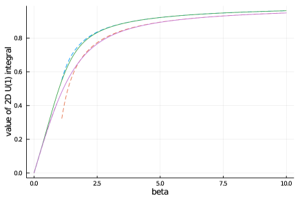
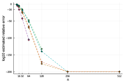
Figure 3: Illustration of numerical results for the 2D compact $U(1)$ lattice gauge theory. Left: Comparison of our FFT based algorithm (solid lines) with two known asymptotical formulae for $\beta\ll 1$ and $\beta\gg 1$ (dashed lines); the top curve is for $L=2$ and the bottom curve is for $L=200$. Right: Estimated accuracy showing exponential convergence for increasing $n$ compared to our final calculated value with $n=1024$ for all combinations of $L\in\{2,20,200\}$ and $\beta\in\{1,4,8\}$ (see text).

In the left hand side of Figure 3 we compare our calculated values to a known asymptotic formula for $\beta\ll 1$ from [5] and $\beta\gg 1$ from [22] for the 2D compact $U(1)$ lattice gauge integral for $L=2$ and $L=200$. We can see that for small values of $\beta$ and for large values of $\beta$ the asymptotic formulae are close to our calculated values, while in the neighbourhood of $\beta=1$ the asymptotic formulae deviate more, as expected.

In the right hand side of Figure 3 we illustrate the accuracy of our method in terms of $n$. To calculate a reference value for different values of $L$ and $\beta$ we have run our code with $n=1024$ and increased the precision of Julia’s BigFloat type to approximately $200$ decimal digits. We plot the base $10$ logarithm of the estimated relative error (using the reference value for $n=1024$) in terms of $n$ on the horizontal axis in linear scale. We plot the error for all combinations of $L\in\{2,20,200\}$ and $\beta\in\{1,4,8\}$. The missing data points are when the error was zero. Since $200$ decimal digits is our maximum precision the lines will flat line at $-200$. We observed that the lines for the different values of $L$ are always close together and hence we conclude that the value of $L$ does not really matter for the performance of the algorithm. For the different choices of $\beta$ we observed that larger values of $\beta$ make the problem slightly harder. E.g., the lines for $\beta=8$ are the ones on top with the slowest decay, while the lines for $\beta=1$ are the ones at the bottom with the fastest decay. This is not a surprise, and obviously, the limiting case of $\beta=0$ is the trivial problem. All cases show exponential convergence, this is why we resorted to arbitrary precision to make the graph. If one is only interested in double precision results, i.e., a relative error of about $10^{-16}$, then we see from the graph that $n=32$ is sufficient to give $16$ decimal digits for the large $\beta=8$, while $n=16$ would suffice for $\beta=1$. From the graph we also see that with $n$ somewhere between $128$ and $256$ we can expect to have more than $200$ digits decimal precision for any of the $\beta$’s and $L$’s that we plotted.

Calculating all the results for the $101$ $\beta$ values and $3$ $L$ values from the Julia code snippet above in double precision with $n=32$ takes less than $10$ milliseconds on a MacBook Pro from 2013 (2.6 Ghz Dual-Core Intel Core i5).

6.2 2D higher order couplings

The denominator in the Wilson loop (2.2) can be expressed as

$$\int_{D^{L^{2}}}\int_{D^{L^{2}}}\prod_{i=0}^{L-1}\underbrace{\prod_{j=0}^{L-1}f_{i,j}\Big{(}\textstyle\sum_{k=0}^{r_{a}}\big{(}x^{a}_{i+k,j}-x^{a}_{i+k,j+r_{b}}\big{)}+\textstyle\sum_{k=0}^{r_{b}}\big{(}x^{b}_{i+r_{a},j+k}-x^{b}_{i,j+k}\big{)}\Big{)}}_{=:\,g_{i}\big{(}(\boldsymbol{x}_{i}^{a},\boldsymbol{x}_{i+1}^{a},\ldots,\boldsymbol{x}_{i+r_{a}}^{a});\,\boldsymbol{x}^{b}\big{)}}\,\mathrm{d}\boldsymbol{x}^{a}\,\mathrm{d}\boldsymbol{x}^{b}$$

$$\,=\,\int_{D^{L^{2}}}\bigg{(}\int_{D^{L^{2}}}\prod_{i=0}^{L-1}g_{i}\Big{(}(\boldsymbol{x}_{i}^{a},\boldsymbol{x}_{i+1}^{a},\ldots,\boldsymbol{x}_{i+r_{a}}^{a});\boldsymbol{x}^{b}\Big{)}\,\mathrm{d}\boldsymbol{x}^{a}\bigg{)}\mathrm{d}\boldsymbol{x}^{b}.$$

Assuming that $L$ is a multiple of $r_{a}$, the inner integral has order $r_{a}$ coupling and can be turned into an $L/r_{a}$-fold product of $r_{a}L$-dimensional integrals following Section 4. We can use an $N$-point lattice rule in $r_{a}L$ dimensions as in Scenario (B4) at the cost of order $(L/r_{a})\,N^{3}$ times the number of different samples of $\boldsymbol{x}^{b}$. The outer integral over $\boldsymbol{x}^{b}$ cannot be simplified so it is of dimensionality $L^{2}$. This problem is truly high dimensional, except for the special case $r_{a}=r_{b}=1$ which can be simplified as we show in Corollary 2 in Appendix A using Fourier series.

6.3 3D first order couplings

The 3D compact $\mathit{U}(1)$ lattice gauge theory problem (2.2) is very tough. We show in Lemma 5 in Appendix A that there is an explicit expression in terms of Fourier coefficients. Further work is needed to see how this expression can be used to simplify the integral calculations.

7 Summary

In this paper we developed efficient recursive strategies to tackle a class of high dimensional integrals having a special product structure with low order couplings, motivated by physics models such as the quantum rotor and the 2D compact $U(1)$ lattice gauge theory (Section 2). We reviewed and extended the recursive strategy from [1, 17] for generic integrals with first order couplings (not necessarily from physics) to identify scenarios that enable the use of FFT for efficient computation as well as the use of lattice cubature rules when we have an $L$-fold product of $s$-dimensional integrals (Section 3). Furthermore, we extended the recursive strategy to higher order couplings, noting that the problems can become truly high dimensional (Section 4). Then we considered particular physics applications (Sections 5 and 6) and provided Julia codes for the special cases of quantum rotor and 2D compact $U(1)$ lattice gauge theory. Finally we provided an alternative formulation of the integrals in terms of Fourier series to pave the way for future work for tough 2D and 3D physics problems (Appendix).

Acknowledgements

We gratefully acknowledge the financial support from the Australian Research Council under grant DP180101356 and the Research Foundation Flanders (FWO) under grant G091920N.

Appendix A Alternative approach via Fourier series

A.1 1D problems

Lemma 3

Let $f_{i}:D\to{\mathbb{R}}$ be periodic and have an absolutely convergent Fourier series, and assume parametric periodicity $x_{i}=x_{i\bmod L}$. Then

$$\int_{D^{L}}\prod_{i=0}^{L-1}f_{i}\big{(}x_{i+1}-x_{i}\big{)}\,\mathrm{d}\boldsymbol{x}\,=\,\sum_{\ell\in{\mathbb{Z}}}\prod_{i=0}^{L-1}\widehat{f_{i}}(\ell).$$

• Define a periodic function

  $${\mathcal{I}}(\boldsymbol{y}) :=\,\int_{D^{L}}\prod_{i=0}^{L-1}f_{i}\big{(}\xi_{i}(\boldsymbol{x})+y_{i}\big{)}\,\mathrm{d}\boldsymbol{x},\qquad\boldsymbol{y}\in D^{L},$$

  for generic functions $\xi_{i}$, and consider its Fourier series

  $${\mathcal{I}}(\boldsymbol{y})\,=\,\sum_{\boldsymbol{h}\in{\mathbb{Z}}^{L}}\widehat{{\mathcal{I}}}(\boldsymbol{h})\,e^{2\pi\mathrm{i}\,\boldsymbol{h}\cdot\boldsymbol{y}},\qquad\widehat{{\mathcal{I}}}(\boldsymbol{h})\,:=\,\int_{D^{L}}{\mathcal{I}}(\boldsymbol{y})\,e^{-2\pi\mathrm{i}\,\boldsymbol{h}\cdot\boldsymbol{y}}\,\mathrm{d}\boldsymbol{y}.$$

  The desired integral is recovered by evaluating the Fourier series at $\boldsymbol{y}=\boldsymbol{0}$: ${\mathcal{I}}(\boldsymbol{0})\,=\,\sum_{\boldsymbol{h}\in{\mathbb{Z}}^{L}}\widehat{{\mathcal{I}}}(\boldsymbol{h})$.

  We proceed to compute the Fourier coefficients $\widehat{{\mathcal{I}}}(\boldsymbol{h})$. Due to the product structure, all integrals in $\widehat{{\mathcal{I}}}(\boldsymbol{h})$ are one-dimensional

  $$\int_{D}f_{i}\big{(}\xi_{i}(\boldsymbol{x})+y_{i}\big{)}\,e^{-2\pi\mathrm{i}\,h_{i}\,y_{i}}\,\mathrm{d}y_{i}\,=\,\int_{D}\sum_{\ell\in{\mathbb{Z}}}\widehat{f_{i}}(\ell)\,e^{2\pi\mathrm{i}\,\ell\,(\xi_{i}(\boldsymbol{x})+y_{i})}\,e^{-2\pi\mathrm{i}\,h_{i}\,y_{i}}\,\mathrm{d}y_{i}$$

  $$\,=\,\sum_{\ell\in{\mathbb{Z}}}\widehat{f_{i}}(\ell)\,e^{2\pi\mathrm{i}\,\ell\,\xi_{i}(\boldsymbol{x})}\int_{D}e^{2\pi\mathrm{i}\,(\ell-h_{i})\,y_{i}}\,\mathrm{d}y_{i}\,=\,\widehat{f_{i}}(h_{i})\,e^{2\pi\mathrm{i}\,h_{i}\,\xi_{i}(\boldsymbol{x})},$$ (32)

  where we used $\int_{D}e^{2\pi\mathrm{i}(\ell-h)y}\,\mathrm{d}y=1$ if $\ell=h$ and is $0$ otherwise. Thus

  $$\widehat{{\mathcal{I}}}(\boldsymbol{h}) \,=\,\int_{D^{L}}\prod_{i=0}^{L-1}\widehat{f_{i}}(h_{i})\,e^{2\pi\mathrm{i}\,h_{i}\,\xi_{i}(\boldsymbol{x})}\,\mathrm{d}\boldsymbol{x}\,=\,\bigg{(}\prod_{i=0}^{L-1}\widehat{f_{i}}(h_{i})\bigg{)}\int_{D^{L}}e^{2\pi\mathrm{i}\,\sum_{i=0}^{L-1}h_{i}\,\xi_{i}(\boldsymbol{x})}\,\mathrm{d}\boldsymbol{x}.$$

  Specializing now to $\xi_{i}(\boldsymbol{x}):=x_{i+1}-x_{i}$, we have for the exponent

  $$\sum_{i=0}^{L-1}h_{i}\,\xi_{i}(\boldsymbol{x})\,=\,\sum_{i=0}^{L-1}h_{i}\,x_{i+1}-\sum_{i=0}^{L-1}h_{i}\,x_{i}\,=\,\sum_{i=0}^{L-1}h_{i-1}\,x_{i}-\sum_{i=0}^{L-1}h_{i}\,x_{i}\,=\,\sum_{i=0}^{L-1}(h_{i-1}-h_{i})\,x_{i},$$

  where in the second equality we re-indexed the first sum using the property that all indices are taken modulo $L$. Thus $\int_{D^{L}}e^{2\pi\mathrm{i}\,\sum_{i=0}^{L-1}h_{i}\,\xi_{i}(\boldsymbol{x})}\,\mathrm{d}\boldsymbol{x}=1$ if and only if

  $$h_{i-1}=h_{i}\qquad\mbox{for all $i$ (taken modulo $L$)},$$ (33)

  and the integral is zero otherwise. We conclude that all components of $\boldsymbol{h}$ must be the same for the corresponding Fourier coefficient to be nonzero. Hence

  $${\mathcal{I}}(\boldsymbol{y})\,=\,\sum_{\ell\in{\mathbb{Z}}}\bigg{(}\prod_{i=0}^{L-1}\widehat{f_{i}}(\ell)\bigg{)}\,e^{2\pi\mathrm{i}\,(\ell,\ldots,\ell)\cdot\boldsymbol{y}}.$$

  Our desired integral is recovered by evaluating the Fourier series at $\boldsymbol{y}=\boldsymbol{0}$. $\hfill\Box$

The result can be extended to higher order couplings by changing the definition of the functions $\xi_{i}$ in the proof.

Corollary 1

Let $f_{i}:D\to{\mathbb{R}}$ be periodic and have an absolutely convergent Fourier series, and assume parametric periodicity $x_{i}=x_{i\bmod L}$. Then

$$\int_{D^{L}}\prod_{i=0}^{L-1}f_{i}\big{(}x_{i+1}-x_{i-1}\big{)}\,\mathrm{d}\boldsymbol{x}\,=\,\begin{cases}\displaystyle\sum_{\ell\in{\mathbb{Z}}}\prod_{i=0}^{L-1}\widehat{f_{i}}(\ell)&\mbox{if $L$ is odd},\\ \displaystyle\bigg{(}\sum_{\ell\in{\mathbb{Z}}}\prod_{\stackrel{{\scriptstyle\scriptstyle{i=0}}}{{\scriptstyle{\rm even}}}}^{L-1}\widehat{f_{i}}(\ell)\bigg{)}\bigg{(}\sum_{\ell\in{\mathbb{Z}}}\prod_{\stackrel{{\scriptstyle\scriptstyle{i=0}}}{{\scriptstyle{\rm odd}}}}^{L-1}\widehat{f_{i}}(\ell)\bigg{)}&\mbox{if $L$ is even}.\end{cases}$$

• We replace the functions $\xi_{i}$ in the proof of Lemma 3 by $\xi_{i}(\boldsymbol{x}):=x_{i+1}-x_{i-1}$. Then the condition (33) becomes

  $$h_{i-1}=h_{i+1}\qquad\mbox{for all $i$ (taken modulo $L$)}.$$

  We conclude that if $L$ is odd then all components of $\boldsymbol{h}$ must be equal, and if $L$ is even then there are two possible values for the components of $\boldsymbol{h}$ depending on whether the index is even or odd. This leads to the corollary. $\hfill\Box$

A.2 2D problems

The same strategy can be used to tackle 2D problems.

Lemma 4

Let $f_{i,j}:D\to{\mathbb{R}}$ be periodic and have an absolutely convergent Fourier series, and assume parametric periodicity modulo $L$. Then

$$\int_{D^{L^{2}}}\int_{D^{L^{2}}}\prod_{i=0}^{L-1}\prod_{j=0}^{L-1}f_{i,j}\big{(}x^{a}_{i,j}-x^{a}_{i,j+1}-x^{b}_{i,j}+x^{b}_{i+1,j}\big{)}\,\mathrm{d}\boldsymbol{x}^{a}\,\mathrm{d}\boldsymbol{x}^{b}\,=\,\sum_{\ell\in{\mathbb{Z}}}\prod_{i=0}^{L-1}\prod_{j=0}^{L-1}\widehat{f_{i,j}}(\ell).$$

• As in the 1D problem we define

  $${\mathcal{I}}(\boldsymbol{y}) \,:=\,\int_{D^{L^{2}}}\int_{D^{L^{2}}}\prod_{i=0}^{L-1}\prod_{j=0}^{L-1}f_{i,j}\big{(}\xi_{i,j}(\boldsymbol{x}^{a},\boldsymbol{x}^{b})+y_{i,j}\big{)}\,\mathrm{d}\boldsymbol{x}^{a}\,\mathrm{d}\boldsymbol{x}^{b},\qquad\boldsymbol{y}\in D^{L^{2}},$$

  for generic functions $\xi_{i,j}$, and consider the Fourier series

  $${\mathcal{I}}(\boldsymbol{y})\,=\,\sum_{\boldsymbol{h}\in{\mathbb{Z}}^{L^{2}}}\widehat{{\mathcal{I}}}(\boldsymbol{h})\,e^{2\pi\mathrm{i}\,\boldsymbol{h}\cdot\boldsymbol{y}},\qquad\widehat{{\mathcal{I}}}(\boldsymbol{h})\,:=\,\int_{D^{L^{2}}}{\mathcal{I}}(\boldsymbol{y})\,e^{-2\pi\mathrm{i}\,\boldsymbol{h}\cdot\boldsymbol{y}}\,\mathrm{d}\boldsymbol{y},$$

  where for the dot product we interpret an element in $D^{L^{2}}$ as a vector of length $L^{2}$ rather than as a matrix of $L\times L$. Our desired integral is recovered by evaluating the Fourier series at $\boldsymbol{y}=\boldsymbol{0}$.

  Analogously to (Proof.), all integrals in $\widehat{{\mathcal{I}}}(\boldsymbol{h})$ are one-dimensional

  $$\int_{D}f_{i,j}\big{(}\xi_{i,j}(\boldsymbol{x}^{a},\boldsymbol{x}^{b})+y_{i,j}\big{)}\,e^{-2\pi\mathrm{i}\,h_{i,j}\,y_{i,j}}\,\mathrm{d}y_{i,j}\,=\,\widehat{f_{i,j}}(h_{i,j})\,e^{2\pi\mathrm{i}\,h_{i,j}\,\xi_{i,j}(\boldsymbol{x}^{a},\boldsymbol{x}^{b})},$$

  and thus

  $$\widehat{{\mathcal{I}}}(\boldsymbol{h}) \,=\,\bigg{(}\prod_{i=0}^{L-1}\prod_{j=0}^{L-1}\widehat{f_{i,j}}(h_{i,j})\bigg{)}\int_{D^{L^{2}}}\int_{D^{L^{2}}}e^{2\pi\mathrm{i}\,\sum_{i=0}^{L-1}\sum_{j=0}^{L-1}h_{i,j}\,\xi_{i,j}(\boldsymbol{x}^{a},\boldsymbol{x}^{b})}\,\mathrm{d}\boldsymbol{x}^{a}\,\mathrm{d}\boldsymbol{x}^{b}.$$ (34)

  Specializing now to $\xi_{i,j}(\boldsymbol{x}^{a},\boldsymbol{x}^{b})\,:=\,x^{a}_{i,j}-x^{a}_{i,j+1}-x^{b}_{i,j}+x^{b}_{i+1,j}$, we have the exponent

  $$\sum_{i=0}^{L-1}\sum_{j=0}^{L-1}h_{i,j}\,\xi_{i,j}(\boldsymbol{x}^{a},\boldsymbol{x}^{b}) \,=\,\sum_{i=0}^{L-1}\sum_{j=0}^{L-1}\Big{[}\big{(}h_{i,j}-h_{i,j-1}\big{)}\,x^{a}_{i,j}-\big{(}h_{i,j}-h_{i-1,j}\big{)}\,x^{b}_{i,j}\Big{]},$$

  where we re-indexed some terms since all indices should be taken modulo $L$. We conclude that

  $$\int_{D^{L^{2}}}\int_{D^{L^{2}}}e^{2\pi\mathrm{i}\,\sum_{i=0}^{L-1}\sum_{j=0}^{L-1}h_{i,j}\,\xi_{i,j}(\boldsymbol{x}^{a},\boldsymbol{x}^{b})}\,\mathrm{d}\boldsymbol{x}^{a}\,\mathrm{d}\boldsymbol{x}^{b}$$

  $$\,=\,\prod_{i=0}^{L-1}\prod_{j=0}^{L-1}\bigg{[}\bigg{(}\int_{D}e^{2\pi\mathrm{i}(h_{i,j}-h_{i,j-1})\,x^{a}_{i,j}}\,\mathrm{d}x^{a}_{i,j}\bigg{)}\bigg{(}\int_{D}e^{-2\pi\mathrm{i}(h_{i,j}-h_{i-1,j})\,x^{b}_{i,j}}\,\mathrm{d}x^{b}_{i,j}\bigg{)}\bigg{]},$$

  which is equal to $1$ if and only if

  $$h_{i,j}=h_{i,j-1}=h_{i-1,j}\qquad\mbox{for all $i,j$ (taken modulo $L$)},$$

  and the integral is equal to $0$ otherwise. This means that all components of $\boldsymbol{h}$ are equal, and we have reduced $L^{2}$ parameters down to $1$. This yields the desired formula. $\hfill\Box$

The result extends trivially to the Wilson loop with $r_{a}=r_{b}=1$.

Corollary 2

Let $f_{i,j}:D\to{\mathbb{R}}$ be periodic and have an absolutely convergent Fourier series, and assume parametric periodicity modulo $L$. The Wilson loop with parameters $r_{a}$ and $r_{b}$ requires

$${\mathcal{I}}^{r_{a},r_{b}} \,:=\,\int_{D^{L^{2}}}\int_{D^{L^{2}}}\prod_{i=0}^{L-1}\prod_{j=0}^{L-1}f_{i,j}\big{(}\xi_{i,j}(\boldsymbol{x}^{a},\boldsymbol{x}^{b})\big{)}\,\mathrm{d}\boldsymbol{x}^{a}\,\mathrm{d}\boldsymbol{x}^{b},$$

$$\xi_{i,j}(\boldsymbol{x}^{a},\boldsymbol{x}^{b}) \,:=\,x^{a}_{i,j}+x^{a}_{i+1,j}+\cdots+x^{a}_{i+r_{a},j}+x^{b}_{i+r_{a},j}+x^{b}_{i+r_{a},j+1}+\cdots+x^{b}_{i+r_{a},j+r_{b}}$$

$$\qquad-x^{a}_{i+r_{a},j+r_{b}}-x^{a}_{i+r_{a}-1,j+r_{b}}-\cdots-x^{a}_{i,j+r_{b}}-x^{b}_{i,j+r_{b}}-x^{b}_{i,j+r_{b}-1}-\cdots-x^{b}_{i,j}.$$

We have

$${\mathcal{I}}^{1,1}\,=\,\begin{cases}\displaystyle\sum_{\ell\in{\mathbb{Z}}}\prod_{i=0}^{L-1}\prod_{j=0}^{L-1}\widehat{f_{i,j}}(\ell)&\mbox{if $L$ is odd},\\ \displaystyle\bigg{(}\sum_{\ell\in{\mathbb{Z}}}\underbrace{\textstyle\prod_{i=0}^{L-1}\prod_{j=0}^{L-1}}_{i+j~{}\mathrm{odd}}\widehat{f_{i,j}}(\ell)\bigg{)}\bigg{(}\sum_{\ell\in{\mathbb{Z}}}\underbrace{\textstyle\prod_{i=0}^{L-1}\prod_{j=0}^{L-1}}_{i+j~{}\mathrm{even}}\widehat{f_{i,j}}(\ell)\bigg{)}&\mbox{if $L$ is even}.\end{cases}$$

• Following the proof of Lemma 4, the exponent $\sum_{i=0}^{L-1}\sum_{j=0}^{L-1}h_{i,j}\,\xi_{i,j}(\boldsymbol{x}^{a},\boldsymbol{x}^{b})$ is now

  $$\sum_{i=0}^{L-1}\sum_{j=0}^{L-1}\bigg{[}\sum_{k=0}^{r_{a}}\big{(}h_{i,j}\,x_{i+k,j}^{a}-h_{i,j}\,x_{i+k,j+r_{b}}^{a}\big{)}+\sum_{k=0}^{r_{b}}\big{(}h_{i,j}\,x_{i+r_{a},j+k}^{b}-h_{i,j}\,x_{i,j+k}^{b}\big{)}\bigg{]}$$

  $$\,=\,\sum_{i=0}^{L-1}\sum_{j=0}^{L-1}\bigg{[}\sum_{k=0}^{r_{a}}\big{(}h_{i-k,j}-h_{i-k,j-r_{b}}\big{)}\,x_{i,j}^{a}+\sum_{k=0}^{r_{b}}\big{(}h_{i-r_{a},j-k}-h_{i,j-k}\big{)}\,x_{i,j+k}^{b}\bigg{]},$$

  where we again re-indexed some terms. We conclude that the integral in (34) is equal to $1$ if and only if for all $i,j$ (taken modulo $L$)

  $$\sum_{k=0}^{r_{a}}h_{i-k,j}\,=\,\sum_{k=0}^{r_{a}}h_{i-k,j-r_{b}}\qquad\mbox{and}\qquad\sum_{k=0}^{r_{b}}h_{i,j-k}\,=\,\sum_{k=0}^{r_{b}}h_{i-r_{a},j-k},$$ (35)

  and is $0$ otherwise. For the special case $r_{a}=r_{b}=1$, the conditions in (35) are

  $$\begin{cases}h_{i,j}+h_{i-1,j}\,=\,h_{i,j-1}+h_{i-1,j-1},\\ h_{i,j}+h_{i,j-1}\,=\,h_{i-1,j}+h_{i-1,j-1}.\end{cases}$$

  Adding and subtracting these two expressions lead to, respectively,

  $$h_{i,j}=h_{i-1,j-1}\qquad\mbox{and}\qquad h_{i-1,j}=h_{i,j-1}.$$

  If $L$ is a multiple of $2$, then we conclude that the components of $\boldsymbol{h}$ can take only two possible values depending on the value of $(i+j)\bmod 2$, following a chessboard pattern. On the other hand, if $L$ is not a multiple of $2$ then all components of $\boldsymbol{h}$ have the same value. These lead to the formulas in the corollary. $\hfill\Box$

A.3 3D problems

Lemma 5

Let $f_{i,j,k}:D\to{\mathbb{R}}$ be periodic and have an absolutely convergent Fourier series, and assume parametric periodicity modulo $L$. Then

$$\int_{D^{3L^{3}}}\prod_{i=0}^{L-1}\prod_{j=0}^{L-1}\prod_{k=0}^{L-1}\Big{[}f_{i,j,k}\big{(}x^{a}_{i,j,k}-x^{a}_{i,j+1,k}-x^{b}_{i,j,k}+x^{b}_{i+1,j,k}\big{)}$$

$$\qquad\qquad\qquad\qquad\cdot f_{i,j,k}\big{(}x^{c}_{i,j,k}-x^{c}_{i+1,j,k}-x^{a}_{i,j,k}+x^{a}_{i,j,k+1}\big{)}$$

$$\qquad\qquad\qquad\qquad\cdot f_{i,j,k}\big{(}x^{b}_{i,j,k}-x^{b}_{i,j,k+1}-x^{c}_{i,j,k}+x^{c}_{i,j+1,k}\big{)}\Big{]}\,\mathrm{d}\boldsymbol{x}$$

$$\,=\,\sum_{\boldsymbol{h}\in\mathcal{H}}\prod_{i=0}^{L-1}\prod_{j=0}^{L-1}\prod_{k=0}^{L-1}\Big{(}\widehat{f_{i,j,k}}(h^{a}_{i,j,k})\,\widehat{f_{i,j,k}}(h^{b}_{i,j,k})\,\widehat{f_{i,j,k}}(h^{c}_{i,j,k})\Big{)},$$

where $\boldsymbol{h}=(\boldsymbol{h}^{a},\boldsymbol{h}^{b},\boldsymbol{h}^{c})\in\mathcal{H}\subset{\mathbb{Z}}^{3L^{3}}$ satisfies for all $i,j,k$ modulo $L$,

$$\begin{cases}h^{c}_{i,j,k}-h^{c}_{i,j-1,k}-h^{b}_{i,j,k}+h^{b}_{i,j,k-1}\,=\,0,\\ h^{a}_{i,j,k}-h^{a}_{i,j,k-1}-h^{c}_{i,j,k}+h^{c}_{i-1,j,k}\,=\,0,\\ h^{b}_{i,j,k}-h^{b}_{i-1,j,k}-h^{a}_{i,j,k}+h^{a}_{i,j-1,k}\,=\,0.\end{cases}$$ (36)

• Generalizing the 1D and 2D arguments, we define for $\boldsymbol{y}=(\boldsymbol{y}^{a},\boldsymbol{y}^{b},\boldsymbol{y}^{c})\in D^{3L^{3}}$,

  $${\mathcal{I}}(\boldsymbol{y}) \,:=\,\int_{D^{3L^{3}}}\prod_{i=0}^{L-1}\prod_{j=0}^{L-1}\prod_{k=0}^{L-1}\Big{[}f_{i,j,k}\big{(}x^{a}_{i,j,k}-x^{a}_{i,j+1,k}-x^{b}_{i,j,k}+x^{b}_{i+1,j,k}+y^{c}_{i,j,k}\big{)}$$

  $$\qquad\qquad\qquad\qquad\qquad\cdot f_{i,j,k}\big{(}x^{c}_{i,j,k}-x^{c}_{i+1,j,k}-x^{a}_{i,j,k}+x^{a}_{i,j,k+1}+y^{b}_{i,j,k}\big{)}$$

  $$\qquad\qquad\qquad\qquad\qquad\cdot f_{i,j,k}\big{(}x^{b}_{i,j,k}-x^{b}_{i,j,k+1}-x^{c}_{i,j,k}+x^{c}_{i,j+1,k}+y^{a}_{i,j,k}\big{)}\Big{]}\,\mathrm{d}\boldsymbol{x}.$$

  For each $\boldsymbol{h}=(\boldsymbol{h}^{a},\boldsymbol{h}^{b},\boldsymbol{h}^{c})\in{\mathbb{Z}}^{3L^{3}}$, we compute the Fourier coefficient of ${\mathcal{I}}(\boldsymbol{y})$ to arrive at

  $$\widehat{{\mathcal{I}}}(\boldsymbol{h}) =\bigg{[}\prod_{i=0}^{L-1}\prod_{j=0}^{L-1}\prod_{k=0}^{L-1}\Big{(}\widehat{f_{i,j,k}}(h^{a}_{i,j,k})\,\widehat{f_{i,j,k}}(h^{b}_{i,j,k})\,\widehat{f_{i,j,k}}(h^{c}_{i,j,k})\Big{)}\bigg{]}\int_{D^{3L^{3}}}e^{2\pi\mathrm{i}\,p(\boldsymbol{h},\boldsymbol{x})}\,\mathrm{d}\boldsymbol{x},$$

  $$p(\boldsymbol{h},\boldsymbol{x}) =\sum_{i=0}^{L-1}\sum_{j=0}^{L-1}\sum_{k=0}^{L-1}\Big{[}\Big{(}h^{c}_{i,j,k}-h^{c}_{i,j-1,k}-h^{b}_{i,j,k}+h^{b}_{i,j,k-1}\Big{)}\,x^{a}_{i,j,k}$$

  $$\quad+\big{(}h^{a}_{i,j,k}-h^{a}_{i,j,k-1}-h^{c}_{i,j,k}+h^{c}_{i-1,j,k}\big{)}\,x^{b}_{i,j,k}+\big{(}h^{b}_{i,j,k}-h^{b}_{i-1,j,k}-h^{a}_{i,j,k}+h^{a}_{i,j-1,k}\big{)}\,x^{c}_{i,j,k}\Big{]}.$$

  We conclude that $\int_{D^{3L^{3}}}e^{2\pi\mathrm{i}\,p(\boldsymbol{h},\boldsymbol{x})}\,\mathrm{d}\boldsymbol{x}$ is equal to $1$ if and only if $\boldsymbol{h}$ belongs to a restricted index set $\mathcal{H}\subset{\mathbb{Z}}^{3L^{3}}$, satisfying (36) for all indices $i,j,k$ modulo $L$, and the integral is equal to $0$ otherwise. We obtain the required formula by taking ${\mathcal{I}}(\boldsymbol{0})=\sum_{\boldsymbol{h}\in{\mathbb{Z}}^{3L^{3}}}\widehat{{\mathcal{I}}}(\boldsymbol{h})$. $\hfill\Box$

References

• [1] A. Ammon, A. Genz, T. Hartung, K. Jansen, H. Leövey, J. Volmer, On the efficient numerical solution of lattice systems with low-order couplings, Comput. Phys. Commun. 198 (2016), 71–81.
• [2] A. Ammon, T. Hartung, K. Jansen, H. Leövey, A. Griewank, M. Müller-Preussker, Applicability of Quasi-Monte Carlo for lattice systems, PoS LATTICE 2013 (2014), 040.
• [3] A. Ammon, T. Hartung, K. Jansen, H. Leövey, J. Volmer, Overcoming the sign problem in one-dimensional QCD by new integration rules with polynomial exactness, Phys. Rev. D 94 (2016), 114508.
• [4] A. Ammon, T. Hartung, K. Jansen, H. Leövey, J. Volmer, New polynomially exact integration rules on $\mathit{U}(N)$ and $\mathit{SU}(N)$, PoS LATTICE 2016 (2016), 334.
• [5] R. Balian, J. M. Drouffe and C. Itzykson, Gauge Fields on a Lattice. 3. Strong Coupling Expansions and Transition Points, Phys. Rev. D 11 (1975) 2104. Erratum: [Phys. Rev. D 19 (1979) 2514].
• [6] S. Borowka, G. Heinrich, S. Jahn, S. P. Jones, M. Kerner and J. Schlenk, A GPU compatible quasi-Monte Carlo integrator interfaced to pySecDec, Comput. Phys. Commun. 240 (2019) 120–137.
• [7] W. Bietenholz, R. Brower, S. Chandrasekharan and U. J. Wiese, Perfect lattice topology: The Quantum rotor as a test case, Phys. Lett. B 407 (1997), 283.
• [8] W. Bietenholz, U. Gerber, M. Pepe and U.-J. Wiese, Topological Lattice Actions, JHEP 1012 (2010), 020.
• [9] H. Bungartz and M. Griebel, Sparse grids, Acta Numer. 13 (2004), 147–269.
• [10] R. E. Caflisch, W. Morokoff, and A.B. Owen, Valuation of mortgage backed securities using Brownian bridges to reduce effective dimension, J. Comput. Finance 1 (1997), 27–46.
• [11] P. Craig, A new reconstruction of multivariate normal orthant probabilities, J. R. Statist. Soc. B 70 (2008), 227–243.
• [12] E. de Doncker, A. Almulihi and F. Yuasa, High-speed evaluation of loop integrals using lattice rules, J. Phys. Conf. Ser. 1085 (2018), no. 5, 052005.
• [13] J. Dick, F. Y. Kuo, I. H. Sloan, High-dimensional integration: the Quasi-Monte Carlo way, Acta Numer., 22 (2013), 133–288.
• [14] J. Dick, F. Pillichshammer, Digital Nets and Sequences, Cambridge University Press, Cambridge, 2010.
• [15] C. Gattringer and C. B. Lang, Quantum chromodynamics on the lattice, Lect. Notes Phys.  788 (2010), 1.
• [16] A. Genz, D. K. Kahaner, The numerical evaluation of certain multivariate normal integrals, J. Comput. Appl. Math. 16 (1986), 255–258.
• [17] T. Hartung, K. Jansen, H. Leövey and J. Volmer, Avoiding the sign-problem in lattice field theory, in Monte Carlo and Quasi-Monte Carlo Methods 2018 (B. Tuffin and P. L’Ecuyer, eds), Springer Proceedings in Mathematics & Statistics, vol 324, 2020, pp. 231–249.
• [18] T. Hartung and K. Jansen, Zeta-regularized vacuum expectation values, J. Math. Phys.  60 (2019), no. 9, 093504.
• [19] A. J. Hayter, Recursive integration methodologies with statistical applications, J. Statist. Plann. Inference 136 (2006), 2284–2296.
• [20] A. J. Hayter, Recursive integration methodologies with applications to the evaluation of multivariate normal probabilities, J. Stat. Theory Pract. 5 (2011), 563–589.
• [21] F. J. Hickernell, Lattice rules: How well do they measure up?, in: Random and Quasi-Random Point Sets (P. Hellekalek and G. Larcher, eds.), Springer, Berlin, 1998, pp. 109–166.
• [22] R. Horsley and U. Wolff, Weak Coupling Expansion of Wilson Loops in Compact QED, Phys. Lett.  105B (1981), 290.
• [23] K. Jansen, Lattice QCD: A Critical status report, PoS LATTICE 2008 (2008), 010.
• [24] K. Jansen and T. Hartung, Zeta-regularized vacuum expectation values from quantum computing simulations, PoS LATTICE 2019 (2020), 363.
• [25] K. Jansen, H. Leovey, A. Ammon, A. Griewank, M. Müller-Preussker, Quasi-Monte Carlo methods for lattice systems: a first look, Comput. Phys. Commun. 185 (2014), 948–959.
• [26] C. Lemieux, Monte Carlo and Quasi-Monte Carlo Sampling, Springer, New York, 2009.
• [27] H. Niederreiter, Random Number Generation and Quasi-Monte Carlo Methods, SIAM, 1992.
• [28] D. Nuyens, The construction of good lattice rules and polynomial lattice rules, in: Uniform Distribution and Quasi-Monte Carlo Methods (P. Kritzer, H. Niederreiter, F. Pillichshammer, A. Winterhof, eds.), Radon Series on Computational and Applied Mathematics Vol. 15, De Gruyter, 2014, pp. 223–256.
• [29] I. H. Sloan, S. Joe, Lattice Methods for Multiple Integration, Oxford University Press, Oxford, 1994.
• [30] M. Troyer, U.-J. Wiese, Computational complexity and fundamental limitations to fermionic quantum Monte Carlo simulations, Phys. Rev. Lett. 94 (2005), 170201.