Vacuum fermionic currents in braneworld models
on AdS bulk with a cosmic string
Abstract
We investigate the effects of a brane and magnetic-flux-carrying cosmic string on the vacuum expectation value (VEV) of the current density for a charged fermionic field in the background geometry of (4+1)-dimensional anti–de Sitter (AdS) spacetime. The brane is parallel to the AdS boundary and the cosmic string is orthogonal to the brane. Two types of boundary conditions are considered on the brane that include the MIT bag boundary condition and the boundary conditions in -symmetric braneworld models. The brane divides the space into two regions with different properties of the vacuum state. The only nonzero component of the current density is along the azimuthal direction and in both the regions the corresponding VEV is decomposed into the brane-free and brane-induced contributions. The latter vanishes on the string and near the string the total current is dominated by the brane-free part. At large distances from the string and in the region between the brane and AdS horizon the decay of the brane-induced current density, as a function of the proper distance, is power-law for both massless and massive fields. For a massive field this behavior is essentially different from that in the Minkowski bulk. In the region between the brane and AdS boundary the large-distance decay of the current density is exponential. Depending on the boundary condition on the brane, the brane-induced contribution is dominant or subdominant in the total current density at large distances from the string. By using the results for fields realizing two inequivalent irreducible representations of the Clifford algebra, the vacuum current density is investigated in - and -symmetric fermionic models. Applications are given for a cosmic string in the Randall-Sundrum-type braneworld model with a single brane.
Keywords: Cosmic string, AdS space, Brane, Vacuum polarization
1 Introduction
The anti-de Sitter (AdS) spacetime is one of the most interesting solutions of General Relativity. The relevance of this maximally symmetric geometry from the point of view of quantum field theory resides in the fact that a large number of field theoretical problems are exactly soluble on its background. This allows to reveal information on the influence of gravitational field on quantum matter in less symmetric geometries. In addition, the length scale related to the AdS constant curvature, can serve as a regularization parameter for infrared divergences in interacting quantum field theories without reducing the number of symmetries [1]. The AdS spacetime has been the subject of considerable attention due to the realization that it emerges as a stable ground state solution in Kaluza-Klein models, extended supergravity and string theories and approximates the near-horizon geometries of extremal black holes, domain walls and -brane configurations in string theories. In addition, the AdS background geometry plays a crucial role in the AdS/CFT correspondence and braneworlds models with large extra dimensions. These two exciting developments of modern theoretical physics naturally appear in the string/M-theory context and offer an interesting framework to approach several problems in particle physics, cosmology and condensed matter physics. Motivated by the points given above, quantum field theory in AdS background has been extensively studied by several authors (see, for instance, [2]-[23] and references therein).
In the present paper we investigate the effects of a cosmic string and brane on the vacuum expectation value (VEV) of the fermionic current density induced by a magnetic flux tube in AdS spacetime. Cosmic strings are among the most interesting types of topological defects that might have formed as a consequence of spontaneous symmetry breaking at phase transitions in the early Universe [24, 25, 26]. As possible seeds for large scale structure formation in the Universe, they have been extensively studied in the eighties and early nineties of the last century. Although the observational data on the temperature anisotropies of the cosmic microwave background radiation (CMB) supported the inflationary scenario for the density perturbations, excluding the cosmic strings as the main origin of structures, they are still sources for a number of interesting physical effects. The latter include the gravitational lensing, creation of small non-Gaussianities in the CMB, the generation of gravitational waves, gamma ray bursts and high-energy cosmic rays.
Initially, cosmic strings have been regarded as completely different from fundamental superstrings. In string theory the latter are considered as the basic building blocks of matter. A particularly interesting topic in recent developments of the subject is the investigation of possibility for appearance of low tension cosmic strings in string theory (see [27] for early discussion). Models were proposed where, under certain conditions, the fundamental strings can grow to macroscopic size with features similar to those for cosmic strings. Among the examples of this kind of models is the brane-inflation scenario [28] (for reviews see [29, 30, 31, 32]). In this scenario the inflation appears naturally in the braneworld context and it is a specific realization of the inflationary paradigm in the early Universe within the braneworld picture in the string theory. Among other interesting predictions in this theoretical framework, the production of cosmic strings towards the end of inflation has attracted considerable attention [33]. It has been suggested that the detection of cosmic strings could be a possible way to verify the inflationary paradigm, providing an interesting testing ground into string theory by probing the braneworld scenario before the inflationary phase [29, 30, 31, 32]. Many other publications have investigated the effects of braneworld gravity on the physics of cosmic strings [34, 35, 36, 37, 38, 39]. Specifically in [39], the authors have studied the consequences of the braneworld modified gravity on the cosmic string phenomenology. By considering the presence of a cosmic string they were able to put a strong constraint on the braneworld tension, making it compatible with the observational data for temperature anisotropies of CMB. They also have shown that the deficit angle induced in the string’s outside region is significantly attenuated due to the braneworld gravitational corrections, providing a possible explanation for the null experimental results based on the cosmic string effects caused by its conical geometry, such as lensing effects. This close relation between braneworlds and cosmic strings gives us enough motivation to consider both objects within a unified picture for studying vacuum quantum effects in the present work.
The geometry associated with a cosmic string in AdS spacetime has been analyzed in [40, 41]. There the authors have shown that, similar to the case of Minkowskian spacetime, at distances from the string larger than its core radius, the gravitational effects of the string can be approximated by a planar angle deficit in the two-dimensional subspace orthogonal to the string in the AdS line-element. The combination of non-trivial topology and the spacetime curvature induce vacuum polarization effects for quantum fields. In this sense the investigation of the influence of the presence of a cosmic string in AdS bulk on the vacuum polarization of quantum fields, have been investigated for scalar and fermionic fields in [42] and [43], respectively. Taking into account the presence of a magnetic flux along the string core, in [44] the vacuum current for a charged scalar field in AdS bulk was investigated. The VEV of the corresponding energy-momentum tensor was analyzed in [45]. Finally, in [46] the induced fermionic current in the AdS bulk in the presence of a cosmic string was discussed.111In fact, in references [44], [45] and [46], higher dimensional AdS spacetimes were considered, admitting that an extra dimension coordinate was compactified.
Here we consider the VEV of the fermionic current density around magnetic-flux-carrying cosmic string on AdS bulk in the presence of a brane parallel to the AdS boundary. The cosmic string is orthogonal to the brane and on the brane the fermionic field is constrained by two types of boundary conditions. The first one corresponds to the MIT bag boundary condition and the second one is obtained from the bag boundary condition changing the sign of the term with the normal to the boundary. In braneworld models these boundary conditions are dictated by the -symmetry under the reflection with respect to the brane. Note that the vacuum current densities on locally AdS bulk with a part of spatial dimensions compactified to a torus and in the presence of branes have been investigated in [47, 48, 49] and [50, 51, 52] for charged scalar and fermionic fields, respectively.
The paper is organized as follows. In section 2 we describe the setup of the problem and present the complete set of positive and negative energy solutions to the Dirac equation in the presence of a brane parallel to the AdS boundary. In section 3, the VEV of the current density in the region between the brane and the AdS horizon (R-region) is investigated. Various asymptotic limits are considered and numerical results are presented. Similar investigations for the region between the brane and AdS boundary (L-region) are presented in section 4. In section 5 we consider the second type of boundary condition and analyse the effects of the brane on the current densities in the R- and L-regions. Discussion of our results in the context of - and -symmetric models is presented in section 6. In section 7, an application to the Randall-Sundrum model with a single brane is provided. Section 8 summarizes the most relevant results obtained. Throughout the paper, we use natural units .
2 Problem setup and the fermionic modes
We consider a fermionic quantum field in background of -dimensional spacetime with the metric tensor defined by the line element
| (2.1) |
where , , , . For , Eq. (2.1) presents the AdS spacetime described in Poincaré coordinates (with polar coordinates in two-dimensional subspace). The parameter defines the cooresponding curvature radius and is related to negative cosmological constant and the Ricci scalar by formulas and . The limiting values of the -coordinate, and , determine the AdS boundary and the AdS horizon, respectively. In what follows we will be concerned with the case that corresponds to two-dimensional conical subspace with planar angle deficit . Note that the latter does not change the local geometry for . However, the topology is changed and this gives rise interesting effects in quantum field theory. The line element (2.1) without the term describes an idealized cosmic string in background of AdS spacetime.
In the presence of a classical gauge field , the Dirac equation for the field reads
| (2.2) |
where is the spin connection. In -dimensional spacetime the irreducible representation of the Clifford algebra is realized by Dirac matrices . In odd spacetime dimensions there are two inequivalent irreducible representations and the parameter corresponds to those representations (see the discussion in section 6 below). We assume the presence of a codimension one brane parallel to the AdS boundary and located at . On the brane the field operator is constrained by the MIT bag boundary condition
| (2.3) |
where is the corresponding normal vector. In terms of the coordinate the line element (2.1) is written in conformally flat form for . It is conformally related to the line element associated with a cosmic string in -dimensional Minkowski spacetime. The physical distance from the brane is measured in terms of the coordinate , defined as , . For the -coordinate of the brane one has . The distance from the brane is expressed as . The brane separates the background space into two regions: and . We shall refer them as L(left)- and R(right)- regions, respectively. In the coordinate system , for the normal in the boundary condition (2.3) one has in the L-region and in the R-region.
In the discussion below, the gamma matrices will be taken in the following representation:
| (2.4) |
where correspond to the coordinates . In the respective expressions matrices are defined as
| (2.5) |
with , and . These are the Pauli matrices in the coordinate system . With this choice of the gamma matrices, the product in the field equation (2.2) takes the form
| (2.6) |
In the absence of the cosmic string one has .
Our interest in the present paper is the VEV of the fermionic current density , with being the Dirac adjoint defined in terms of the flat spacetime gamma matrix . This VEV can be presented as a mode sum over complete set of positive and negative energy fermionic wave-functions , where the set of quantum numbers specifies the modes. Expanding the field operators in the expression for over the functions and by using the definition of the vacuum state one can see that
| (2.7) |
For the gauge field in (2.2) we will assume a simple configuration with constant . This corresponds to a magnetic flux along the string’s core. Hence, for evaluation of the vacuum current density one needs complete set of solutions to (2.2) for the special case of the vector potential and obeying the boundary condition (2.3).
The general procedure for solving the Dirac equation is similar to that already discussed in [43] for (3+1)-dimensional AdS spacetime and in [46] for the problem on (4+1)-dimensional AdS bulk with compactified spatial dimension. Here we will describe the main steps only. From the problem symmetry the dependence of the mode functions on the spacetime coordinates and can be taken in the standard plane wave form , where is the energy and the upper and lower signs correspond to the positive and negative energy modes. Decomposing the four-component spinor into two-component spinors and , , from the Dirac equation (2.2) we obtain two coupled first order differential equations for the upper and lower components. From that system of equations the second order differential equations are derived for the separate functions. Separating the variables and in both these equations, the corresponding functions are expressed in terms of the cylinder functions. Then, additional conditions, previously discussed in [53], are imposed that relate different components of the spinor. As a result all those manipulations, the positive and negative energy fermionic mode functions are presented as
| (2.8) |
with , , and
| (2.9) |
The orders of the functions are given by the expressions
| (2.10) |
where , for and for . In (2.8),
| (2.11) |
where and are the Bessel and Neumann functions and we have introduced the notations
| (2.12) |
Note that one of the constants and in (2.11) can be absorbed in the coefficient . With the definitions given above, the set of quantum numbers in (2.7) is specified as . It can be checked that the functions (2.8) are the eigenfunctions of the -projection of the total angular momentum with the eigenvalues :
| (2.13) |
where . The parameter in the definition of is expressed in terms of the magnetic flux along the string axis by the relation , where is the quantum of the flux.
The coefficient in (2.8) is determined from the normalization condition
| (2.14) |
where is understood as the Dirac delta function for continuous components of and the Kronecker delta for discrete ones. The integration over in (2.14) goes over in the L-region and over in the R-region. The remaining coefficient in the linear combination is determined from the boundary condition (2.3).
Note that along the azimuthal direction the mode functions (2.8) obey the periodicity condition . We could consider a more general quasiperiodicity condition with a constant phase . By the gauge transformation , , the set of the fields is transformed to the set , where the new field is periodic along the azimuthal direction. From here we conclude that the VEV of the current density for the field obeying the quasiperiodicity condition with the phase is obtained from the corresponding results given below for periodic fields by the replacement .
The properties of the vacuum state are different in the L- and R-regions and separate consideration for the fermionic current is required. We start our investigation with the R-region.
3 Current density in the R-region
In this section we consider the current density in the region (R-region).
3.1 General formula
The corresponding modes are given by (2.8), where the function is defined as (2.11). From the boundary condition (2.3) it follows that the coefficients in the corresponding linear combination can be taken as and . Hence, in the R-region the mode functions have the form (2.8), where
| (3.1) |
Here and in what follows we use the notation
| (3.2) |
The eigenvalues of the quantum number are continuous and in the normalization condition (2.14) the corresponding part in the right-hand side is understood as the delta function . In the evaluation of the normalization integral we note that for the dominant contribution to the integral over comes from large values of and we can replace the cylinder functions with the arguments by the corresponding asymptotic expressions. In this way one can see that with
| (3.3) |
and with definitions from (2.12).
Given the mode functions, the VEV of the current density in the R-region is evaluated by using the formula (2.7), where
| (3.4) |
First of all, we can see that for the mode functions (2.8) and consequently . For the components it can be seen that the product is an odd function of . By taking into account that in the formula for the VEV of the current density one has integration , we conclude that . Hence, the only nonzero component corresponds to the current density along the azimuthal direction, . The terms in the mode sum with and give the same contribution and, after summation over , the corresponding physical component is expressed as
| (3.5) | |||||
where the energy is given by (2.9). If we write the parameter in the form
| (3.6) |
where is an integer number, then, by shifting , we can see that the VEV depends on only.
For the transformation of the expression (3.5) we use the integral representation
| (3.7) |
For the evaluation of the integral over we use the formula
| (3.8) |
with . After evaluation of the -integral and introducing instead of a new integration variable , the current density is expressed as
| (3.9) | |||||
where we have introduced the notation
| (3.10) |
An alternative expression is obtained from (3.9) by using the integral representation for the function [54, 55, 56]. The latter is obtained from the representation for the series from [57]:
| (3.11) | |||||
where and
| (3.12) |
The prime on the summation sign in (3.11) means that for even values of the term with should be taken with an additional coefficient 1/2. With (3.11), after evaluating the -integral, from (3.9) we find
| (3.13) | |||||
where is the Macdonald function.
We are interested in the effect induced by the brane. In order to separate the corresponding contribution one should subtract from (3.13) the current density in the absence of the brane. The latter is evaluated by the formula (2.7) with the mode functions replaced by the functions in the brane-free geometry. Those functions are obtained from (2.8) with the function and the normalization constant
| (3.14) |
For the VEV of the azimuthal current density in the brane-free geometry this gives
| (3.15) | |||||
By transformations similar to those we have described before, this VEV is presented as
| (3.16) | |||||
Note that (3.16) is the same for and and the current densities in the brane-free geometry coincide for two inequivalent representations of the Clifford algebra.
We present the current density in the geometry with the brane in the decomposed form
| (3.17) |
where the part is induced by the brane. The corresponding integral representation is obtained by subtracting (3.16) from (3.13). We can further transform the expression for the brane-induced contribution by making use of relation
| (3.18) |
where , , are the Hankel functions. This leads to the expression
| (3.19) | |||||
As the next step we rotate the contour of the integration over by the angle () for the term with (). Introducing the modified Bessel functions one finds
| (3.20) | |||||
From (3.20) it follows that the current density is an odd function of . For a massless field one has , and the brane-induced contribution in the R-region vanishes. The charge flux through the hypersurface is expressed as , where is the normal to the hypersurface. Note that the quantity depends on through the ratios and . The first one is the proper distance from the string
| (3.21) |
measured in units of the AdS curvature radius, and the second one determines the proper distance from the brane
| (3.22) |
For half-integer values of the ratio of the magnetic flux to the flux quantum one finds
| (3.23) |
This shows that the brane-induced contribution is discontinuous at half integer values of the magnetic flux in units of the flux quantum. The same is the case for the brane-free contribution. It is of interest to note that the limiting values are linear functions of the parameter .
For the planar angle deficit is absent and from (3.19) we get
| (3.24) | |||||
This expression describes the brane-induced contribution in the current density generated by an idealized zero-thickness magnetic flux tube. We expect that it will approximate the corresponding current density for a finite thickness flux tube at distances from the tube larger than the core radius.
Note that the integral in the expression (3.16) for the current density is evaluated by using the formula [58] (in [58] there is a missprint, instead of should be )
| (3.25) |
where and is the associated Legendre function of the second kind. This gives (see also [46])
| (3.26) | |||||
with the notation
| (3.27) |
Near the string the leading term in the expansion over the distance from the string is given by
| (3.28) |
where we have introduced the notation
| (3.29) |
At large distances from the string, , the leading term in the corresponding expansion is expressed as
| (3.30) |
For a massless field the expression of the current density is simplified to
| (3.31) |
Note that for a massive field the leading term in the expansion over the distance from the string, given by (3.28), coincides with (3.31).
The VEV of the current density for cosmic string in the Minkowski bulk, , is obtained from in the limit with fixed value of the coordinate . In this limit one has and for the Bessel functions in (3.16) we can use the Debye’s asymptotic expansions [59]. This leads to the expression
| (3.32) | |||||
The integrals are evaluated by using the formula from [58] and we find
| (3.33) | |||||
For a massless field one gets . This result is conformally related to the expression (3.31) of the current density for cosmic string in the AdS bulk. For a massive field, at large distances from the string, , the current density is suppresses by the factor for and by the factor for . Recall that for the AdS bulk and at large distances from the string, the brane-free contribution in the current density decays according to inverse power-law (see (3.30)).
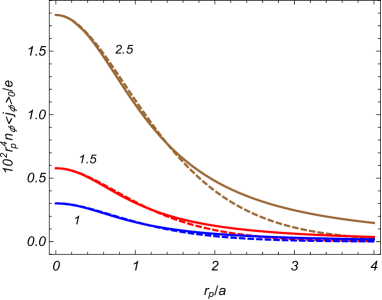
The full curves in figure 1 present the quantity for cosmic string in the AdS bulk as a function of the proper distance from the string (3.21), measured in units of the AdS curvature radius. The graphs are plotted for , , and the numbers near the curves correspond to the values of the parameter . The same quantity for cosmic string in the Minkowski is plotted in figure 1 by dashed curves. The corresponding line element is given by the expression in the brackets on the right-hand side of (2.1) and , . For both background geometries and this limiting value is equal to , , for , respectively. As noted above, near the string the leading terms in the corresponding asymptotic expansions for the AdS and Minkowski bulks coincide and in that region the effects of the background curvature are weak. As seen from the graphs and in accordance with the asymptotic analysis, those effects are essential at large distances from the cosmic string. Note that for a massless field one has (see (3.31)) for all values of in both AdS and Minkowski geometries. For the corresponding graphs will be presented by horizontal lines which touch the curves in figure 1 at .
3.2 Asymptotics of the current density and numerical results
We turn to the investigation of the current density for the geometry with a brane in asymptotic regions of the variables. Near the string, assuming that , we get
| (3.34) |
and the boundary-induced VEV behaves as . Note that on the string the brane free part diverges and, hence, it dominates for points near the string. For the investigation of the current density at large distances from the string it is convenient to use the representation (3.13). Introducing a new integration variable and assuming that , we see that the dominant contribution comes from the part of the integrand with the function . By taking into account that
| (3.35) |
to the leading order one finds
| (3.36) |
As seen, the decay of the current density at large distances from the string is power-law for both massless and massive fields. This is in contrast to the case of the Minkowski bulk, where the decay for massive fields is exponential. For a massless field the brane-induced contribution vanishes and (3.36) is reduced to (3.31). For the leading term (3.36) coincides with (3.30) and, hence, the current density at large distances is dominated by the brane-free contribution. For the field with , at large distances from the string the current density behaves as and the brane-induced contribution dominates.
Now let us consider the behavior of the current density at large distances from the brane, . Introducing in (3.20) a new integration variable , we use the asymptotic expressions for the modified Bessel functions with the argument for small values of the latter ratio [59]. It can be seen that, to the leading order, the brane induced current density is suppressed by the factor .This factor also describes the behavior of the current density for fixed when the location of the brane tends to the AdS boundary, . If in addition one has , we use the asymptotic of the Bessel function for small argument. After integrating over and for this gives
| (3.37) |
Considered as a function of the physical distance from the brane, , the brane-induced contribution is suppressed by the factor . For the leading term in the asymptotic expansion is given by
| (3.38) |
In this case, the brane-induced part tends to finite value on the AdS horizon.
For the investigation of the current density near the brane it is convenient to use the representation (3.13). In particular, the current density on the brane is directly obtained putting in the integrand . By taking into account that , we get
| (3.39) | |||||
Unlike the fermion condensate and the VEV of the energy-momentum tensor, the VEV of the current density is finite on the brane. This feature can be understood as follows. In the absence of the magnetic flux the current density vanishes in the geometry with the brane. In the presence of the localized flux, in the region outside the localization the local geometry and the field strength tensor for the external electromagnetic field are the same as in the absence of the flux (in the problem at hand the field strength tensor is zero). From here it follows that adding the localized flux does not change the divergence structure in the VEVs outside the localization range. In particular, the current density being finite in the absence of the flux remains finite in the problem with a magnetic flux.
Finally, we consider the limit with fixed value of the coordinate . As seen from (2.1), in that limit the geometry under consideration is reduced to the geometry of a cosmic string in background of (4+1)-dimensional Minkowski spacetime. For the coordinate in the arguments of the modified Bessel function one has . By taking into account that , we see that in the limit under consideration both the order and the argument of the modified Bessel functions in (3.20) are large and we can use the corresponding uniform asymptotic expansions. From those expansions, to the leading order, one gets
| (3.40) |
with , and
| (3.41) |
In all the terms, except the arguments of the function , we can replace . Expanding the functions in the exponents we get , where the current density in the Minkowskian bulk is given by
| (3.42) | |||||
where specifies the location of the planar boundary in the Minkowski bulk. For a massless field the corresponding boundary-induced contribution vanishes. Note that the fermionic condensate, the charge and current densities in (2+1)-dimensional conical spacetime with a single and two circular boundaries have been investigated in [57, 60, 61, 62]. The geometry of a planar ring has been considered in [63].
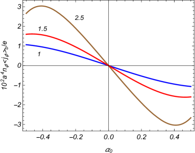
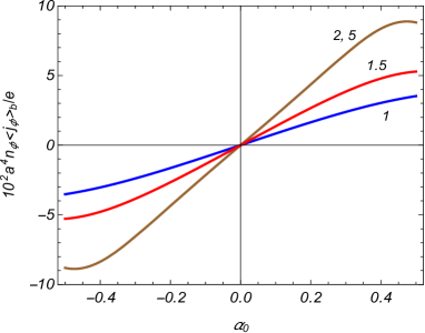
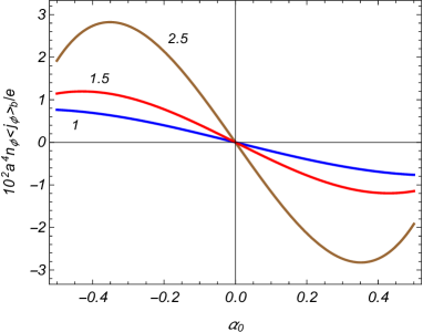
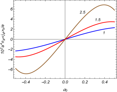
In figures below we plot the charge flux through the hypersurface , given by , measured in units of . The numbers near the curves will correspond to the values of the parameter . Figure 2 presents the corresponding brane-induced contribution in the R-region versus the parameter that determines the fractional part of the ratio of the magnetic flux to flux quantum. The left and right panels correspond to fermionic fields with and , respectively. The graphs are plotted for , , . As seen, the absolute value of the current density increases with increasing planar angle deficit. As it has been already mentioned, for it is a linear function of the parameter . We also see that the absolute value of the brane-induced current density for the case is significantly larger compared to that for the field with .
 |
|
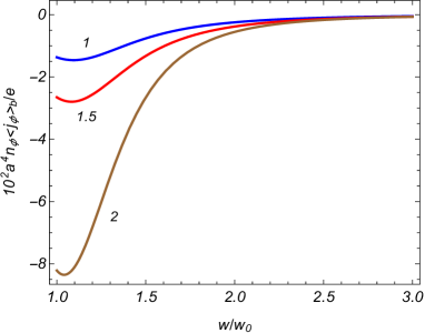
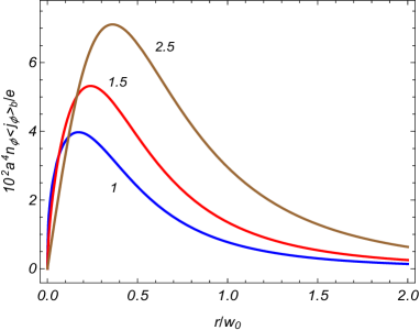
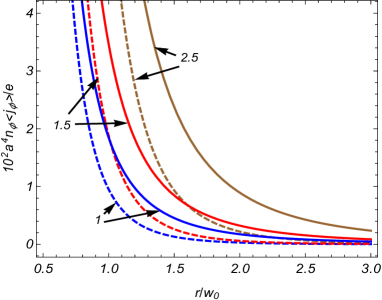
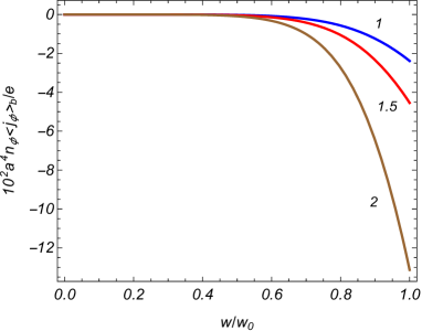
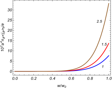
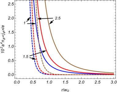
In figure 3 we display the dependence of the brane-induced current density on the ratio for fields with (left panel) and (right panel). For the parameters we have taken , , . Note that the proper distance from the brane is expressed as . As it has been shown by the asymptotic analysis, for the brane-induced contribution decays as . The decay is stronger for the field with .
 |
|
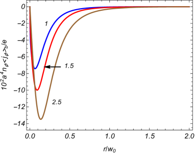
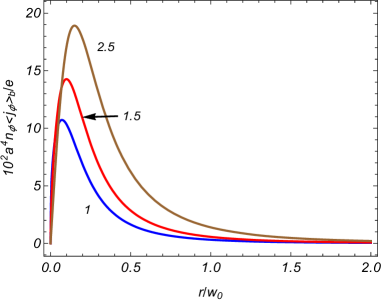
The dependence of the brane-induced current density on the distance from the string is plotted in figure 4 for fixed values of the combinations , , . As before the left and right panels correspond to and . The contribution of the brane linearly vanishes on the string (see (3.34)). At large distances from the string it behaves like . The fall-off is stronger for the case .
 |
|
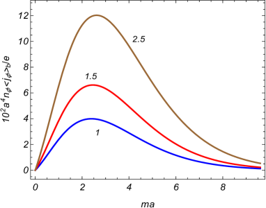
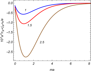
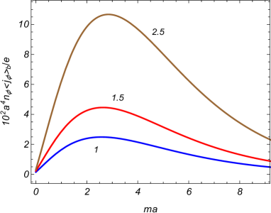
It is of interest to consider the dependence of the current density on the mass of the field. Figure 5 displays that dependence for the brane-induced contribution for , , and for fields with (left panel) and (right panel). As it has been mentioned above, the brane-induced VEV in the R-region vanishes for a massless field. We also expect that for large masses the VEV should tend to zero and, hence, for some intermediate value of the mass the absolute value of the current density has a maximum. That is seen from the graphs.
 |
|
In the numerical examples above we have considered the brane-induced part in the current density. To show its relative contribution, in figure 6 the total current density in the R-region is plotted versus the distance from the string for fixed values , , . For these values the brane-free contribution is positive and monotonically decays with increasing . For the field with (dashed curves), though the brane-induced part is negative, the brane-free contribution dominates at all distances and the total current density is positive. For the field with (full curves) both contributions are positive. For , the total current density near the string is dominated by the brane-free part and at large distances the brane-induced part dominates.
4 Vacuum current in the L-region
In this section we consider the VEV of the current density in the region between the AdS boundary and the brane, corresponding to .
4.1 Integral representation
The complete set of fermionic modes has the form (2.8) with the function given by (2.11). Now, in the normalization condition (2.14) the integration goes over the region . For and the normalization integral diverges at the lower limit and the corresponding mode functions are not normalizable. Hence, in this case the normalizability condition implies that and (the constant is included in the normalization coefficient). For the modes with are normalizable and an additional boundary condition on the AdS boundary is required to uniquely define the wave-functions. Here we will assume a special boundary condition corresponding to . Hence, in our consideration the fermionic mode functions are given by (2.8) with for .
From the boundary condition (2.3) it follows that the eigenvalues for the quantum number are roots of the equation
| (4.1) |
for both the cases . We will denote the corresponding positive roots with respect to by , with , assuming that they are enumerated in the ascending order, . Note that the roots do not depend on the location of the brane. Substituting the mode functions in (2.14) and using the corresponding standard integral involving the products of the Bessel functions, for the normalization constants in the L-region, , we get
| (4.2) |
where the energy is given by . As seen, the normalization coefficients are independent of the representation adopted, or .
Having specified the complete set of modes we can start the investigation of the current density by using the formula (2.7). Similar to the R-region, it can be seen that the only nonzero component corresponds to the one along the azimuthal direction. After the summation over , we get
| (4.3) | |||||
By using the integral representation (3.7) and making transformations similar to those we have described in the previous section for the R-region, the following expression is obtained
| (4.4) | |||||
where .
In order to obtain a representation more convenient for the asymptotic and numerical analysis, and for explicit extraction of the brane-induced contribution, we apply to the series over a variant of the generalized Abel-Plana formula [64],
| (4.5) | |||||
valid for a function analytic in the right half-plane of the complex variable (function may have branch points on the imaginary axis, for the conditions imposed on this function see [64]). For the problem under consideration the function is specified as
| (4.6) |
with . For this function one has
| (4.7) |
The contribution to the current density coming from the first term in the right-hand side of (4.5) coincides with the current density in the geometry without the brane given by (3.16). As a result, the current density in the L-region is decomposed as (3.17), where the brane-induced contribution, coming from the last term in (4.5), is presented as
| (4.8) | |||||
It is an odd periodic function of the magnetic flux with the period of the flux quantum.
Comparing with (3.20), we see that the brane-induced contribution in the L-region is obtained from the corresponding quantity for the R-region by the replacements , of the modified Bessel functions and the replacements of the orders. The expression for the brane-induced contribution in the L-region at half-integer values of the ratio of the magnetic flux to flux quantum is obtained from (3.23) by the same replacements. The limiting values are linear functions of the parameter describing the planar angle deficit. Another special case with corresponds to magnetic flux tube in AdS spacetime. The corresponding expression reads
| (4.9) | |||||
For a massless field one has and . Expanding and evaluating the integral over by using the result from [58], from (4.8) we find
| (4.10) | |||||
Massless fermionic field is conformally invariant and the expression (4.10) is conformally related to the corresponding result in the Minkowski bulk: . Here, is the boundary-induced current density in the region between two boundaries located at and in (4+1)-dimensional Minkowski spacetime with a cosmic string (the line element is given by the expression in the brackets of (2.1)). The boundary in the Minkowskian problem is the conformal image of the AdS boundary. The vacuum polarization effects induced by planar boundaries orthogonal to cosmic string in the Minkowski bulk have been investigated in [65, 66, 67, 68].
4.2 Asymptotic and numerical analysis
We start the asymptotic analysis considering the points near the string, assuming that . By taking into account that in this region the argument of the Bessel function in (4.8) is small, for the leading order term we find
| (4.11) |
and the brane induced VEV linearly vanishes on the string. At large distances from the string we use the representation (4.4). The dominant contribution comes from the lowest eigenmode for and for the VEV of the current density is suppressed by the exponential factor . For the suppression is stronger, by the factor . Recall that in the R-region the decay of the vacuum current at large distances from the string is power-law for both massless and massive fields.
For points close to the AdS boundary, , the dominant contribution in the integral over given in (4.8) comes from the region of integration where the argument of the functions is small. By using the corresponding asymptotic expression [59], to the leading order one has
| (4.12) | |||||
As we observe, the brane-induced current on the AdS boundary vanishes as . Note that this suppression factor does not depend on the parameter . The expression in the right-hand side of (4.12) also describes the behavior of the current in the limit when the location of the brane is close to the AdS horizon for fixed . If in addition , that expression is further simplified as
| (4.13) |
For the evaluation of the current density on the brane it is more convenient to use the representation (4.4) directly putting :
| (4.14) | |||||
The consideration of the Minkowskian limit is similar to that of the R-region. The corresponding result is given by (3.42) with replaced by . Of course, in the Minkowskian limit the VEV is symmetric with respect to the brane. For the AdS bulk, though the local geometrical characteristics are the same in the R- and L-regions, the extrinsic curvature tensor, , for the brane under consideration is different for those regions ( in the R-region and in the L-region). As a consequence, the physical properties of the vacuum state, in particular, the current densities, differ in those regions. The limiting values of the current densities on the brane are different for the R- and L-regions. The discontinuity is related to the idealized model for the brane with zero thickness that constraints all the modes of the vacuum fluctuations. This idealization leads, for example, to surface divergences in the fermion condensate and in the VEV of the energy-momentum tensor. In more realistic models, the fluctuations with high frequencies are relatively insensitive to the presence of the brane. We expect that the formulas for the current density given above will correctly approximate the corresponding results in more realistic models for distances from the brane larger than the cutoff wavelength. The latter is determined by the specific model for the brane.
Now we turn to the results of numerical investigations for the current density in the L-region. As before, the numbers near the curves present the values of the parameter . The left and right panels in figures correspond to fields with and , respectively. In figure 7 the brane-induced current density is plotted as a function of for , , . For these values of the parameters the absolute value of the current density increases with increasing . However, this is not a general feature. For points too close to the string we have an opposite behavior (see figure 9 below).
 |
|
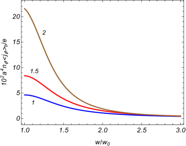
Figure 8 displays the dependence of the current density on the ratio for fixed , , . As it has been already shown by the asymptotic analysis, the current density tends to zero on the AdS boundary like for both cases and .
 |
|
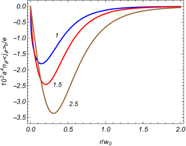
The brane-induced current density versus the distance from the string is depicted in figure 9 for , , . Recall that in the L-region the suppression of the current density at large distances from the string is stronger compared to the behavior in the R-region. One has an exponential decay insted of power-law fall-off for the R-region.
 |
|
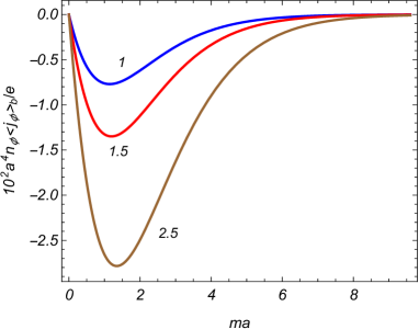
Figure 10 presents the brane-induced current density as a function of the mass for the values , , . Unlike the R-region, the current density for massless fields does not vanish. In the case (left panel), the corresponding values of the combination , plotted in figure 10, are equal for , respectively. For the field (right panel) the respective values are given by . Again, we see that the current density is not a monotonic function of the mass. At some intermediate value of the mass its absolute value takes the maximum. For the example given in figure 10 the absolute value of the current density at the maximum is essentially larger compared to the current density for a massless field.
 |
|
Finally, in figure 11 we plot the total current density versus the distance from the string for , , . Full and dashed curves correspond to the fields with and , respectively. Similar to the R-region, at large distances from the string the current density for the first case is dominated by the brane-induced contribution.
5 Vacuum current for the second type of boundary condition
In this section we consider the brane-induced contribution to the VEV of the azimuthal current density for the boundary condition
| (5.1) |
The latter differs from (2.3) by the sign of the term containing the Dirac matrices. As it will be seen below both the boundary conditions (2.3) and (5.1) appear in Randall-Sundrum type models as a consequence of the -symmetry with respect to the brane. The evaluation procedure for the condition (5.1) is similar to that we have described in the previous sections and the final results will be presented only.
5.1 R-region
We start with the R-region. The corresponding mode functions are given by (2.8) where now
| (5.2) |
The expression for the normalization coefficient is obtained from (3.3) by the replacement in the orders of the Bessel and Neumann functions. The mode-sum for the VEV of the azimuthal current density is expressed as
| (5.3) | |||||
with . It is decomposed as (3.17) with the brane-induced contribution
| (5.4) | |||||
Now comparing these formulas with (3.5) and (3.20), we see that the VEVs of the current density for and for the boundary condition (5.1) coincide with the VEVs for the boundary condition (2.3) and for .
5.2 L-region
In the L-region the mode functions for the boundary condition (5.1) are given by (2.8) with . The eigenvalues of the quantum number are determined from the boundary condition and are roots of the equation . The normalization coefficient is given by (4.2) with the replacement in the order of the Bessel function. For the VEV of the azimuthal current density one gets
| (5.5) | |||||
In a way similar to that we have used in section 4, by using the summation formula that is obtained from (4.5) by the replacements , , for the brane-induced contribution in the L-region we find
| (5.6) | |||||
For a given , the VEV of the azimuthal current density for the boundary condition (5.1) coincides with that for the condition (2.3) and for replaced by .
6 Current density in - and -symmetric models
In odd-dimensional spacetimes the Clifford algebra has two inequivalent irreducible representations. For the spatial dimension we consider here, the corresponding sets of the flat spacetime gamma matrices can be taken in the form , where specify the representations and the matrices are obtained from the corresponding matrices in (2.4) omitting the factors . Note that one has the relation . We introduce fermionic fields corresponding to a given representation and having the Lagrangian , where are the curved spacetime gamma matrices and is the respective spin connection. Note that, as it follows from (2.6), the product is the same for and . For massive fields, the separate Lagrangians with a given are not invariant under the charge conjugation () and parity transformation (). The models invariant under these transformations in the absence of external gauge field can be constructed considering the set of two fields with and and with the Lagrangian . In these models the VEV of the total current density, , is the sum of the VEVs corresponding to the separate fields: , where . Note that the matrices coincide with those we have used in the previous sections.
Let us pass to a new set of fields by the transformations , . By taking into account that and , the total Lagrangian is presented in the form . For the fields the Dirac equation is reduced to (2.2). This shows that the parameter in the previous discussion corresponds to different representations of the Clifford algebra. For the current densities of the separate fields we get .
Now let us turn to the boundary conditions on the brane. First we consider the case when both the fields obey the boundary condition (2.3):
| (6.1) |
In terms of the new fields these conditions take the form
| (6.2) |
We see that the field obeys the field equation and the boundary condition discussed in sections 3 and 4 for the case . Hence, the brane-induced contributions in the corresponding current densities in the R- and L-regions are given by (3.20) and (4.8) with and . The field obeys the field equation (2.2) with and the boundary condition (5.1). As it has been discussed in the previous section, the corresponding VEVs of the current density in the R- and L-regions coincide with those considered in sections 3 and 4 for the case and for the condition (2.3). Hence, we conclude that in the case of the boundary conditions (6.1) the current densities coincide for the fields corresponding to the representations and . The total current density is obtained from the expressions given in sections 3 and 4 with and with an additional factor 2.
From (6.2) we see that the boundary conditions for the fields and differ by the sign of the terms with the Dirac matrices. We can consider the case where those terms have the same sign and the transformed fields obey the same boundary condition . That corresponds to the conditions for the initial fields on the brane . With these boundary conditions, the current density for the field with remains the same as that for (6.1) and is given by the expressions in sections 3 and 4 with . However, now the VEV is different. It is given by the expressions from sections 3 and 4 with . In this case the fields realizing two inequivalent irreducible representations of the Clifford algebra give different contributions to the brane-induced part in the VEV of the total current density.
7 Applications to Randall-Sundrum model
The results given above can be directly applied for the investigation of the cosmic string induced effects in background of the Randall-Sundrum model with a single brane (RSII model) [69, 70] (for quantum effects in higher-dimensional generalizations of RSII model see [71] and references therein). In the presence of cosmic string perpendicular to the brane, the corresponding background geometry contains two copies of the R-region that are identified by the -symmetry with respect to the brane located at (or at in terms of the coordinate ). The corresponding line element is expressed as
| (7.1) |
where, as before, and . Note that for an observer located on the brane the line element (7.1) is reduced to the standard line element for a cosmic string in (3+1)-dimensional Minkowski spacetime. The boundary condition for the field on the brane is obtained on the basis of the -symmetry (see discussion in [51, 72]).
Let be the matrix that relates the fields in the regions and :
| (7.2) |
We require the invariance of the fermionic field action under the identification of the points in those region. This requirement leads to the following conditions on the matrix :
| (7.3) |
where . By direct substitution it can be checked that these relations are obeyed by the matrix with a constant . For the latter from the relation we find and the transformation matrix has the form
| (7.4) |
Hence, we have two types of fermionic fields with the identification rule (7.2) and with the upper and lower signs in (7.4).
On the brane at one gets the following boundary condition
| (7.5) |
Now we can see that the boundary condition (7.5) with the upper sign in (7.4) coincides with the condition (2.3) and the boundary condition (7.5) with the lower sign coincides with the condition (5.1). Hence, for the fermionic field corresponding to the upper sign in (7.4), the expressions for the VEV of the current density induced by a cosmic string in the RSII model is obtained from the formulas in section 3 taking and adding an additional factor 1/2. For the field with the lower sign in (7.4) the corresponding result is obtained from the expression for the current density in section 5.1 for the R-region (again, with a factor 1/2). The appearance of the factor 1/2 is related to that the integration in the normalization condition for the mode functions goes over the interval instead of the interval for the R-region in the discussion above (with ).
The current density induced on the brane by vacuum fluctuations of a bulk fermionic field is a source of magnetic fields surrounding the cosmic string. These fields are among the distinctive features of magnetic-flux-carrying strings. Note that the vacuum current density will also be generated by quantum fluctuations of fields living on the brane (for example, Standard Model fields in braneworld scenario). However, the corresponding properties are different from those we have discussed above (for fermionic currents in the geometry of a cosmic string on background of (3+1)-dimensional Minkowski spacetime see [55, 73, 74]). As a consequence, the structure of magnetic fields around the cosmic string is sensitive to the existence of extra dimensions.
8 Conclusion
We have investigated the combined effects of the gravitational filed and a brane on the vacuum current density for a charged fermionic field around a magnetic-flux-carrying cosmic string. In order to have an exactly solvable problem we have considered highly symmetric bulk and boundary geometries, namely, AdS spacetime and a planar brane perpendicular to the cosmic string. Two types of boundary conditions have been discussed on the brane. The first one corresponds to the MIT bag boundary condition and the second one is given by (5.1). The current density for the field realizing the representation and the boundary condition (5.1) coincides with the current density for the representation and for the boundary condition (2.3) and we have described the main steps of the evaluation procedure for the bag boundary condition only. The VEV of the current density is expressed in the form of mode-sum over the complete set of fermionic modes. The latter are given by (2.8). The brane divides the space into two regions (R- and L-regions) with different properties of the fermionic vacuum. In the R-region the function in the mode functions is given by (3.1) and the spectrum of the quantum number is continuous. In the L-region one has and the eigenvalues for are determined by the zeros of the function .
The only nonzero component of the vacuum current density corresponds to the current along the -direction (azimuthal current). It is decomposed into brane-free and brane-induced parts. The brane-induced contributions in the VEV of the azimuthal current density are given by the expressions (3.20) and (4.8) for the R- and L-regions, respectively. For a massless field the brane-induced contribution vanishes in the R-region. The current density is an odd periodic function of the magnetic flux along the string axis, with the period equal the flux quantum. It is discontinuous at half-integer values of the magnetic flux in units of flux quantum. The corresponding limiting values are linear functions of the parameter and are expressed as (3.23). In the special case the formulas obtained provide the expressions for the current densities induced by idealized magnetic flux tubes with zero thickness. In the limit of large values for the curvature radius of the background spacetime, in the leading order we have derived the expression (3.42) for the fermionic current density induced by a planar boundary, perpendicular to cosmic string in -dimensional Minkowski spacetime.
To clarify the behavior of the azimuthal current density we have considered various asymptotic regions of the parameters in the problem. Near the cosmic string, for points not too close to the brane, the brane-induced contribution is a linear function of the radial coordinate and vanishes on the string. Near the string the brane-free part behaves as and it dominates in the total VEV. At large proper distances from the string, compared with the curvature radius of the AdS spacetime, one has and the brane-free VEV decays like . The behavior of the brane-induced contribution in the R-region at large distances from the string is different for the fields realizing two different irreducible representations of the Clifford algebra. For the representation with the total current density at large distances is dominated by the brane-free part. For the representation with the brane-induced contribution behaves as and it is dominant in the total VEV. In all these cases, the decay of the current density on AdS bulk, as a function of the proper distance from the string, is power-law for both massless and massive fields. For massive fields this large-distance asymptotic in the R-region is in clear contrast to that for the Minkowski bulk where the decay is exponential. At large distances from the string the current density in L-region is suppressed by the exponential factor for and by the factor for , with being the lowest eigenvalue for the quantum number .
An important difference of the vacuum current density from the VEV of the energy-momentum tensor is its finiteness on the brane. The corresponding limiting values for the R- and L-region are directly obtained from the representations (3.13), (4.4) and they are given by (3.39) and (4.14). At large distances from the brane, , , the brane-induced current density in the R-region is suppressed by the factor for . The suppression is stronger for the representation . For and the brane-induced current density tends to finite value on the AdS horizon (), determined from (3.38). For a fixed location of the brane and in the limit , corresponding to points on the AdS boundary, the brane-induced VEV behaves like . The same is the case for the brane-free contribution.
In -dimensional spacetime the Lagrangian for a massive fermionic field realizing the irreducible representation of the Clifford algebra is not invariant under charge conjugation and parity transformation. - and -invariant fermionic models are constructed by combining the fields , , corresponding to two inequivalent sets of Dirac matrices . By the transformation of the fields, the model with two fields is reduced to the model with the fields such that the new fields obey the equation (2.2). When the fields obey the same boundary conditions, the boundary conditions for the fields differ by the sign of the term containing the normal to the boundary. In this case the VEVs of the current densities for separate fields coincide. In the second case the boundary conditions are the same for the fields and differ by the sign of the term containing the normal for the fields . In this case the vacuum currents differ and the corresponding expressions are obtained from the formulas given in sections 3 and 4 with and .
In the Randall-Sundrum model with a single brane the boundary conditions on a bulk fermionic field is dictated by the -symmetry. Depending on the parity of the field, two boundary conditions are obtained at the location of the brane. They correspond to the conditions (2.3) and (5.1) in our discussion. Consequently, the VEV of the current density for a bulk fermionic field, induced by magnetic-flux-carrying cosmic string RSII model, is obtained from the results in sections 3 and 4 with an additional factor 1/2, related to the presence of two copies of the R-region.
For the convenience of the reader, in table 1 we summarize the main formulas for the VEV of the azimuthal current density.
| Brane-free part of the current density | (3.16),(3.26) |
|---|---|
| Boundary-free contribution in the Minkowski bulk | (3.33) |
| Boundary-induced contribution in the Minkowski bulk | (3.42) |
| Total current density in the R-region | (3.13) |
| Brane-induced contribution to the current density in the R-region | (3.20) |
| Total current density in the L-region | (4.4) |
| Brane-induced contribution to the current density in the L-region | (4.8) |
| Brane-induced contribution to the current density in the L-region | (4.10) |
| for a massless field |
Acknowledgments
This study was financed in part by the Coordenação de Aperfeiçoamento de Pessoal de Nível Superior - Brasil (CAPES) - Finance Code 001. E.R.B.M is partially supported by CNPq under Grant no 301.783/2019-3.
References
- [1] C. G. Callan, Jr., and F. Wilczek, Nucl. Phys. B340, 366 (1990).
- [2] C. Fronsdal, Phys. Rev. D 10, 589 (1974).
- [3] C. Fronsdal and R. B. Haugen, Phys. Rev. D 12, 3810 (1975).
- [4] S. J. Avis, C. J. Isham and D. Storey, Phys. Rev. D 18, 3565 (1978).
- [5] E. S. Fradkin and A. A. Tseytlin, Nucl. Phys. B234, 472 (1984).
- [6] N. Sakai and Y. Tanii, Phys. Lett. B146, 38 (1984).
- [7] C. Dullemond and E. van Beveren, J. Math. Phys. 26, 2050 (1985).
- [8] C. P. Burgess and C. A. Lütken, Phys. Lett. B153, 137 (1985)
- [9] W. F. Heidenreich, Phys. Rev. D 36, 1685 (1987).
- [10] R. Camporesi, Phys. Rev. D 43, 3958 (1991).
- [11] M. Kamela and C. P. Burgess, Can. J. Phys. 77, 85 (1999)
- [12] W. D. Goldberger and I. Z. Rothstein, Phys. Rev. Lett. 89, 131601 (2002).
- [13] A. Das and G. V. Dunne, Phys. Rev. D 74, 044029 (2006).
- [14] O. Aharony, D. Marolf and M. Rangamani, JHEP 02(2011)041.
- [15] O. Aharony, M. Berkooz, D. Tong and S. Yankielowicz, JHEP 02(2013)076.
- [16] I. Fujisawa and R. Nakayama, Nucl. Phys. B 886, 135 (2014).
- [17] V. E. Ambruş and E. Winstanley, Phys. Lett. B 749, 597 (2015).
- [18] C. Kent and E. Winstanley, Phys. Rev. D 91, 044044 (2015).
- [19] A. Belokogne, A. Folacci and J. Queva, Phys. Rev. D 94, 105028 (2016).
- [20] V. E. Ambruş and E. Winstanley, Class. Quantum Grav. 34, 145010 (2017).
- [21] V. E. Ambruş, C. Kent and E. Winstanley, Int. J. Mod. Phys. D 27, 1843014 (2018).
- [22] C. Dappiaggi, H. Ferreira and A. Marta, Phys. Rev. D 98, 025005 (2018).
- [23] T. Morley, P. Taylor and E. Winstanley, Quantum field theory on global anti-de Sitter space-time with Robin boundary conditions, arXiv:2004.02704.
- [24] T. W. Kibble, J. Phys. A 9, 1387 (1976).
- [25] A. Vilenkin and E. P. S. Shellard, Cosmic Strings and Other Topological Defects (Cambridge University Press, Cambridge, England, 1994).
- [26] M. B. Hindmarsh and T. W. B. Kibble, Rep. Prog. Phys. 58, 477 (1995).
- [27] E. Witten, Phys. Lett. B 153, 243 (1985).
- [28] G. Dvali and S. H. Henry Tye, Phys. Lett. B 450, 72 (1999).
- [29] S. H. Henry Tye, Lect. Notes Phys. 737, 949 (2008).
- [30] E. J. Copeland and T. W. B. Kibble, Proc. R. Soc. A 466, 623 (2010).
- [31] E. J. Copeland, L. Pogosian and T.Vachaspati, Class. Quantum Grav. 28, 204009 (2011)
- [32] D. F. Chernoff and S. H. Henry Tye, Int. J. Mod. Phys. D 24, 1530010 (2015).
- [33] S. Sarangi and S. H. Henry Tye, Phys. Lett. B 536, 185 (2002).
- [34] S. C. Davis, Phys. Lett. B 499, 179 (2001).
- [35] S. C. Davis, Phys. Lett. B 645, 323 (2007).
- [36] M. Heydari-Fard, H. Razmi and S. Y. Rokni, Class. Quantum Grav. 30, 165001 (2013).
- [37] N. R. F. Braga and C. N. Ferreira, J. High Energy Phys. 03 (2005) 039.
- [38] M. C. B. Abdalla, M. E. X. Guimarães and J. M. H. da Silva, Phys. Rev. D 75, 084028 (2007).
- [39] M. C. B. Abdalla, P. F. Carlesso and J. M. Hoff da Silva, , Eur. Phys. J. Plus 75, 432 (2015).
- [40] M. H. Dehghani, A. M. Ghezelbash and R. B. Mann, Nucl. Phys. B 625, 389 (2002).
- [41] C. A. Ballon Bayona, C. N. Ferreira and V. J. Vasquez Otoya, Class. Quantum Grav. 28, 015011 (2011).
- [42] E. R. Bezerra de Mello and A. A. Saharian, J. Phys. A 45 115402 (2012).
- [43] E. R. Bezerra de Mello, E. R. Figueiredo Medeiros and A. A. Saharian, Class. Quantum Grav. 30, 175001 (2013).
- [44] W. Oliveira dos Santos, H. F. Mota and E. R. Bezerra de Mello, Phys. Rev. D 99, 045005 (2019).
- [45] W. Oliveira dos Santos, E. R. Bezerra de Mello and H. F. Mota, Eur. Phys. J. Plus 135, 27 (2020).
- [46] S. Bellucci, W. Oliveira dos Santos and E. R. Bezerra de Mello, Eur. Phys. J. C 80, 963 (2020).
- [47] E. R. Bezerra de Mello, A. A. Saharian and V. Vardanyan, Phys. Lett. B 741, 155 (2015).
- [48] S. Bellucci, A. A. Saharian and V. Vardanyan, JHEP 11(2015)092.
- [49] S. Bellucci, A. A. Saharian and V. Vardanyan, Phys. Rev. D 93, 084011 (2016).
- [50] S. Bellucci, A. A. Saharian and V. Vardanyan, Phys. Rev. D 96, 065025 (2017).
- [51] S. Bellucci, A. A. Saharian, D. H. Simonyan and V. Vardanyan, Phys. Rev. D 98, 085020 (2018).
- [52] S. Bellucci, A. A. Saharian, H. G. Sargsyan and V. Vardanyan, Phys. Rev. D 101, 045020 (2020).
- [53] M. Bordag and N. Khusnutdinov, Class. Quantum Grav. 13, L41 (1996).
- [54] E. R. Bezerra de Mello and A. A. Saharian, Eur. Phys. J. C 73 2532 (2013).
- [55] A. Mohammadi, E. R. Bezerra de Mello and A. A. Saharian, J. Phys. A: Math. Theor. 48, 185401 (2015).
- [56] E. R. Bezerra de Mello, V. B. Bezerra, A. A. Saharian and H. H. Harutyunyan, Phys. Rev. D 91, 064034 (2015).
- [57] E. R. Bezerra de Mello, V. B. Bezerra, A.A. Saharian and V.M. Bardeghyan, Phys. Rev. D 82, 085033 (2010).
- [58] A. P. Prudnikov, Yu. A. Brychkov and O. I. Marichev, Integrals and Series (Gordon and Breach, New York, 1986), Vol. 2.
- [59] Handbook of Mathematical Functions, edited by M. Abramowitz and I. A. Stegun (Dover, New York, 1972).
- [60] S. Bellucci, E. R. Bezerra de Mello, E. Braganca and A. A. Saharian, Eur. Phys. J. C 76, 350 (2016).
- [61] A. A. Saharian, E. R. Bezerra de Mello and A. A. Saharyan, Phys. Rev. D 100, 105014 (2019).
- [62] S. Bellucci, I. Brevik, A. A. Saharian and H. G. Sargsyan, Eur. Phys. J. C 80, 281 (2020).
- [63] S. Bellucci, A. A. Saharian and A. Kh. Grigoryan, Phys. Rev. D 94, 105007 (2016).
- [64] A. A. Saharian, The generalized Abel-Plana formula with applications to Bessel functions and Casimir effect, arXiv:0708.1187 [hep-th].
- [65] E. R. Bezerra de Mello and A. A. Saharian, Class. Quantum Grav. 28, 145008 (2011).
- [66] E. R. Bezerra de Mello, A. A. Saharian and A. Kh. Grigoryan, J. Phys. A: Math. Theor. 45, 374011 (2012).
- [67] E. R. Bezerra de Mello, A. A. Saharian and S. V. Abajyan, Class. Quantum Grav. 30, 015002 (2013).
- [68] E. R. Bezerra de Mello, A. A. Saharian and S. V. Abajyan, Phys. Rev. D 97, 085023 (2018).
- [69] L. Randall and R. Sundrum, Phys. Rev. Lett. 83, 3370 (1999).
- [70] L. Randall and R. Sundrum, Phys. Rev. Lett. 83, 4690 (1999).
- [71] A. A. Saharian, Universe 6, 181 (2020).
- [72] A. Flachi, I.G. Moss and D.J. Toms, Phys. Rev. D 64, 105029 (2001).
- [73] E. R. Bezerra de Mello, Class. Quantum Grav. 27, 095017 (2010).
- [74] E. R. Bezerra de Mello and A. A. Saharian, Eur. Phys. J. C 73, 2532 (2013).