Learning Discrete Energy-based Models via
Auxiliary-variable Local Exploration

Abstract

Discrete structures play an important role in applications like program language modeling and software engineering. Current approaches to predicting complex structures typically consider autoregressive models for their tractability, with some sacrifice in flexibility. Energy-based models (EBMs) on the other hand offer a more flexible and thus more powerful approach to modeling such distributions, but require partition function estimation. In this paper we propose ALOE, a new algorithm for learning conditional and unconditional EBMs for discrete structured data, where parameter gradients are estimated using a learned sampler that mimics local search. We show that the energy function and sampler can be trained efficiently via a new variational form of power iteration, achieving a better trade-off between flexibility and tractability. Experimentally, we show that learning local search leads to significant improvements in challenging application domains. Most notably, we present an energy model guided fuzzer for software testing that achieves comparable performance to well engineered fuzzing engines like libfuzzer.

1 Introduction

Many real-world applications involve prediction of discrete structured data, such as syntax trees for natural language processing [1, 2], sequences of source code tokens for program synthesis [3], and structured test inputs for software testing [4]. A common approach for modeling a distribution over structured data is the autoregressive model. Although any distribution can be factorized in such a way, the parameter sharing used in neural autoregressive models can restrict their flexibility. Intuitively, a standard way to perform inference with autoregressive models has a single pass with a predetermined order, which forces commitment to early decisions that cannot subsequently be rectified. Energy-based models [5] (EBMs), on the other hand, define the distribution with an unnormalized energy function, which allows greater flexibility by not committing to any inference order. In principle, this allows more flexible model parameterizations such as bi-directional LSTMs, tree LSTMs [1, 2], and graph neural networks [6, 7] to be used to capture non-local dependencies.

Unfortunately, the flexibility of EBMs exacerbates the difficulties of learning and inference, since the partition function is typically intractable. EBM learning algorithms therefore employ approximate strategies such as contrastive learning, where positive samples are drawn from data and negative samples obtained from an alternative sampler [8]. Contrastive divergence [9, 10, 11, 12], pseudo-likelihood [13] and score matching [14] are all examples of such a strategy. However, such approaches use hand-designed negative samplers, which can be overly restrictive in practice, thus [8, 15, 16] consider joint training of a flexible negative sampler along with the energy function, achieving significant improvements in model quality. These recent techniques are not directly applicable to discrete structured data however, since they exploit gradients over the data space. In addition, the parameter gradient involves an intractable sum, which also poses a well-known challenge for stochastic estimation [17, 18, 19, 20, 21, 22, 23, 24].

In this work, we propose Auxiliary-variable LOcal Exploration (ALOE), a new method for discrete EBM training with a learned negative sampler. Inspired by viewing MCMC as a local search in continuous space, we parameterize the learned sampler using local discrete search; that is, the sampler first generates an initial negative structure using a tractable model, such as an autoregressive model, then repeatedly makes local changes to the structure. This provides a learnable negative sampler that still depends globally on the sequence. As there are no demonstrations for intermediate steps in the local search, we treat it as an auxiliary variable model. To learn this negative sampler, instead of the primal-dual form of MLE [25, 8], we propose a new variational objective that uses finite-step MCMC sampling for the gradient estimator, resulting in an efficient method. The procedure alternates between updating the energy function and improving the dual sampler by power iteration, which can be understood as generalization of persistent contrastive divergence (PCD [10]).

We experimentally evaluated the approach on both synthetic and real-world tasks. For a program synthesis problem, we observe significant accuracy improvements over the baseline methods. More notably, for a software testing task, a fuzz test guided by an EBM achieves comparable performance to a well-engineered fuzzing engine on several open source software projects.

2 Preliminaries

Energy-based Models: Let $x\in\mathcal{S}$ be a discrete structured datum in the space $\mathcal{S}$. We are interested in learning an energy function $f:\mathcal{S}\rightarrow\mathbb{R}$ that characterizes the distribution on $\mathcal{S}$. Depending on the space, $f$ can be realized as an LSTM [26] for sequence data, a tree LSTM [1] for tree structures, or a graph neural network [6] for graphs. The probability density function is defined as

$$p_{f}(x)=\exp\left(f(x)-\log Z_{f}\right)\propto\exp\left(f(x)\right),$$ (1)

where $Z_{f}:=\sum_{x\in\mathcal{S}}\exp\left(f(x)\right)$ is the partition function.

It is natural to extend the above model for conditional distributions. Let $z\in\mathcal{Z}$ be an arbitrary datum in the space $\mathcal{Z}$. Then a conditional model is given by the density

$$p_{f}(x|z)=\frac{\exp\left(f(x,z)\right)}{Z_{f,z}},\text{ where }Z_{f,z}=\sum_{x\in\mathcal{S}}\exp\left(f(x,z)\right).$$ (2)

Typically $\mathcal{S}$ is a combinatorial set, which makes the partition function $Z_{f}$ or $Z_{f,z}$ intractable to calculate. This makes both learning and inference difficult.

Primal-Dual view of MLE: Let $\mathcal{D}=\left\{x_{i}\right\}_{i=1}^{|\mathcal{D}|}$ be a sample obtained from some unknown distribution over $\mathcal{S}$. We consider maximizing the log likelihood of $\mathcal{D}$ under model $p_{f}$:

$$\max_{f}\,\,\ell\left(f\right):=\mathbb{E}_{x\sim\mathcal{D}}\left[f(x)\right]-\log Z_{f}.$$ (3)

Directly maximizing this objective is not feasible due to the intractable log partition term. Previous work [15, 8] reformulates the MLE by exploiting the Fenchel duality of the $\log$-partition function, i.e., $\log Z_{f}=\max_{q}\mathbb{E}_{x\sim q}\left[f(x)\right]-H(q)$, where $H(q)=-\mathbb{E}_{q}\left[\log q\right]$ is the entropy of $q\left(\cdot\right)$, which leads to a primal-dual view of the MLE:

$$\max_{f}\min_{q}\,\,\bar{\ell}\left(f,q\right):=\underbrace{\mathbb{E}_{x\sim\mathcal{D}}\left[f(x)\right]}_{\text{positive sampling}}-\underbrace{\mathbb{E}_{x\sim q}\left[f(x)\right]}_{\text{negative sampling}}-H(q)$$ (4)

Although the primal-dual view introduces an extra dual distribution $q\left(x\right)$ for negative sampling, this provides an opportunity to use a trainable deep neural network to capture the intrinsic data manifold, which can lead to a better negative sampler. In [8], a family of flexible negative samplers was introduced, which combines learnable components with dynamics-based MCMC samplers, e.g., Hamiltonian Monte Carlo (HMC) [27] and stochastic gradient Langevin dynamics (SGLD) [28], to obtain significant practical improvements in continuous data modeling. However, the success of this approach relied on the differentiability of $q$ and $f$ over a continuous domain, requiring guidance not only from $\nabla_{x}f\left(x\right)$, but also from gradient back-propagation through samples, i.e., $\nabla_{\phi}\bar{\ell}\left(f,q\right)=-\nabla_{\phi}\mathbb{E}_{x\sim q_{\phi}}\left[\nabla_{x}f\left(x\right)\nabla_{\phi}x\right]$ where $\phi$ denotes the parameters of the dual distribution. Unfortunately, for discrete data, learning a dual distribution for negative sampling is difficult. Therefore this approach is not directly translatable to discrete EBMs.

3 Auxiliary-variable Local Exploration

To extend the above approach to discrete domains, we first introduce a variational form of power iteration (Section 3.1) combined with local search (Section 3.2). We present the method for an unconditional EBM, but the extension to a conditional EBM is straightforward.

3.1 MLE via Variational Gradient Approximation

For discrete data, learning the dual sampler in the min-max form of MLE (4) is notoriously difficult, usually leading to inefficient gradient estimation [17, 18, 19, 20, 21, 22, 23, 24]. Instead we consider an alternative optimization that has the same solution but is computationally preferable:

$$\max_{f,q}\,\,\tilde{\ell}\left(f,q\right):=\max_{f}\max_{q\in\mathcal{K}}\>{\mathbb{E}_{x\sim\mathcal{D}}\left[f\left(x\right)\right]-\mathbb{E}_{x\sim q}\left[f\left(x\right)\right]},$$ (5)

$$\mathcal{K}:=\left\{q\>\middle|\>\int q\left(x\right)k_{f}\left(x^{\prime}|x\right)dx=q\left(x^{\prime}\right),\forall x^{\prime}\in{\mathcal{S}}\right\},$$ (6)

where $k_{f}\left(x^{\prime}|x\right)$ is any ergodic MCMC kernel whose stationary distribution is $p_{f}$.

Theorem 1

Let $\left(f^{*},q^{*}\right)=\mathop{\mathrm{argmax}}_{f,q}\tilde{\ell}\left(f,q\right)$. If the kernel $k_{f}\left(x^{\prime}|x\right)$ is ergodic with stationary distribution $p_{f}$, then $f^{*}=\mathop{\mathrm{argmax}}\ell\left(f\right)$ is the MLE and $q^{*}=p_{f^{*}}$.

Proof  By the ergodicity of $k_{f}\left(x^{\prime}|x\right)$, there is unique feasible solution satisifying the constraint $\int q\left(x\right)k_{f}\left(x^{\prime}|x\right)dx=q\left(x^{\prime}\right)$, which is $p_{f}\left(x\right)$. Substituting this into the gradient of $\tilde{\ell}$ yields

$$\mathbb{E}_{x\sim\mathcal{D}}\left[\nabla_{f}f\left(x\right)\right]-\mathbb{E}_{x\sim q_{f}}\left[\nabla_{f}f\left(x\right)\right]=0,$$

verifying that $f$ is the optimizer of (3).  

Solving the optimization (5) is still nontrivial, as the constraints are in the function space. We therefore propose an alternating update based on the variational form (5):

• Update $q$ by power iteration: Noticing that the constraint actually seeks an eigenfunction of $k_{f}\left(x^{\prime}|x\right)$, we can apply power iteration to find the optimal $q$. Conceptually, this power iteration executes $q_{t+1}(x^{\prime})=\int q_{t}(x)k_{f}\left(x^{\prime}|x\right)dx$ until convergence. However, since the integral is intractable, we instead apply a variational formulation to minimize

  $$q_{t+1}=\mathop{\mathrm{argmin}}_{q}D_{KL}\left(\int q_{t}(x)k_{f}\left(x^{\prime}|x\right)dx\Big{|}\Big{|}q\right)=\mathop{\mathrm{argmin}}_{q}\mathbb{E}_{q_{t}\left(x\right)k_{f}\left(x^{\prime}|x\right)}\left[\log q\left(x^{\prime}\right)\right].$$ (7)

  In practice, this only requires a few power iteration steps. Also we do not need to worry about differentiability with respect to $x$, as (7) needs to be differentiated only with respect to the parameters of $q.$ We will show in the next section that this framework actually allows a much more flexible $q$ than autoregressive, such as a local search algorithm.

• Update $f$ with MLE gradient: Denote $q_{f}^{*}=\mathop{\mathrm{argmax}}_{q\in\mathcal{K}}\tilde{\ell}\left(f,q\right)$. Then $q^{*}_{f}$ converges to $p_{f}$. Recall the unbiased gradient estimator for MLE $\ell\left(f\right)$ w.r.t. $f$ is

  $$\nabla_{f}\ell\left(f\right)=\mathbb{E}_{x\sim\mathcal{D}}\left[\nabla_{f}f\left(x\right)\right]-\mathbb{E}_{x\sim q^{*}_{f}}\left[\nabla_{f}f\left(x\right)\right],$$

By alternating these two updates, we obtain the ALOE framework illustrated in Algorithm 1.

Connection to PCD: When we set the number of power iteration steps to be $1$, the variational form of MLE optimization can be understood as a function generalized version of Persistent Contrastive Divergence (PCD) [10], where we distill the past MCMC samples into the sampler $q$ [29]. Intuitively, since $f$ is optimized by gradient descent, the energy models between adjacent stochastic gradient iterations should still be close, and the power iteration will converge very fast.

Connection to wake-sleep algorithm: ALOE is also closely related to the “wake-sleep” algorithm [30] introduced for learning Helmholtz machines [31]. The “sleep” phase learns the recognition network with objective $D_{KL}(p_{f}||q)$, requiring samples from the current model. However it is hard to obtain such samples for general EBMs, so we exploit power iteration in a variational form.

3.2 Negative sampler as local search with auxiliary variables

Algorithm 1 Main algorithm of ALOE

1:  Input: Observations $\mathcal{D}=\left\{x_{i}\right\}_{i=1}^{|\mathcal{D}|}$

2:  Initialize score function $f$, sampler $q$.

3:  for $x\sim\mathcal{D}$ do

4:     Sample $(\hat{x},\tilde{x})$ from $q(\hat{x})k_{f}(\tilde{x}|\hat{x})$

5:     Update $f$ with $-\nabla_{f}f(x)+\nabla_{f}f(\tilde{x})$

6:     Update $q$ using Algorithm 2

7:  end for

Algorithm 2 Update sampler $q$

1:  Input: Current model $f$

2:  for $i\leftarrow 1$ to # power iteration steps do

3:     Sample $\tilde{x}$ from $q$, and get $x$ from $k_{f}(\cdot|\tilde{x})$.

4:     Sample trajectories $\textstyle\{\mathbf{x}^{j}_{0:t^{j}}\}_{j=1}^{N}$ for $x$ using Eq (13) or Eq (14).

5:     Update $q$ with gradient from Eq (12).

6:  end for

Figure 1: ALOE for learning unconditional discrete EBMs. Algorithms are similar for conditional case. We demonstrate with a single example, but in practice batched optimization is used.

Ideally the sampler $q*$ should converge to the stationary distribution $p_{f}$, which requires a sufficiently flexible distribution. One possible choice for a discrete structure sampler is an autoregressive model, like RobustFill for generating program trees [3] or GGNN for generating graphs [32]. However, these have limited flexibility due to parameters being shared at each decision step, which is needed to handle variable sized structures. Also the “one-pass” inference according to a predefined order makes the initial decisions too important in the entire sampling procedure.

Intuitively, humans do not generate structures sequentially, but perform successive refinement. Recent approaches for continuous EBMs have found that using HMC or SGLD provides more effective learning  [8, 12] by exploiting gradient information. For discrete data, an analogy to gradient based search is local search. In discrete local search, an initial solution can be obtained using a simple algorithm, then local modification can be made to successively improve the structure.

By parameterizing $q$ as a local search algorithm, we obtain a strictly more flexible sampler than the autoregressive counterpart. Specifically, we first generate an initial sample $x_{0}\sim q_{0}$, where $q_{0}$ can be an autoregressive distribution with parameter sharing, or even a fully factorized distribution. Next we obtain a new sample using an editor $q_{A}(x_{i}|x_{i-1})$, where $q_{A}(\cdot|\cdot):\mathcal{S}\times\mathcal{S}\mapsto\mathbb{R}$ defines a transition probability. We also maintain a stop policy $q_{\text{\tiny stop}}(\cdot):\mathcal{S}\mapsto[0,1]$ that decides when to stop editing. The overall local search procedure yields a chain of $\mathbf{x}_{0:t}:=\left\{x_{0},x_{1},\ldots,x_{t}\right\}$, with probability

$$q(\mathbf{x}_{0:t};\phi)=q_{0}(x_{0})\prod_{i=1}^{t}q_{A}(x_{i}|x_{i-1})\prod_{i=0}^{t-1}(1-q_{\text{\tiny stop}}(x_{i}))q_{\text{\tiny stop}}(x_{t})$$ (8)

where $\phi$ denotes the parameters in $q_{0},q_{A}$ and $q_{\text{\tiny stop}}$. The marginal probability of a sample $x$ is:

$$q(x;\phi)=\sum_{t,\mathbf{x}_{0:t}:t\leq T}q(\mathbf{x}_{0:t};\phi)\mathbb{I}\left[x_{t}=x\right],\text{ where $T$ is a maximum length},$$ (9)

which we then use as the variational distribution in Eq (7). The variational distribution $q$ can be viewed as a latent-variable model, where $x_{0},\ldots,x_{t-1}$ are the latent variables. This choice is expressive, but it brings the difficulty of optimizing (7) due to the intractability of marginalization. Fortunately, we have the following theorem for an unbiased gradient estimator:

Theorem 2

Steinhardt and Liang [33]: the gradient with respect to parameters $\phi$ has the form

$$\nabla_{\phi}\log q(x;\phi)=\mathbb{E}_{q(\mathbf{x}_{0:t}|x_{t}=x;\phi)}\left[\nabla_{\phi}\log q([\mathbf{x}_{0:t-1},x];\phi)\right]$$ (10)

where $q(\mathbf{x}_{0:t}|x_{t}=x;\phi)\propto q(\mathbf{x}_{0:t};\phi)\mathbb{I}\left[x_{t}=x\right]$.

In above equation, $q(\mathbf{x}_{0:t}|x_{t}=x;\phi)$ is the posterior distribution given the final state $x$ of the local search trajectory, which is hard to directly sample from. The common strategy of optimizing the variational lower bound of likelihood would require policy gradient [34] and introduce extra samplers. Instead, inspired by Steinhardt and Liang [33], we use importance sampling with self-normalization to estimate the gradient in (10). Specifically, let $s_{x}(\mathbf{x}_{0:t-1})$ be the proposal distribution of the local search trajectory. We then have

$$\nabla_{\phi}\log q(x;\phi)=\mathbb{E}_{s_{x}(\mathbf{x}_{0:t-1})}\left[\frac{q(\mathbf{x}_{0:t}|x_{t}=x;\phi)}{s_{x}(\mathbf{x}_{0:t-1})}\nabla_{\phi}\log q([\mathbf{x}_{0:t-1},x];\phi)\right]$$ (11)

In practice, we draw $N$ trajectories from the proposal distribution, and approximate the normalization constant in $q(\mathbf{x}_{0:t}|x_{t}=x;\phi)$ via self-normalization. The Monte Carlo gradient estimator is:

$$\nabla_{\phi}\log q(x;\phi) \simeq \frac{1}{N}\sum_{j=1}^{N}\frac{q(\mathbf{x}^{j}_{0:t^{j}}|x_{t^{j}}=x;\phi)}{s_{x}(\mathbf{x}^{j}_{0:t^{j}-1})}\nabla_{\phi}\log q([\mathbf{x}_{0:t^{j}-1}^{j},x];\phi)$$ (12)

$$\simeq \frac{1}{N}\sum_{j=1}^{N}\frac{q(\mathbf{x}^{j}_{0:t^{j}};\phi)}{s_{x}(\mathbf{x}^{j}_{0:t^{j}-1})\sum_{k=1}^{N}q(\mathbf{x}^{k}_{0:t^{k}};\phi)}\nabla_{\phi}\log q_{\phi}([\mathbf{x}_{0:t^{j}-1}^{j},x];\phi)$$

The self-normalization trick above is also equivalent to re-using the same proposal samples from $s_{x}(\mathbf{x}_{0:t-1})$ to estimate the normalization term in the posterior $q(\mathbf{x}_{0:t}|x_{t}=x;\phi)$. Then, given a sample $x$, a good proposal distribution for trajectories needs to guarantee that every proposal trajectory ends exactly at $x$. Below we propose two designs for such proposal.

Inverse proposal: Instead of randomly sampling a trajectory and hoping it arrives exactly at $x$, we can walk backwards from $x$, sampling $x_{t-1},x_{t-2},\ldots,x_{0}$. We call this an inverse proposal. In this case, we first sample a trajectory length $t$. Then for each backward step, we sample $x_{k}\sim A^{\prime}(x_{k}|x_{k+1})$. For simplicity, we sample $t$ from a truncated geometric distribution, and choose $A^{\prime}(\cdot|\cdot)$ from the same distribution family as the forward editor $q_{A}(\cdot|\cdot)$, except that $A^{\prime}$ is not trained. In this case we have

$$s_{x}(\mathbf{x}_{0:t-1})=\text{Geo}(t)\prod_{i=0}^{t-1}A^{\prime}(x_{i}|x_{i+1})$$ (13)

Empirically we have found that the learned local search sampler will adapt to the energy model with a different expected number of edits, even though the proposal is not learned.

Edit distance proposal: In cases when we have a good $q_{0}$, we design the proposal distribution based on shortest edit distance. Specifically, we first sample $x_{0}\sim q_{0}$. Then, given $x_{0}$ and the target $x$, we sample the trajectory $\mathbf{x}_{1:t-1}$ that would transform $x_{0}$ to $x$ with the minimum number of edits. For the space of discrete data ${\mathcal{S}}=\left\{0,1\right\}^{d}$, the number of edits equal the hamming distance between $x_{0}$ and $x$; if $S$ corresponds to programs, then this corresponds to the shortest edit distance. Thus

$$s_{x}(\mathbf{x}_{0:t-1})\propto q_{0}(x_{0})\mathbb{I}\left[t=\text{ShortestEditDistance}(x_{0},x)\right]$$ (14)

Note that such proposal only has support on shortest paths, which would give a biased gradient in learning the local search sampler. In practice, we found such proposal works well. If necessary, this bias can be removed: For learning the EBM, we care only about the distribution over end states, and we have the freedom to design the local search editor, so we could limit it to generate only shortest paths, and the edit distance proposal would give unbiased gradient estimator.

Parameterization of $q_{A}$: We restrict the editor $q_{A}(\cdot|x_{i-1})$ to make local modifications, since local search has empirically strong performance [35]. Also such transitions resemble Gibbs sampling, which introduces a good inductive bias for optimizing the variational form of power iteration. Two example parameterizations for the local editor are:

• If $x\in\left\{0,1,\ldots,K\right\}^{d}$, then $q_{A}(\cdot|x_{i-1})=\text{Multi}(d)\times\text{Multi}(K)$, where the first multinomial distribution decides a position to change, and the second one chooses a value for that position.

• If $x$ is a program, the editor chooses a statement in the program and replaces with a generated statement. The statement selector follows a multinomial with arbitrary dimensionality using the pointer mechanism [36], while the statement generater can be an autoregressive tree generator.

The learning algorithm for the sampler and the overall learning framework is summarized in Figure 1. Please also refer to our open sourced implementation for more details .

4 Related work

Learning EBMs: Significant progress has recently been made in learning continuous EBMs [12, 37], thanks to efficient MCMC algorithms with gradient guidance [27, 28]. Interestingly, by reformulating contrastive learning as a minimax problem [38, 8, 16], in addition to the model [15] these methods also learn a sampler that can generate realistic data [39]. However learning the sampler and gradient based MCMC require the existence of the gradient with respect to data points, which is unavailable for discrete data. These methods can also be adapted to discrete data using policy gradient, but might be unstable during optimization. Also for continuous data,  Xie et al. [29] proposed an MCMC teaching framework that shares a similar principle to our variational power method, when the number of power iterations is limited to 1 (Algorithm 2). Our work is different in that we propose a local search sampler and novel importance proposal that is more suitable for discrete spaces of structures.

For discrete EBMs, classical methods like CD, PCD or wake-sleep are applicable, but with drawbacks (see Section 3.1). Other recent work with discrete data includes learning MRFs with a variational upper bound [40], using the Gumbel-Softmax trick [41], or using a residual-energy model [42, 43] with a pretrained proposal for noise contrastive estimation [44], but these are not necessarily suitable for general EBMs. SPEN [45, 46] proposes a continuous relaxation combined with a max-margin principle [47], which works well for structured prediction, but could suffer from mode collapse.

Learning to search: Our parameterization of the negative sampler with auxiliary-variable local search is also related to work on learning to search. Most work in that literature considers learning the search strategy given demonstrations [48, 49, 50, 51]. When no supervised trajectories are available, policy gradient with variance reduction is typically used to improve the search policy, in domains like machine translation [52] and combinatorial optimization [35]. Our variational form for power iteration circumvents the need for REINFORCE, and thereby gains significant stability in practice.

Other discrete models: There are many other models for discrete data, like invertible flows for sequences [53, 54] or graphs [55, 56]. Recently there is also interest in learning non-autoregressive models for NLP [57, 58, 59]. The main focus of ALOE is to provide a new learning algorithm for EBMs. Comparing EBMs and other discrete models will be interesting for future investigation.

5 Experiments

5.1 Synthetic problems

We first focus on learning unconditional discrete EBMs $p(x)\propto\exp f(x)$ from data with an unknown distribution, where the data consists of bit vectors $x\in\left\{0,1\right\}^{32}$.

Baselines: We compare against a hand designed sampler and a learned sampler from the recent literature. The hand designed sampler baseline is PCD [10] using a replay buffer and random restart tricks [12], which has shown superior results in image generation. The learned sampler baseline is the discrete version of ADE [8]. Please refer to Appendix A.1 for more details about the baseline setup.

Experiment setup: This experiment is designed to allow both a quantitative and 2D visual evaluation. We first collect synthetic 2D data in a continuous space [60], where the 2D data $\hat{x}\in\mathbb{R}^{2}$ is sampled from some unknown distribution $\hat{p}$. For a given $\hat{x}$, we convert the floating-point number representation (with precision up to $1e^{-4}$) of each dimension into a 16-bit Gray code. This means the unknown true distribution in discrete space is $p(x)=\hat{p}([\texttt{GrayToFloat}(x_{0:15})/1e^{4},\texttt{GrayToFloat}(x_{16:31})/1e^{4}])$. This task is challenging even in the original 2D space, compounded by the nonlinear Gray code. All the methods learn the same score function $f$, which is parameterized by a 4-layer MLP with ELU [61] activations and hidden layer size$=256$. ADE and ALOE learns the same form of $q_{0}$. Since the dimension is fixed to 32, $q_{0}$ is an autoregressive model with no parameter sharing across 32 steps. For ALOE we also use Gibbs sampling as the base MCMC sampler, but we only perform one pass over 32 dimensions, which is only $1/10$ of what PCD used.

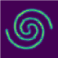
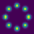
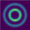
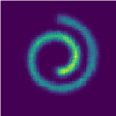
Figure 2: Visualization of learned energy model and sampler. From left to right: 2spirals, 8gaussians, checkerboard, circles, moons, pinwheel, swissroll. Due to the limited space, please refer to Figure A.1 in appendix for the visualization of training samples.

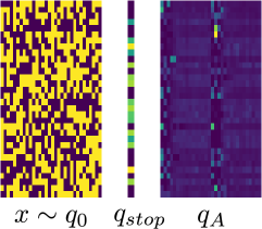
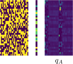
Sampler visualization in 2D space	Run edit on initial $x_{0}$	Run edit on $x$ from sampler

Figure 3: Visualization of learned local search sampler in 2D (left) and original discrete Gray code (mid + right) space. See Section 5.1 for more information.

Table 1: Synthetic results with MMD-hamming ($\mathbf{\times 1e^{-3}}$) as evaluation metric, and the lower the better. * denote the discrete adaptation of its original method for continuous domain.

		2spirals	8gaussians	circles	moons	pinwheel	swissroll	checkerboard
	PCD-10* [10, 12]	34.73	0.3	-0.3	0.48	-0.42	-0.49	-1.04
	ADE* [8]	33.4	-0.28	2.01	2.16	7.64	6.12	-0.69
	ALOE	30.37	-0.97	-0.83	-0.64	-0.64	-0.58	-1.7
Ablation	ADE-fac	236.6	65.7	261.7	248.6	187.2	95.3	78.2
	ALOE-fac-noEdit	51.24	91.2	5.97	76.8	59.7	15	2.98
	ALOE-fac-edit	32.6	3	-1.5	1.27	5.02	0.44	-2.03
Other	AutoRegressive	32.7	-0.3	-0.8	-0.45	-1.27	0.31	-0.2
	VAE	35.2	2.09	0.16	1.1	0.85	2.05	-0.77

Main results: To quantitatively evaluate different methods, we use MMD [62] with linear kernel (which corresponds to $32-\text{HammingDistance}$) to evaluate the empirical distribution between true samples and samples from the learned energy function. To obtain samples from $f$, we run $20\times 32$ steps of Gibbs sampling and collect 4000 samples. We can see from Table 1 that ALOE consistently outperforms alternatives across all datasets. ADE variant is worse than PCD on some datasets, as REINFORCE based approaches typically requires careful treatment of the gradient variance.

We also use VAE [63] or autoregressive model to learn the discrete distribution, where the results are shown in the “Other” section of Table 1. Note that these models are different, so the numerical comparison is mainly for the sake of completeness. ALOE mainly focuses on learning a given energy based model, rather than proposing a new probabilistic model.

Visualization: We first visualize the learned score function and sampler in Figure 2. To plot the heat map, we first uniformly sample 10k 2D points with each dimension in $[-4,4]$. Then we convert the floating-point numbers to Gray code to evaluate and visualize the score under learned $f$. Please refer to Appendix A.1 for more visualizations about baselines. In Figure 3, we visualize the learned local search sampler in both discrete space and 2D space by decoding the Gray code. We can see ALOE gets reasonable quality even with a weak $q_{0}(x)=\prod_{i=1}^{32}q_{0}(x[i])$, and it automatically adapts the refinement steps according to the quality of $q_{0}$.

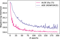
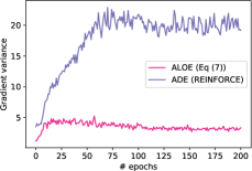
Negative Log-likelihood	Gradient Variance

Figure 4: Training objective and gradient variance.

Gradient variance: Here we empirically justify the necessity of the variational power iteration objective design in (7) against the REINFORCE objective. We train ADE and ALOE (with only $q_{0}$ for comparison) on pinwheel data, and plot the negative log-likelihood of EBM (estimated via importance sampling) and the Monte Carlo estimation of gradient variance in Figure 4. We can clearly see ALOE enjoys lower variance and thus faster and better convergence than REINFORCE based methods for EBMs.

Ablation: Here we try to justify the necessity of both local edits and the variational power iteration objective. a)To justify the local edits, we use a fully factorized initial $q_{0}$, and compare ALOE-fac-noEdit (no further edits) against ALOE-fac-edit (with $\leq$16 edits). ALOE-fac-edit performs much better than the noEdit version. We use a weak $q_{0}$ here since we don’t need many edits when $q_{0}$ is the powerful MLP with no parameter sharing (which is not feasible in realistic tasks). Nevertheless, ALOE automatically learns to adapt number of edits as studied in Figure 3 left. b)We also show the objective in (7) achieves better results than the REINFORCE objective from ADE.

5.2 Generative fuzzing

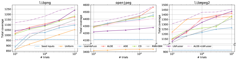
Figure 5: Coverage statistics on different softwares with different amount of test inputs generated.

A critical step in software quality assurance is to generate random inputs to test the software for vulnerabilities, also known as fuzzing [64]. Recently learning based approaches have shown promising results for fuzzing [4, 65]. In this section we focus on the generative fuzzing task, where we first learn a generative model from existing seed inputs (a set of software-dependent binary files) and then generate new inputs from the model to test the software.

Experiment setup: We collect three software binaries (namely libpng, libmpeg2 and openjpeg) from OSS-Fuzz as test target. For all ML based methods, we use the seed inputs that come with OSS-Fuzz to learn the generative model. As each test input for software can be very large (e.g., a media file for libmpeg2), we train a truncated EBM with a window size of 64. Specifically, we learn a conditional EBM $f(x|y)$, where $x\in\{0,\ldots,255\}^{64}$ is a chunk of byte data and $y\in\{0,1,\ldots\}$ is the position of this chunk in its original file.

During inference, instead of generating test inputs from scratch (which would be too difficult to generate 1M bytes while still being parsable by the target software), we use the learned model to modify the seed inputs instead. To modify $i$-th byte of the byte string $\mathbf{x}$ using learned EBM, we sample the byte $b\propto\exp(f([\mathbf{x}_{i-31},\ldots,b,\ldots,\mathbf{x}_{i+32}]|i))$ by conditioning on its surrounding context.

We compare against the following generative model based methods:

• Learn&Fuzz [4]: this method learns an autoregressive model from sequences of byte data. We adapt its open-source implementation. To use the autoregressive model for mutating the seed inputs, we perform the edit by sampling $x_{i}\sim p(\cdot|\mathbf{x}_{0:i-1})$ conditioned on its prefix.

• ADE [8]: This method parameterizes the model and initial sampler $q_{0}$ in the same way as ALOE.

• CD: As PCD is not directly applicable for conditional EBM learning, we use CD instead.

• RNN-EBM: It treats the autoregressive model learned by Learn&Fuzz as an EBM, and mutates the seed inputs in the same way as other EBM based mutations.

We also use uniform sampling (denoted as Uniform) over byte modifications as a baseline, and include LibFuzzer coverage with the same seed inputs as reference. Note that LibFuzzer is a well engineered system used commercially for fuzzing, which gathers feedback from the test program by monitoring which branches are taken during execution. Therefore, this is supposed to be superior to generative approaches like EBMs, which do not incorporate this feedback.

For all methods, we generate up to 100k inputs with 100 modifications for each. The main evaluation measure is coverage, which measures how many of the lines of code, branches, and so on, are exercised by the test inputs; higher is better. This statistic is reported by LibFuzzer.

Results are shown in Figure 5. Overall the discrete EBM learned by ALOE consistently outperforms the autoregressive model. Suprisingly, the coverage obtained by ALOE is comparable or even better than LibFuzzer on some targets, despite the fact that LibFuzzer has access to more information about the program execution. In the long run, we believe that this additional information will allow LibFuzzer to perform the best, it is still appealing that ALOE has high sample efficiency initially. Regarding several EBM based methods, we can see CD is comparable on libpng but for large target like openjpeg it performs much worse. ADE performs good initially on some targets but gets worse in the long run. Our hypothesis is that it is due to the lack of diversity, which suggests a potential mode drop problem that is common in REINFORCE based approaches. The uniform baseline performs worst in most cases, except on libmpeg2 early stage. Our hypothesis is that the uniform fuzzer quickly triggers many branches that raise formatting errors, which explains its high coverage initially.

We also combine the test inputs generated by LibFuzzer and ALOE (the orange dotted curve, for which the $x$-axis shows the number of samples from each method). The coverage of this combined set of inputs is better than either individually, showing that the methods are complementary.

5.3 Program Synthesis

In program synthesis, the task is to predict the source code of a program given a few input-output (IO) pairs that specify its behavior. We evaluate ALOE on the RobustFill task [3] of generating string transformations.The purpose here is to evaluate the effect of proposed local edits in our sampler, so the other methods like ADE or PCD are not applicable here. For full details, see Appendix A.2.

Table 2: Program synthesis accuracy on RobustFill tasks [3].

	Top-1 Beam-1	Top-1 Beam-10	Top-10 Beam-10
seq2seq-init	45.86	55.49	58.66
seq2seq-tune	47.86	57.52	60.62
ALOE	53.57	61.99	65.29

Experiment setup: Data is generated synthetically, following Devlin et al. [3]. Each example in the data set is a synthesis task where the input is four IO pairs, the target is a program, and a further six IO pairs are held out for evaluation. The training data is generated on the fly, while we keep 10k test examples for evaluation. Each target program consists of at most 10 sub-expressions in a domain-specific languages which includes string concatenation, substring operations, etc. We report accuracy, which measures when the predicted program is consistent with all $10$ IO pairs.

For ALOE we learn a conditional sampler $q(x|z)$ where $x$ is the program syntax tree, and $z$ is the list of input-output pairs. We compare with 3-layer seq2seq model for program prediction. Both seq2seq and ALOE share the same IO-pair encoder. As mentioned in Section 3.2, the initial distribution $q_{0}$ is the same as seq2seq autoregressive model, while subsequent modifications $A(x_{i+1}|x_{i})$ adds/deletes/replaces one of the subexpressions. We train baseline seq2seq with 483M examples (denoted as seq2seq-init), and fine-tune with additional 264M samples (denoted as seq2seq-tune) with reduced learning rate. ALOE initializes $q_{0}$ from seq2seq-init and set it to be fixed, and train the editor $q_{A}(\cdot|\cdot)$ with same additional number of samples with the shortest edit importance proposal (14).

Results: We report the top-$k$ accuracy with different beam-search sizes in Table 2. We can see ALOE outperforms the seq2seq baseline by a large margin. Although the initial sampler $q_{0}$ is the same as seq2seq-init, the editor $q_{A}(\cdot|\cdot)$ is able to further locate and correct sub-expressions of the initial prediction. In the figure to the right of Table 2, We also visualize the number of edits our sampler makes on the test set. In most cases $q_{0}$ already produces correct results, and the sampler correctly learns to stop at step $0$. From 1 to 9 edits we can see the editor indeed improved from $q_{0}$ by a large margin. There are many cases which require $10$ or more edits, in which case we truncate the local search steps to 10. Some of them are difficult cases where the sampler learns to ask for more steps, while for others the sampler keeps modifying to semantically equivalent programs.

6 Conclusion

In this paper, we propose ALOE, a new algorithm for learning discrete EBMs for both conditional and unconditional cases. ALOE learns a sampler that is parameterized as a local search algorithm for proposing negative samples in contrastive learning framework. With an efficient importance reweighted gradient estimator, we are able to train both the sampler and the EBM with a variational power iteration principle. Experiments on both synthetic datasets and real-world software testing and program synthesis tasks show that both the learned EBM and local search sampler outperforms the autoregressive alternative. Future work includes better approximation of learning local search algorithms, as well as extending it to other discrete domains like chemical engineering and NLP.

Broader Impact

We hope our new algorithm ALOE for learning discrete EBMs can be useful for different domains with discrete structures, and it furthers the general research efforts in this direction of generative models of discrete structures. In this paper, we present its application to program synthesis and software fuzzing. A positive outcome of improved performance in program synthesis would be that it can help democratize the task of programming by allowing people to express their desired intent using input-output examples without the need of learning complex programming languages. Similarly, a positive outcome of improvements in software fuzzing could allow software developers to identify bugs and vulnerabilities quicker and in turn improve software reliability and robustness.

A possible negative outcome could be that malicious attackers might also use such technology to discover software vulnerabilities and use it for undesirable purposes [66]. However, this outcome is not specific to our technique but more generally applicable to the large research field of software fuzzing, and there is a large amount of work in the fuzzing field for accounting ethical considerations. For example, the vulnerabilities typically found by fuzzers is first responsibly disclosed to corresponding software teams [67] that gives them enough time to patch the vulnerabilities before the bugs and vulnerabilities are released publicly.

Appendix

Appendix A More experiment details

A.1 Synthetic experiments

Baseline configuration

We adapt two most recent techniques for learning EBMs into discrete case, namely Du and Mordatch [12] and Dai et al. [8]. Specifically:

• PCD based:  Du and Mordatch [12] extends the PCD method with replay buffer and random restart. We adapt these tricks in learning discrete EBMs. Specifically, we use Gibbs sampling for $K\times 32$-steps as the MCMC sampler, where $K$ is set to 10. Instead of always inheriting from previous MCMC samples, we tune the restart rate in $\{0.05,0.1,1\}$.

• ADE based: ADE solves the same minimax problem in Eq (4), but instead directly minimizes the objective $L(q):=-\mathbb{E}_{x\sim q}\left[f(x)\right]-H(q)$. To make ADE work in discrete case, optimizing $L(q)$ requires the policy gradient technique with variance reduction [34, 68, 22, 69], where the gradient estimator becomes $\nabla_{q}L(q)=\mathbb{E}_{x\sim q}\nabla\log q(x)(-f(x)-\log q(x)-1)$. This also resembles the learning of GAN [70] on sequences [71] or graphs [72], except the additional entropy regularization term and constant. We use A2C [34] to learn ADE for discrete EBMs. As ADE uses alternating minimization for minimax problem, we tune the learning rate ratio and synchronization frequency between energy function and sampler learning in $\{0.2,0.5,1\}$ and $\{1:1,1:3,1:5\}$, respectively.

More visualizations

2spirals	8gaussians	checkerboard	circles	moons	pinwheel	swissroll

Figure A.1: 2D visualization of samples from the ground truth distribution.

PCD*
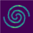
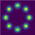
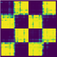
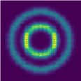
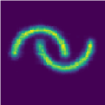
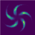
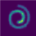
ADE*
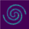
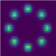
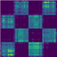
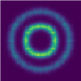
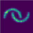
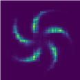
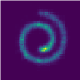
ALOE
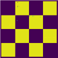
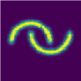
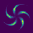
2spirals	8gaussians	checkerboard	circles	moons	pinwheel	swissroll

Figure A.2: visualization of learned discrete EBMs using different methods.

In Figure A.1 we also visualize the samples obtained from the ground truth distribution and visualize them in 2D space. Compared to Figure 2 we can see our learned sampler can almost perfectly recover the true distribution. The checkerboard seems to be the most difficult one among these datasets, as for both PCD and ADE baselines the learned model is much worse than the one learned by ALOE. We find that in this case the distribution is not smooth as it has sharp boundaries for each “square” in the distribution. Thus below we study how the learned sampler behaves for ADE algorithm in this case.

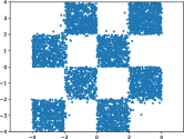
$q_{0}=$MLP	$q_{0}=$RNN

Figure A.3: ADE with different samplers.

In Figure 3 in main paper we have studied ALOE with different design choices of $q_{0}$, where a weak $q_{0}$ like fully factored distribution can still get reasonable results. Instead in Figure A.3 we can see that, for ADE, different parameterizations of the sampler will make quite different behaviors. The MLP sampler is an autoregressive one with non-sharing parameters, while the RNN sampler has the shared parameters across different steps. This clearly shows the limitation of autoregressive model with parameter sharing, and also the necessity of learning sampler with local search to improve the weak initial sampler $q_{0}$.

Implementation details

Here we provide more details on the instantiation of ALOE on the synthetic tasks. Below we first cover the parameterization details.

The energy function is an MLP with dimensions of $[32,256,256,256,1]$, where 32 is the input size, and $256$ is the hidden layer size. We use ELU as the activation function.

For ADE and ALOE, the $q0$ is parameterized with either autoregressive model or a factorized model. For the factorized model, we simply learn 32-dimensional vector that represents the logits of each dimension independently. For the autoregressive model, there can be two choices. The first one uses LSTM (which we denote as RnnSampler) to encode the bits, where LSTM has hidden size of 256 and 1 layer. All the dimensions share the same predictor that predicts the binary bit from the latent embedding obtained by LSTM. The predictor is an MLP with size $[256,512,2]$ with ELU activation. Another alternative is to use MLP to encode the bits, as we know the maximum length is 32 beforehand (which is not practical in general). This way we encode the history using 31 MLPs, where the $i$-th MLP has size $[i,512,512,256]$ that embeds the prefix of length $i$, and use the shared predictor to predict the bit at current position.

ALOE has additional components, which are editor $q_{A}(\cdot|\cdot)$ and stop policy $q_{\text{stop}}$. The editor only needs to predict the location for modification, as once the location is given one can simply flip that bit. It is parameterized into $[32,512,512,32]$ with ELU as activation function and softmax at the end. The stop policy is parameterized by an MLP with layers $[32,512,512,1]$ with ELU activation and sigmoid in the last output.

We use the Inverse proposal where $A^{\prime}(\cdot|\cdot)$ is a uniform distribution that samples a random location for modification. To avoid sampling the same position twice, we first permute the locations and then pick the first $k$ locations as the proposal trajectory, where $k$ is the number of edits that is sampled from a geometric distribution, with the truncation at 16.

A.2 Program synthesis experiments

Grammar: We use the following grammar for RobustFill programs.

24ex 0.5ex ¡program¿ $\rightarrow$ ¡ExprList¿

¡ExprList¿ $\rightarrow$ ¡expr¿ — ¡expr¿ ¡ExprList¿

¡expr¿ $\rightarrow$ ‘ConstStr’ ¡ConstExpr¿ — ‘SubStr’ ¡SubstrExpr¿

¡ConstExpr¿ $\rightarrow$ ‘]’ — ‘,’ — ‘-’ — ‘.’ — ‘@’ — ‘” — ‘”’ — ‘(’ — ‘)’ — ‘:’ — ‘%’

¡SubstrExpr¿ $\rightarrow$ ¡Pos¿ ¡Pos¿

¡Pos¿ $\rightarrow$ ¡ConstPos¿ — ¡RegPos¿

¡ConstPos¿ $\rightarrow$ -4 — -3 — -2 — -1 — 0 — 1 — 2 — 3 — 4

¡RegPos¿ $\rightarrow$ ¡ConstTok¿ — ¡RegexTok¿

¡ConstTok¿ $\rightarrow$ ¡ConstExpr¿ ¡p2¿ ¡direct¿

¡RegexTok¿ $\rightarrow$ ¡RegexStr¿ ¡p2¿ ¡direct¿

¡p2¿ $\rightarrow$ ¡ConstPos¿

¡direct¿ $\rightarrow$ ‘Start’ — ‘End’

¡RegexStr¿ $\rightarrow$ ‘[A-Z]([a-z])+’ — ‘[A-Z]+’ — ‘[a-z]+’ — ‘
d+’ — ‘[a-zA-Z]+’ — ‘[a-zA-Z0-9]+’ — ‘
s+’ — ‘^’ — ‘$’

Data generator: We use following configurations for generating synthetic data for program synthesis:

• The maximum number of types of tokens in input strings is set to 5.

• The maximum length of input strings is 20.

• The maximum length of output strings is 50.

• The total number of input-output examples per synthesis task is 10.

• The number of public input-output example pairs is 4.

• The number of private input-output example pairs is 6.

The learned synthesizer uses the 4 public IO pairs for synthesize the program, and evaluate against all 10 IO pairs. It is considered correct if it is consistent with these 10 IO pairs.

Parameterization: We use a 3-layer LSTM with hidden size of 256 to encode each input and output sequences, respectively. Then each IO pair is represented by concatenating the sequence embeddings of input and output strings. The set of inputs is obtained by max-pooling over the IO-pair embeddings, which will be served as the context for program synthesis.

For $q_{0}$ we use a 3-layer LSTM with hidden size of 256 for predicting program tokens. For ALOE we parameterize the $q_{A}$ with two components: the position predictor $q_{\text{\tiny pos}}$ and the modified expression $q_{\text{\tiny expr}}$. $q_{\text{\tiny pos}}$ embeds the current program using 3-layer bidirectional LSTM, and predict the position using pointer mechanism [36]. Note that the selected position must be the start or end of an existing $<expr>$ in above grammar, which indicates whether we want to modify or insert a new $<expr>$ in this position. $q_{\text{\tiny expr}}$ predicts the new expression using another 3-layer LSTM, and is allowed to make empty prediction (which corresponds to delete an expression in current program). As the program heavily relies on the context free grammar to make it valid, we utilize the technique in grammarVAE [73] to mask out invalid production rules during program generation.

A.3 Fuzzing experiment

Software	# seed files	file size (bytes)	# training samples for ALOE
libpng	170	104 - 12,901	146,507
openjpeg	36	233 - 7,885,684	27,572,688
libmpeg2	131	10,581 - 50,000	6,119,237

Table A.1: Data statistics for generative fuzzing experiments. We use window size 64 for ALOE to obtain chunks of data from the raw byte streams.

Data statistics: We test different approaches against three target softwares. The OSS-Fuzz project comes with different set of seed inputs for different target softwares. These inputs are served as training samples for both ALOE and Godefroid et al. [4], and will be used as seed inputs for libFuzzer as well. Table A.1 displays the data statistics. Note that ALOE trains a conditional EBM with chunked data from the original raw byte streams, in order to handle huge files. We use chunk size 64 by default. Thus for a file with size $L$ where $L\geq 64$, there will be $L-64+1$ training samples for ALOE.

Parameterization: We use a three-layer MLP to parameterize the energy function, where for the input layer, we use embedding size equals to 4 for the byte string. For the negative sampler, we parameterize $q_{0}$ with LSTM. $q_{A}$ consists of two parts, namely $q_{\text{\tiny pos}}$ which predicts which position to modify using an MLP, and $q_{\text{\tiny value}}$ which predicts a new value for that position using another MLP. We use Eq (13) for training such EBM.

References

- Tai et al. [2015] Kai Sheng Tai, Richard Socher, and Christopher D Manning. Improved semantic representations from tree-structured long short-term memory networks. arXiv preprint arXiv:1503.00075, 2015.
- Zhang et al. [2016] Xingxing Zhang, Liang Lu, and Mirella Lapata. Top-down tree long Short-Term memory networks. In North American Chapter of the Association for Computational Linguistics (NAACL), 2016.
- Devlin et al. [2017] Jacob Devlin, Jonathan Uesato, Surya Bhupatiraju, Rishabh Singh, Abdel-rahman Mohamed, and Pushmeet Kohli. Robustfill: Neural program learning under noisy i/o. In Proceedings of the 34th International Conference on Machine Learning-Volume 70, pages 990–998. JMLR. org, 2017.
- [4] Patrice Godefroid, Hila Peleg, and Rishabh Singh. Learn&fuzz: Machine learning for input fuzzing. In 2017 32nd IEEE/ACM International Conference on Automated Software Engineering (ASE), pages 50–59. IEEE.
- LeCun et al. [2006] Yann LeCun, Sumit Chopra, Raia Hadsell, M Ranzato, and F Huang. A tutorial on energy-based learning. 2006.
- Scarselli et al. [2008] Franco Scarselli, Marco Gori, Ah Chung Tsoi, Markus Hagenbuchner, and Gabriele Monfardini. The graph neural network model. IEEE Transactions on Neural Networks, 20(1):61–80, 2008.
- Kipf and Welling [2016] Thomas N Kipf and Max Welling. Semi-supervised classification with graph convolutional networks. arXiv preprint arXiv:1609.02907, 2016.
- Dai et al. [2019a] Bo Dai, Zhen Liu, Hanjun Dai, Niao He, Arthur Gretton, Le Song, and Dale Schuurmans. Exponential family estimation via adversarial dynamics embedding. In Advances in Neural Information Processing Systems, pages 10977–10988, 2019a.
- Hinton [2002] Geoffrey E Hinton. Training products of experts by minimizing contrastive divergence. Neural computation, 14(8):1771–1800, 2002.
- Tieleman [2008] Tijmen Tieleman. Training restricted boltzmann machines using approximations to the likelihood gradient. In Proceedings of the 25th international conference on Machine learning, pages 1064–1071, 2008.
- Wu et al. [2018] Ying Nian Wu, Jianwen Xie, Yang Lu, and Song-Chun Zhu. Sparse and deep generalizations of the frame model. Annals of Mathematical Sciences and Applications, 3(1):211–254, 2018.
- Du and Mordatch [2019] Yilun Du and Igor Mordatch. Implicit generation and generalization in energy-based models. arXiv preprint arXiv:1903.08689, 2019.
- Besag [1975] Julian Besag. Statistical analysis of non-lattice data. Journal of the Royal Statistical Society: Series D (The Statistician), 24(3):179–195, 1975.
- Hyvärinen [2005] Aapo Hyvärinen. Estimation of non-normalized statistical models by score matching. Journal of Machine Learning Research, 6(Apr):695–709, 2005.
- Dai et al. [2018] Bo Dai, Hanjun Dai, Arthur Gretton, Le Song, Dale Schuurmans, and Niao He. Kernel exponential family estimation via doubly dual embedding. arXiv preprint arXiv:1811.02228, 2018.
- Arbel et al. [2020] Michael Arbel, Liang Zhou, and Arthur Gretton. Kale: When energy-based learning meets adversarial training. arXiv preprint arXiv:2003.05033, 2020.
- Williams [1992] Ronald J Williams. Simple statistical gradient-following algorithms for connectionist reinforcement learning. Machine learning, 8(3-4):229–256, 1992.
- Glynn [1990] Peter W Glynn. Likelihood ratio gradient estimation for stochastic systems. Communications of the ACM, 33(10):75–84, 1990.
- Bengio et al. [2013] Yoshua Bengio, Nicholas Léonard, and Aaron Courville. Estimating or propagating gradients through stochastic neurons for conditional computation. arXiv preprint arXiv:1308.3432, 2013.
- Jang et al. [2016] Eric Jang, Shixiang Gu, and Ben Poole. Categorical reparameterization with gumbel-softmax. arXiv preprint arXiv:1611.01144, 2016.
- Maddison et al. [2016] Chris J Maddison, Andriy Mnih, and Yee Whye Teh. The concrete distribution: A continuous relaxation of discrete random variables. arXiv preprint arXiv:1611.00712, 2016.
- Tucker et al. [2017] George Tucker, Andriy Mnih, Chris J Maddison, John Lawson, and Jascha Sohl-Dickstein. Rebar: Low-variance, unbiased gradient estimates for discrete latent variable models. In Advances in Neural Information Processing Systems, pages 2627–2636, 2017.
- Tucker et al. [2018] George Tucker, Surya Bhupatiraju, Shixiang Gu, Richard E Turner, Zoubin Ghahramani, and Sergey Levine. The mirage of action-dependent baselines in reinforcement learning. arXiv preprint arXiv:1802.10031, 2018.
- Yin et al. [2019] Mingzhang Yin, Yuguang Yue, and Mingyuan Zhou. Arsm: Augment-reinforce-swap-merge estimator for gradient backpropagation through categorical variables. arXiv preprint arXiv:1905.01413, 2019.
- Wainwright and Jordan [2008] M J Wainwright and M I Jordan. Graphical models, exponential families, and variational inference. Foundations and Trends in Machine Learning, 1(1-2):1–305, 2008.
- Hochreiter and Schmidhuber [1997] Sepp Hochreiter and Jürgen Schmidhuber. Long short-term memory. Neural computation, 9(8):1735–1780, 1997.
- [27] Radford M Neal et al. Mcmc using hamiltonian dynamics.
- Welling and Teh [2011] Max Welling and Yee W Teh. Bayesian learning via stochastic gradient langevin dynamics. In Proceedings of the 28th international conference on machine learning (ICML-11), pages 681–688, 2011.
- Xie et al. [2018] Jianwen Xie, Yang Lu, Ruiqi Gao, and Ying Nian Wu. Cooperative learning of energy-based model and latent variable model via mcmc teaching. In Thirty-Second AAAI Conference on Artificial Intelligence, 2018.
- Hinton et al. [1995] Geoffrey E Hinton, Peter Dayan, Brendan J Frey, and Radford M Neal. The” wake-sleep” algorithm for unsupervised neural networks. Science, 268(5214):1158–1161, 1995.
- Dayan et al. [1995] Peter Dayan, Geoffrey E Hinton, Radford M Neal, and Richard S Zemel. The helmholtz machine. Neural computation, 7(5):889–904, 1995.
- Li et al. [2018] Yujia Li, Oriol Vinyals, Chris Dyer, Razvan Pascanu, and Peter Battaglia. Learning deep generative models of graphs. arXiv preprint arXiv:1803.03324, 2018.
- [33] Jacob Steinhardt and Percy Liang. Learning fast-mixing models for structured prediction.
- Mnih and Gregor [2014] Andriy Mnih and Karol Gregor. Neural variational inference and learning in belief networks. arXiv preprint arXiv:1402.0030, 2014.
- Chen and Tian [2019] Xinyun Chen and Yuandong Tian. Learning to perform local rewriting for combinatorial optimization. In Advances in Neural Information Processing Systems, pages 6278–6289, 2019.
- Vinyals et al. [2015] Oriol Vinyals, Meire Fortunato, and Navdeep Jaitly. Pointer networks. In Advances in neural information processing systems, pages 2692–2700, 2015.
- Yu et al. [2020] Lantao Yu, Yang Song, Jiaming Song, and Stefano Ermon. Training deep energy-based models with f-divergence minimization. arXiv preprint arXiv:2003.03463, 2020.
- Kim and Bengio [2016] Taesup Kim and Yoshua Bengio. Deep directed generative models with energy-based probability estimation. arXiv preprint arXiv:1606.03439, 2016.
- Nijkamp et al. [2019] Erik Nijkamp, Mitch Hill, Song-Chun Zhu, and Ying Nian Wu. Learning non-convergent non-persistent short-run mcmc toward energy-based model. In Advances in Neural Information Processing Systems, pages 5233–5243, 2019.
- Kuleshov and Ermon [2017] Volodymyr Kuleshov and Stefano Ermon. Neural variational inference and learning in undirected graphical models. In Advances in Neural Information Processing Systems, pages 6734–6743, 2017.
- Li et al. [2020] Chongxuan Li, Chao Du, Kun Xu, Max Welling, Jun Zhu, and Bo Zhang. To relieve your headache of training an mrf, take advil. In International Conference on Learning Representations, 2020. URL https://openreview.net/forum?id=Sylgsn4Fvr.
- Bakhtin et al. [2020] Anton Bakhtin, Yuntian Deng, Sam Gross, Myle Ott, Marc’Aurelio Ranzato, and Arthur Szlam. Energy-based models for text, 2020.
- Deng et al. [2020] Yuntian Deng, Anton Bakhtin, Myle Ott, Arthur Szlam, and Marc’Aurelio Ranzato. Residual energy-based models for text generation. arXiv preprint arXiv:2004.11714, 2020.
- Gutmann and Hyvärinen [2010] Michael Gutmann and Aapo Hyvärinen. Noise-contrastive estimation: A new estimation principle for unnormalized statistical models. In Proceedings of the Thirteenth International Conference on Artificial Intelligence and Statistics, pages 297–304, 2010.
- Belanger and McCallum [2016] David Belanger and Andrew McCallum. Structured prediction energy networks. In International Conference on Machine Learning, pages 983–992, 2016.
- Belanger et al. [2017] David Belanger, Bishan Yang, and Andrew McCallum. End-to-end learning for structured prediction energy networks. In Proceedings of the 34th International Conference on Machine Learning-Volume 70, pages 429–439. JMLR. org, 2017.
- Taskar et al. [2004] Ben Taskar, Carlos Guestrin, and Daphne Koller. Max-margin markov networks. In Advances in neural information processing systems, pages 25–32, 2004.
- He et al. [2014] He He, Hal Daume III, and Jason M Eisner. Learning to search in branch and bound algorithms. In Advances in neural information processing systems, pages 3293–3301, 2014.
- Chang et al. [2015] Kai-Wei Chang, Akshay Krishnamurthy, Alekh Agarwal, John Langford, and Hal Daumé III. Learning to search better than your teacher. 2015.
- Song et al. [2018] Jialin Song, Ravi Lanka, Albert Zhao, Aadyot Bhatnagar, Yisong Yue, and Masahiro Ono. Learning to search via retrospective imitation. arXiv preprint arXiv:1804.00846, 2018.
- Guez et al. [2018] Arthur Guez, Théophane Weber, Ioannis Antonoglou, Karen Simonyan, Oriol Vinyals, Daan Wierstra, Rémi Munos, and David Silver. Learning to search with mctsnets. arXiv preprint arXiv:1802.04697, 2018.
- Xia et al. [2017] Yingce Xia, Fei Tian, Lijun Wu, Jianxin Lin, Tao Qin, Nenghai Yu, and Tie-Yan Liu. Deliberation networks: Sequence generation beyond one-pass decoding. In Advances in Neural Information Processing Systems, pages 1784–1794, 2017.
- Tran et al. [2019] Dustin Tran, Keyon Vafa, Kumar Agrawal, Laurent Dinh, and Ben Poole. Discrete flows: Invertible generative models of discrete data. In Advances in Neural Information Processing Systems, pages 14692–14701, 2019.
- Hoogeboom et al. [2019] Emiel Hoogeboom, Jorn Peters, Rianne van den Berg, and Max Welling. Integer discrete flows and lossless compression. In Advances in Neural Information Processing Systems, pages 12134–12144, 2019.
- Shi et al. [2020] Chence Shi, Minkai Xu, Zhaocheng Zhu, Weinan Zhang, Ming Zhang, and Jian Tang. Graphaf: a flow-based autoregressive model for molecular graph generation. arXiv preprint arXiv:2001.09382, 2020.
- Madhawa et al. [2019] Kaushalya Madhawa, Katushiko Ishiguro, Kosuke Nakago, and Motoki Abe. Graphnvp: An invertible flow model for generating molecular graphs. arXiv preprint arXiv:1905.11600, 2019.
- Stern et al. [2019] Mitchell Stern, William Chan, Jamie Kiros, and Jakob Uszkoreit. Insertion transformer: Flexible sequence generation via insertion operations. arXiv preprint arXiv:1902.03249, 2019.
- Gu et al. [2019] Jiatao Gu, Changhan Wang, and Junbo Zhao. Levenshtein transformer. In Advances in Neural Information Processing Systems, pages 11179–11189, 2019.
- Ghazvininejad et al. [2019] Marjan Ghazvininejad, Omer Levy, Yinhan Liu, and Luke Zettlemoyer. Constant-time machine translation with conditional masked language models. arXiv preprint arXiv:1904.09324, 2019.
- Grathwohl et al. [2018] Will Grathwohl, Ricky TQ Chen, Jesse Bettencourt, Ilya Sutskever, and David Duvenaud. Ffjord: Free-form continuous dynamics for scalable reversible generative models. arXiv preprint arXiv:1810.01367, 2018.
- Clevert et al. [2015] Djork-Arné Clevert, Thomas Unterthiner, and Sepp Hochreiter. Fast and accurate deep network learning by exponential linear units (elus). arXiv preprint arXiv:1511.07289, 2015.
- Gretton et al. [2012] Arthur Gretton, Karsten M Borgwardt, Malte J Rasch, Bernhard Schölkopf, and Alexander Smola. A kernel two-sample test. Journal of Machine Learning Research, 13(Mar):723–773, 2012.
- Kingma and Welling [2013] Diederik P Kingma and Max Welling. Auto-encoding variational bayes. arXiv preprint arXiv:1312.6114, 2013.
- Miller et al. [1990] Barton P Miller, Louis Fredriksen, and Bryan So. An empirical study of the reliability of unix utilities. Communications of the ACM, 33(12):32–44, 1990.
- Dai et al. [2019b] Hanjun Dai, Yujia Li, Chenglong Wang, Rishabh Singh, Po-Sen Huang, and Pushmeet Kohli. Learning transferable graph exploration. In Advances in Neural Information Processing Systems, pages 2514–2525, 2019b.
- Brundage et al. [2018] Miles Brundage, Shahar Avin, Jack Clark, Helen Toner, Peter Eckersley, Ben Garfinkel, Allan Dafoe, Paul Scharre, Thomas Zeitzoff, Bobby Filar, et al. The malicious use of artificial intelligence: Forecasting, prevention, and mitigation. arXiv preprint arXiv:1802.07228, 2018.
- Householder et al. [2017] Allen D Householder, Garret Wassermann, Art Manion, and Chris King. The cert guide to coordinated vulnerability disclosure. Technical report, Carnegie-Mellon Univ Pittsburgh Pa Pittsburgh United States, 2017.
- Gu et al. [2015] Shixiang Gu, Sergey Levine, Ilya Sutskever, and Andriy Mnih. Muprop: Unbiased backpropagation for stochastic neural networks. arXiv preprint arXiv:1511.05176, 2015.
- Grathwohl et al. [2017] Will Grathwohl, Dami Choi, Yuhuai Wu, Geoffrey Roeder, and David Duvenaud. Backpropagation through the void: Optimizing control variates for black-box gradient estimation. arXiv preprint arXiv:1711.00123, 2017.
- Goodfellow et al. [2014] Ian Goodfellow, Jean Pouget-Abadie, Mehdi Mirza, Bing Xu, David Warde-Farley, Sherjil Ozair, Aaron Courville, and Yoshua Bengio. Generative adversarial nets. In Advances in neural information processing systems, pages 2672–2680, 2014.
- Yu et al. [2017] Lantao Yu, Weinan Zhang, Jun Wang, and Yong Yu. Seqgan: Sequence generative adversarial nets with policy gradient. In Thirty-First AAAI Conference on Artificial Intelligence, 2017.
- De Cao and Kipf [2018] Nicola De Cao and Thomas Kipf. Molgan: An implicit generative model for small molecular graphs. arXiv preprint arXiv:1805.11973, 2018.
- Kusner et al. [2017] Matt J Kusner, Brooks Paige, and José Miguel Hernández-Lobato. Grammar variational autoencoder. In Proceedings of the 34th International Conference on Machine Learning-Volume 70, pages 1945–1954. JMLR. org, 2017.