Criticality in Cell Adhesion

Abstract

We illuminate the many-body effects underlying the structure, formation, and dissolution of cellular adhesion domains in the presence and absence of forces. We consider mixed Glauber-Kawasaki dynamics of a two-dimensional model of nearest-neighbor interacting adhesion bonds with intrinsic binding-affinity under the action of a shared pulling or pushing force. We consider adhesion bonds that are immobile due to being anchored to the underlying cytoskeleton as well as adhesion molecules that are transiently diffusing. Highly accurate analytical results are obtained on the pair-correlation level of the Bethe-Guggenheim approximation for the complete thermodynamics and kinetics of adhesion clusters of any size, including the thermodynamic limit. A new kind of dynamical phase transition is uncovered — the mean formation and dissolution times per adhesion bond change discontinuously with respect to the bond-coupling parameter. At the respective critical points cluster formation and dissolution are fastest, while the statistically dominant transition path undergoes a qualitative change — the entropic barrier to complete binding/unbinding is rate-limiting below, and the phase transition between dense and dilute phases above the dynamical critical point. In the context of the Ising model the dynamical phase transition reflects a first-order discontinuity in the magnetization-reversal time. Our results provide a potential explanation for the mechanical regulation of cell adhesion, and suggest that the quasi-static and kinetic response to changes in the membrane stiffness or applied forces is largest near the statical and dynamical critical point, respectively.

I Introduction

Cell adhesion refers to the specific binding of cells to neighboring cells or the extracellular matrix. It plays a major role in cell regulation [1], intercellular communication [2], immune response [3], wound healing [4], morphogenesis [5], cellular function [6], and tumorigenesis [7, 8]. Cellular adhesion domains form as a result of the association of transmembrane cellular adhesion molecules (CAMs) that interact with the actin cytoskeleton [9] and can translocate over the membrane [10]. There are four major superfamilies of CAMs; the immunoglobulins, integrins, cadherins, and selectins, and throughout we generically refer to them as CAMs. Biological adhesion bonds are typically non-covalent with binding energies on the order of a few $k_{\rm B}T$ corresponding to forces on the order of $\simeq 4$ pN${}\cdot{}$nm at $T\simeq{}$300 K [11, 12]. As a result of thermal fluctuations these bonds have finite lifetimes – they can break and re-associate depending on the receptor-ligand distance, their respective conformations and local concentrations, and depending on internal and external mechanical forces [12, 13]. While it was originally thought that the strength of adhesion is determined by the biochemistry of CAMs alone, more recently, cellular mechanics [14] and adhesion bond interactions induced by thermal undulations of the membrane [15, 16, 17, 18, 19] emerged as essential physical regulators of cellular adhesion.

Diverse aspects of biological adhesion have been investigated experimentally by contact-area fluorescence recovery after photobleaching [20], Förster resonance energy transfer [21], metal-induced energy transfer [22], reflection interference contrast microscopy [23], optical tweezers [24], flow-chamber methods [25, 26], centrifugation assays [27, 28], biomembrane force probe [29, 30], micropipette techniques [31, 32], and atomic force spectroscopy [13, 33, 34, 35, 36, 37, 38]. Experiments unraveled a collective behavior of clusters of adhesion bonds that cannot be explained as a sum of their individual behavior [39, 21, 40, 3, 41] that is meanwhile well understood (see e.g. [42, 43]). More specifically, the opening/closing of adhesion bonds is profoundly affected by membrane fluctuations even if their amplitude becomes as small as 0.5 nm – smaller than the thickness of the membrane itself [44, 45].

These observations imply many-body physics to be at play, i.e. an interplay between the coupling of nearby adhesion bonds through deformations of the fluctuating membrane and mechanical forces acting on the membrane [15, 16, 17, 18, 19, 41, 44, 46, 47, 48, 49, 50, 3, 45]. Supporting the idea are experimental observations of cells changing the membrane flexibility and/or membrane fluctuations through ATP-driven activity [51, 52, 53, 54], decoupling the F-actin network [55] or remodelling the actomyosin cytoskeleton [54], and through acidosis [45], in order to alter adhesion binding rates and strength [56, 57, 58, 41, 59, 45] or to become motile [60]. There is also a striking correspondence between membrane stiffness and the metastatic potential of cancer cells – the stiffness of cancer cells was found to determine their migration and invasion potential [60]. The effect is not limited to cells; the elastic modulus was similarly found to significantly affect the specific adhesion of polymeric networks [61].

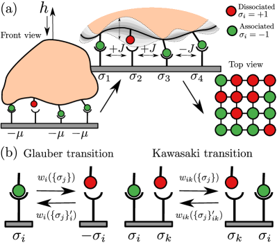
Figure 1: A coarse-grained model for the cooperative association/dissociation of adhesion bonds. (a) Schematic of the effective many-body model governed by Eq. (1) and (2), depicting an adhesion domain on a cell-patch with 16 CAMs anchored to stiff substrate. Adhesion bonds are arranged on a $4\times 4$ square lattice and can assume two states, $\sigma_{i}=\pm 1$, where $+1$ corresponds to an open (red) and $-1$ to a closed bond (green). Nearest-neighbor bonds experience an effective interaction $J$ induced by undulations of the anchoring membrane. An external force $h$ is pulling/pushing on the adhesion domain. Each adhesion bond has an intrinsic binding-affinity $\mu\geq 0$ that favors a bound state. A small number of bonds is depicted for convenience only. In the work we consider different system sizes including the thermodynamic limit. (b) Glauber and Kawasaki transition. A Glauber transition changes the binding state of a single adhesion bond to $\sigma_{i}\rightarrow-\sigma_{i}$ with transition rate $w_{i}(\{\sigma_{j}\})$ (see Eq. (3)). A Kawasaki transition interchanges two nearest-neighbor adhesion bonds $\sigma_{i}\leftrightarrow\sigma_{k}$ with transition rate $w_{ik}(\{\sigma_{j}\})$ (see Eq. (5)), corresponding to lateral diffusion.

Most of our current understanding of the formation and stability of adhesion clusters derives from the analysis of individual [11] and non-interacting adhesion bonds [62, 63, 64], and studies of collective effects in biomimetic vesicular model systems with floppy membranes [65, 48] and mobile CAMs [66]. These results therefore do not necessarily apply to cells, where membranes are stiffened by the presence of, and receptors are anchored to, the stiff actin cytoskeleton that can actively exert forces on the membrane [9].

Notwithstanding all theoretical efforts [15, 16, 17, 43, 18, 49, 19, 44, 46, 47], a consistent and comprehensive physical picture of collective adhesion under the action of a mechanical force that could explain the observations on live cellular systems [56, 57, 58, 41, 3, 59, 67, 60] remains elusive. For example, whether the coupling of individual bonds causes the collective association and dissociation rates to increase or decrease, respectively, was speculated to depend on the intrinsic single-bond affinity [21, 68], cell type (i.e. surface corrugation) [39] and on the state of the actin cytoskeleton [21]. An understanding of cellular adhesion therefore must integrate the complex interplay between the correlated, collective (un)binding [18, 41, 46, 47, 48, 49, 65], the intrinsic affinity of anchored adhesion bonds [21, 68, 69], the cell type and surface topology [39], as well as the integrity of, and forces generated by, the actin cytoskeleton [21, 34, 57, 58, 59] under physiological [67] or pathological conditions [70, 71, 60, 72].

While it is omnipresent in biological systems, cell adhesion displays subtle differences in the specific microsopic details. Here we aim to capture the essential general features of the physics of cell adhesion. In order to arrive at a deeper understanding of the mechanical regulation of cellular adhesion that would explain the collective dynamics of adhesion bonds on the level of individual (un)binding events we here consider mixed Glauber-Kawasaki dynamics of a generic, two-dimensional model of diffusing nearest-neighbor interacting adhesion bonds with intrinsic affinity $\mu$ under the action of a shared force $h$ (see Fig. 1a).

Highly accurate analytical results on the Bethe-Guggenheim level reveal the many-body (that is, beyond “mean field”) physics underlying biological adhesion. We consider in detail cluster-sizes ranging from a few CAMs to the thermodynamic limit. In the thermodynamic limit we determine the equation of state and complete phase behavior that displays a phase separation and co-existence of dense and dilute adhesion domains. The critical behavior is investigated in detail and striking differences are found between pulling- and pushing-forces. Strikingly, we prove the existence of a seemingly new kind of dynamical phase transition – the mean first passage time to cluster formation/dissolution is proven to change discontinuously with respect to the coupling strength. This dynamical phase transition, and more generally the non-linear and non-monotonic dependence on the membrane flexibility, may explain the puzzling cooperative behavior of effective association and dissociation rates measured experimentally.

I.1 Outline of the work

The paper is structured as follows. In Sec. II we present an effective mesoscopic model of adhesion clusters and provide a practical roadmap to the diverse calculations and analyses. In Sec. III we present explicit analytical results for the thermodynamic equation of state and complete phase behavior of adhesion clusters, and in Sec. IV we present analytical results for the kinetics of cluster formation and dissolution both in the presence and absence of forces. In Sec. V we discuss the biological implications of our results and in particular the suggestive rôle of criticality in the context of equilibrium adhesion strength and the kinetic dissolution and formation rates, respectively. Finally, in Sec. VI we highlight the relevance of our results in the context of the Ising model. We conclude in Sec. VII with a summary and a perspective on the importance and limitations of our results, and mention possible extensions to be made in future studies. Details of calculations, explicit asymptotic results and further technical information is presented in a series of Appendices.

II Model of interacting adhesion bonds under shared force

II.1 Equilibrium

We consider a two-dimensional patch of a cell surface with $N$ adhesion molecules embedded in the cell membrane, their lateral positions forming a lattice with coordination number $z$ (see Fig. 1). The results we derive hold for any lattice but we focus the discussion mainly on the square lattice with free boundary conditions. Opposing the patch is a stiff substrate or a neighboring cell-patch with complementary adhesion molecules occupying a commensurate lattice. The state of individual bonds is denoted by $\sigma_{i}$, $i=1,2,...,N$, where $\sigma_{i}=+1$ if bond $i$ is broken an $\sigma_{i}=-1$ if it is closed.

In the presence of a timescale separation the opening/closing of nearest neighbor bonds is coupled via membrane fluctuations. Following closely the arguments of Ref. [17] we can integrate out the membrane degrees of freedom to obtain an effective Ising-like model for the bonds within the patch with effective Hamiltonian

$$\mathcal{H}(\{\sigma_{i}\})=-J\sum_{\langle ij\rangle}\sigma_{i}\sigma_{j}-\mu N_{c}(\{\sigma_{i}\})+\mathcal{H}_{\rm h}(\{\sigma_{i}\}),$$ (1)

where $J\geq 0$ is the membrane-induced short-range coupling between the bonds, $\langle ij\rangle$ denotes all nearest-neighbor pairs, $\mu$ is the effective chemical potential (i.e. intrinsic affinity) of individual bonds, and $\mathcal{H}_{\rm h}(\{\sigma_{i}\})$ is the Hamiltonian describing the effect of the mechanical force. The first term in Eq. (1) represents the effective coupling between nearest neighbor bonds, and is isomorphic to the interaction term in the Ising model [73]. It is an effective measure of bond-cooperativity, i.e. it reflects that the (free) energy penalty of closing/breaking a bond is smaller if neighboring bonds are closed/open, respectively [17]. Such an effective description in terms of bonds coupled via a short-range membrane-mediated interaction is feasible when bonds are flexible and/or the patch of the cell membrane is quite (but not completely) stiff and is thus rather pulled down as a whole instead of being locally strongly deformed by the binding of individual bonds [17]. In this limit the coupling strength is determined by the effective bending rigidity of the cell membrane, $\kappa$, via $J\propto 1/\sqrt{\kappa}$ (see [17] and Appendix A). That is, in this regime a relatively floppier cell membrane with lower bending rigidity induces a stronger cooperativity between neighboring bonds than a relatively stiff membrane. Notably, a detailed comparison between the full model of specific adhesion (i.e. reversible adhesion bonds explicitly coupled to a dynamic fluctuating membrane) and the lattice model captured by the first term of Eq. (1) revealed a quantitative agreement (see e.g. Fig. 5 in [17]) in the range $0\leq J\lesssim 1.2\,k_{\rm B}T$ that lies entirely within the rather stiff limit [17]. This is the range of $J$ we are interested in and includes the values relevant for cell adhesion (see Sec. V below).

The second term in Eq. (1) reflects that each closed bond stabilizes the adhesion cluster by an amount $-\mu$. Aside from the last term $\mathcal{H}_{\rm h}(\{\sigma_{i}\})$ the Hamiltonian (1) is isomorphic to the lattice gas model developed in [17], and a mapping between the two models is provided in Appendix A.

The third term in Eq. (1), $\mathcal{H}_{\rm h}(\{\sigma_{i}\})$, accounts for the mechanical force $h$ acting on the membrane-embedded bonds that we assume to be equally shared between all $N_{c}$ closed bonds of a given configuration $\{\sigma_{i}\}$, i.e. $N_{c}(\{\sigma_{i}\})\equiv\sum_{i}\delta_{\sigma_{i},-1}$, where $\delta_{ik}$ is Kronecker’s delta. More precisely, the force $h$ destabilizes the bound state by introducing an elastic (free) energy penalty on all closed bonds whereby broken bonds remain unaffected. If all bonds are closed, $N_{c}=N$, this penalty is set to be $hx_{0}$, where $x_{0}$ is a microscopic length-scale specific for a given CAM that merely sets the energy scale associated with the elastic strain caused by $h$. Conversely, the penalty must vanish in a completely dissolved configuration with $N_{c}=0$, and is assumed to be a smooth and monotonic function of $N_{c}$. A mathematically and physically consistent definition is

$$\mathcal{H}_{\rm h}(\{\sigma_{i}\})=-2hx_{0}\left(\frac{1}{1+N_{c}(\{\sigma_{i}\})/N}-1\right).$$ (2)

A ’pulling force’, $h>0$, favors the dissociation of bonds while a ’pushing force’, $h<0$, favors their association. We are interested in strain energies on the order of the thermal energy per bond, i.e. $|h|x_{0}/N=\mathcal{O}(k_{\rm B}T)$. Note that the assumption of an equally shared force in Eq. (2) is valid if either of the following conditions is satisfied: the anchoring membrane has a large combined elastic modulus (i.e. stiff membranes or membrane/substrate pairs), individual bonds are flexible, the bond-density is low, or the membrane is prestressed by the actin cytoskeleton [74, 43, 75]. In the limit of a rather stiff membrane both, a spin representation with effective coupling $J$ and a uniform force load are valid approximations to describe cell adhesion under force over a broad range of physically relevant parameters, as we detail below. The implications of a non-uniform force load are addressed in detail in Sec. VII and Appendix E.2.

II.2 Kinetics

The breaking/closure and lateral diffusion of adhesion bonds are assumed to evolve as a discrete time Markov chain with mixed single-bond-flip Glauber dynamics [76] and two-bond-exchange Kawasaki dynamics [77] (see Fig. 1b). For a single jump in the Markov chain we define the probability to attempt a Glauber transition as $p_{k}\in[0,1]$ which controls the diffusion rate, and for the sake of generality is allowed to depend on the number of closed bonds $k$. Similarly, the probability to attempt a Kawasaki transition is given by $1-p_{k}\in[0,1]$. We consider two distinct scenarios, one in which adhesion bonds are immobile due to being anchored to the underlying cytoskeleton (i.e. $p_{k}=1\ \forall k$), and the other in which adhesion molecules are allowed to transiently diffuse (i.e. $0<p_{k}<1\ \forall k$; see e.g. [10]). Conversely, permanently associated/dissociated freely diffusing bonds (i.e. $p_{k}=0\ \forall k$) will not be considered, since these are not relevant. Further details about the respective transition rates are given below.

Glauber transitions: Let $\{\sigma_{j}\}^{\prime}_{i}$ denote the bond configuration obtained by flipping bond $i$ while keeping the configuration of all other bonds fixed, i.e. $\{\sigma_{j}\}^{\prime}_{i}\equiv(-\sigma_{i},\{\sigma_{j\neq i}\})$. Moreover, let $w_{i}(\{\sigma_{j}\})$ denote the transition rate from $\{\sigma_{j}\}$ to $\{\sigma_{j}\}^{\prime}_{i}$ and $\Delta\mathcal{H}_{i}(\{\sigma_{j}\})\equiv\mathcal{H}(\{\sigma_{j}\}_{i}^{\prime})-\mathcal{H}(\{\sigma_{j}\})$ the energy difference associated with the transition. These rates can be specified uniquely by limiting interactions to nearest-neighbors, imposing isotropy in position space, and requiring that $w_{i}$ satisfies detailed balance, i.e. $w_{i}(\{\sigma_{j}\})/w_{i}(\{\sigma_{j}\}_{i}^{\prime})=\exp{(-\beta\Delta\mathcal{H}_{i}(\{\sigma_{j}\}))}$, where $\beta=1/k_{\mathrm{B}}T$ is the inverse thermal energy. The general result reads $w_{i}(\{\sigma_{j}\})=\alpha[1-\tanh(\beta\Delta\mathcal{H}_{i}(\{\sigma_{j}\})/2)]/2N$, where $\alpha$ is an intrinsic attempt-frequency that sets the fastest timescale [76], and time will throughout be expressed in units of $\alpha^{-1}$. Introducing furthermore the dimensionless quantities $\tilde{J}=\beta J$, $\tilde{\mu}=\beta\mu$ and $\tilde{h}=\beta hx_{0}/N$ this leads to

$$w_{i}(\{\sigma_{j}\})=\frac{\alpha}{2N}\bigg{\{}1-\sigma_{i}\tanh\!\Big{[}\tilde{J}\sum_{\langle ij\rangle}\!\sigma_{j}-\frac{\tilde{\mu}}{2}\!+\!\Lambda^{\tilde{h}}_{\{\sigma_{j}\},i}\Big{]}\bigg{\}},$$ (3)

where we defined the auxiliary function

$$\Lambda^{\tilde{h}}_{\{\sigma_{j}\},i}\equiv\frac{\tilde{h}}{(1+N_{c}(\{\sigma_{j}\})/N)(1+N_{c}(\{\sigma_{j}\}^{\prime}_{i})/N)}.$$ (4)

Kawasaki transitions: Let $\{\sigma_{j}\}^{\prime}_{ik}$ denote the bond configuration upon interchanging the state of the nearest neighbor bonds $\sigma_{i}$ and $\sigma_{k}$ while keeping the configuration of all other bonds fixed, i.e. $\{\sigma_{j}\}^{\prime}_{ik}\equiv(\sigma_{i}\leftrightarrow\sigma_{k},\{\sigma_{j\neq(i,k)}\})$. We denote the Kawasaki transition rate from $\{\sigma_{j}\}$ to $\{\sigma_{j}\}^{\prime}_{ik}$ as $w_{ik}(\{\sigma_{j}\})$, where $\Delta\mathcal{H}_{ik}(\{\sigma_{j}\})\equiv\mathcal{H}(\{\sigma_{j}\}_{ik}^{\prime})-\mathcal{H}(\{\sigma_{j}\})$ is the energy difference associated with the transition. Imposing the same symmetry constraints as for the Glauber rates as well as detailed-balance yields the general expression [77]

$$w_{ik}(\{\sigma_{j}\})=\frac{\alpha}{2N}\bigg{\{}1-\frac{\sigma_{i}-\sigma_{k}}{2}\tanh\!\Big{[}\tilde{J}(\sum_{\langle ij\rangle}\sigma_{j}-\sum_{\langle kl\rangle}\sigma_{l})\Big{]}\bigg{\}},$$ (5)

where we have used that $(\sigma_{i}-\sigma_{k})/2\in\{-1,0,1\}$. As pointed out in [77], the transition is only meaningful when $\sigma_{k}=-\sigma_{i}$, otherwise the transition brings the system to an identical state, which is equivalent to no transition. Note that the Kawasaki rates given by Eq. (5) do not depend on the external force $\tilde{h}$ nor the binding-affinity $\tilde{\mu}$, since the Kawasaki transition conserves the total number of open and closed adhesion bonds. However, if in addition we introduce a position-dependent force/binding affinity the Kawasaki rates also depend on $\tilde{h}$ and $\tilde{\mu}$, which we analyze in Appendix E.2.

II.3 Strategy roadmap

We focus in detail on both, the equilibrium properties as well as the kinetics of cluster formation and dissolution for all cluster sizes. A roadmap to our extensive analysis is presented in Fig. 2.

For small to moderate cluster sizes, i.e. up to $50$ bonds for the equilibrium properties and up to $25$ bonds in the case of formation/dissolution kinetics, we obtain exact solutions using standard algebraic methods [78]. To circumvent the explosion of combinatorial complexity for large system sizes we employ a variational approach – the so-called Bethe-Guggenheim approximation [79] – to derive closed-form expressions for the partition function, and finally carry out the thermodynamic limit to derive explicit closed-form results for large adhesion clusters. When considering the formation/dissolution kinetics of large clusters and in particular in the thermodynamic limit, we employ the local equilibrium approximation, where we assume that the growth and dissolution evolves like a birth-death process on the free energy landscape.

We systematically test the accuracy of all approximations by comparing them with exact results for system sizes that are amenable to exact solutions. The results reveal a remarkable accuracy that improves further with the size of the system (e.g. see Fig. B1).

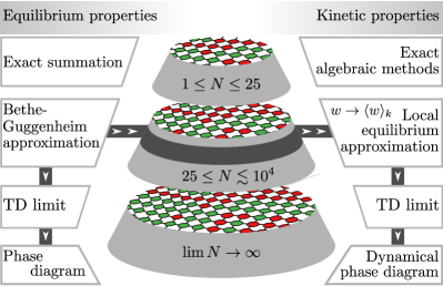
Figure 2: Strategy roadmap. Small system sizes $N\leq 5\times 5$ are solved for exactly. The thermodynamics of larger systems is treated on the level of the highly accurate Bethe-Guggenheim approximation and the kinetics by assuming local equilibrium. Within the Bethe-Guggenheim approximation we take the thermodynamic (TD) limit $N\to\infty$ and determine the phase behavior, master scaling of dissolution/formation kinetics and analyze the statical and dynamical critical behavior.

III Equilibrium behavior of adhesion clusters

III.1 Small and intermediate clusters

In order to quantify the equilibrium stability of adhesion clusters we first analyze the equation of state for the average fraction of closed bonds, $\langle\varphi\rangle\equiv\langle N_{c}(\{\sigma_{i}\})\rangle/N$ at given $\tilde{\mu},\tilde{J}$ and $\tilde{h}$. To this end we require $Q_{k}$, the partition function constrained to the number of closed bonds $N_{c}(\{\sigma_{i}\})=k$. We therefore write the total canonical partition function $Q$ for a system of $N$ adhesion bonds as $Q\equiv\sum_{\{\sigma_{i}\}}\mathrm{e}^{-\beta\mathcal{H}(\{\sigma_{i}\})}\equiv\sum_{k=0}^{N}Q_{k}$, where

$$Q_{k}\equiv\sum_{\{\sigma_{i}\}}\mathrm{e}^{-\beta\mathcal{H}(\{\sigma_{i}\})}\delta_{N_{c}(\{\sigma_{i}\}),k}=\mathrm{e}^{[\tilde{\mu}+2\tilde{h}(k/N+1)^{-1}]k}Z_{k},$$ (6)

and $Z_{k}\equiv\sum_{\{\sigma_{i}\}}\exp{(\tilde{J}\sum_{\langle ij\rangle}\sigma_{i}\sigma_{j})}\delta_{N_{c}(\{\sigma_{i}\}),k}$ is the partition function of the Ising model at zero field conditioned to have a magnetization $N/2-k$. The free energy density (per bond) in units of thermal energy $k_{\rm B}T$ constrained to a given fraction of closed bonds $\varphi$, $\tilde{f}_{N}(\varphi)$, and the equation of state, $\langle\varphi(\tilde{\mu},\tilde{J},\tilde{h})\rangle$, are given by

$$\tilde{f}_{N}(\varphi)=-N^{-1}\ln Q_{k},\quad\langle\varphi\rangle=N^{-1}\partial_{\tilde{\mu}}\ln Q.$$ (7)

We note that $\mathrm{e}^{-N\tilde{f}_{N}(\varphi)}/Q={\rm Prob}(N_{c}=N\varphi)$ in an equilibrium ensemble of $N$ bonds. The sum over constrained configurations in $Z_{k}$ contains $\binom{N}{k}$ terms. Whereas it can be performed exactly for $N\lesssim 50$ it explodes for larger system sizes. To overcome the computational complexity we employ a variational approach – the Bethe-Guggenheim approximation [79], yielding (see derivation in Appendix B.1)

$$Z_{k}\approx Z^{\mathrm{BG}}_{k}=\binom{N}{k}\frac{\psi_{\bar{z}N}^{\bar{z}k}(\bar{z}X_{k}^{*})}{\psi_{\bar{z}N}^{\bar{z}k}(\bar{z}\bar{X}_{k})}\mathrm{e}^{-\bar{z}\tilde{J}(2\bar{X}_{k}-N/2)},$$ (8)

where $\bar{z}=\sum_{i=1}^{N}z_{i}/N$ is the average coordination number in a cluster with local coordination $z_{i}$ that accounts for finite-size effects, $X_{k}^{*}\equiv k(N-k)/N$, we have defined

$$\bar{X}_{k}\equiv\frac{2X_{k}^{*}}{[1+4X_{k}^{*}(\mathrm{e}^{4\tilde{J}}-1)/N]^{1/2}+1},$$ (9)

and introduced the auxiliary function

$$\psi_{a}^{b}(x){\equiv}\Gamma([b-x]/2+1)\Gamma^{2}(x/2+1)\Gamma([a-b-x]/2+1),$$ (10)

where $\Gamma(z)$ stands for the Gamma function. Note that by setting $\bar{X}_{k}=X_{k}^{*}$ in Eq. (8) we recover the mean field result $Z_{k}^{\rm MF}$ (which happens automatically for $\tilde{J}=0$ or $k=0\lor N$) which is discussed in Appendix C.1.

Fig. 3(a-c) shows a comparison of the free energy density $\tilde{f}_{N}(\varphi)$ for a cluster of $40$ bonds for various affinities $\tilde{\mu}$ and external forces $\tilde{h}$, and confirms the high accuracy of the Bethe-Guggenheim approximation on the one hand, and the systematic failure of the mean field result on the other hand. This signifies that correlations between adhesion bonds decisively affect cluster properties. Moreover, pairwise correlations captured by the Bethe-Guggenheim approach are apparently dominant, whereas three-body and higher order correlations that were ignored are apparently insignificant.

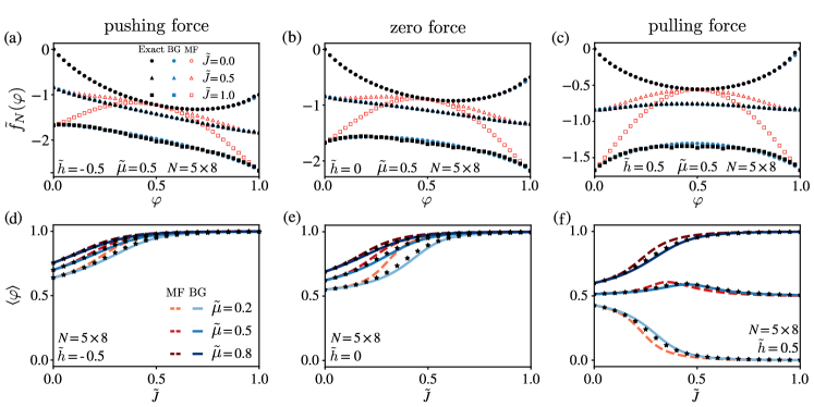
Figure 3: Free energy landscape and equation of state for small clusters. (a-c) Free energy density conditioned on $\varphi$, $\tilde{f}_{N}(\varphi)$ from Eq. (7) for a system of $N=5\times 8$ bonds on a square lattice for (a) a pushing force $\tilde{h}=-0.5$, (e) no force $\tilde{h}=0$, and (f) pulling force $\tilde{h}=0.5$; Black symbols depict exact results, blue symbols the Bethe-Guggenheim approximation, and red symbols the mean field result. (d-f) Equation of state, $\langle\varphi\rangle$, for a cluster of $5\times 8$ adhesion bonds on a square lattice as a function of the dimensionless coupling $\tilde{J}$ for (d) a pushing force $\tilde{h}=-0.5$, (e) no force and (f) a pulling force $\tilde{h}=0.5$. Symbols depict exact results, blue lines correspond to the Bethe-Guggenheim approximation and red to the mean field result.

Similarly, in Fig. 3(d-f) we depict the equation of state for a cluster of 40 bonds. The Bethe-Guggenheim approximation (blue lines) is very accurate for all values of $\tilde{J}$ whereas the mean field approximation (red lines) fails for intermediate values of the coupling. We observe striking differences in the dependence of $\langle\varphi\rangle$ on the coupling $\tilde{J}$ (and hence membrane rigidity) with respect to the intrinsic binding-affinity $\tilde{\mu}$ in the presence of a pulling force (see Fig. 3f). At strong coupling between adhesion bonds $\langle\varphi\rangle$ depends strongly on $\tilde{\mu}$. In the presence of a pulling force adhesion bonds with a weak affinity are on average all broken, whereas they are all closed if the affinity is large. Notably, the dependence of $\langle\varphi\rangle$ on the coupling $\tilde{J}$ at zero force (see Fig. 3e) agrees qualitatively well with experimental observations [21, 68, 39, 21] and hints at some form of critical behavior underneath, which we discuss in more detail in Sec. V.

III.2 Thermodynamic limit

To explore the phase diagram in detail and analyze the critical behavior we consider the thermodynamic limit of the Bethe-Guggenheim (BG) and mean field (MF) free energy density, i.e. the scaling limit

$$\tilde{\rm f}^{\rm BG,MF}(\varphi)\equiv\lim_{\begin{subarray}{c}N\to\infty,\\ k/N=\varphi={\rm const.}\end{subarray}}\tilde{f}^{\rm BG,MF}_{N}(\varphi),$$ (11)

which exists and is given by

$$\tilde{\rm f}^{\rm BG}(\varphi)=-\tilde{\mu}\varphi+2\tilde{h}\frac{\varphi}{1+\varphi}+\frac{1}{2}\tilde{J}\bar{z}[4\Omega_{\varphi}-1]+\frac{\bar{z}}{2}[\Xi(\varphi-\Omega_{\varphi})+\Xi(1-\varphi-\Omega_{\varphi})+2\Xi(\Omega_{\varphi})]+(1-\bar{z})[\Xi(\varphi)+\Xi(1-\varphi)],$$ (12)

where $X_{\varphi}^{*}/N=\varphi(1-\varphi)$, $\Omega_{\varphi}\equiv\bar{X}_{\varphi}/N$, and we have introduced the auxiliary function $\Xi(x)\equiv x\ln x$. The result for $\tilde{\rm f}^{\rm MF}(\varphi)$ is given in Appendix C.1. Somewhat surprisingly the free energy density of a finite system, $\tilde{f}_{N}^{\rm BG}(\varphi)$, converges to the thermodynamic limit $\tilde{\rm f}^{\rm BG}(\varphi)$ already for $N\gtrsim 100$. For convenience we henceforth drop the superscript BG when considering the Bethe-Guggenheim result, i.e. $\tilde{\rm f}^{\rm BG}(\varphi)\to\tilde{\rm f}(\varphi)$.

The equation of state in the thermodynamic limit is determined by means of the saddle-point method (for derivation see Appendix D), yielding a weighted sum over $\varphi^{0}_{i}$, the $M$ global minima of $\tilde{\rm f}(\varphi)$:

$$\langle\varphi\rangle_{\rm TD}=\lim_{N\to\infty}N^{-1}\partial_{\tilde{\mu}}\ln Q^{\rm BG}\simeq\sum_{i=1}^{M}c_{i}\varphi^{0}_{i},$$ (13)

where $\tilde{\rm f}(\varphi_{i}^{0})=\tilde{\rm f}_{\rm min},\forall i$, and $\simeq$ stands for asymptotic equality in the thermodynamic limit. In practice $M$ is either 1 (unique minimum) or 2 (two-fold degenerate minima). The minima have the universal form $\varphi^{0}_{m}=\xi_{\tilde{\mu},\tilde{J},\tilde{h}}^{4}/(1+\xi_{\tilde{\mu},\tilde{J},\tilde{h}}^{4})$ with the coefficients $\xi_{\tilde{\mu},\tilde{J},\tilde{h}}$ and weights $c_{i}$ given explicitly in Appendix D.

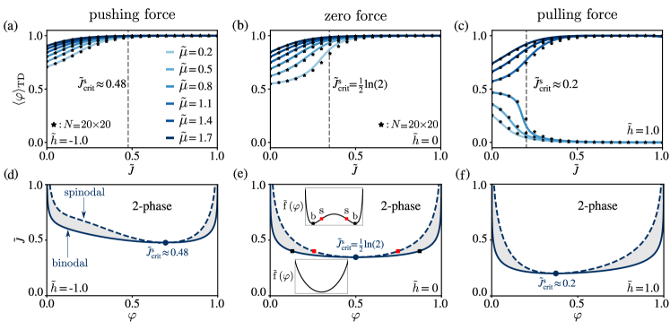
Figure 4: Equation of state and phase diagram in the thermodynamic limit. (a-c) $\langle\varphi\rangle$ for a cluster of $20\times 20$ adhesion bonds on a square lattice (symbols) and the saddle-point asymptotic $\langle\varphi\rangle_{\rm TD}$ from Eq. (13) as a function of the dimensionless coupling $\tilde{J}$ for various affinities $\tilde{\mu}$ and for (a) a pushing force $\tilde{h}=-1$, (b) no force, and (c) a pulling force $\tilde{h}=1$. The dashed vertical line denotes the (statical) critical coupling strength $\tilde{J}^{s}_{\rm crit}$ whereupon the system phase-separates into dense and dilute phases of closed bonds. (d-e) Phase diagram for (d) a pushing force $\tilde{h}=-1$, (e) no force, and (f) a pulling force $\tilde{h}=1$; the full and dashed lines depict the binodal and spinodal line, respectively. The shaded area depicts the region where the system is metastable. The blue circle depicts the (statical) critical point $(\varphi^{s}_{\rm crit},\tilde{J}^{s}_{\rm crit})$. Inset in (e): Schematic of the free energy landscape $\tilde{\rm f}(\varphi)$ below the critical coupling $\tilde{J}<\tilde{J}^{s}_{\rm crit}$ (bottom) displaying a single minimum, and a bi-stable free energy landscape above the critical coupling $\tilde{J}>\tilde{J}^{s}_{\rm crit}$ (top), with the black and red symbols illustrating the meaning of phase compositions highlighted in the phase diagram.

The equation of state $\langle\varphi\rangle$ for a finite cluster seems to converge to the saddle-point asymptotic $\langle\varphi\rangle_{\rm TD}$ already for $N\gtrsim 400$ for any value of the force $\tilde{h}$, bond affinity $\tilde{\mu}$, and coupling $\tilde{J}$ (see Fig. 4(a-c)), and is qualitatively the same as for smaller clusters (compare Fig. 4(a-c) with Fig. 3(d-f)). However, important differences emerge in the thermodynamic limit – the system may undergo a phase transition and phase-separate into dense (“liquid”) and dilute (“gas”) phases of closed bonds with composition $\varphi_{l}$ and $\varphi_{g}$, respectively (see also [49]).

III.3 Phase diagram and critical behavior

To determine the phase diagram we require the binodal $\tilde{J}_{b}(\varphi)$ and spinodal $\tilde{J}_{s}(\varphi)$ line. The binodal line $\tilde{J}_{b}(\varphi)$ denotes the onset of phase separation and is determined by the “common tangent” construction, i.e. from the solution of the coupled equations

$$\tilde{\rm f}^{\prime}(\varphi_{l})=\tilde{\rm f}^{\prime}(\varphi_{g}),\quad\frac{\tilde{\rm f}(\varphi_{l})-\tilde{\rm f}(\varphi_{g})}{\varphi_{l}-\varphi_{g}}=\tilde{\rm f}^{\prime}(\varphi_{l}),$$ (14)

where the prime denotes the derivative with respect to $\varphi$ at constant $\tilde{J}$. The spinodal line $\tilde{J}_{s}(\varphi)$, also known as the stability boundary, denotes the boundary between the metastable and unstable regimes and is determined by $\tilde{\rm f}^{\prime\prime}(\varphi)=0$. For a non-zero force, $\tilde{h}\neq 0$, we determine $\tilde{J}_{b}(\varphi)$ numerically, whereas we obtain an exact result for a vanishing force $\tilde{h}=0$ that reads (see derivation in Appendix B.2)

$$\tilde{J}_{b}(\varphi,\tilde{h})|_{\tilde{h}=0}=\frac{1}{2}\ln\left(\frac{1-\chi_{\varphi}}{\chi_{\varphi}^{1/\bar{z}}-\chi_{\varphi}^{1-1/\bar{z}}}\right),$$ (15)

where we have introduced $\chi_{\varphi}=\varphi/(1-\varphi)$. The spinodal line for any force $\tilde{h}$ is in turn given exactly by

$$\tilde{J}_{s}(\varphi,\tilde{h})=\frac{1}{4}\ln\left\{\frac{[\varphi-\Phi(\varphi,\tilde{h})][1-\varphi-\Phi(\varphi,\tilde{h})]}{\Phi(\varphi,\tilde{h})^{2}}\right\},$$ (16)

with the auxiliary function

$$\Phi(\varphi,\tilde{h})\equiv 2\varphi(1-\varphi)+\bar{z}\left[\frac{1-\bar{z}}{\varphi(1-\varphi)}-\frac{4\tilde{h}}{(1+\varphi)^{3}}\right]^{-1},$$ (17)

that is defined for $(2-\bar{z})/8\tilde{h}\leq\varphi(1-\varphi)/(1+\varphi)^{3}\leq(1-\bar{z})/4\tilde{h}$. Note that it follows from their respective definitions that neither $\tilde{J}_{b}(\varphi,\tilde{h})$ nor $\tilde{J}_{s}(\varphi,\tilde{h})$ depends on $\tilde{\mu}$ (for a proof see Appendix B.2). The phase diagram for a pushing, zero, and pulling force $\tilde{h}$ is shown in Fig. 4(d-f) and displays, above the critical coupling strength $\tilde{J}>\tilde{J}^{s}_{\rm crit}$, a phase separation into a dense and dilute phase of closed bonds with compositions $\varphi_{l}$ and $\varphi_{g}$, respectively. A pushing force $\tilde{h}<0$ lifts the critical coupling and “tilts” the phase diagram towards higher density, i.e. at a given coupling $\tilde{J}>\tilde{J}^{s}_{\rm crit}$ the density of both phases increases. Conversely, a pulling force $\tilde{h}>0$ lowers the critical coupling and “tilts” the phase diagram towards lower density, i.e. at a given coupling $\tilde{J}>\tilde{J}^{s}_{\rm crit}$ the density of both phases decreases. The biological implications of these results will be discussed in Sec. V. The binodal and spinodal line in the mean field approximation are given in Appendix C.2.

We now address in detail the behavior of the statical critical point $(\varphi^{s}_{\rm crit},\tilde{J}^{s}_{\rm crit})$ – the point where the binodal and spinodal merge, $\tilde{J}_{b}(\varphi^{s}_{\rm crit},\tilde{h})=\tilde{J}_{s}(\varphi^{s}_{\rm crit},\tilde{h})\equiv\tilde{J}^{s}_{\rm crit}(\varphi^{s}_{\rm crit},\tilde{h})$. The critical point denotes the onset of phase separation and is the solution of $\tilde{\rm f}^{\prime\prime\prime}(\varphi)=0$, which in absence of the force yields (for derivation see Appendix B.2) $(\varphi^{s,0}_{\rm crit},\tilde{J}^{s,0}_{\rm crit})\equiv\frac{1}{2}(1,\ln\frac{\bar{z}}{\bar{z}-2})$. In the presence of a force $\tilde{h}\neq 0$ we obtain the exact solution using a Newton’s series approach [80, 81, 82] (for details regarding the Newton series, see Appendix D.2). The analytical result is non-trivial and is given explicitly in Appendix B.2. For small forces $|\tilde{h}|\ll 1$ we in addition derive a second order perturbation expansion $\tilde{J}^{s}_{\rm crit}=\tilde{J}^{s,0}_{\rm crit}-\delta\tilde{J}^{s}_{\rm crit}(\tilde{h})+\mathcal{O}(\tilde{h}^{3})$, where

$$\delta\tilde{J}^{s}_{\rm crit}(\tilde{h})=\frac{8}{27}\frac{1}{\bar{z}-2}\left(\tilde{h}+\frac{2}{27}\frac{\bar{z}+2}{\bar{z}-1}\tilde{h}^{2}\right),$$ (18)

and correspondingly $\varphi^{s}_{\rm crit}=\varphi^{s,0}_{\rm crit}-\delta\varphi_{\rm crit}(\tilde{h})+\mathcal{O}(\tilde{h}^{3})$ with

$$\delta\varphi_{\rm crit}(\tilde{h})=\frac{2}{3}\frac{(\bar{z}/3)^{2}}{(\bar{z}-2)(\bar{z}-1)}\left[\tilde{h}+\frac{16}{9}\frac{(\bar{z}/3)^{2}-\bar{z}+1}{(\bar{z}-2)(\bar{z}-1)}\tilde{h}^{2}\right].$$ (19)

The dependence of the statical critical point on the external force is depicted in Fig. 5. A pulling force (red) pulls the critical point towards lower $\tilde{J}$ and lower $\varphi$, whereas a pushing force (blue) effects the opposite and shifts the critical point towards larger coupling $\tilde{J}$ and higher density $\varphi$. The mean field statical critical point can be derived exactly as a function of the force $\tilde{h}$, and the result is given in Appendix C.2.

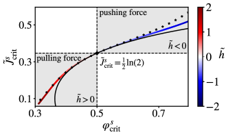
Figure 5: Statical critical point as a function of the force $\tilde{h}$. Symbols depict the exact solution using a converged Newton’s series and the gradient line depicts the two-term (so-called quadratic) approximation of the complete Newton’s series, which is very accurate for any pulling- and up to a moderate pushing force, i.e. $\tilde{h}\geq-1$. Explicit expressions are given in Appendix E. The black line corresponds to the prediction of second order perturbation theory from Eqs. (18) and (19) that is valid for small forces.

IV Kinetics of cluster formation and dissolution

IV.1 Small and intermediate clusters

We are interested in the kinetics of cluster formation from a completely unbound state, and cluster dissolution from a completely bound state. More general initial conditions are treated in Appendix E. We quantify the kinetics by means of the mean first passage time $\langle\tau_{d,f}\rangle$, where the subscripts $d$ and $f$ stand for dissolution and formation, respectively, and $\tau_{d,f}$ is the first passage time defined as

$$\tau_{d} \equiv \inf_{t}\left[\varphi(\{\sigma_{i}\}_{t})=0|\varphi(\{\sigma_{i}\}_{0})=1\right],$$

$$\tau_{f} \equiv \inf_{t}\left[\varphi(\{\sigma_{i}\}_{t})=1|\varphi(\{\sigma_{i}\}_{0})=0\right],$$ (20)

where $\{\sigma_{i}\}_{t}$ denotes the instantaneous state at time $t$. A cluster with $N$ adhesion bonds has $2^{N}$ possible states $\{\sigma_{i}\}$. We enumerate them such that the first state corresponds to all bonds closed and the final state to all bonds broken. The transition matrix of the Markov chain describing mixed Glauber-Kawasaki dynamics on this state-space has dimension $2^{N}\times 2^{N}$, whereby we must impose absorbing boundary conditions on the fully dissolved and fully bound states, respectively. An exact algebraic result for $\langle\tau_{d,f}\rangle$ is given in Eq. (E2) in Appendix E.1 but requires the inversion of a $(2^{N}-1)\times(2^{N}-1)$ sparse matrix, followed by a sum over $2^{N}-1$ terms, which is feasible only for $N\lesssim 5\times 5$.

As a result of the non-systematic cluster formation and dissolution at zero coupling $\tilde{J}=0$, and motivated by the intuitive idea that the dynamics is dominated by low energy (i.e. minimum action) paths at large coupling $\tilde{J}\gg 1$, we make the so-called local equilibrium approximation to treat large clusters. Thereby we map the dynamics of the $2^{N}\times 2^{N}$ state-space onto a one-dimensional birth-death process for the instantaneous number of closed bonds $k$ (see Fig. 6) with effective transition rates

$$\bar{w}_{k\to k\pm 1}\equiv\tilde{Q}^{-1}_{k}\sum_{\{\sigma_{i}\}}\mathrm{e}^{-\beta\mathcal{H}(\{\sigma_{i}\})}w^{\pm}_{\rm exit}(\{\sigma_{i}\})\delta_{N_{c}(\{\sigma_{i}\}),k},$$ (21)

where we have defined the re-weighted canonical partition function $\tilde{Q}_{k}\equiv Q_{k}/p_{k}$ where $p_{k}$ is the Glauber attempt probability in state $k$, and we have introduced the exit rates from configuration $\{\sigma_{i}\}$ in the “$+$” (i.e. $N_{c}(\{\sigma_{i}\}^{\prime}_{j})=N_{c}(\{\sigma_{i}\})+1$) and “$-$” (i.e. $N_{c}(\{\sigma_{i}\}^{\prime}_{j})=N_{c}(\{\sigma_{i}\})-1$) direction, respectively, given by

$$w^{\pm}_{\rm exit}(\{\sigma_{i}\})\equiv\sum_{j=1}^{N}w_{j}(\{\sigma_{i}\})\delta_{N_{c}(\{\sigma_{i}\}^{\prime}_{j}),k\pm 1}.$$ (22)

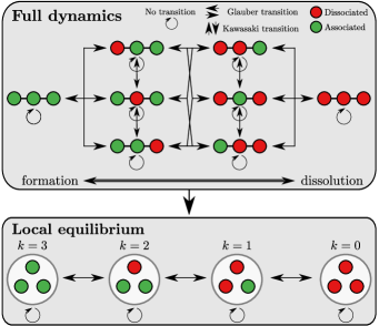
Figure 6: Mapping the full dynamics onto a birth-death process. For convenience, and without any loss of generality, we here show an example of a system composed of 3 adhesion bonds on a 1-dimensional lattice. The mapping holds for any lattice geometry. In the full dynamics each lattice configuration represents a different node, comprising a $2^{N}\times 2^{N}$ transition matrix, whereas in the local equilibrium approximation we only need to distinguish between states with a different number of closed/open bonds, comprising a $(N+1)\times(N+1)$ transition matrix.

Note that only the Glauber transitions, given by Eq. (3), enter in Eq. (22). The Kawasaki transitions given by Eq. (5), which conserve the total number of closed bonds, enter the dynamics through the diagonal of the transition matrix as the waiting rates $\bar{w}_{k\rightarrow k}=1-\bar{w}_{k\rightarrow k+1}-\bar{w}_{k\rightarrow k-1}$, where the right hand side follows from conservation of probability. Within the local equilibrium approximation the mean first passage time for cluster dissolution and formation become, respectively

$$\langle\tau_{d}\rangle\approx\langle\tau_{d}^{\rm le}\rangle = \sum_{k=0}^{N-1}\frac{1}{\bar{w}_{k\to k+1}}\sum_{l=k+1}^{N}\frac{\tilde{Q}_{l}}{\tilde{Q}_{k}}$$

$$\langle\tau_{f}\rangle\approx\langle\tau_{f}^{\rm le}\rangle = \sum_{k=1}^{N}\frac{1}{\bar{w}_{k\to k-1}}\sum_{l=0}^{k-1}\frac{\tilde{Q}_{l}}{\tilde{Q}_{k}},$$ (23)

where one can further use the detailed balance relation $\tilde{Q}_{k}\bar{w}_{k\to k-1}=\tilde{Q}_{k-1}\bar{w}_{k-1\to k}$ (which we prove in Appendix E.3) to interchange the backward and forward rate in the second line and change the summation according to $\sum_{k=1}^{N}\bar{w}_{k\to k-1}^{-1}\sum_{l=0}^{k-1}\tilde{Q}_{l}/\tilde{Q}_{k}\to\sum_{k=0}^{N-1}\bar{w}_{k\to k+1}^{-1}\sum_{l=0}^{k}\tilde{Q}_{l}/\tilde{Q}_{k}$. In Appendix E.4 we prove that Eq. (23) holds for any birth-death process where the transition rates obey detailed balance. A comparison of the exact result given by Eq. (E2) with the local equilibrium approximation in Eq. (23) shown in Fig. 7 demonstrates the remarkable accuracy of the approximation already for $N\sim 20$ bonds, which increases further for larger $N$. The reason for the high accuracy can be found in the large entropic barrier to align bonds in an unbound/bound state, effecting a local equilibration prior to complete formation/dissolution. Moreover, the local equilibrium approximation is expected to become asymptotically exact even for small clusters in the ideal, non-interacting limit $\tilde{J}\to 0$ as well as for $\tilde{J}\to\infty$ that is dominated by the minimum-action, “instanton” path. A further discussion of the local equilibrium approximation and an approximate closed form expression for Eq. (23) for larger systems is given in Appendices E.5 and E.6.

Figure 7: Kinetics of dissolution and formation of small clusters. Mean first passage time for cluster dissolution (a) and formation (b) as a function of the coupling $\tilde{J}$ for $N=4\times 5$ adhesion bonds with intrinsic affinity $\tilde{\mu}=0.5$ in the absence of a force (for nonzero force values see Fig E3). Colored lines correspond to exact results obtained from Eq. (E2) for various values of the Glauber attempt probability $p$, which we set to be constant $p_{k}\rightarrow p$, and symbols denote the local equilibrium approximation Eq. (23) evaluated with the exact $Q_{k}$ and $\bar{w}_{k\to k\pm 1}$ from Eqs. (6) and (21) respectively.

The mean first passage times for cluster dissolution/formation shown in Fig. 7 both display a strong and non-monotonic dependence on the coupling parameter $\tilde{J}$ with a pronounced minimum, hinting at some form of critical dynamics. As we prove below this minimum in the thermodynamic limit indeed corresponds to a dynamical critical coupling.

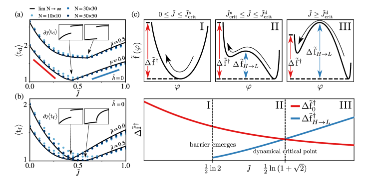
Figure 8: Master scaling of mean dissolution and formation times per bond for finite clusters and in the thermodynamic limit, and the origin of the dynamical critical point. $\langle{\rm t_{d,f}}\rangle$ for cluster dissolution (a) and formation (b) as a function of the coupling $\tilde{J}$ for a pair of intrinsic affinities $\tilde{\mu}=0$ and $\tilde{\mu}=0.5$ and various cluster sizes (symbols) as well as the thermodynamic limit (lines) in the absence of an external force; Symbols are evaluated with local equilibrium approximation Eqs. (23) using $Q_{k}^{\rm BG}$ (Eqs. (6) and (8)) and $\bar{w}_{k\to k+1}$ from Eq. (21). The discrepancy between the lines and symbols is due to finite-size effects. (c) In the thermodynamic limit and more generally for large clusters the mean dissolution/formation time $\langle{\rm t_{d,f}}\rangle$ depends only on the largest free energy barrier (see Eq. (24)). For small coupling (regime I) the latter corresponds to the difference between the free energy minimum and the fully dissolved or bound configuration, $\Delta\tilde{\rm f}^{\dagger}=\Delta\tilde{\rm f}^{\dagger}_{0,1}$, respectively. At the statical critical coupling value, $J^{s}_{\rm crit}$, (onset of regime II) a free energy barrier emerges separating the meta-stable from the stable phase, $\Delta\tilde{\rm f}^{\dagger}_{H\rightleftarrows L}$, but the largest free energy barrier is still $\Delta\tilde{\rm f}^{\dagger}=\Delta\tilde{\rm f}^{\dagger}_{0,1}$. At the dynamical critical coupling, $\tilde{J}^{d}_{\rm crit}$, (onset of regime III) the free energy barrier separating the meta-stable from the stable phase becomes dominant, $\Delta\tilde{\rm f}^{\dagger}=\Delta\tilde{\rm f}^{\dagger}_{H\rightleftarrows L}$. The depicted free energy landscapes $\tilde{\rm f}(\varphi)$ correspond to Eq. (12) with $\tilde{\mu}=0.05$ and $\tilde{h}=0$.

IV.2 Thermodynamic limit

We now consider dissolution and formation kinetics in very large clusters, i.e. in the limit $N\to\infty$. Note that while the mean first passage time formally diverges, i.e. $\lim_{N\to\infty}\langle\tau_{d,f}\rangle=\infty$, it is expected to do so in a “mathematically nice”, well-defined “bulk scaling”. In anticipation of an exponential scaling of relevant time-scales with the system size $N$ we define the mean formation/dissolution time per bond in the thermodynamic limit as $\langle{\rm t_{d,f}}\rangle\equiv\lim_{N\to\infty}\langle\tau_{d,f}\rangle^{1/N}$. Using the local equilibrium approximation for the mean first passage time given by Eq. (23), and assuming that the Glauber attempt probabilities $p_{k}$ are strictly sub-exponential in $N$, we prove via a squeezing theorem in Appendix E.7 that the exact mean dissolution and formation time per bond in the thermodynamic limit reads

$$\langle{\rm t_{d,f}}\rangle=\mathrm{e}^{\tilde{\rm f}(\varphi^{d,f}_{\rm max})-\tilde{\rm f}(\varphi^{d,f}_{\rm min})}\equiv\mathrm{e}^{\Delta\tilde{\rm f}^{\dagger}},$$ (24)

where

$$\varphi^{d}_{\rm max} \equiv \sup_{\varphi<1}\tilde{\rm f}(\varphi),\quad\varphi^{d}_{\rm min}\equiv\inf_{\varphi>\varphi^{d}_{\rm max}}\tilde{\rm f}(\varphi),$$

$$\varphi^{f}_{\rm max} \equiv \sup_{\varphi>0}\tilde{\rm f}(\varphi),\quad\varphi^{f}_{\rm min}\equiv\inf_{\varphi<\varphi^{f}_{\rm max}}\tilde{\rm f}(\varphi).$$ (25)

Eq. (24) shows that the mean first passage per bond in the thermodynamic limit is determined exactly by the largest left/right-approaching free energy barrier between the initial and final point, and is completely independent of the Glauber attempt probability $p_{k}$. We obtain analytical results for Eqs. (24) and (25) for arbitrary $\tilde{J},\tilde{\mu}$ and $\tilde{h}$. Since these results are somewhat complicated for $\tilde{\mu}>0$ and $\tilde{h}\neq 0$ we present them in Appendix E.8 and Fig E4. In the force-free case with zero intrinsic affinity, i.e. $\tilde{\mu}=\tilde{h}=0$, they turn out to be surprisingly compact and given by

$$\langle{\rm t_{d,f}}\rangle=\left\{\begin{array}[]{lc}2\mathrm{e}^{-2\tilde{J}}\cosh^{2}\tilde{J},&0\leq\tilde{J}\leq\frac{1}{2}\ln{2}\\ \displaystyle{4\frac{\sinh^{2}2\tilde{J}}{\mathrm{e}^{4\tilde{J}}-2}},&\frac{1}{2}\ln{2}\leq\!\tilde{J}\!\leq\frac{1}{2}\ln{(1\!+\!\sqrt{2})}\\ \displaystyle{8\mathrm{e}^{2\tilde{J}}\frac{\sinh^{2}\tilde{J}}{\mathrm{e}^{4\tilde{J}}-2}},&\tilde{J}\geq\frac{1}{2}\ln{(1\!+\!\sqrt{2})},\end{array}\right.$$ (29)

such that for $\tilde{J}=0$ and $\tilde{J}\to\infty$ we have $\langle{\rm t_{d,f}}\rangle=2$ being the maximum, and the minimum occurs at $\tilde{J}=\ln{(1+\sqrt{2})}/2$ where $\langle{\rm t_{d,f}}\rangle=(4/7)(2\sqrt{2}-1)$. Fig. 8a,b shows a comparison of the prediction of Eq. (24) with the results for finite system given by Eqs. (23) and (21) rescaled according to $\langle\tau_{d,f}\rangle^{1/N}$. Already for $N=900$ a nearly complete collapse to the thermodynamic limit (24) is observed for both, cluster formation as well as dissolution. The mean field analogue of Eq. (29) is given by Eq. (E35) for a general $\bar{z}$ and remarkably has a universal (i.e. $\bar{z}$-independent) minimum value of $\langle{\rm t_{d,f}}\rangle_{\rm MF}\approx 1.0785$ at the dynamical critical coupling $\tilde{J}=2\ln{(2)}/\bar{z}$ (see Eq. (E37)). Moreover, $\langle{\rm t_{d,f}}\rangle_{\rm MF}$ displays an unphysical divergence in the limit $\tilde{J}\to\infty$ (see Fig. E5).

IV.3 Dynamical phase transition and critical behavior

Strikingly, the mean dissolution and formation time in the thermodynamic limit (24) display a discontinuity as a function of the coupling $\tilde{J}$ (see jumps in $\partial_{\tilde{J}}\langle{\rm t_{d,f}}\rangle$ depicted in the insets in Fig. 8a,b). In particular, for zero affinity and external force we find from Eq. (29)

$$\lim_{\tilde{J}\nearrow\frac{1}{2}\ln(1+\sqrt{2})}\partial_{\tilde{J}}\langle{\rm t_{d,f}}\rangle = -(4/7)^{2}(13\sqrt{2}-17)$$

$$\lim_{\tilde{J}\searrow\frac{1}{2}\ln(1+\sqrt{2})}\partial_{\tilde{J}}\langle{\rm t_{d,f}}\rangle = (8/7^{2})(9\sqrt{2}-8).$$

This implies the existence of a first order dynamical phase transition at the dynamical critical coupling $\tilde{J}^{d}_{\rm crit}$ and hence a qualitative change in the dominant dissolution/formation pathway. Coincidentally, the Bethe-Guggenheim dynamical critical point for $\tilde{\mu}=\tilde{h}=0$ coincides with the exact (Onsager’s) statical critical point for the two-dimensional zero-field Ising model [83]. Similarly, the mean field dynamical critical point for $\tilde{\mu}=\tilde{h}=0$ coincides with the Bethe-Guggenheim statical critical point (for a more detailed discussion see Appendices E.8 and E.9). Strikingly, the dynamic critical point always corresponds to the minimum of $\langle{\rm t_{d,f}}\rangle$. The explanation of the physics underneath the dynamical phase transition and the meaning of $\tilde{J}^{d}_{\rm crit}$ is given in Fig. 8c.

The qualitative behavior of $\langle{\rm t_{d,f}}\rangle$ has three distinct regimes. In regime I, where $0\leq\tilde{J}<\tilde{J}^{s}_{\rm crit}$, the free energy landscape $\tilde{\rm f}(\varphi)$ has a single well and according to Eq. (24) $\langle{\rm t_{d,f}}\rangle$ is determined by $\Delta\tilde{\rm f}^{\dagger}_{0,1}$ – the free energy difference between the minimum and the absorbing point (i.e. $\varphi=0$ for dissolution and $\varphi=1$ for formation, respectively). $\Delta\tilde{\rm f}^{\dagger}_{0,1}$ is a decreasing function of $\tilde{J}$.

At the statical critical coupling $\tilde{J}^{s}_{\rm crit}$, which marks the onset of regime II, a second free energy barrier emerges delimiting the phase-separated low ($L$) and a high ($H$) density phase. We denote this free energy barrier by $\Delta\tilde{\rm f}^{\dagger}_{H\rightleftarrows L}$ where $\rightarrow$ and $\leftarrow$ stand for dissolution and formation, respectively. $\Delta\tilde{\rm f}^{\dagger}_{H\rightleftarrows L}$ is an increasing function of $\tilde{J}$. In regime II, that is when $\tilde{J}^{s}_{\rm crit}\leq\tilde{J}<\tilde{J}^{d}_{\rm crit}$, the dissolution and formation first evolve through a (thermodynamic) phase transition and, finally, must also surmount the second, predominantly entropic barrier to the complete dissolved/bound state. In regime II, as in regime I, the largest free energy barrier remains the free energy difference between the minimum and the absorbing point, i.e. $\Delta\tilde{\rm f}^{\dagger}_{0,1}>\Delta\tilde{\rm f}^{\dagger}_{H\rightleftarrows L}$.

Exactly at the dynamical critical coupling $\tilde{J}^{d}_{\rm crit}$ the two barriers become identical, $\Delta\tilde{\rm f}^{\dagger}_{0,1}=\Delta\tilde{\rm f}^{\dagger}_{H\rightleftarrows L}$ and for $\tilde{J}>\tilde{J}^{d}_{\rm crit}$ we always have $\Delta\tilde{\rm f}^{\dagger}_{0,1}<\Delta\tilde{\rm f}^{\dagger}_{H\rightleftarrows L}$. Therefore, in regime III the rate-limiting event becomes the phase transition itself, whereas the fully dissolved/bound state is thereupon reached by typical density fluctuations. Since $\Delta\tilde{\rm f}^{\dagger}_{0,1}$ decreases with $\tilde{J}$ while $\Delta\tilde{\rm f}^{\dagger}_{H\rightleftarrows L}$ increases with $\tilde{J}$, the mean dissolution/formation time per bond at the dynamical critical coupling $\tilde{J}^{d}_{\rm crit}$ must be minimal. This explains the dynamical phase transition completely.

Note that the dynamical phase transition is preserved under initial conditions that lie beyond the largest free energy barrier (from the final/absorbing state). For example, we may consider $\varphi(\{\sigma_{i}\}_{0})=\varphi_{L,H}^{0}$ in Eq. (20), where $\varphi_{L,H}^{0}$ is the (meta)-stable minimum in the high and low density region for cluster dissolution and formation, respectively. In the thermodynamic limit the equilibration time from the initial condition $\varphi(\{\sigma_{i}\})=0\lor 1$ to the (meta)-stable minimum $\varphi_{L,H}^{0}$ becomes exponentially faster than the total transition time, which renders $\langle{\rm t}_{\rm d,f}\rangle$ unaffected.

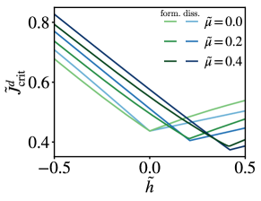
Figure 9: Dynamical critical point. Dynamical critical coupling $\tilde{J}^{d}_{\rm crit}$ as a function of the external force $\tilde{h}$ for several values of the intrinsic binding-affinity $\tilde{\mu}$. Note that $\tilde{J}^{d}_{\rm crit}$ as a function of $\tilde{h}$ may be non-monotonic with a global minimum whose location depends on $\tilde{\mu}$.

The dependence of $\tilde{J}^{d}_{\rm crit}$ on $\tilde{\mu}$ and $\tilde{h}$ is determined in the form of a Newton’s series in Appendix  E.8, and is depicted in Fig. 9. Depending on the intrinsic affinity $\tilde{\mu}$, the dependence of $\tilde{J}^{d}_{\rm crit}$ may be non-monotonic. Note that in contrast to the statical critical coupling $\tilde{J}^{\rm s}_{\rm crit}$ that is independent of $\tilde{\mu}$, the dynamical critical coupling $\tilde{J}^{\rm d}_{\rm crit}$ depends on the particular value of $\tilde{\mu}$.

V Many-body physics in the mechanical regulation of adhesion

Our results tie the effective bending rigidity, $\kappa$, and in turn interactions between neighboring adhesion bonds, $\tilde{J}\propto\kappa^{-1/2}$ (see Appendix A), to the collective phase behavior of adhesion clusters at equilibrium, and to distinct dynamical phases of cluster dissolution and formation. Based on the quantitative relationship between the coupling strength $\tilde{J}$ and bending ridigity $\kappa$ given by Eq. (A3), and an order-of-magnitude estimation of the relevant parameters listed in Table 1 we find that the coupling strength in cellular systems lies within the range $0\lesssim\tilde{J}\lesssim 2.5$. Notably, both the statical and dynamical critical point at moderate values of the external force values and/or intrinsic binding-affinity lie within said range (see Fig. 5 and 9). Yet, it remains to be explained why a near-critical coupling may be beneficial for cells, and how it may be regulated.

Table 1: Estimated parameter values in cellular systems.

Estimated parameter values
Parameter	Symbol	Estimated value / range	Source
Spring constant	$\beta k$	$\sim 10^{-2}\ \ [{\rm nm}^{-2}]$	[84, 85, 17]
Non-specific interaction strength	$\beta\gamma$	$\sim 10^{-5}\ \ [{\rm nm}^{-4}]$	[17]
Bond separation distance	$h_{0}-l_{0}$	$25\sim 50\ \ \ \ [{\rm nm}]$	[84, 86, 87]
Bending rigidity	$\beta\kappa$	$4\sim 400$	[88, 89, 90, 55]

Our results provoke the hypothesis that the membrane rigidity (and hence the coupling strength) may lie close to the statical critical value for quasi-static, and near the dynamical critical value for transient processes. Mechanical regulation of the bending rigidity can be achieved through hypotonic swelling [91], (de)polymerization of the F-actin network [92, 93], by decoupling the F-actin network from the plasma membrane [55], through changes of the membrane composition [94, 95, 88, 89] or integral membrane proteins [95], membrane-protein activity [96], temperature modulation [35, 88, 28], and acidosis [45], to name but a few. Moreover, it has been shown experimentally that temperature modulations affects adhesion strength through changes in membrane fluidity [28], cell elasticity [35], or via a temperature cooperative process [26], albeit the denaturation of the binding proteins also provides a possible explanation [36].

Below we argue that the change in the response of a cell to a perturbation, defined as a change in the equilibrium binding strength or association/dissociation rates, is largest near criticality. This results in either a very small or very large response, depending on the change of the underlying parameter. Here we follow the same kind of reasoning as rooted in the criticality hypothesis, which states that systems undergoing an order–disorder phase transition achieve the highest trade-off between robustness an flexibility around criticality [97].

V.1 Criticality at equilibrium

In Fig. 10a we depict how oscillations in the coupling strength (arising through oscillations in the bending rigidity $\kappa$) around the statical critical point affect the average fraction of closed bonds. Similar oscillatory patterns and their effect on the adhesion strength have been observed in vascular smooth muscle cells, where changes in the bending rigidity were concerted by the remodeling of the actin cytoskeleton [57, 58, 34]. Minute changes in the amplitude, $\delta\tilde{J}$, can drive the systems’s behavior from oscillations within a dense phase with $\langle\varphi(t)\rangle>0.5$ to intermittent periods of nearly complete dissolution (compare full and dashed lines in Fig. 10a). Hence we find that the response (i.e. $\langle\varphi(t)\rangle$) is most sensitive to a change in the amplitude $\delta\tilde{J}$ when $\tilde{J}$ lies close to the statical critical point.

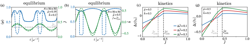
Figure 10: Equilibrium and kinetic response to changes in cell stiffness, external force, or the binding-affinity. Equilibrium response of the average fraction of closed bonds $\langle\varphi(t)\rangle$ to a slow (quasi-static), periodic modulation of (a) the coupling $\tilde{J}(t)=\tilde{J}+\delta\tilde{J}\sin(\omega t)$ (and hence membrane stiffness) and (b) the external force $\tilde{h}(t)=\tilde{h}+\delta\tilde{h}\sin(\omega t)$. Note the strong sensitivity of the response near the statical critical coupling $\tilde{J}^{s}_{\rm crit}$. (c-d) Change in mean dissolution (c) and formation (d) time per bond, $\Delta_{\tilde{J}}\langle{\rm t_{d,f}}\rangle\equiv\langle{\rm t_{d,f}}(\tilde{J}+\Delta\tilde{J})\rangle-\langle{\rm t_{d,f}}(\tilde{J})\rangle$, as a response to a change $\Delta\tilde{J}$ of the coupling, as a function of $\tilde{J}$ for various $\Delta\tilde{J}$. The kinetic response is largest for $\tilde{J}$ near the dynamical critical coupling.

Similarly, in Fig. 10b we show the response of $\langle\varphi(t)\rangle$ to a mechanical perturbation oscillating quasi-statically between a pulling and a pushing force, $\tilde{h}(t)=\tilde{h}_{\rm ref}+\delta\tilde{h}\sin(\omega t)$ (for practical examples see e.g. [98, 99]). Such mechanical perturbations can for example arise through changes in active stresses generated within the cytoskeleton [100]. Here as well, a small change in the force $\delta\tilde{h}$ acting on the cluster, can lead to stark differences in the cluster stability $\langle\varphi(t)\rangle$. The sensitivity to a change in the the force is most amplified near the statical critical coupling $\tilde{J}^{s}_{\rm crit}$ (compare full and dashed lines in Fig. 10b), where a small change in the amplitude, $\delta\tilde{h}$, can cause intermittent periods of essentially complete cluster detachment.

Drastic changes in the average number of closed bonds have been observed experimentally in adhesion frequency assays and single-molecule microscopy [21, 68]. There it was shown that binding affinities and binding dynamics for a T-cell receptor (TCR) interacting with the peptide-major histocompatbility complex (pMHC) are more than an order of magnitude smaller in solution (i.e. in 3D) as compared to when they are anchored to a cell membrane (i.e. in 2D). One possible contribution to the discrepancy between the 3D and 2D binding kinetics is the difference in the reduction of the entropy upon binding, which is larger in 3D than in 2D [40]. However, it has been explicitly remarked that this contribution alone does not explain the measured difference in the binding affinities [40]. The authors of Ref. [21, 68] rationalize these differences in binding in terms of a cooperativity between neighboring TCRs due to the anchoring membrane. In particular, Fig. 11a in the Supplementary Material of Ref. [68] shows the adhesion frequency $P_{a}(t_{\rm c})\in[0,1]$, defined as the fraction of observed adhesion events between the TCR and pMHC as a function of the contact time $t_{\rm c}$ between the anchoring membranes, derived from Monte-Carlo simulations. Upon introducing a heuristic neighbor-dependent amplification factor in the binding rates the authors observe an amplification of the adhesion frequency $P_{a}$ (compare squares with diamonds), indicating an increase in binding events in agreement with their experimental observations.

We may relate our results to the observations in Ref. [68] by recalling the relation between $P_{a}$ and $\langle N_{c}\rangle=N\langle\varphi\rangle$, i.e. $P^{\rm ss}_{a}\equiv\lim_{t_{\rm c}\rightarrow\infty}P_{a}(t_{\rm c})=1-\exp{(-N\langle\varphi\rangle)}$ (see [101] as well as Eqs. (1) and (2) in [68]). In our model the aforementioned amplification factor arises naturally from a nonzero coupling strength $\tilde{J}$ due to the anchoring membrane. Indeed, in Fig. 3e an increase in $\tilde{J}$ leads to an increase in $\langle\varphi\rangle$, which in turn causes an increase of the steady state adhesion frequency $P^{\rm ss}_{a}$. Hence we find that the amplification factor in [68] and coupling $\tilde{J}$ in our model have the same effect on the adhesion frequency.

A similar observation was made in [39] on the basis of a detailed analysis of the binding affinities of the adhesion receptor CD16b placed in three distinct environments: red blood cells (RBCs), detached Chinese hamster ovary (CHO) cells, and K562 cells. Based on Fig. 4a,b in [39] the adhesion frequency for RBCs is around a 15-fold larger than for CHO and K562 cells. In the discussion the authors point towards the modulation of surface smoothness as an explanation for the observed differences in adhesion frequency [39]. Since K562 cells are known to have a larger bending rigidity than RBCs [102, 103] (we were unfortunately not able to find the corresponding information for CHO cells in the existing literature), it is expected that the coupling strength $\tilde{J}$ is generally higher in the latter (see Appendix A), which provides a potential explanation for the observed difference in adhesion frequencies between RBCs and K562 cells.

V.2 Criticality in kinetics

Many biological processes [104, 105, 106, 107] and experiments [108, 109, 110] involve adhesion under transient, non-equilibrium conditions, where cells can become detached completely from a substrate (for a particular realization with a constant force see [108]). The duration of these transients may be quantified by the mean dissolution and formation time, $\langle{\rm t_{d,f}}\rangle$ (see Fig. 8). Imagine that the cell can change the bending rigidity by an amount $\Delta\kappa$ that in turn translates into a change in coupling, $\tilde{J}^{\prime}=\tilde{J}+\Delta\tilde{J}\propto 1/\sqrt{\kappa+\Delta\kappa}$. If the mechanical regulation is to be efficient, a small change of $\Delta\tilde{J}$ should effect a large change of $\langle{\rm t_{d,f}}\rangle$.

The efficiency of the regulation, expressed as the change of mean dissolution/formation time in response to a change $\Delta\tilde{J}$, $\Delta\langle{\rm t_{d,f}}\rangle\equiv\langle{\rm t_{d,f}}(\tilde{J}+\Delta\tilde{J})\rangle-\langle{\rm t_{d,f}}(\tilde{J})\rangle$, is shown in Fig. 10(c-d). The results demonstrate that the regulation is most efficient, that is gives the largest change, when $\tilde{J}$ is poised near the dynamical critical coupling, $\tilde{J}\simeq\tilde{J}^{d}_{\rm crit}$, regardless of the magnitude of the change $\Delta\tilde{J}$. Recall that the formation and dissolution rate, $1/\langle{\rm t_{f}}\rangle$ and $1/\langle{\rm t_{d}}\rangle$, respectively, are highest at the dynamical critical coupling (see Fig. 8). Therefore not only do we find the largest response to a change in $\tilde{J}$, but also the fastest formation and dissolution kinetics at the dynamical critical coupling $\tilde{J}\simeq\tilde{J}^{d}_{\rm crit}$.

An example where fast kinetic (un)binding and a large sensitivity to the bending rigidity can be beneficial is found in tumor cells that undergo metastasis - the process through which tumor cells spread to secondary locations in the host’s body. Recent studies suggest that cancer cells are mechanically more compliant than normal, healthy cells [111]. Moreover, experiments with magnetic-tweezers have shown that membrane stiffness of patient tumor cells and cancer cell-lines inversely correlates with their migration and invasion potential [60], and an increase of membrane rigidity alone is sufficient to inhibit invasiveness of cancer cells [90]. Cells with the highest invasive capacity were found to be five times less stiff than cells with the lowest migration and invasion potential, but the underlying mechanism behind this correlation remained elusive [60].

Based on our results a decrease in the bending rigidity, and hence the membrane stiffness, can alter both, the equilibrium strength of adhesion (see Fig. 3) as well as the kinetics of formation and dissolution of adhesion domains (see Fig. 8). This may provide a clue about the mechanical dysregulation of cell adhesion in metastasis in terms of a softening of the cell membrane.

VI Criticality in the Ising model

By setting $\tilde{h}=0$ and writing $\delta_{\sigma_{j},-1}=(1-\sigma_{j})/2$ we find that Eq. (1) is, up to a constant, identical to the Hamiltonian of the isotropic ferromagnetic Ising model in a uniform external magnetic field $M\equiv\mu/2$. Therefore, our findings, and in particular the uncovered dynamical phase transition, also provide new insight into equilibrium and kinetic properties of the Ising model in the presence of a uniform external magnetic field.

The equilibrium properties of the two-dimensional Ising model in the absence of a magnetic field, such as the total free energy per spin, statical critical point, and binodal line were obtained in the seminal work by Onsager [83]. The effect of a uniform magnetic field has mostly been studied numerically [112, 113], e.g. by Monte-Carlo simulations [114] and renormalization group theory [115], but hitherto no exact closed-form expression for the free energy per spin has been found. On the Bethe-Guggenheim level the free energy density, binodal line, spinodal line, and statical critical point were known [116], but to our knowledge we are the first to provide an exact closed-form expression for the equation of state in the presence of a uniform magnetic field (see Appendix D).

The kinetics of the two-dimensional Ising model have been studied in the context of magnetization-reversal times (i.e. the time required to reverse the magnetization) [117, 118, 119], nucleation times [120, 121], and critical slowing down [122, 123]. Here we report a new type of dynamical critical phenomenon related to a first-order discontinuity and a global minimum of the magnetization reversal time at the concurrent dynamical critical point (see Fig. 8), which is fundamentally different from the statical critical point. The dynamical phase transition reflects a qualitative change in the instanton path towards magnetization reversal, and has not been reported before.

In Table 2 we summarize the values of the statical and dynamical critical points obtained by the mean field and Bethe-Guggenheim approximation in the absence of a magnetic field, and for a general coordination number $\bar{z}$ (for a derivation of the dynamical critical points see Appendices E.8 and E.9). We also state the exact statical critical point of the two-dimensional Ising model. Conversely, the exact dynamical critical point of the two-dimensional Ising model remains unknown as it requires the exact free energy density as a function of the fraction of down spins (see Eq. (12) for the result within the Bethe-Guggenheim approximation). A lower bound on the dynamical critical point is set by the statical critical point, as the latter denotes the onset of an interior local maximum that is required for the dynamical critical point (see Fig. 8). The exact dynamical critical point may provide further insight into the nature of the dynamical phase transition. Moreover, it also sets a lower bound on the magnetization reversal times per spin in ferromagnetic systems in the absence of an external force.

Table 2: Statical and dynamical critical point as a function of the coordination number $\bar{z}$ obtained within the mean field and Bethe-Guggenheim approximation, alongside the exact statical critical point $\tilde{J}^{\rm s}_{\rm crit}$ for the two-dimensional Ising model at zero field and binding-affinity, $\tilde{\mu}=\tilde{h}=0$. The exact dynamical critical point $\tilde{J}^{\rm d}_{\rm crit}$ for the two-dimensional Ising model remains unknown; a lower bound is given by the Onsager statical critical point.

Critical points
Approximation	$\tilde{J}^{s}_{\rm crit}$	$\tilde{J}^{d}_{\rm crit}$
Mean field	$\frac{1}{\bar{z}}$	$\frac{2}{\bar{z}}\ln{2}$
Bethe-Guggenheim	$\frac{1}{2}\ln{\left(\frac{\bar{z}}{\bar{z}-2}\right)}$	$\frac{-1}{2}\ln{(2^{1-2/\bar{z}}-1)}$
Exact 2D	$\frac{1}{2}\ln{\left(1+\sqrt{2}\right)}$	$\geq\tilde{J}^{s}_{\rm crit}$

VII Concluding remarks

The behavior of individual [11] and non-interacting [62, 63, 74, 64] adhesion bonds under force, the effect of the elastic properties of the substrate and pre-stresses in the membrane [43, 75], as well as the physical origin of the interaction between opening and closing of individual adhesion bonds due to the coupling with the fluctuating cell membrane [15, 16, 17, 18, 19, 124, 44, 46, 125] are by now theoretically well established. However, in order to understand the importance of these interactions and their manifestation for the mechanical regulation of cell adhesion in and out of equilibrium one must go deeper, and disentangle the response of adhesion clusters of all sizes to external forces and how it becomes altered by changes in membrane stiffness. This is paramount because interactions strongly change the physical behavior of adhesion clusters under force both, qualitatively as well as quantitatively.

Founded on firm background knowledge [11, 62, 63, 74, 64, 43, 75, 15, 16, 17, 18, 19, 124, 44, 46, 125] our explicit analytical results provide deeper insight into cooperative effects in cell-adhesion dynamics and integrate them into a comprehensive physical picture of cell adhesion under force. We considered the full range of CAM binding-affinities and forces, and established the phase behavior of two-dimensional adhesion clusters at equilibrium as well as the kinetics of their formation and dissolution.

We have obtained, to the best of our knowledge, the first theoretical results on equilibrium behavior and dynamic stability of adhesion clusters in the thermodynamic limit beyond the mean field-level (existing studies, even those addressing non-interacting adhesion bonds [63, 74, 64], are limited to small clusters sizes [43, 75, 16, 17, 18]). We explained the complete thermodynamic phase behavior, including the co-existence of dense and dilute adhesion domains, and characterized in detail the corresponding critical behavior.

We demonstrated conclusively the existence of a seemingly new kind of dynamical phase transition in the kinetics of adhesion cluster formation and dissolution, which arises due to the interactions between the bonds and occurs at a critical coupling $\tilde{J}^{d}_{\rm crit}$, whose value depends on the external force $\tilde{h}$ and binding-affinity $\tilde{\mu}$. At the dynamical critical coupling $\tilde{J}^{d}_{\rm crit}$, and in turn critical bending rigidity $\kappa^{d}_{\rm crit}\propto(\tilde{J}^{d}_{\rm crit})^{-2}$, the dominant formation and dissolution pathways change qualitatively. Below $\tilde{J}^{d}_{\rm crit}$ the rate-determining step for cluster formation and dissolution is the surmounting of the (mostly) entropic barrier to completely bound and unbound states, respectively. Conversely, above $\tilde{J}^{d}_{\rm crit}$ the thermodynamic phase transition between the dense and dilute phase for dissolution, and between the dilute and dense phase for cluster formation, becomes rate-limiting, whereas the completely bound and unbound states, respectively, are thereupon reached by typical density fluctuations.

We expect the non-monotonic dependence of the mean first passage time to cluster dissolution/formation on the coupling strength $\tilde{J}$ that is asymmetric around the minimum to be experimentally observable (though the notion of a fully bound state during cluster formation may be experimentally ambiguous). According to our theory the existence of such a minimum and its asymmetric shape would immediately imply a dynamical phase transition in the thermodynamic limit.
Measuring the mean dissolution/formation time (in the absence or presence of an external force) for an ensemble of cells adhering to a stiff substrate seems to be experimentally feasible. The effective membrane rigidity (and thus the coupling $\tilde{J}$) could in principle be controlled by varying the membrane composition (e.g. increasing the cholesterol concentration that in turn increases membrane rigidity [88]), by tuning the osmotic pressure of the medium [126], or by the depolymerization of F-actin [127]. Testing for signatures of the theoretically predicted dynamical phase transition thus seems to be experimentally (at least conceptually) possible, and we hope that our results will motivate such investigations.

We discussed the biological implications of our results in the context of mechanical regulation of the bending rigidity around criticality. Based on our results we have suggested that the response of a cell to a change in the bending rigidity may be largest near the statical critical point for quasi-static processes, and near the dynamical critical point for transient processes. This observation agrees with the criticality hypothesis, and might expand the list of biological processes hypothesized to be poised at criticality [128].

Finally, we discussed the implications of our result for the two-dimensional Ising model. The observed dynamical phase transition is related to a first-order discontinuity in the magnetization reversal time, and the exact dynamical critical point for the two-dimensional Ising model remains elusive (see Table 2).

We now remark on the limitations of our results. The mapping onto a lattice gas/Ising model (i.e. Eq. (1) and Appendix A; see also [16, 17]) may not apply to genuinely floppy membranes encountered in biomimetic vesicular systems [65, 48]. Moreover, since we only allow for two possible states of the bonds, i.e. associated and dissociated, we neglect any internal degrees of freedom (e.g. orientations of the bonds) which may contribute to the entropy loss upon binding [40], thereby changing the free energy.

Likewise, the assumption of an equally shared force is generally good for stiff membranes (stiffened by the presence of, or anchoring to, the stiff actin cytoskeleton [9]) or stiff membrane/substrate pairs, flexible individual bonds, low bond-densities, or the presence of pre-stresses exerted by the actin cytoskeleton [74, 43, 75]. In Appendix E.2 we provide an analysis of the effect of a non-uniform force load. Based on this analysis we find that in the case of rather floppy membranes, corresponding to large values of the coupling strength $\tilde{J}=\mathcal{O}(1)$, the difference between a uniform and a non-uniform force load is negligible for a broad range of realizations of the non-uniform force distribution. Only under the extreme, non-physiological condition that the ratio of forces experienced by inner and outer bonds is larger than an order of magnitude, we observe significant differences. Therefore, the dependencies of the statical and dynamical critical points on the external force (see Figs. 5 and 8, respectively) are expected to remain valid for a non-uniform force distribution over a large range of force magnitudes.

In their present form our results may not apply to conditions when cells actively contract in response to a mechanical force on a timescale comparable to cluster assembly or dissolution [129], as well as situations in which cells actively counteract the effect of an external pulling force and make adhesion clusters grow (see results in terms of a change in membrane stiffness as well.

Finally, throughout we have considered clusters consisting of so-called “slip-bonds”, whereas cell adhesion may also involve “catch-bonds” that dissociate slower in the presence of sufficiently large pulling forces [130]. The reason lies in a second, alternative dissociation pathway that becomes dominant at large pulling forces [131, 132, 133, 134]. Our results therefore do not apply to focal adhesions composed of catch-bonds and would require a generalization of the Hamiltonian (1-2) and rate (3). These open questions are beyond the scope of the present work and will be addressed in forthcoming publications.

VIII Data availability

The open source code for the evaluation of the equation of state and mean first passage times to cluster dissolution and formation for finite-size systems is available at [135].

IX Acknowledgments

We thank the anonymous referees for their valuable comments. The financial support from the “Deutsche Forschungsgemeinschaft” (DFG) through the Emmy Noether Program ”GO 2762/1-1” (to AG), and an IMPRS fellowship of the Max-Planck-Society (to KB) are gratefully acknowledged.

Appendix A Relation between membrane rigidity and coupling strength

Here we provide a quantitative relation between the effective bending rigidity $\kappa$ and the coupling strength $\tilde{J}$ based on the Results of Ref. [17]. Consider a set of adhesion bonds at fixed positions $\{\mathbf{r}_{i}\}$ coupled to a fluctuating membrane. The effective bending rigidity quantifies the amount of energy needed to change the membrane curvature, and is supposed to depend on the membrane composition [88, 89], state of the actin network [55], and other intrinsic factors that determine the mechanical stiffness of the cell. Let $\{b_{i}\}$ describe the state of all bonds, where $b_{i}=1$ denotes a closed and $b_{i}=0$ an open bond. The bonds are represented by springs with constant $k$, resting length $l_{0}$, and binding energy $\epsilon_{b}$. Non-specific interactions between the membrane and the opposing substrate are described by a harmonic potential with strength $\gamma$, which arises from a Taylor expansion around the optimal interaction distance $h_{0}$ between the membrane and the substrate. Assuming a timescale separation between the opening/closing of individual bonds and membrane fluctuations, the following partition function for the state of bonds $\{b_{i}\}$ can be derived [17]

$$Z=\sum\limits_{\{b_{i}\}}\exp{\left(\sum\limits_{i\neq j}\tilde{J}_{ij}b_{i}b_{j}+\tilde{\mu}\sum\limits_{i=1}^{N}b_{i}\right)}+\mathcal{O}\left(\frac{k^{2}}{\gamma\kappa}\right),$$ (A1)

where $\tilde{\mu}$ plays the role of an intrinsic binding-affinity and $\tilde{J}_{ij}$ is an effective interaction between the bonds given by

$$\tilde{J}_{ij}\equiv\frac{\beta k^{2}(h_{0}-l_{0})^{2}}{16\sqrt{\gamma\kappa}}m\left(|\mathbf{r}_{i}-\mathbf{r}_{j}|\right),$$ (A2)

with $m\left(r\right)=-\frac{4}{\pi}\rm kei_{0}\left(r(\kappa/\gamma)^{1/4}\right)$, and $\rm kei_{0}(x)$ is a Kelvin function defined as ${\rm kei_{0}}(x)\equiv{\rm Im}K_{0}(x\mathrm{e}^{3\pi i/4})$ where $K_{0}(z)$ is the zero-order modified Bessel function of the second kind [17]. A systematic comparison of the equation of state $\varphi$ of the full/explicit model (i.e. reversible adhesion bonds coupled to a dynamic, fluctuating membrane) and of the lattice gas governed by Eq. (A2) has been carried out in [17]. Using the following set of parameter values $\beta\kappa=80$, $\beta\gamma=10^{-5}\ \rm{nm}^{-4}$, $\beta k=2.25\times 10^{-2}\ \rm{nm}^{-2}$, $h_{0}-l_{0}=45.9-50.3\ \rm{nm}$, and $m\left(1.5\right)=0.42194(6)$, corresponding to a coupling strength of $\tilde{J}\approx 1.0-1.2$, the authors found a quantitative agreement between the full and lattice gas models (see Fig. 5 in Ref. [17]). Note that the lattice gas model becomes exact in the limit $\kappa\to\infty$ corresponding to $\tilde{J}=0$.

Our effective Hamiltonian, given by Eq. (1), is directly derived from Eq. (A1) by considering the following arguments: First we note that the effective interaction $\tilde{J}_{ij}$ decays exponentially fast as a function of the lattice distance between the bonds, and therefore it suffices to only take into account nearest neighbor interactions [17]. Moreover, since we place the adhesion bonds on a lattice with equidistant vertices, the position dependence in Eq. (A2) drops out and we get $|\mathbf{r}_{i}-\mathbf{r}_{j}|=\Delta r$. Finally, upon introducing the variables $\sigma_{i}\equiv 1-2b_{i}\in[-1,1]$, and applying the transformations $\tilde{\mu}\rightarrow\tilde{\mu}-\bar{z}\tilde{J}$ and $\tilde{J}\rightarrow 4\tilde{J}$, we arrive at our effective Hamiltonian Eq. (1).

$$\lim\limits_{\begin{subarray}{c}\kappa\rightarrow\infty\\ \gamma\neq 0,\ k<\infty,\ \Delta r<\infty\end{subarray}}\tilde{J}=\frac{\beta k^{2}\left(h_{0}-l_{0}\right)^{2}}{16\sqrt{\gamma\kappa}}+\mathcal{O}\left(\frac{\ln{\kappa}}{\kappa}\right).$$ (A3)

Here we find the relation $\tilde{J}\propto 1/\sqrt{\kappa}$, as mentioned in the main text.

Appendix B Bethe-Guggenheim approximation

B.1 Partition function

Here we derive the partition function of the spin-1/2 Ising model at zero field with fixed magnetization at $N/2-k$, $Z_{k}\equiv\sum_{\{\sigma_{i}\}}\exp{(\tilde{J}\sum_{\langle ij\rangle}\sigma_{i}\sigma_{j})}\delta_{N_{c}(\{\sigma_{i}\}),k}$, within the Bethe-Guggenheim variational approximation. As a reminder we point out that $k$ denotes the number of closed bonds, and $N-k$ the number of open bonds. Since the sum in the exponent goes over nearest-neighbor terms, we can write

$$\sum\limits_{\langle ij\rangle}\sigma_{i}\sigma_{j}=\left(N_{cc}+N_{oo}-N_{oc}\right),$$ (B1)

where $N_{oo},N_{oc}$ and $N_{cc}$ denote the total number of open-open, open-closed, and closed-closed adhesion pairs, respectively. Notice that every closed-closed adhesion pair consists of two closed adhesion bonds, and every open-closed adhesion pair consists of a single closed adhesion bond, hence $2N_{cc}+N_{oc}\approx\bar{z}k$. Similar reasoning applies to open-open adhesion pairs, resulting in the general relations

$$N_{cc}\approx\frac{1}{2}\left(\bar{z}k-N_{oc}\right),\,\,N_{oo}\approx\frac{1}{2}\left(\bar{z}\left(N-k\right)-N_{oc}\right).$$ (B2)

Eqs. (B2) become exact for infinite lattices and lattices with periodic boundary conditions. Instead of summing over all configurations $\{\sigma_{i}\}$ with $N_{oc}$ open-closed pairs we may formally sum over all distinct values of $N_{oc}$ and account for their multiplicity by introducing a degeneracy factor $\Psi_{\bar{z}N}^{\bar{z}k}(N_{oc})$ that counts the number of configurations with a given $N_{oc}$ at fixed $k$, i.e.

$$\sum_{\{N_{oc}\}}\mathrm{e}^{\tilde{J}\sum_{\langle ij\rangle}\sigma_{i}\sigma_{j}}\approx\sum_{N_{oc}}\Psi_{\bar{z}N}^{\bar{z}k}(N_{oc})\mathrm{e}^{\tilde{J}\bar{z}(N/2-2N_{oc}/\bar{z})},$$ (B3)

where we have used Eqs. (B2). The core idea is to approximate $\Psi_{\bar{z}N}^{\bar{z}k}(N_{oc})$ by the variational, Bethe-Guggenheim approximation [136, 137, 138] (for an excellent explanation of the method see [79, 139, 116]). For $\tilde{J}=0$ the degeneracy factor must obey

$$Z_{k}|_{\tilde{J}=0}\approx\sum_{N_{oc}}\Psi_{\bar{z}N}^{\bar{z}k}(N_{oc})\stackrel{{\scriptstyle!}}{{=}}\binom{N}{k}.$$ (B4)

To implement this constraint it is convenient to normalize Eq. (B3) at zero coupling and write

$$Z_{k}\approx\binom{N}{k}\frac{\sum\limits_{N_{oc}}\Psi_{\bar{z}N}^{\bar{z}k}(N_{oc})\mathrm{e}^{\tilde{J}\bar{z}(N/2-2N_{oc}/\bar{z})}}{\sum\limits_{N_{oc}}\Psi_{\bar{z}N}^{\bar{z}k}(N_{oc})}\equiv\binom{N}{k}\frac{S_{1}}{S_{2}},$$ (B5)

where we will determine $S_{1,2}$ variationally. Then we have for $\tilde{J}=0$ that $Z_{k}=\binom{N}{k}$. Let us now consider placing pairs of adhesion bonds randomly onto the lattice. The total number of unique lattice configurations for fixed $N_{oo},N_{oc}$ and $N_{cc}$ may be approximated by

$$\Psi_{\bar{z}N}^{\bar{z}k}(N_{oc})\approx\frac{\left(N_{cc}+N_{oc}+N_{oo}\right)!}{\left(N_{cc}\right)!\left(N_{oc}/2\right)!^{2}\left(N_{oo}\right)!}.$$ (B6)

Notice that for a two-dimensional square lattice that is either infinite or has periodic boundary conditions, the number of open-closed pairs is always even, and therefore the term $(N_{oc}/2)!$ is well-defined. For a finite two-dimensional square lattice with free boundary conditions the number of open-closed adhesion pairs can be odd, which forces us to consider the generalized factorial (i.e. Gamma function). Replacing the factorial with the Gamma function we get

$$\Psi_{\bar{z}N}^{\bar{z}k}(N_{oc})\approx\frac{\Gamma\left(N_{cc}+N_{oc}+N_{oo}+1\right)}{\Gamma\left(N_{cc}+1\right)\Gamma\left(N_{oc}/2+1\right)^{2}\Gamma\left(N_{oo}+1\right)},$$ (B7)

where $\Gamma\left(n\right)=\left(n-1\right)!$ for $n\in\mathbb{Z}^{+}$. Substituting Eqs. (B2) for $N_{cc}$ and $N_{oo}$ leaves $N_{oc}$ as the only free parameter in Eq. (B7).

We approximate $S_{1,2}$ by an analytic continuation of the maximum term method [140, 141] to real numbers. First we analytical continue the summands over positive real numbers using Eq. (B7). We now approximate both sums in Eq. (B5) by their respective largest term, i.e. by the solutions of the pair of optimization problems

$$\sup_{x_{1}}\Psi_{\bar{z}N}^{\bar{z}k}(x_{1})\mathrm{e}^{\tilde{J}\bar{z}(N/2-2x_{1}/\bar{z})},\quad\sup_{x_{2}}\Psi_{\bar{z}N}^{\bar{z}k}(x_{2}),$$ (B8)

which yields

$$S_{1}\approx\Psi_{\bar{z}N}^{\bar{z}k}(\bar{z}\bar{X}_{k})\mathrm{e}^{\tilde{J}\bar{z}(N/2-2\bar{X}_{k})},\ S_{2}\approx\Psi_{\bar{z}N}^{\bar{z}k}(\bar{z}X^{*}_{k}),$$ (B9)

with $X^{*}_{k}\equiv k\left(N-k\right)/N$ and $\bar{X}_{k}$ defined in Eq. (9). We used Stirling’s approximation for the Gamma function to find the local maxima, i.e. $\Gamma\left(z\right)=\sqrt{2\pi/z}(z/\mathrm{e})^{z}[1+\mathcal{O}(1/z)]$, and therefore expect the accuracy of Eq. (B9) to increase with increasing $N$. Using Eq. (B9) and introducing $\psi_{\bar{z}N}^{\bar{z}k}(x)=\Gamma(1+\bar{z}N/2)/\Psi_{\bar{z}N}^{\bar{z}k}(x)$ we obtain Eq. (8) in the main text. The mean field solution is in turn recovered by setting $\bar{X}_{k}=X^{*}_{k}$, which happens automatically for $\tilde{J}=0$ or $k=0\lor N$.

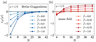
Figure B1: Relative error of the approximate free energy density for $\tilde{\mu}=\tilde{h}=0$ obtained by the (a) Bethe-Guggenheim and (b) mean field approximation as a function of the system size. Up to $N=36$ each point corresponds to the relative error for a square lattice of size $\sqrt{N}\times\sqrt{N}$ with free boundary conditions and $\varphi=1/2$ closed bonds. For $N=42$ a rectangular lattice of size $6\times 7$ with free boundary conditions is considered.

In Fig. B1 we compare the accuracy of the Bethe-Guggenheim (a) and mean field (b) approximations by means of the relative error $\epsilon^{\rm BG,MF}_{N}\left(\varphi\right)\equiv 1-\tilde{f}_{N}^{\rm BG/MF}\left(\varphi\right)/\tilde{f}_{N}\left(\varphi\right)$ between the exact and approximate free energy density for a two-dimensional lattice with $\varphi=1/2$ closed bonds as a function of the system size $N$. We find that the Bethe-Guggenheim approximation converges to the exact free energy density with increasing $N$, regardless of the coupling strength $\tilde{J}$. Conversely, the mean field approximation diverges with both, increasing system size $N$ and coupling strength $\tilde{J}$.

B.2 Phase diagram

B.2.1 Independence of the binodal and spinodal line on $\tilde{\mu}$

Let us write $\tilde{\rm f}\left(\varphi\right)=\tilde{\mu}\varphi+\tilde{\rm g}\left(\varphi\right)$, where $\tilde{\rm g}\left(\varphi\right)$ is the remainder of the free energy density after leaving out all linear terms in $\varphi$. Plugging this expression into the binodal line equations given by Eq. (14) gives

$$\tilde{\mu}+\tilde{\rm g}^{\prime}\left(\varphi_{l}\right) = \tilde{\mu}+\tilde{\rm g}^{\prime}\left(\varphi_{g}\right),$$

$$\tilde{\mu}+\frac{\tilde{\rm g}\left(\varphi_{l}\right)-\tilde{\rm g}\left(\varphi_{g}\right)}{\varphi_{l}-\varphi_{g}} = \tilde{\mu}+\tilde{\rm g}^{\prime}\left(\varphi_{l}\right).$$ (B10)

Clearly $\tilde{\mu}$ cancels and therefore does not affect the binodal line.

The spinodal line – also known as the stability boundary – denotes the boundary between the metastable and unstable state, and is given by $\tilde{\rm f}^{\prime\prime}(\varphi)=0$. The spinodal line is as well not affected by $\tilde{\mu}$, since the second derivative of the linear term vanishes.

B.2.2 Binodal line for zero force

At zero force the binodal line equations simplify to $\tilde{\rm f}^{\prime}(\varphi)|^{\tilde{h}=0}_{\tilde{\mu}=0}=0$. Our aim is to solve this equation for $\Omega_{\varphi}$ (defined as Eq. (9) in the thermodynamic limit) in Eq. (12), and then use the inverse relation

$$\tilde{J}\left(\varphi,\Omega_{\varphi}\right)=\frac{1}{4}\ln{\left(\frac{\left(\varphi-\Omega_{\varphi}\right)\left(1-\varphi-\Omega_{\varphi}\right)}{\Omega_{\varphi}^{2}}\right)},$$ (B11)

to obtain the binodal line. Notice that it follows from Eq. (9) that $\Omega_{\varphi}\geq 0$ for $0\leq\varphi\leq 1$, and this constraint has to be obeyed by the implicit solution for $\Omega_{\varphi}$. Evaluating the total derivative with respect to $\varphi$ of Eq. (12) gives

$$\tilde{\rm f}^{\prime}(\varphi,\Omega_{\varphi})|_{\tilde{J},\tilde{\mu}=0}{=}\partial_{\varphi}\tilde{\rm f}(\varphi,\Omega_{\varphi})|_{\tilde{J},\tilde{\mu}=0}+\partial_{\Omega_{\varphi}}\tilde{\rm f}(\varphi,\Omega_{\varphi})|_{\tilde{J},\tilde{\mu}=0}\cdot\Omega^{\prime}_{\varphi},$$ (B12)

where $\Omega^{\prime}_{\varphi}=\partial_{\varphi}\Omega_{\varphi}|_{\tilde{J}}$. Since $\Omega_{\varphi}$ was obtained by solving $\partial_{\Omega_{\varphi}}\tilde{\rm f}(\varphi,\Omega_{\varphi})|_{\tilde{J},\tilde{\mu}=0}=0$ the second term in Eq. (B12) vanishes while the first term yields

$$\frac{2\tilde{h}}{\left(1+\varphi\right)^{2}}+\left(1-\bar{z}\right)\ln{\left(\frac{\varphi}{1-\varphi}\right)}+\frac{\bar{z}}{2}\ln{\left(\frac{\varphi-\Omega_{\varphi}}{1-\varphi-\Omega_{\varphi}}\right)}.$$ (B13)

Setting $\tilde{h}=0$ in Eq. (B13), and introducing $\chi_{\varphi}\equiv\varphi/(1-\varphi)$ and $\alpha\equiv(\bar{z}-1)/\bar{z}$ we find the following solution for $\Omega_{\varphi}$ evaluated on the zero-force binodal line

$$\Omega_{\varphi}(\tilde{J}_{\rm b}(\varphi)|^{\tilde{h}=0}_{\tilde{\mu}=0})=\frac{\chi_{\varphi}}{1+\chi_{\varphi}}\frac{1-\chi_{\varphi}^{2\alpha-1}}{1-\chi_{\varphi}^{2\alpha}}.$$ (B14)

Plugging Eq. (B14) into Eq. (B11) yields Eq. (15) for the zero-force binodal line, which was also reported in [116, 79, 139]. For $\tilde{h}\neq 0$ the binodal line can be obtained by solving Eq. (14) numerically.

B.2.3 Spinodal line

To determine the spinodal line we calculate the second derivative of the Bethe-Guggenheim free energy density

$$\tilde{\rm f}^{\prime\prime}(\varphi,\Omega_{\varphi})=-\frac{4\tilde{h}}{\left(1+\varphi\right)^{3}}+\frac{1-\bar{z}}{\varphi\left(1-\varphi\right)}+\frac{\bar{z}}{2}\frac{\left(1-2\Omega_{\varphi}\right)+2\left(2\varphi-1\right)\Omega_{\varphi}^{\prime}}{\left(\varphi-\Omega_{\varphi}\right)\left(1-\varphi-\Omega_{\varphi}\right)}+\frac{\bar{z}}{2}\frac{\left[2\varphi\left(1-\varphi\right)-\Omega_{\varphi}\right]\Omega_{\varphi}^{\prime 2}}{\Omega_{\varphi}\left(\varphi-\Omega_{\varphi}\right)\left(1-\varphi-\Omega_{\varphi}\right)}.$$ (B15)

Eq. (B15) contains $\Omega^{\prime}_{\varphi}$, which we want to express in terms of $\Omega_{\varphi}$. Therefore we use Eq. (B11) and differentiate both sides with respect to $\varphi$ for fixed $\tilde{J}$, yielding

$$\Omega_{\varphi}^{\prime}=\frac{\Omega_{\varphi}\left(1-2\varphi\right)}{2\varphi\left(1-\varphi\right)-\Omega_{\varphi}}.$$ (B16)

Plugging Eq. (B16) into Eq. (B15) gives

$$\tilde{\rm f}^{\prime\prime}(\varphi,\Omega_{\varphi})=-\frac{4\tilde{h}}{\left(1+\varphi\right)^{3}}+\frac{1-\bar{z}}{\varphi\left(1-\varphi\right)}+\frac{\bar{z}}{2\varphi\left(1-\varphi\right)-\Omega_{\varphi}}=0.$$ (B17)

Solving Eq. (B17) for $\Omega_{\varphi}$ yields $\Phi(\varphi,\tilde{h})$ in Eq. (16), which must be non-negative thus implying that Eq. (16) is valid for $(2-\bar{z})/8\tilde{h}\leq\varphi(1-\varphi)/(1+\varphi)^{3}\leq(1-\bar{z})/4\tilde{h}$.

B.2.4 Statical critical point

We derive the Bethe-Guggenheim statical critical point in the form of a convergent Newton series [80, 82, 142]. We determine the statical critical point from

$$\tilde{\rm f}^{\prime\prime\prime}(\varphi,\Omega_{\varphi})=\frac{12\tilde{h}}{\left(1+\varphi\right)^{4}}+\frac{\left(1-\bar{z}\right)\left(2\varphi-1\right)}{\varphi^{2}\left(1-\varphi\right)^{2}}-\frac{\bar{z}\left[2\left(1-2\varphi\right)-\Omega_{\varphi}^{\prime}\right]}{\left(2\varphi\left(1-\varphi\right)-\Omega_{\varphi}\right)^{2}}=0.$$ (B18)

Using Eq. (B16) for $\Omega_{\varphi}^{\prime}$ we get

$$\frac{12\tilde{h}}{\left(1+\varphi\right)^{4}}+\frac{\left(1-\bar{z}\right)\left(2\varphi-1\right)}{\varphi^{2}\left(1-\varphi\right)^{2}}+\frac{\bar{z}\left(2\varphi-1\right)\left[4\varphi\left(1-\varphi\right)-3\Omega_{\varphi}\right]}{\left(2\varphi\left(1-\varphi\right)-\Omega_{\varphi}\right)^{3}}=0.$$ (B19)

To simplify Eq. (B19) further we introduce the auxiliary parameter $\alpha_{\tilde{h}}\equiv 12\tilde{h}$ and use the fact that the critical point lies on the spinodal line, which allows us to use Eq. (17) for $\Omega_{\varphi}$ and leads to

$$g\left(\varphi\right)\equiv\alpha_{\tilde{h}}\varphi^{2}\left(1-\varphi\right)^{2}+\left(1+\varphi\right)^{4}\left(2\varphi-1\right)\gamma_{\bar{z}}\left(\varphi\right)=0,$$ (B20)

with

$$\gamma_{\bar{z}}\left(\varphi\right)\equiv 1-\frac{1}{\bar{z}}\left(3-\frac{2}{\bar{z}}\right)+\frac{2\alpha_{\tilde{h}}}{\bar{z}}\left(1-\frac{1}{\bar{z}}\right)\Lambda\left(\varphi\right)-\frac{\alpha_{\tilde{h}}^{2}}{3\bar{z}}\left(1-\frac{2}{\bar{z}}\right)\Lambda^{2}\left(\varphi\right)-\frac{2\alpha_{\tilde{h}}^{3}}{27\bar{z}^{2}}\Lambda^{3}\left(\varphi\right),$$ (B21)

and $\Lambda\left(\varphi\right)\equiv\varphi(1-\varphi)/(1+\varphi)^{3}$. For $\tilde{h}=0$ the solution of Eq. (B20) is given by $\varphi^{\rm s}_{\rm crit,BG}=1/2$, and the corresponding statical critical point is given by $\tilde{J}^{\rm s}_{\rm crit,BG}=\ln{\left(\bar{z}/(\bar{z}-2)\right)}/\bar{2}$.

For non-zero force we solve Eq. (B20) by means of a “quadratic” Newton series as explained in more detail in Appendix D. The main result for the statical critical fraction obtained by the quadratic Newton series reads

$$\!\!\!\!\!\!\!\!\!\varphi^{\rm s}_{\rm crit,BG} \approx \frac{1}{2}-\frac{g^{\prime}\left(\frac{1}{2}\right)}{g^{\prime\prime}\left(\frac{1}{2}\right)}+\left[\frac{g^{\prime}\left(\frac{1}{2}\right)^{2}}{g^{\prime\prime}\left(\frac{1}{2}\right)^{2}}-2\frac{g\left(\frac{1}{2}\right)}{g^{\prime\prime}\left(\frac{1}{2}\right)}\right]^{1/2}$$ (B22)

$$= \frac{1}{2}-\frac{3}{2^{4}}\frac{\delta_{\bar{z}}(\tilde{h})}{\nu_{\bar{z}}(\tilde{h})}+\frac{3}{2^{4}}\left[\frac{\delta^{2}_{\bar{z}}(\tilde{h})}{\nu^{2}_{\bar{z}}(\tilde{h})}-\frac{2^{6}}{3^{4}}\frac{\bar{z}^{2}\tilde{h}}{\nu_{\bar{z}(\tilde{h})}}\right]^{1/2},$$

where $g^{\prime}\left(\varphi\right)=\partial_{\varphi}g(\varphi)$, $g^{\prime\prime}\left(\varphi\right)=\partial^{2}_{\varphi}g(\varphi)$, and the auxiliary functions $\delta_{\bar{z}}(\tilde{h})$ and $\nu_{\bar{z}}(\tilde{h})$ are defined as

$$\delta_{\bar{z}}(\tilde{h})\equiv(\bar{z}-1-\frac{2^{6}}{3^{5}}\tilde{h}^{2})(\bar{z}-2+\frac{2^{4}}{3^{2}}\tilde{h})+\frac{2^{13}}{3^{9}}\tilde{h}^{3},$$ (B23)

and

$$\nu_{\bar{z}}(\tilde{h})\equiv(\bar{z}-1+\frac{2^{5}}{3^{5}}\tilde{h}^{2})(\bar{z}-2+\frac{2^{2}}{3^{2}}\tilde{h})-\frac{2}{3^{2}}\bar{z}^{2}\tilde{h}+\frac{2^{7}}{3^{9}}\tilde{h}^{3},$$ (B24)

respectively.

The statical critical coupling $\tilde{J}^{\rm s}_{\rm crit}$ is obtained by inserting Eq. (B22) into Eq. (16), and the result is depicted by the gradient line Fig. 5 in the main text, where the black symbols represent the fully converged Newton’s series (D17), as well as in Fig. C1 where the gradient line depicts the fully converged Newton’s series.

Appendix C Mean field approximation

C.1 Partition function

Within the mean field approximation the partition function reads

$$Z_{k}^{\rm MF}=\binom{N}{k}\mathrm{e}^{\tilde{J}\bar{z}(N/2-2X^{*}_{k})},$$ (C1)

with $X^{*}_{k}\equiv k\left(N-k\right)/N$, such that the corresponding free energy density in the thermodynamic limit attains the form

$$\tilde{\rm f}^{\rm MF}(\varphi)=-\tilde{\mu}\varphi+\frac{2\tilde{h}\varphi}{1+\varphi}+\frac{1}{2}\tilde{J}\bar{z}[4\varphi(1-\varphi)-1]+\Xi_{\Delta}(\varphi),$$ (C2)

where $\Xi_{\Delta}(x)\equiv\Xi(x)+\Xi(1-x)$.

C.2 Phase diagram

We now evaluate the binodal and spinodal line, as well as the statical critical point within the mean field approximation. The corresponding exact solutions for the Bethe-Guggenheim approximation are given by Eqs. (15)-(19).

C.2.1 Binodal line for zero force

In the absence of an external field, $\tilde{h}=0$, the binodal line is given by

$$\tilde{J}_{\rm b,MF}(\varphi)|_{\tilde{h}=0}=\frac{1}{2\bar{z}(2\varphi-1)}\ln{\left(\frac{\varphi}{1-\varphi}\right)}.$$ (C3)

This solution is well known and has been reported in the literature extensively [143, 116, 79, 139]. For $\tilde{h}\neq 0$ we solve for the binodal line numerically.

C.2.2 Spinodal line

The spinodal line is in turn given by the solution of $\tilde{\rm f}^{{\rm MF}^{\prime\prime}}(\varphi)=0$ and reads

$$\tilde{J}_{\rm s,MF}(\varphi)=\frac{1}{4\bar{z}}\left(\frac{1}{\varphi\left(1-\varphi\right)}-\frac{4\tilde{h}}{\left(1+\varphi\right)^{3}}\right).$$ (C4)

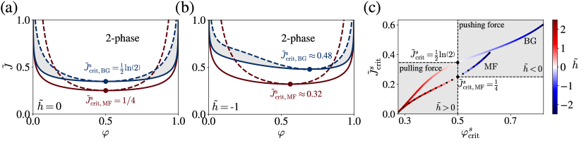
Figure C1: Comparison of the Bethe-Guggenheim (BG) and mean field (MF) binodal line, spinodal line, and statical critical point. (a-b) Phase diagram for (a) zero force and (b) pushing force $\tilde{h}=-1$; the full and dashes lines depict the binodal and spinodal line, respectively. Red lines correspond to the mean field approximation obtained with Eqs. (C3) (for zero force) and (C4). Blue lines correspond to the Bethe-Guggenheim approximation in Eqs. (15) (for zero force) and (16). The shaded area depicts the region where the system is metastable for the Bethe-Guggenheim approximation. The blue and red circle depict the statical critical point $(\varphi^{\rm s}_{\rm crit},\tilde{J}^{\rm s}_{\rm crit})$ for the mean field and Bethe-Guggenheim approximation, respectively. (c) The statical critical point as a function of the force $\tilde{h}$. For the Bethe-Guggenheim approximation is the result obtained with a converged Newton’s series (see Eq. (D17)), whereas the mean field result is obtained by considering the first ten terms of Eq. (C13).

C.2.3 Statical critical point

The statical critical point is given by the solution of $\tilde{\rm f}^{\prime\prime\prime{\rm MF}}(\varphi)=0$, which after introducing the parameter $\alpha_{\tilde{h}}\equiv 12\tilde{h}$ translates into solving the algebraic equation

$$\alpha_{\tilde{h}}\varphi^{2}\left(1-\varphi\right)^{2}+\left(1+\varphi\right)^{4}\left(2\varphi-1\right)=0.$$ (C5)

Notice that $\bar{z}$, the average coordination number, does not enter Eq. (C5). When $\tilde{h}=0$ the solution is $\varphi^{\rm s}_{\rm crit,MF}=1/2$, and the corresponding statical critical point is given by $\tilde{J}^{\rm s}_{\rm crit,MF}=\bar{z}^{-1}$. To solve Eq. (C5) for non-zero force we first note that $0\leq\varphi^{\rm s}_{\rm crit,MF}\leq 1$, and therefore we can divide Eq. (C5) by $\left(1+\varphi\right)^{4}$. Upon introducing the variable $w=2\varphi-1$ we get the equation

$$\frac{w}{f\left(w\right)}=-\alpha_{\tilde{h}},$$ (C6)

with $f\left(w\right)=\left(w+1\right)^{2}\left(w-1\right)^{2}\left(w+3\right)^{-4}$. Now we recall the Lagrange inversion theorem: Let $f(w)$ be analytic in some neighborhood of the point $w=0$ (of the complex plane) with $f(0)\neq 0$ and let it satisfy the equation

$$\frac{w}{f(w)}=\alpha.$$ (C7)

Then $\exists a,b\in\mathbbm{R}^{+}$ such that for $|\alpha|<a$ Eq. (C7) has only a single solution in the domain $|w|<b$. According to the Lagrange-Bürmann formula this unique solution is an analytical function of $\alpha$ given by

$$w=\sum_{k=1}^{\infty}\frac{\alpha^{k}}{k!}\left[\frac{d^{k-1}}{dw^{k-1}}f(w)^{k}\right]_{w=0}.$$ (C8)

Notice that Eq. (C6) has the form of Eq. (C7), and therefore we can use Eq. (C8) to obtain $\varphi^{\rm s}_{\rm crit,MF}$. To evaluate the derivative inside Eq. (C8) it is convenient to write $f(w)^{k}=g(w)h(w)$, with $g(w)\equiv(w+1)^{2k}(w-1)^{2k}=(w^{2}-1)^{2k}$ and $h(w)\equiv(w+3)^{-4k}$. Using the fact that

$$\frac{d^{n}}{dw^{n}}g(w)h(w)|_{w=0}=\sum_{k=0}^{n}\binom{n}{k}g^{(n-k)}(0)h^{(k)}(0),$$ (C9)

as well as

$$\frac{d^{n}}{dw^{n}}(w^{2}-1)^{2k}|_{w=0}=\cos{\left(\frac{\pi n}{2}\right)}n!\binom{2k}{n/2}$$ (C10)

and

$$\frac{d^{n}}{dw^{n}}\left(w+3\right)^{-4k}|_{w=0}=(-1)^{n}3^{-4k-n}\frac{(4k+n-1)!}{(4k-1)!},$$ (C11)

we find

$$\frac{d^{k-1}}{dw^{k-1}}f(w)^{k} |_{w=0}=\frac{\left(-1\right)^{k-1}3^{-5k+1}\left(k-1\right)!\left(2k\right)!}{\left(4k-1\right)!}$$

$$\times \sum_{m=0}^{\lfloor\frac{k-1}{2}\rfloor}\frac{\left(-9\right)^{m}\left(5k-2(1+m)\right)!}{m!\left(2k-m\right)!\left(k-1-2m\right)!}.$$ (C12)

Plugging Eq. (C12) into Eq. (C8) and using the relation $\varphi=(1+w)/2$ we find $\varphi^{s}_{\rm crit,MF}=\varphi^{s,0}_{\rm crit,MF}-6\sum_{k=1}^{\infty}\delta\varphi_{k}(\tilde{h})$ with

$$\delta\varphi_{k}(\tilde{h})=(4\tilde{h})^{k}\frac{\left(2k\right)!}{\left(4k\right)!}\sum\limits_{m=0}^{\lfloor\frac{k-1}{2}\rfloor}\frac{\left(-9\right)^{m-2k}\left(5k-2(1+m)\right)!}{m!\left(2k-m\right)!\left(k-1-2m\right)!}.$$ (C13)

The statical critical coupling for non-zero force, $\tilde{J}^{\rm s}_{\rm crit,MF}(\tilde{h})$, is obtained by plugging $\varphi^{s}_{\rm crit,MF}$ into Eq. (C4).

In Fig. C1 we plot the statical critical point for the Bethe-Guggenheim and mean field approximation as a function of the force $\tilde{h}$. For large pulling force ($\tilde{h}\geq 2$) the statical critical point is pushed towards lower values of $\tilde{J}$, and as a consequence the Bethe-Guggenheim and mean field solution start to coincide. For other values of $\tilde{h}$, however, the Bethe-Guggenheim and mean field solutions disagree strongly, in particular for weak forces $|\tilde{h}|\to 0$.

To compare the critical points for weak pulling/pushing forces in more detail we inspect the perturbation series given in Eqs. (18) and (19) and compare it with the first two terms of Eq. (C13). Defining $\tilde{J}^{s}_{\rm crit,MF}=\tilde{J}^{s,0}_{\rm crit,MF}-\delta\tilde{J}^{s}_{\rm crit,MF}(\tilde{h})+\mathcal{O}(\tilde{h}^{3})$ and $\varphi^{s}_{\rm crit,MF}=\varphi^{s,0}_{\rm crit,MF}-\delta\varphi_{\rm crit,MF}(\tilde{h})+\mathcal{O}(\tilde{h}^{3})$, we get

$$\delta\tilde{J}^{\rm s}_{\rm crit,MF}(\tilde{h})=\frac{8}{27}\frac{1}{\tilde{z}}\left(\tilde{h}+\frac{2}{27}\tilde{h}^{2}\right),$$ (C14)

and

$$\delta\varphi^{\rm s}_{\rm crit,MF}(\tilde{h})=\frac{2}{27}\left(\tilde{h}+\frac{16}{81}\tilde{h}^{2}\right).$$ (C15)

Interestingly, whereas the Bethe-Guggenheim critical point depends on $\bar{z}$ (see Eq. (19)), the mean field result in Eq. (C15) does not. In the limit $\bar{z}\rightarrow\infty$ we find that the Bethe-Guggenheim statical critical point converges to the mean field solution, which is to be expected.

Appendix D Equation of state in the thermodynamic limit

Here we derive the equation of state in the thermodynamic limit using the saddle-point technique, i.e.

$$\langle\varphi\rangle_{\rm TD}\equiv\lim_{N\to\infty}\frac{\displaystyle{\int_{0}^{1}\varphi\mathrm{e}^{-N\tilde{\rm f}(\varphi)}d\varphi}}{\displaystyle{\int_{0}^{1}\mathrm{e}^{-N\tilde{\rm f}(\varphi)}d\varphi}}\simeq\\ \lim_{N\to\infty}\frac{\displaystyle{\int_{0}^{1}\sum\limits_{i=1}^{M}\varphi^{0}_{i}\mathrm{e}^{-N\tilde{\rm f}^{\prime\prime}(\varphi^{0}_{i})(\varphi-\varphi^{0}_{i})^{2}}d\varphi}}{\displaystyle{\int_{0}^{1}\sum\limits_{i=1}^{M}\mathrm{e}^{-N\tilde{\rm f}^{\prime\prime}(\varphi^{0}_{i})(\varphi-\varphi^{0}_{i})^{2}}d\varphi}}=\sum\limits_{i=1}^{M}c_{i}\varphi^{0}_{i},$$ (D1)

with

$$c_{j} = \lim_{N\to\infty}\frac{\displaystyle{\int_{0}^{1}\mathrm{e}^{-N\tilde{\rm f}^{\prime\prime}(\varphi^{0}_{j})(\varphi-\varphi^{0}_{j})^{2}}d\varphi}}{\displaystyle{\int_{0}^{1}\sum\limits_{i=1}^{M}\mathrm{e}^{-N\tilde{\rm f}^{\prime\prime}(\varphi^{0}_{i})(\varphi-\varphi^{0}_{i})^{2}}d\varphi}}$$ (D2)

$$\simeq \left(1+\sum_{i=1|i\neq j}^{M}\sqrt{\tilde{\rm f}^{\prime\prime}(\varphi^{0}_{j})/\tilde{\rm f}^{\prime\prime}(\varphi^{0}_{i})}\right)^{-1},$$

and $\varphi^{0}_{1},\varphi^{0}_{2},...,\varphi^{0}_{M}$ denote the locations of the local minima of the Bethe-Guggenheim free energy density ${\rm\tilde{f}}(\varphi)\equiv{\rm\tilde{f}^{BG}}(\varphi)$ in Eq. (12). The idea behind Eq. (D1) is that in the large $N$ limit we expect the integral over $\varphi$ to be dominated by the immediate neighborhood of the local minima of $\tilde{\rm f}\left(\varphi\right)$. We may therefore approximate the exponent by its Taylor expansion around these extremal points. In general special care has to be taken when one of the global minima lies at the boundary of the integration interval [144], which turns out not to be the case here.

The locations of the local minima, maxima, and saddle points of the Bethe-Guggenheim free energy density are given by the solution of $\tilde{\rm f}^{\prime{\rm BG}}(\varphi)=0$. Notice that here we do not set the intrinsic binding-affinity $\tilde{\mu}$ to zero, since we are interested in the stationary points and not the binodal line. We solve the former equation for $\Omega_{\varphi}$ and substitute the solution into Eq. (B11) which gives

$$\tilde{J}=\frac{1}{2}\ln{\left(\frac{1-\chi_{\varphi}}{c_{\tilde{\mu},\tilde{h}}^{-1}(\chi_{\varphi})\chi_{\varphi}^{1-\alpha}-c_{\tilde{\mu},\tilde{h}}(\chi_{\varphi})\chi_{\varphi}^{\alpha}}\right)},$$ (D3)

where $\chi_{\varphi}\equiv\varphi/(1-\varphi)$, $\alpha\equiv(\bar{z}-1)/\bar{z}$, and

$$c_{\tilde{\mu},\tilde{h}}(\chi_{\varphi})\equiv\mathrm{e}^{\frac{\tilde{\mu}}{\bar{z}}}\mathrm{e}^{-\frac{2}{\bar{z}}\left(\frac{1+\chi_{\varphi}}{1+2\chi_{\varphi}}\right)^{2}\tilde{h}}.$$ (D4)

Rewriting Eq. (D3) gives

$$\chi_{\varphi}-\mathrm{e}^{2\tilde{J}}\left(c_{\tilde{\mu},\tilde{h}}(\chi_{\varphi})\chi^{\alpha}_{\varphi}-c^{-1}_{\tilde{\mu},\tilde{h}}(\chi_{\varphi})\chi_{\varphi}^{1-\alpha}\right)-1=0.$$ (D5)

For a two-dimensional square lattice in the thermodynamic limit we have $\bar{z}=4$ and so $\alpha=3/4$. Upon introducing the auxiliary variable $\xi\equiv\chi_{\varphi}^{1/4}$ we obtain the transcendental equation

$$g(\xi)\equiv\xi^{4}-\mathrm{e}^{2\tilde{J}}\left(c_{\tilde{\mu},\tilde{h}}(\xi)\xi-c_{\tilde{\mu},\tilde{h}}^{-1}(\xi)\xi^{-1}\right)\xi^{2}-1=0.$$ (D6)

To solve for the roots of $g(\xi)$ we first consider the force-free scenario $\tilde{h}=0$ and afterwards solve for the general case.

D.1 Zero force

For zero force $g(\xi)$ reduces to a quartic in $\xi$. The roots of a general quartic equation are known and are given by

$$\xi_{1,2}=\frac{\mathcal{Y}_{+}}{4}-S\pm\frac{1}{2}\sqrt{\frac{3}{4}\mathcal{Y}_{+}^{2}+\frac{\mathcal{Y}_{-}-\frac{1}{8}\mathcal{Y}_{+}^{3}}{S}-4S^{2}},$$ (D7a)

$$\xi_{3,4}=\frac{\mathcal{Y}_{+}}{4}+S\pm\frac{1}{2}\sqrt{\frac{3}{4}\mathcal{Y}_{+}^{2}-\frac{\mathcal{Y}_{-}-\frac{1}{8}\mathcal{Y}_{+}^{3}}{S}-4S^{2}},$$ (D7b)

where $\mathcal{Y}_{\pm}=\mathrm{e}^{2\tilde{J}\pm\tilde{\mu}/4}$ and

$$S=\frac{1}{2}\sqrt{\frac{1}{4}\mathcal{Y}_{+}^{2}+\frac{1}{3}\left(W+\frac{\Delta_{0}}{W}\right)},$$ (D8)

$$W=\left(\frac{\Delta_{1}+\sqrt{\Delta_{1}^{2}-4\Delta_{0}^{3}}}{2}\right)^{1/3},$$ (D9)

$$\Delta_{0}=3\mathrm{e}^{4\tilde{J}}-12,\,\,\,\Delta_{1}=-54\mathrm{e}^{4\tilde{J}}\Delta_{\tilde{\mu}},\,\,\,\Delta_{\tilde{\mu}}=\sinh(\tilde{\mu}/2).$$ (D10)

Fig. D1 depicts the four solutions in Eqs. (D7a) and (D7b) as a function of $\tilde{J}$ for various values of $\tilde{\mu}$.

To determine the local minima we must analyze the properties of these roots starting with the sign of the discriminant, given by

$$\Delta=\frac{1}{27}\left(4\Delta_{0}^{3}-\Delta_{1}^{2}\right)=4\left(\mathrm{e}^{4\tilde{J}}-4\right)^{3}-108\mathrm{e}^{8\tilde{J}}\Delta_{\tilde{\mu}}^{2}.$$ (D11)

For $\Delta<0$ there are two distinct real roots and two complex conjugate roots, whereas for $\Delta>0$ there are either four real roots or four imaginary roots, where the former scenario applies here. The discriminant is zero at the critical coupling value

$$\tilde{J}_{\Delta=0}=\frac{1}{4}\ln{\left(\frac{3\Delta_{\tilde{\mu}}^{2}\left(9\Delta_{\tilde{\mu}}^{2}+8\right)}{\Phi^{1/3}}+3\Phi^{1/3}+9\Delta_{\tilde{\mu}}^{2}+4\right)},$$ (D12)

with

$$\Phi=27\Delta_{\tilde{\mu}}^{6}+36\Delta_{\tilde{\mu}}^{4}+8\Delta_{\tilde{\mu}}^{2}[1+(1+\Delta_{\tilde{\mu}}^{2})^{1/2}].$$ (D13)

Increasing the coupling strength above $\tilde{J}_{\Delta=0}$ gives rise to a local maximum in the free energy landscape, its position being $\xi^{4}_{4}/(1+\xi^{4}_{4})$ (see purple line in Fig. D1).

D.1.1 Zero intrinsic binding-affinity

For zero intrinsic binding-affinity we note that $\tilde{J}_{\Delta=0}$ coincides with the statical critical point $\tilde{J}^{s}_{\rm crit}=\ln{(2)}/2$. In this limit the four solutions  (D7a) and (D7b) simplify substantially, and the corresponding locations of the local minima – which are also global minima – are given by (see Fig. D1a)

$$\varphi^{0}_{\rm 1,2}|_{\tilde{\mu}=0}^{\tilde{h}=0}=\begin{dcases*}\frac{1}{2}&, $0\leq\tilde{J}\leq\tilde{J}^{s}_{\rm crit}$\\ \frac{1}{2}\left[1\pm\frac{\mathrm{e}^{2\tilde{J}}\sqrt{\mathrm{e}^{4\tilde{J}}-4}}{(\mathrm{e}^{4\tilde{J}}-2)}\right]&, $\tilde{J}\geq\tilde{J}^{s}_{\rm crit}$\end{dcases*}.$$ (D14)

For $\tilde{J}\leq\tilde{J}^{s}_{\rm crit}$ there is a single global minimum in the free energy landscape, and therefore the weight $c_{1}$ given by Eq. (D2) becomes unity. For $\tilde{J}>\tilde{J}^{s}_{\rm crit}$ the global minima are two-fold degenerate and located equidistantly from the local maximum at $\varphi=1/2$. Since both global minima have the same curvature, we find that the weights are given by $c_{1,2}=1/2$. Combining these results we obtain the average fraction of closed bonds in the thermodynamic limit for zero intrinsic binding-affinity in the form

$$\langle\varphi\rangle_{\rm TD}|_{\tilde{\mu}=0}^{\tilde{h}=0}=\frac{1}{2},$$ (D15)

which was to be expected since the coupling $\tilde{J}$ does not favor bonds to be open nor closed.

D.1.2 Non-zero intrinsic bining-affinity

For non-zero intrinsic binding-affinity, $\tilde{\mu}\neq 0$, the free energy landscape is tilted, resulting in a unique global minimum with corresponding weight $c_{1}=1$. As a result, the average fraction of closed bonds, which is dominated by this minimum $\varphi^{0}_{1}$, is given by (see Fig. D1(b) and (c))

$$\langle\varphi\rangle_{\rm TD}|_{\tilde{\mu}\neq 0}^{\tilde{h}=0}\begin{dcases*}\frac{\xi_{1}^{4}}{1+\xi_{1}^{4}}&, $0\leq\tilde{J}\leq\ln{\min{\{\sqrt{2},s_{0}\}}}$\\ \frac{\xi_{3}^{4}}{1+\xi_{3}^{4}}&, $\tilde{J}\geq\ln{\min{\{\sqrt{2},s_{0}\}}}$,\end{dcases*}.$$ (D16)

where $\ln{s_{0}}\equiv\ln{\sqrt{2\sqrt{2}}\mathrm{e}^{-\tilde{\mu}/4}}$ denotes the coupling strength that solves for the root of $S$ in Eq. (D8).

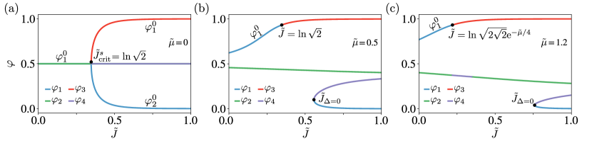
Figure D1: Stationary points of the Bethe-Guggenheim free energy density for zero force, given by Eqs. (D7a) and (D7b), as a function of the coupling strength $\tilde{J}$. From left to right we consider increasing values of the intrinsic binding-affinity $\tilde{\mu}$. The variable $\varphi^{0}_{1,2}$ indicates the location of the global minima, which is given by Eq. (D14) for zero intrinsic binding-affinity (a), and given by Eq. (D16) for non-zero intrinsic binding-affinity (b and c). The coupling value $\tilde{J}_{\Delta=0}$, given by Eq. (D12), indicates the coupling strength where all four solutions become real, and denotes the first appearance of a local maximum given by $\varphi_{4}$.

D.2 Non-Zero force

We determine the roots of $g(\xi)$ for a non-zero force by means of a convergent Newton series yielding the exact result [80, 82, 142]

$$\xi=\xi_{0}-\sum\limits_{k=1}^{\infty}\frac{\left[g^{\left(0\right)}\left(\xi_{0}\right)\right]^{k}}{\left[g^{\left(1\right)}\left(\xi_{0}\right)\right]^{2k-1}}\frac{\det{\mathcal{A}_{k}\left(\xi_{0}\right)}}{\left(k-1\right)!},$$ (D17)

where $\xi_{0}$ is an initial guess in a convex neighborhood around $\xi$, $g^{\left(i\right)}\left(\xi_{0}\right)$ denotes the $i$th derivative of $g(\xi)$ at the point $\xi_{0}$, and $\mathcal{A}_{k}\left(\xi_{0}\right)$ are almost triangular matrices of size $\left(k-1\right)\times\left(k-1\right)$ with elements

$$\mathcal{A}^{ij}_{k}\left(\xi_{0}\right)=\frac{g^{\left(i-j+2\right)}\left(\xi_{0}\right)\theta\left(i-j+1\right)}{\left(i-j+2\right)!}\times$$

$$\left(k\left[i-j+1\right]\theta\left(j-2\right)+i\theta\left(1-j\right)+j-1\right),$$ (D18)

where $\theta\left(x\right)$ denotes the Heaviside step function, i.e. $\theta\left(x\right)=1$ if $x\geq 0$ and 0 otherwise, and we symbolically set $\det\mathcal{A}_{1}=1$. The determinant of almost triangular matrices, also known as upper/lower Hessenberg matrices, can be efficiently calculated using a recursion formula [145], for which a numerical implementation can be found in [146]. If we set $g^{\left(3\right)}=g^{\left(4\right)}=...=0$ in the almost triangular matrices, the resulting matrix $\mathcal{\tilde{A}}_{k}$ becomes triangular, implying that its determinant is simply given by the product of its diagonal elements. Making the substitution $\mathcal{A}_{k}\rightarrow\mathcal{\tilde{A}}_{k}$ in Eq. (D17) yields the so-called “quadratic approximation” [82, 142]

$$\xi\approx\xi_{0}-\frac{g^{\left(1\right)}\left(\xi_{0}\right)-\sqrt{g^{\left(1\right)}\left(\xi_{0}\right)^{2}-2g^{\left(0\right)}\left(\xi_{0}\right)g^{\left(2\right)}\left(\xi_{0}\right)}}{g^{\left(2\right)}\left(\xi_{0}\right)}.$$ (D19)

that becomes exceedingly accurate when the root moves close to $\xi_{0}$. For the initial point $\xi_{0}$ we use the ansatz

$$\xi_{0}=\exp\left(\frac{\tilde{\mu}}{4}-\frac{2}{9}\tilde{h}+{\rm sign}\left[\frac{\tilde{\mu}}{4}-\frac{2}{9}\tilde{h}\right]\frac{6}{5}\tilde{J}\right),$$ (D20)

which is derived by considering an adapted form of Eqs. (D7a) and (D7b) in combination with the implementation of the force term. The weight $2/9$ is derived from the term $(1+\xi^{4})^{2}/2(1+2\xi^{4})^{2}$ in Eq. (D4) evaluated at the point $\xi=1$ (corresponding to $\varphi=1/2$), and the weight $6/5$ in front of $\tilde{J}$ was selected empirically. This choice assures that Eq. (D6) satisfies the Lipschitz condition between $\xi_{0}$ and the root $\xi$ and thus assures the convergence of the Newton’s series.

Plugging Eq. (D20) into Eq. (D19), and using the relation $\varphi^{0}_{1}=\xi^{4}/(1+\xi^{4})$, we obtain the location of the global minimum - and thus $\langle\varphi\rangle_{\rm TD}$ - for non-zero force. Notably, the ansatz given by Eq. (D20) also provides a numerically correct solution for a zero force and non-zero intrinsic binding-affinity. For completeness we write down explicitly all the terms which are used to evaluate Eq. (D19) (higher order terms entering the fully converged series in Eq. (D17) are omitted as they are lengthy).

Let $g\left(\xi\right)$ be given by Eq. (D6). Introducing the auxiliary functions

$$\alpha_{\tilde{h}}\left(\xi\right) \equiv \frac{4\xi^{4}\left(\xi^{4}+1\right)\tilde{h}}{\left(2\xi^{4}+1\right)^{3}}$$

$$\beta_{\tilde{h}}\left(\xi\right) \equiv \frac{4\xi^{4}(10\xi^{8}+11\xi^{4}-3)\tilde{h}}{\left(2\xi^{4}+1\right)^{4}},$$ (D21)

the first and second derivative can be written as

$$g^{\left(1\right)}\left(\xi\right)=4\xi^{3}-\mathrm{e}^{2\tilde{J}}\left(c_{\tilde{\mu},\tilde{h}}(\xi)\left[3+\alpha_{\tilde{h}}\left(\xi\right)\right]\xi-c_{\tilde{\mu},\tilde{h}}^{-1}(\xi)\left[1-\alpha_{\tilde{h}}\left(\xi\right)\right]\xi^{-1}\right)\xi,$$ (D22)

$$g^{\left(2\right)}\left(\xi\right)=12\xi^{2}-\mathrm{e}^{2\tilde{J}}\left(c_{\tilde{\mu},\tilde{h}}(\xi)\left[(3+\alpha_{\tilde{h}}(\xi))^{2}-(3+\beta_{\tilde{h}}\left(\xi\right))\right]\xi+c_{\tilde{\mu},\tilde{h}}^{-1}(\xi)\left[2\alpha_{\tilde{h}}\left(\xi\right)-3\alpha^{2}_{\tilde{h}}\left(\xi\right)+\beta_{\tilde{h}}(\xi)\right]\xi^{-1}\right),$$ (D23)

where $c_{\tilde{\mu},\tilde{h}}(\xi)$ is defined in Eq. (D4). Eqs. (D15), (D16), and (D19) form our main result for the equation of state in the thermodynamic limit. In Fig. 4 we show the results for various values of the force and intrinsic affinity.

Appendix E Kinetics of cluster formation and dissolution

E.1 Exact algebraic result for small clusters

It is well known that the transition matrix for an absorbing discrete-time Markov chain with a set of recurrent states has the canonical form [78]

$$\mathbf{P}=\begin{bmatrix}\mathbf{1}&\!\!\!\!\!\!\!\mathbf{0}\\ \mathbf{R}&\mathbf{T}_{\rm d,f}\end{bmatrix},$$ (E1)

where $\mathbf{1}$ is the identity matrix, $\mathbf{T}_{\rm d,f}$ is the submatrix of transient states in dissolution/formation, and $\mathbf{R}$ the submatrix of recurrent states. In the particular case of cluster dissolution the $(2^{N}-1)\times(2^{N}-1)$ matrix $\mathbf{T}_{\rm d}$ entering Eq. (E1) is obtained by removing the last column and row, and the $(2^{N}-1)\times(2^{N}-1)$ matrix $\mathbf{T}_{\rm f}$ entering Eq. (E1) by removing the first column and row. If we introduce the column vector $\mathbf{\hat{e}}_{k}$ with components $(\mathbf{\hat{e}}_{k})_{i}=\delta_{ki}$ and the column vector $\mathbf{e}$ whose elements are all equal to 1, the mean first passage times for cluster formation and dissolution read exactly

$$\langle\tau_{d}\rangle=\mathbf{\hat{e}}_{1}^{T}(\mathbf{1}-\mathbf{T}_{\rm d})^{-1}\mathbf{e},\quad\langle\tau_{f}\rangle=\mathbf{\hat{e}}_{2^{N}-1}^{T}(\mathbf{1}-\mathbf{T}_{\rm f})^{-1}\mathbf{e}.$$ (E2)

In applying Eq. (E2) one must invert a $(2^{N}-1)\times(2^{N}-1)$ sparse matrix and afterwards sum over $2^{N}-1$ terms, which is feasible for $N\lesssim 5\times 5$. For a system of $N=4\times 5$ the exact results are shown with the blue line in Fig. 7. Larger clusters are treated within the local equilibrium approximation.

E.2 Finite-size results for a non-uniform force distribution

Under the condition of a small combined elastic modulus, corresponding to large values of the coupling strength $\tilde{J}\gg 1$, the assumption of an equally shared force load is no longer valid [74, 43, 75]. We therefore address how a non-uniform force distribution affects the equation of state and mean first passage time to cluster dissolution/formation for finite system sizes. Based on Eq. $(7)$ in [75] and Eq. $(4)$ in [147] we introduce a non-uniform force load by making the substitution $h\rightarrow\mathcal{C}\sum_{i}h_{i}\delta_{\sigma_{i},-1}/N_{\rm c}(\{\sigma_{i}\})$ in Eq. (2), where $\mathcal{C}\equiv Nh/\sum_{i}h_{i}$ is a normalization constant such that initially, i.e. when all bonds are closed, the total force load is $h$. The load on bond $i$, denoted as $h_{i}$, is given by

$$h_{i}=\frac{1}{\sqrt{\xi-\bar{\epsilon}^{2}_{i}}},$$ (E3)

where $\xi\geq 1$, and $\bar{\epsilon}_{i}\equiv(\epsilon_{i}-r)/(d-r)\in[0,1]$ is a normalized distance of bond $i$ to the center of the lattice, with $\epsilon_{i}$ defined as the eccentricity of node $i$, which is the maximum number of edges between node $i$ and any other node in the lattice. The radius $r\equiv\min{\epsilon_{i}}$ and diameter $d\equiv\max{\epsilon_{i}}$ of the lattice are defined as the minimum and maximum eccentricity, respectively. With the force distribution given by Eq. (E3), which is depicted in Fig. E1a, closed bonds located at the outer edge of the lattice ($\epsilon_{i}=1$) experience a larger external force than bonds located at the inner part of the lattice ($\epsilon_{i}=0$). The parameter $\xi$ is an indicator for the spread in force load among the individual bonds. For $\xi=1$, which holds when $\lim\tilde{J}\rightarrow\infty$ [75], the force distribution at the edge of the cluster is singular and nonphysical. On the contrary, for $\lim\xi\rightarrow\infty$, which is valid for $\lim\tilde{J}\rightarrow 0$, we recover the uniform force distribution.

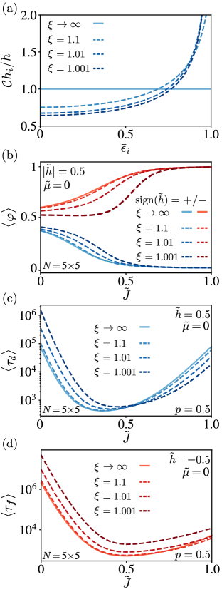
Figure E1: Comparison between a uniform and non-uniform force load. (a) The non-uniform force load distribution given by Eq. (E3) as a function of the normalized lattice distance $\bar{\epsilon}_{i}$. For $\xi<\infty$ adhesion bonds located at the outer edge of the lattice are subject to a larger external force than adhesion bonds located at the inner part of the lattice. (b) The equation of state for a pulling (blue) and pushing (red) force for various values of $\xi$ for a system of $N=5\times 5$ adhesion bonds with zero intrinsic binding-affinity. (c-d) The mean first passage time to dissolution (c) and formation (d) for mixed Glauber-Kawasaki dynamics with constant Glauber attempt probability $p=0.5$ under a pulling (blue) and pushing (red) force for various values of $\xi$ for a system of $N=5\times 5$ adhesion bonds with zero intrinsic binding-affinity.

In Fig. E1(b-d) we depict the equation of state (b) and mean first passage time to cluster dissolution (c) and formation (d) for mixed Glauber-Kawasaki dynamics with a constant Glauber attempt probability $p_{k}\rightarrow p=0.5$ and for various values of $\xi$ under a pulling or pushing force ($\tilde{h}=\pm 0.5$). The results were obtained by exact summation/algebraic techniques. Interestingly, for $\xi\geq 1.1$ the equation of state and mean first passage times are almost identical to the uniform force load solutions that correspond to $\xi\rightarrow\infty$. Only for $\xi<1.1$, which is valid for very large coupling values corresponding to extremely floppy membranes, we observe deviations from the uniform force results. The origin of the deviations is the extreme force load on the outer bonds, which is $\sqrt{\xi/(\xi-1)}$ times larger than the force load on the inner bond. For $\xi=1.01$ this leads approximately to a factor of $\times 10$, and for $\xi=1.001$ this leads approximately to a factor of $\times 32$. Hence, for most physically meaningful realizations of a non-uniform force distribution (i.e. distributions based on Eq. (E3)) the results converge to the uniform force solutions. Only under the extreme conditions where the force load on the outer bonds becomes at least an order of magnitude larger compared to the inner bonds we find large deviations from the uniform force load.

Note that the relative fraction of edge bonds in the limit of larger system sizes (and specifically in the thermodynamic limit) vanishes. Therefore we expect a non-uniform force load, which mainly penalizes the edge bonds for $\xi\rightarrow 1$, to have an even weaker effect on the equation of state and mean first passage times in large systems.

E.3 Proof of detailed-balance for local equilibrium rates

Before stating the explicit result for the mean first passage time to dissolution/formation in the local equilibrium approximation, we prove that the local equilibrium transition rates $\bar{w}_{k\to k\pm 1}$ given by Eq. (21) obey detailed-balance w.r.t $Q_{k}$ defined in Eq. (6). The effective transition rates are obtained by mapping the full mixed Glauber-Kawasaki dynamics onto an effective birth-death process over the number of closed bonds (see Fig. 6), where we assume that the dynamics reaches a local equilibrium at any number of closed bonds before any transition. As a result, the birth-death process is a Markov chain on the free energy landscape for the fraction of closed bonds $\varphi$. Recall that the original Glauber rates in Eq. (3) obey detailed-balance w.r.t. the Hamiltonian $\mathcal{H}(\{\sigma_{j}\})$, and therefore

$$\mathrm{e}^{-\beta\mathcal{H}(\{\sigma_{j}\})}\delta_{N_{c}(\{\sigma_{j}\}),k}w_{i}(\{\sigma_{j}\})\delta_{N_{c}(\{\sigma_{j}\}_{i}^{\prime}),k\pm 1}=\\ \mathrm{e}^{-\beta\mathcal{H}(\{\sigma_{j}\}_{i}^{\prime})}\delta_{N_{c}(\{\sigma_{j}\}_{i}^{\prime}),k\pm 1}w_{i}(\{\sigma_{j}\}_{i}^{\prime})\delta_{N_{c}(\{\sigma_{j}\}),k},$$ (E4)

where we have explicitly incorporated the constraints arising from single-bond-flip dynamics by means of the Kronecker delta´s. Upon summing the left hand side of Eq. (E4) over all initial configurations with $N_{c}(\{\sigma_{j}\})=k$ and over all rates that jump to a configuration with $N_{c}(\{\sigma_{j}\}_{i}^{\prime})=k\pm 1$, we reach all possible final configurations with $N_{c}(\{\sigma_{j}\}_{i}^{\prime})=k\pm 1$, with a backward rate given by the sum of all rates that jump to a configuration with $N_{c}(\{\sigma_{j}\})=k$. Hence we find the equality

$$\sum\limits_{\{\sigma_{j}\}}\sum\limits_{i=1}^{N}\mathrm{e}^{-\beta\mathcal{H}(\{\sigma_{j}\})}\delta_{N_{c}(\{\sigma_{j}\}),k}w_{i}(\{\sigma_{j}\})\delta_{N_{c}(\{\sigma_{j}\}_{i}^{\prime}),k\pm 1}=\\ \sum\limits_{\{\sigma_{j}\}_{i}^{\prime}}\sum\limits_{i=1}^{N}\mathrm{e}^{-\beta\mathcal{H}(\{\sigma_{j}\}_{i}^{\prime})}\delta_{N_{c}(\{\sigma_{j}\}_{i}^{\prime}),k\pm 1}w_{i}(\{\sigma_{j}\}_{i}^{\prime})\delta_{N_{c}(\{\sigma_{j}\}),k}.$$ (E5)

Comparing Eq. (E5) with Eq. (21), we recognize the left and right hand side as $\tilde{Q}_{k}\bar{w}_{k\to k\pm 1}$ and $\tilde{Q}_{k\pm 1}\bar{w}_{k\pm 1\to k}$, respectively, which proves the effective detailed-balance relation

$$\tilde{Q}_{k}\bar{w}_{k\to k\pm 1}=\tilde{Q}_{k\pm 1}\bar{w}_{k\pm 1\to k}.$$ (E6)

E.4 First passage time statistics within the local equilibrium approximation

The local equilibrium approximation maps the complete mixed Glauber-Kawasaki dynamics onto an effective birth-death process with a right-acting tri-diagonal transition matrix $\mathbf{P}^{\rm le}$ of size $(N+1)\times(N+1)$ with elements

$$P^{\rm le}_{ij}=\Lambda_{i}\delta_{ij}+\\ \bar{w}_{i-1\to i}\delta_{i+1j}\theta\left(N-i\right)+\bar{w}_{i-1\to i-2}\delta_{i-1j}\theta\left(i-2\right),$$ (E7)

and $\Lambda_{i}=1-\sum_{j\neq i}^{N+1}P^{\rm le}_{ij}$. To obtain the mean first passage time we use the same algebraic technique as for small clusters. Upon removing the first/last row and column of $\mathbf{P}^{\rm le}$ we obtain the submatrix $\mathbf{T}^{\rm le}_{\rm d,f}$ for cluster dissolution and formation, respectively. We can invert the tri-diagonal submatrix exactly, which leads to the following LU/UL decomposition

$$(\mathbf{1}-\mathbf{T}^{\rm le}_{\rm{d,f}})^{-1}=\mathcal{A}^{\rm{d,f}}\mathcal{B}^{\rm{d,f}},$$ (E8)

where $\mathcal{A}^{\rm{d}}$ and $\mathcal{B}^{\rm{d}}$ are the lower and upper triangular matrix with elements

$$\mathcal{A}^{\rm d}_{ij}=\frac{\theta\left(i-j\right)}{\tilde{Q}_{j-1}}\bar{w}_{j-1\rightarrow j},\ \ \mathcal{B}^{\rm d}_{ij}=\tilde{Q}_{j}\theta\left(j-i\right),$$ (E9)

and $\mathcal{A}^{\rm{f}}$ and $\mathcal{B}^{\rm{f}}$ are the upper and lower triangular matrix with elements

$$\mathcal{A}^{\rm f}_{ij}=\frac{\theta\left(j-i\right)}{\tilde{Q}_{j}}\bar{w}_{j\rightarrow j-1},\ \ \mathcal{B}^{\rm f}_{ij}=\tilde{Q}_{j-1}\theta\left(i-j\right).$$ (E10)

A proof that Eq. (E8) is indeed the inverse of $\mathbf{1}-\mathbf{T}^{\rm le}_{\rm{d,f}}$ is given in the SM. Let us denote with $\langle\tau^{\rm le}_{d,f}\rangle_{m}$ the mean first passage time to cluster dissolution and formation, starting from the state with $m$ closed bonds. Using Eq. (E8) we obtain an exact expression for the first moments

$$\langle\tau_{d}^{\rm le}\rangle_{0<m\leq N}=\mathbf{\hat{e}}_{m}^{T}\mathcal{A}^{\rm d}\mathcal{B}^{\rm d}\mathbf{e}=\sum_{k=0}^{m-1}\frac{1}{\bar{w}_{k\rightarrow k+1}}\sum_{l=k+1}^{N}\frac{\tilde{Q}_{l}}{\tilde{Q}_{k}},$$ (E11)

$$\langle\tau_{f}^{\rm le}\rangle_{0\leq m<N}=\mathbf{\hat{e}}_{m+1}^{T}\mathcal{A}^{\rm f}\mathcal{B}^{\rm f}\mathbf{e}=\sum_{k=m+1}^{N}\frac{1}{\bar{w}_{k\rightarrow k-1}}\sum_{l=0}^{k-1}\frac{\tilde{Q}_{l}}{\tilde{Q}_{k}},$$ (E12)

where $\mathbf{\hat{e}}_{m}$ is the column vector with dimension $N$ with components $(\mathbf{\hat{e}}_{m})_{i}=\delta_{mi}$, and $\mathbf{e}$ is the column vector with all components equal to 1. Notice that Eq. (E8), and therefore Eqs. (E11) and (E12), are applicable to any right-acting tri-diagonal transition matrix with rates obeying detailed-balance. Although we only present the mean first passage time here, we can easily obtain any higher order moments of the first passage time to cluster dissolution and formation using Eq. (E8) [78]. Notably, Eqs. (E11) and (E12) appear to have a similar structure as the largest eigenvalue of the transition matrix in classical nucleation theory [148, 120].

E.5 A bound on the effective transition rates

Here we present a bound on the local equilibrium rates given by Eq. (21) which proves that the transition rates are strictly sub-exponential in $N$. First, we consider a bound for the exit rates $w_{\rm exit}^{\pm}(\{\sigma_{i}\})$ defined in Eq. (22), which contain a sum over the original Glauber rates that are defined in Eq. (3). Since $1-\tanh{(x)}\geq 0\ \forall x\in\mathds{R}$ the Glauber rates are non-negative, and therefore the exit rates obey the bound

$$w^{\rm max}_{k\to k\pm 1}\leq w_{\rm exit}^{\pm}(\{\sigma_{i}\})\leq c^{\pm}_{k}w^{\rm max}_{k\to k\pm 1},$$ (E13)

with $c_{k}^{+}=N-k$ and $c_{k}^{-}=k$ denoting the number of terms inside the sum of Eq. (22), and $w^{\rm max}_{k\to k\pm 1}$ denotes the largest transition rate to go from a state with $k$ to $k\pm 1$ closed bonds. The largest transition rate can be written as

$$w^{\rm max}_{k\to k\pm 1}=\frac{1}{2N}\left[1-\tanh{(\Delta\mathcal{H}^{\rm min}_{k\to k\pm 1}/2)}\right],$$ (E14)

where

$$\Delta\mathcal{H}^{\rm min}_{k\to k\pm 1}\equiv\inf_{\begin{subarray}{c}N_{c}(\{\sigma_{j}\})=k,\\ N_{c}(\{\sigma_{j}\}_{i}^{\prime})=k\pm 1\end{subarray}}\{\mathcal{H}(\{\sigma_{j}\}_{i}^{\prime})-\mathcal{H}(\{\sigma_{j}\})\}$$ (E15)

denotes the smallest possible energy change between two configurations $\{\sigma_{j}\}$ and $\{\sigma_{j}\}_{i}^{\prime}$ with $N_{c}(\{\sigma_{j}\})=k$ and $N_{c}(\{\sigma_{j}\}_{i}^{\prime})=k\pm 1$, respectively. To obtain a closed-form expression for $w^{\rm max}_{k\to k\pm 1}$ we first note that the contribution to $\Delta\mathcal{H}^{\rm min}_{k\to k\pm 1}$ from the external force and intrinsic binding-affinity are fixed and given by the second and third term in Eq. (3). Therefore we are left to consider the smallest energy change due to the coupling strength, which we denote as $\Delta_{\tilde{J}}\mathcal{H}^{\rm min}_{k\to k\pm 1}$. For a square lattice with free boundary conditions the minimal energy “forward transitions” with energy difference $\Delta_{\tilde{J}}\mathcal{H}^{\rm min}_{k\to k+1}$ for various values of $k$ are depicted in Fig. (E2). Similarly, the minimal energy “downward transitions” with energy difference $\Delta_{\tilde{J}}\mathcal{H}^{\rm min}_{k\to k-1}$ are obtained by interchanging the open (red) and closed (green) adhesion pairs in Fig. (E2). Combining these two results yields $\Delta_{\tilde{J}}\mathcal{H}^{\rm min}_{k\to k\pm 1}=2m_{k}^{\pm}\tilde{J}$, with

$$m_{k}^{\pm}\equiv 2(c_{k}^{\mp}-1)\theta(2-c_{k}^{\mp})-\min(c_{k}^{\mp},4)\theta(c_{k}^{\mp}-3),$$ (E16)

and delivers the expression for $w^{\rm max}_{k\to k\pm 1}$. Finally, since $w^{\rm max}_{k\to k\pm 1}$ is independent of the specific configuration $\{\sigma_{i}\}$ at fixed $k$, it drops out of the sum over $\{\sigma_{i}\}$ in Eq. (21) for the effective transition rates, and therefore the bound in Eq. (E13) can directly be applied to the effective transition rate upon multiplying both sides with the Glauber attempt probability

$$p_{k}w^{\rm max}_{k\to k\pm 1}\leq\bar{w}_{k\to k\pm 1}\leq p_{k}c^{\pm}_{k}w^{\rm max}_{k\to k\pm 1},$$ (E17)

which yields the bound on the effective transition rate.

The lower and upper bound for the effective transition rate are used to determine an upper and lower bound for the mean first passage time to cluster dissolution and formation, respectively. The specific result for a rectangular lattice of size $N=6\times 7$ for pure Glauber dynamics (i.e. $p_{k}=1\ \forall k$) is shown in Fig. E3. For small values of the coupling strength $\tilde{J}$ we find that the upper bound in Eq. (E17), corresponding to the lower bound in Fig. E3 (since $\langle{\rm t}_{{\rm d,f}}\rangle\propto 1/\bar{w}_{k\to k\pm 1}$), is saturated by the exact effective transition rate. Conversely, for large values of the coupling strength it seems that the lower bound in Eq. (E17) is saturated.

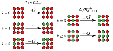
Figure E2: Minimum energy forward transitions between two configurations $\{\sigma_{j}\}$ and $\{\sigma_{j}\}_{i}^{\prime}$ with $N_{c}(\{\sigma_{j}\})=k$ and $N_{c}(\{\sigma_{j}\}_{i}^{\prime})=k+1$ respectively. Although we depict here the minimal energy differences for a lattice of size $N=3\times 3$, the result holds for any two-dimensional lattice of size $N\geq 3\times 3$ as long as the transitions for $k=0,1,2$ are taken at the corner, and the transition for $k=3$ is taken at the edge.

E.6 Approximate effective transition rate

For systems larger than $N\approx 50$ bonds the combinatorics involved in the computation of $Q_{k}$ defined in Eq. (6) and $\bar{w}_{k\to k+1}$ in Eq. (21) become prohibitive, and thus forces us to make further approximations. To get Eq. (23) fully explicit we make an “instanton” approximation for $\bar{w}_{k\to k\pm 1}$ using the Bethe-Guggenheim approximation with the bound given by Eq. (E17), and reads

$$\bar{w}_{k\to k\pm 1}\approx\max(1,\alpha_{k}c_{k}^{\pm})p_{k}w^{\rm max}_{k\to k\pm 1},$$ (E18)

with $\alpha_{k}=\delta_{k0}+\delta_{kN}+2\bar{X}_{k}/N\in\left[0,1\right]$, $c_{k}^{+}=N-k$, $c_{k}^{-}=k$, and $\bar{X}_{k}$ given by Eq. (9). The prefactor $\alpha_{k}c_{k}^{\pm}$ is a measure for the number of ”favorable” adhesion bonds that are most likely to flip in a configuration with $k$ closed bonds. For $k=0\lor N$ all bonds have an equal surrounding in the thermodynamic limit (or for a periodic lattice), and therefore all $c_{k}^{\pm}$ open/closed bonds are equally likely to attempt a flip. For $0<k<N$ it becomes energetically more favorable to flip a bond which is part of an open-closed adhesion pair (see Fig. E2). To determine the number of bonds that constitute an open-closed pair, we recall that $\bar{z}\bar{X}_{k}$ is a measure for the number of open-closed pairs in a lattice of size $N$ with $k$ closed bonds. Upon dividing by the total number of pairs in the system, given by $\bar{z}N/2$, we obtain the probability to select an open-closed pair in the lattice that is given by

$$\frac{2\bar{X}_{k}}{N}=\frac{4X^{*}_{k}/N}{\left[1+4X^{*}_{k}(\mathrm{e}^{4\tilde{J}}-1)/N\right]^{\frac{1}{2}}+1},$$ (E19)

where $4X^{*}_{k}/N=4k(N-k)/N^{2}\in\left[0,1\right]$. Multiplying Eq. (E19) by the total number of open/closed adhesion bonds, i.e. $2c_{k}^{\pm}\bar{X}_{k}/N$, we obtain an approximate expression for the number of open/closed bonds which constitute an open-closed adhesion pair.

To prove that the approximate effective rate given by Eq. (E18) obeys the bound given by Eq. (E17) we apply a chain of inequalities. First we note that $0\leq 2\bar{X}_{k}/N\leq 1/2$, where the upper bound follows from considering $\tilde{J}=0$ and $k=N/2$ in Eq. (E19), and the lower bound is given for $k=0\lor N$ or the limit $\tilde{J}\to\infty$. From this it follows that $0\leq\alpha_{k}\leq 1$, and therefore $1\leq\max(1,\alpha_{k}c_{k}^{\pm})\leq c^{\pm}_{k}$. Finally, since we use $p_{k}w^{\rm max}_{k\to k\pm 1}$ in Eq. (E18), it cancels on both sides of the inequality in Eq. (E17), which leaves to prove the inequality we have proven above and thereby completes the proof.

Fig. E3 shows the mean first passage time to cluster dissolution and formation obtained with the approximate effective rates (E18) in combination with the Bethe-Guggenheim approximation for $Q_{k}$ for a lattice of size $N=6\times 7$ for pure Glauber dynamics (i.e. $p_{k}=1\ \forall k$). The results obtained with the approximate rates (black symbols) agree to a high degree with the results obtained by the exact effective rates (blue solid line).

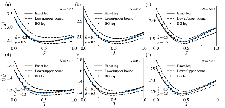
Figure E3: Comparison of the exact local equilibrium effective rates and the approximate Bethe-Guggenheim local equilibrium effective rates for pure Glauber dynamics. $\langle{\rm t}_{\rm d,f}\rangle$ for cluster dissolution (a)-(c) and cluster formation (d)-(f) as a function of the coupling $\tilde{J}$ for fixed intrinsic binding-affinity $\tilde{\mu}=0.5$ in the presence of a pushing force $\tilde{h}=-0.3$ (a and d), zero force $\tilde{h}=0$ (b and e), and a pulling force $\tilde{h}=0.3$ (c and f); The blue solid line is obtained with the exact local equilibrium effective transition rate and exact partition function $Q_{k}$ (Eqs. (21) and (6), respectively) with $p_{k}=1\ \forall k$. The black symbols are obtained with the Bethe-Guggenheim approximation to the effective rate and partition function $Q_{k}^{\rm BG}$ (Eqs. (21) and (6) in combination with Eq. (8), respectively). The black dotted line indicates the upper and lower bound to the mean dissolution/formation time, which is obtained with the upper and lower bound to the effective transition rate in combination with the exact partition function (Eqs. (E17) and (6) respectively).

E.7 The mean first passage time in the thermodynamic limit

Here we prove the result for the mean first passage time to dissolution/formation in the thermodynamic limit given by Eqs. (24) and (25) based on the local equilibrium approximation. Intuitively $\langle\tau_{d,f}\rangle$ must scale as $\langle\tau_{d,f}\rangle\sim\mathrm{e}^{N\Delta\tilde{\rm f}^{\dagger}}$, where $\Delta\tilde{\rm f}^{\dagger}\equiv\tilde{\rm f}_{\rm max}-\tilde{\rm f}_{\rm min}$ denotes the difference in the free energy density between the minimum, $\tilde{\rm f}_{\rm min}=\inf_{\varphi}\tilde{\rm f}(\varphi)$, and the maximum, $\tilde{\rm f}_{\rm max}\equiv\sup_{\varphi}\tilde{\rm f}(\varphi)$, that for large clusters becomes independent of $N$. Indeed, according to Eq. (23) we have $\tilde{Q}_{l}/\tilde{Q}_{k}=(p_{k}/p_{l})\mathrm{e}^{N[\tilde{f}_{N}(k/N)-\tilde{f}_{N}(l/N)]}$ and recall that $\bar{w}_{k\to k+1}$ is strictly sub-exponential in $N$. Furthermore we make the assumption that the Glauber attempt probabilities $p_{k}$ are strictly sub-exponential in $N$. Since both series in Eq. (23) are absolutely convergent, we can apply a version of the “squeeze” theorem to Eq. (23).

To simplify the notation we write the summands in Eq. (23) as $0<(p_{k}/p_{l})a_{k,l}/\bar{w}_{k\to k+1}<\infty$, where $a_{k,l}\equiv\mathrm{e}^{N[\tilde{f}_{N}(k/N)-\tilde{f}_{N}(l/N)]}$. If $k^{\dagger}$ denotes the index of the largest $k$-dependent term

$$k^{\dagger}\equiv\sup_{0\leq k<N}\frac{p_{k}\exp[N\tilde{f}_{N}(k/N)]}{\bar{w}_{k\to k+1}}$$ (E20)

and by $l_{d,f}^{\dagger}$ the index of the largest l-dependent term

$$l_{d}^{\dagger} \equiv \sup_{k^{\dagger}<l\leq N}\frac{\exp{[-N\tilde{f}_{N}(l/N)]}}{p_{l}},$$

$$l_{f}^{\dagger} \equiv \sup_{0<l<k^{\dagger}}\frac{\exp{[-N\tilde{f}_{N}(l/N)]}}{p_{l}},$$ (E21)

then the following chain of inequalities holds for any $N$

$$\frac{p_{k^{\dagger}}a_{k^{\dagger},l^{\dagger}_{d,f}}}{p_{l^{\dagger}_{d,f}}\bar{w}_{k^{\dagger}\to k^{\dagger}+1}}\leq\sum_{k=0}^{N-1}\!\sum_{l=m}^{M-1}\!\frac{p_{k}a_{k,l}}{p_{l}\bar{w}_{k\to k+1}}\leq\frac{c_{M,m}p_{k^{\dagger}}a_{k^{\dagger},l^{\dagger}_{d,f}}}{p_{l^{\dagger}_{d,f}}\bar{w}_{k^{\dagger}\to k^{\dagger}+1}},$$ (E22)

where $c_{M,m}\equiv N(M-m)$, $M=N+1$ and $m=k+1$ for dissolution, and $M=k+1$ and $m=0$ for cluster formation. Since $x^{1/N}$ is monotonic in $x>0$, such that $x_{1}<x_{2}$ implies $x_{1}^{1/N}<x_{2}^{1/N}$, the inequality (E22) is preserved when exponentiated to $1/N$. The thermodynamic limit of Eq. (E22) is a scaling limit, i.e. $\lim_{s}\equiv\lim_{N\to\infty}|_{k/N=\varphi_{k}}^{l/N=\varphi_{l}}$, and thus the inequality (E22) becomes

$${\rm lim}_{s}\!\left[\frac{p_{k^{\dagger}}a_{k^{\dagger},l^{\dagger}_{d,f}}}{p_{l^{\dagger}_{d,f}}\bar{w}_{k^{\dagger}\to k^{\dagger}+1}}\right]^{\!\frac{1}{N}}\leq\langle{\rm t_{d,f}}\rangle\leq\mathrm{lim}_{s}\!\left[\frac{c_{M,m}p_{k^{\dagger}}a_{k^{\dagger},l^{\dagger}_{d,f}}}{p_{l^{\dagger}_{d,f}}\bar{w}_{k^{\dagger}\to k^{\dagger}+1}}\right]^{\!\frac{1}{N}}\!\!\!\!.$$ (E23)

Moreover, since ${\rm lim}_{s}\,\bar{w}^{-1/N}_{k^{\dagger}\to k^{\dagger}+1}=1$, ${\rm lim}_{s}\,[c_{M,m}]^{1/N}=1$, and ${\rm lim}_{s}\,[p_{k^{\dagger}}/p_{l^{\dagger}_{d,f}}]^{1/N}=1$, all four limits in Eq. (E23) exist and thus may be taken separately, implying the convergence of the upper bound in Eq. (E23) to the lower bound. Thereby $\langle{\rm t_{d,f}}\rangle$ becomes squeezed in-between rendering the inequality an equality. Since $\lim_{s}\tilde{f}_{N}(k^{\dagger}/N)=\tilde{\rm f}(\varphi_{\rm max})$ and $\lim_{s}\tilde{f}_{N}(l_{d,f}^{\dagger}/N)=\tilde{\rm f}(\varphi^{d,f}_{\rm min})$ we finally obtain Eqs. (24) and (25), thus completing the proof.

E.8 Evaluation of the Bethe-Guggenheim mean first passage time in the thermodynamic limit

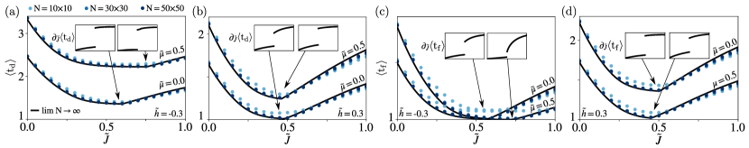
Figure E4: Master scaling of mean dissolution and formation times per bond for finite clusters and in the thermodynamic limit. $\langle{\rm t_{d,f}}\rangle$ for cluster dissolution (a-b) and formation (c-d) as a function of the coupling $\tilde{J}$ for a pair of intrinsic affinities $\tilde{\mu}=0$ and $\tilde{\mu}=0.5$ and various cluster sizes (symbols) as well as the thermodynamic limit (lines) in the presence of an external pushing (a,c) and pulling (b,d) force; Symbols are evaluated with local equilibrium approximation Eqs. (23) using $Q_{k}^{\rm BG}$ (Eqs. (6) and (8)) and $\bar{w}_{k\to k+1}$ from Eq. (E18) with $p_{k}=1\ \forall k$ (i.e. pure Glauber dynamics)

. The discrepancy between the lines and symbols is due to finite-size effects.

In the previous section we have proven that in the thermodynamic limit the mean first passage time to cluster dissolution/formation scales as $\langle\tau_{d,f}\rangle\simeq\langle\rm{t}_{\rm d,f}\rangle^{N}=\mathrm{e}^{N\Delta\tilde{\rm f}^{\dagger}}$, where $\Delta\tilde{\rm f}^{\dagger}$ denotes the largest left/right barrier in the Bethe-Guggenheim free energy density Eq. (12). In this section we determine $\Delta\tilde{\rm f}^{\dagger}$ and thereby obtain a closed-form expression for the mean first passage time per bond in the thermodynamic limit.

E.8.1 Case 1: $\tilde{J}\geq 0$, $\tilde{h}=\tilde{\mu}=0$

We first consider the mean first passage time to cluster dissolution/formation in the absence of an external force and intrinsic binding-affinity. Due to the $\mathds{Z}_{2}$ symmetry of the coupling strength, we note that $\langle\rm t_{d}\rangle=\langle\rm t_{f}\rangle$. Our first task is to find the locations of the global maximum and minimum in the free energy landscape, denoted by $\varphi^{d,f}_{\rm max}$ and $\varphi^{d,f}_{\rm min}$, respectively.

The position of the global minimum for zero force and intrinsic binding-affinity is given by Eq. (D14), while the position of the global maximum is located at $\varphi^{d,f}_{\rm max}=0\land 1$ for low values of the coupling strength $\tilde{J}$, and at $\varphi^{d,f}_{\rm max}=1/2$ for large values. The coupling strength at which the global maximum changes position corresponds to the root of the equation

$$\tilde{\rm f}\left(0\right)-\tilde{\rm f}\left(\frac{1}{2}\right)=\frac{\bar{z}}{2}\ln{\left(\mathrm{e}^{2\tilde{J}}+1\right)}-\bar{z}\tilde{J}+\left(1-\frac{\bar{z}}{2}\right)\ln{\left(2\right)},$$ (E24)

which is given by

$$\tilde{J}^{\rm d}_{\rm crit,BG}=-\frac{1}{2}\ln{\left(2^{1-2/\bar{z}}-1\right)},$$ (E25)

and sets the dynamical critical coupling value for the zero-field Ising model under the Bethe-Guggenheim approximation.

Surprisingly, for the two-dimensional square lattice with $\bar{z}=4$ we exactly recover the static critical point obtained by Onsager [83]. To check whether this is a mere coincidence we note that for the honeycomb lattice with $\bar{z}=3$ the exact statical critical point is given by $\tilde{J}^{\rm s}_{\rm crit}=\frac{1}{2}\ln{\left(2+\sqrt{3}\right)}=0.65...$ [149], whereas Eq. (E25) gives $\tilde{J}^{\rm d}_{\rm crit}=\frac{-1}{2}\ln{\left(2^{1/3}-1\right)}=0.67...$, and so we find direct evidence that the dynamical critical point in the Bethe-Guggenheim approximation does not (at least not always) coincide with the exact statical critical point.

Combining our results for the locations of the global maximum and minimum we obtain the following result for the mean first passage time per adhesion bond in the thermodynamic limit for the zero field Ising model on a two-dimensional square lattice

$$\ln\langle{\rm t_{d,f}}\rangle=\left\{\begin{array}[]{lc}\tilde{\rm f}(0)-\tilde{\rm f}(\frac{1}{2}),&0\leq\tilde{J}\leq\tilde{J}^{\rm s}_{\rm crit,BG}\\ \tilde{\rm f}(0)-\tilde{\rm f}(\frac{1}{2}[1\pm\mathcal{C}]),&\tilde{J}^{\rm s}_{\rm crit,BG}\leq\!\tilde{J}\!\leq\tilde{J}^{\rm d}_{\rm crit,BG}\\ \tilde{\rm f}(\frac{1}{2})-\tilde{\rm f}(\frac{1}{2}[1\pm\mathcal{C}]),&\tilde{J}\geq\tilde{J}^{\rm d}_{\rm crit,BG},\end{array}\right.$$ (E26)

where $\mathcal{C}\equiv\mathrm{e}^{2\tilde{J}}\sqrt{\mathrm{e}^{4\tilde{J}}-4}/(\mathrm{e}^{4\tilde{J}}-2)$ comes from Eq. (D14), $\tilde{J}^{\rm s}_{\rm crit}=\ln{(2)}/2$ denotes the statical critical point for zero force, and $\tilde{J}^{\rm d}_{\rm crit}=\ln{(1+\sqrt{2})}/2$ the dynamical critical point in the force free case. This ultimately leads to Eq. (29) in the main text.

In the strong coupling limit we find from Eq. (E26) $\lim_{\tilde{J}\to\infty}\langle{\rm t}_{\rm d,f}\rangle=2$, which is identical to the result obtained for zero coupling. The physical intuition behind this result comes from considering the average number of steps required to change the state of a single independent adhesion bond. For zero force and intrinsic binding-affinity the probability to associate/dissociate is a $1/2$, and therefore the average dissolution/formation time is given by

$$1\left(\frac{1}{2}\right)+2\left(\frac{1}{2}\right)^{2}+3\left(\frac{1}{2}\right)^{3}+...=\sum\limits_{n=1}^{\infty}n\left(\frac{1}{2}\right)^{n}=2.$$

For an infinite coupling strength the interaction between the bonds is so strong that effectively the system behaves as one “super bond”, and therefore the average dissolution/formation time is equal to that of a single independent adhesion bond.

E.8.2 Case 2: $\tilde{J}\geq 0$, $\tilde{\mu}\neq 0$, $\tilde{h}=0$

Here we use the results obtained in Appendix D which leads to

$$\ln\langle{\rm t}_{\rm d}\rangle=\left\{\begin{array}[]{lc}\tilde{\rm f}\left(0\right)-\tilde{\rm f}\left(\varphi_{1}\right),&0\leq\tilde{J}\leq\ln{\min{\{\sqrt{2},s_{0}\}}}\\ \tilde{\rm f}\left(0\right)-\tilde{\rm f}\left(\varphi_{3}\right),&\ln{\min{\{\sqrt{2},s_{0}\}}}\leq\tilde{J}\leq\tilde{J}^{\rm d,-}_{\rm crit}\\ \tilde{\rm f}\left(\varphi_{4}\right)-\tilde{\rm f}\left(\varphi_{3}\right),&\tilde{J}\geq\tilde{J}^{\rm d,-}_{\rm crit}\end{array},\right.$$ (E27)

for cluster dissolution, and

$$\ln\langle{\rm t}_{\rm f}\rangle=\left\{\begin{array}[]{lc}\tilde{\rm f}\left(1\right)-\tilde{\rm f}\left(\varphi_{1}\right),&0\leq\tilde{J}\leq\ln{\min{\{\sqrt{2},s_{0}\}}}\\ \tilde{\rm f}\left(1\right)-\tilde{\rm f}\left(\varphi_{3}\right),&\ln{\min{\{\sqrt{2},s_{0}\}}}\leq\tilde{J}\leq\tilde{J}^{\rm d,+}_{\rm crit}\\ \tilde{\rm f}\left(\varphi_{4}\right)-\tilde{\rm f}\left(\varphi_{1}\right),&\tilde{J}\geq\tilde{J}^{\rm d,+}_{\rm crit}\end{array}\right.,$$ (E28)

for cluster formation, where $\varphi_{i}=\xi_{i}^{4}/(1+\xi_{i}^{4})$ is given by Eqs. (D7a) and (D7b), $s_{0}\equiv\sqrt{2\sqrt{2}}\mathrm{e}^{-\tilde{\mu}/4}$, and $\tilde{J}^{\rm d,-}_{\rm crit}$ and $\tilde{J}^{\rm d,+}_{\rm crit}$ are the dynamical critical points for cluster dissolution and formation respectively, which are solutions of

$$[\tilde{\rm f}\left(0\right)-\tilde{\rm f}\left(\varphi_{4}\right)]|_{\tilde{J}^{\rm d,-}_{\rm crit}}\stackrel{{\scriptstyle!}}{{=}}0,$$ (E29a)

$$[\tilde{\rm f}\left(1\right)-\tilde{\rm f}\left(\varphi_{3}\right)-\tilde{\rm f}\left(\varphi_{4}\right)+\tilde{\rm f}\left(\varphi_{1}\right)]|_{\tilde{J}^{\rm d,+}_{\rm crit}}\stackrel{{\scriptstyle!}}{{=}}0.$$ (E29b)

E.8.3 Case 3: $\tilde{J}\geq 0$, $\tilde{\mu}\neq 0$, $\tilde{h}\neq 0$

Using a quadratic Newton series (which is defined in Appendix D), Eqs. (E27) and (E28) are directly applicable to the non-zero force scenario upon applying the transformation $\varphi_{i}\to\varphi^{*}_{i}$, where $\varphi^{*}_{i}=\xi^{*4}_{i}/(1+\xi^{*4}_{i})$ and

$$\xi^{*}_{i}=\xi_{i}-\frac{g^{\left(1\right)}\left(\xi_{i}\right)\pm\sqrt{g^{\left(1\right)}\left(\xi_{i}\right)^{2}-2g^{\left(0\right)}\left(\xi_{i}\right)g^{\left(2\right)}\left(\xi_{i}\right)}}{g^{\left(2\right)}\left(\xi_{i}\right)},$$ (E30)

with a minus sign for the global minimum $\xi^{*}_{1,3}$, and a plus sign for the global maximum $\xi^{*}_{4}$. The function $g^{(0)}(\xi)$ and its first and second derivative $g^{(1,2)}(\xi)$ are given in Eqs. (D6),(D22), and (D23), respectively.

Our analytical results for the mean first passage time to cluster dissolution and formation per adhesion bond are depicted in Fig. 8 and Fig E4 for zero and nonzero external force respectively; note the remarkable agreement between the black solid line depicting the thermodynamic limit and the results for finite system sizes on the order of $N\geq 10\times 10$.

E.9 Evaluation of the mean first passage time in the thermodynamic limit in the mean field approximation

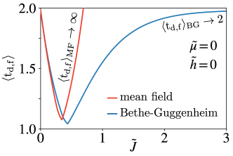
Figure E5: Mean dissolution/formation time in the thermodynamic limit: Bethe-Guggenheim versus mean field approximation. The Bethe-Guggenheim approximation is given by Eq. (E26), and the mean field approximation is given by Eq. (E35), where we solve for Eq. (E31) numerically.

Similarly to our previous analysis we must determine the global minimum and maximum, respectively, of the mean field free energy density given by Eq. (C2). For convenience we here consider only zero force and zero binding-affinity.

Below the statical critical coupling $\tilde{J}^{\rm s}_{\rm crit,MF}=1/\bar{z}$ there is a unique global minimum located at $\varphi^{d,f}_{\rm min}=1/2$. Above the statical critical coupling there exist two global minima, which are given by the non-zero solutions of the transcendental mean field equation

$$s=\tanh{\left(\bar{z}\tilde{J}s\right)},$$ (E31)

with $s=2\varphi-1$. Eq. (E31) is obtained directly from Eq. (C3) by using the relation $\ln{|\frac{1+x}{1-x}|}=2\tanh^{-1}{x}$.

Similarly to the Bethe-Guggenheim free energy density, the position of the global maximum is located at $\varphi^{d,f}_{\rm max}=0\land 1$ for small values of the coupling strength $\tilde{J}$, and at $\varphi^{d,f}_{\rm max}=1/2$ for large values. The transition at which the global maximum changes location is given by the root of the equation

$$\tilde{\rm f^{MF}}\left(0\right)-\tilde{\rm f^{MF}}\left(\frac{1}{2}\right)=-\frac{1}{2}\tilde{J}\bar{z}+\ln{(2)},$$ (E32)

which is given by

$$\tilde{J}^{\rm d}_{\rm crit,MF}=\frac{2}{\bar{z}}\ln{(2)},$$ (E33)

and sets the mean field dynamical critical coupling. For $\bar{z}=4$ we coincidentally recover the Bethe-Guggenheim statical critical coupling.

Combining our results for the locations of the global minimum and maximum we obtain the following results for the mean first passage time to cluster dissolution and formation per bond

$$\ln\langle{\rm t_{d,f}}\rangle_{\rm MF}=\left\{\begin{array}[]{lc}\tilde{\rm f^{MF}}(0)-\tilde{\rm f^{MF}}(\frac{1}{2}),&0\leq\tilde{J}\leq\frac{1}{\bar{z}}\\ \tilde{\rm f^{MF}}(0)-\tilde{\rm f^{MF}}(\frac{1}{2}[1\pm s]),&\frac{1}{\bar{z}}\leq\!\tilde{J}\!\leq\frac{2}{\bar{z}}\ln{(2)}\\ \tilde{\rm f^{MF}}(\frac{1}{2})-\tilde{\rm f^{MF}}(\frac{1}{2}[1\pm s]),&\tilde{J}\!\geq\frac{2}{\bar{z}}\ln{(2)},\end{array},\right.$$ (E34)

where $s$ is the non-zero solution of Eq. (E31). Evaluating Eq. (E34) explicitly using Eq. (C2) we find

$$\langle{\rm t_{d,f}}\rangle_{\rm MF}=\left\{\begin{array}[]{lc}2\mathrm{e}^{-\bar{z}\tilde{J}/2},&0\leq\tilde{J}\leq\frac{1}{\bar{z}}\\ 2\mathrm{e}^{-\bar{z}\tilde{J}(1-s^{2})/2}\lambda(s),&\frac{1}{\bar{z}}\leq\!\tilde{J}\!\leq\frac{2}{\bar{z}}\ln{2}\\ \mathrm{e}^{\bar{z}\tilde{J}s^{2}/2}\lambda(s),&\tilde{J}\!\geq\frac{2}{\bar{z}}\ln{(2)},\end{array}\right.$$ (E35)

where

$$\lambda(s)\equiv\frac{\exp(-s\operatorname{arctanh}{(s)})}{\sqrt{1-s^{2}}}=\frac{\exp(-\bar{z}\tilde{J}s^{2})}{\sqrt{1-s^{2}}},$$ (E36)

and in the second equality we used Eq. (C2) to make the substitution $\operatorname{arctanh}{(s)}=\bar{z}\tilde{J}s$.

As with the Bethe-Guggenheim analysis, we find a global minimum of $\langle{\rm t}_{\rm d,f}\rangle_{\rm MF}$ at the dynamical critical coupling given by

$$\langle{\rm t}_{\rm d,f}\rangle_{\rm MF}|_{\tilde{J}=\frac{2}{\bar{z}}\ln{(2)}}=\frac{\exp{(-\ln{(2)}s_{\rm crit}^{2})}}{\sqrt{1-s^{2}_{\rm crit}}}=1.0785(1),$$ (E37)

where $s_{\rm crit}$ is the solution of the transcendental equation $s_{\rm crit}=\tanh{(2\ln{(2)}s_{\rm crit})}$. Remarkably, the minimum for $\langle{\rm t}_{\rm d,f}\rangle_{\rm MF}$ is independent of the coordination number $\bar{z}$, and therefore the mean field approximation predicts a universal lower bound on the mean first passage time to cluster dissolution and formation per bond.

At the dynamical critical coupling there is a first-order discontinuity w.r.t. the coupling $\tilde{J}$ given by

$$\lim_{\tilde{J}\nearrow\frac{2}{\bar{z}}\ln(2)}\partial_{\tilde{J}}\langle{\rm t_{d,f}}\rangle = -\frac{\bar{z}}{2}(1-s^{2}_{\rm crit})\langle{\rm t}_{\rm d,f}\rangle_{\rm MF}|_{\tilde{J}=\frac{2}{\bar{z}}\ln{(2)}}$$

$$\lim_{\tilde{J}\searrow\frac{2}{\bar{z}}\ln(2)}\partial_{\tilde{J}}\langle{\rm t_{d,f}}\rangle = \frac{\bar{z}}{2}s^{2}_{\rm crit}\langle{\rm t}_{\rm d,f}\rangle_{\rm MF}|_{\tilde{J}=\frac{2}{\bar{z}}\ln{(2)}},$$ (E38)

where we use Eq. (E37). The derivatives have a trivial dependence on $\bar{z}$ while the ratios of the two derivatives are independent of $\bar{z}$.

In the range $1/\bar{z}<\tilde{J}<\infty$ we need to solve Eq. (E31) numerically to get Eq. (E35) fully explicit. In the limit $\tilde{J}\rightarrow\infty$ Eq. (E31) translates to

$$s=\theta\left(s\right)-\theta\left(-s\right),$$ (E39)

where $\theta\left(s\right)=1$ for $s\geq 0$ and zero otherwise. The two non-zero solutions of Eq. (E39) are given by $s=\pm 1$, corresponding to $\varphi=0,1$. Finally we use that $\lim_{s\to\pm 1}\lambda(s)=1/2$ to find

$$\lim\limits_{\tilde{J}\rightarrow\infty}\langle{\rm t}_{\rm d,f}\rangle_{\rm MF}=\lim\limits_{\tilde{J}\rightarrow\infty}\frac{1}{2}\exp{\left(\frac{\bar{z}\tilde{J}}{2}\right)}=\infty\ \forall\bar{z}>0.$$ (E40)

The mean field approximation thus predicts unphysical dynamics in the strong coupling limit, which is also depicted in Fig. E5. The consideration of correlations is required in order to arrive at a physically correct and consistent result. It is therefore paramount to go beyond the mean field approximation and consider correlations explicitly.

In this Supplemental Material we prove the expression for the inverse of the matrix $\mathbf{1}-\mathbf{T}^{\rm le}_{\rm d,f}$ used in Appendix E4, where $\mathbf{T}^{\rm le}_{\rm d,f}$ is the sub-matrix for cluster dissolution/formation, The elements of $\mathbf{1}-\mathbf{T}^{\rm le}_{\rm d,f}$ are given by

$$\left[1-T^{\rm le}_{\rm d}\right]_{ij}=\Lambda^{\rm d}_{i}\delta_{ij}-\bar{w}_{i\to i+1}\delta_{i+1j}\theta\left(N-1-i\right)-\bar{w}_{i\to i-1}\delta_{i-1j}\theta\left(i-2\right),$$ (S1)

$$\left[1-T^{\rm le}_{\rm f}\right]_{ij}=\Lambda^{\rm f}_{i}\delta_{ij}-\bar{w}_{i-1\to i}\delta_{i+1j}\theta\left(N-1-i\right)-\bar{w}_{i-1\to i-2}\delta_{i-1j}\theta\left(i-2\right),$$ (S2)

where $\Lambda^{\rm d}_{i}=-\sum_{j\neq i}^{N}\left[1-T^{\rm le}_{\rm d}\right]_{ij}+\bar{w}_{1\to 0}\delta_{i1}$ and $\Lambda^{\rm f}_{i}=-\sum_{j\neq i}^{N}\left[1-T^{\rm le}_{\rm f}\right]_{ij}+\bar{w}_{N-1\to N}\delta_{iN}$. The inverse can be expressed as

$$\mathcal{N}_{\rm d,f}\equiv(\mathbf{1}-\mathbf{T}^{\rm le}_{\rm{d,f}})^{-1}=\mathcal{A}^{\rm{d,f}}\mathcal{B}^{\rm{d,f}},$$ (S3)

where $\mathcal{A}^{\rm{d}}$ and $\mathcal{B}^{\rm{d}}$ are the lower and upper triangular matrix, respectively, with elements

$$\mathcal{A}^{\rm d}_{ij}=\frac{\theta\left(i-j\right)}{{\color[rgb]{0,0,0}\tilde{Q}_{j-1}}\bar{w}_{j-1\rightarrow j}},\ \ \mathcal{B}^{\rm d}_{ij}={\color[rgb]{0,0,0}\tilde{Q}_{j}}\theta\left(j-i\right),$$ (S4)

and $\mathcal{A}^{\rm{f}}$ and $\mathcal{B}^{\rm{f}}$ are the upper and lower triangular matrix, respectively, with elements

$$\mathcal{A}^{\rm f}_{ij}=\frac{\theta\left(j-i\right)}{{\color[rgb]{0,0,0}\tilde{Q}_{j}}\bar{w}_{j\rightarrow j-1}},\ \ \mathcal{B}^{\rm f}_{ij}={\color[rgb]{0,0,0}\tilde{Q}_{j-1}}\theta\left(i-j\right),$$ (S5)

and $\tilde{Q}_{j}\equiv Q_{j}/p_{j}$ where $p_{j}$ is the Glauber attempt probability and $Q_{j}$ the partition function constrained to $j$, the number of closed bonds defined in Eq. (6). To prove that Eq. (S3) is the inverse of $\mathbf{1}-\mathbf{T}_{\rm d,f}$ we evaluate the corresponding matrix product. We first write the elements of the fundamental matrices as

$$\left[\mathcal{N}_{\rm d}\right]_{ij}=\sum\limits_{k=1}^{N}\mathcal{A}^{\rm d}_{ik}\mathcal{B}^{\rm d}_{kj}=\sum\limits_{k=1}^{N}\frac{{\color[rgb]{0,0,0}\tilde{Q}_{j}}\theta\left(i-k\right)\theta\left(j-k\right)}{{\color[rgb]{0,0,0}\tilde{Q}_{k-1}}\bar{w}_{k-1\rightarrow k}}=\sum\limits_{k=1}^{\min{\left(i,j\right)}}\frac{{\color[rgb]{0,0,0}\tilde{Q}_{j}}}{{\color[rgb]{0,0,0}\tilde{Q}_{k-1}}\bar{w}_{k-1\rightarrow k}},$$ (S6)

and

$$\left[\mathcal{N}_{\rm f}\right]_{ij}=\sum\limits_{k=1}^{N}\mathcal{A}^{\rm f}_{ik}\mathcal{B}^{\rm f}_{kj}=\sum\limits_{k=1}^{N}\frac{{\color[rgb]{0,0,0}\tilde{Q}_{j-1}}\theta\left(k-i\right)\theta\left(k-j\right)}{{\color[rgb]{0,0,0}\tilde{Q}_{k}}\bar{w}_{k\rightarrow k-1}}=\sum\limits_{k=\max{\left(i,j\right)}}^{N-1}\frac{{\color[rgb]{0,0,0}\tilde{Q}_{j-1}}}{{\color[rgb]{0,0,0}\tilde{Q}_{k}}\bar{w}_{k\rightarrow k-1}}.$$ (S7)

For cluster dissolution, the matrix product is given by

$$\sum\limits_{j=1}^{N}\left[1-T^{\rm le}_{\rm d}\right]_{ij}\left[\mathcal{N}_{\rm d}\right]_{jk}=\left[1-T^{\rm le}_{\rm d}\right]_{ii-1}\left[\mathcal{N}_{\rm d}\right]_{i-1k}\theta\left(i-2\right)+\left[1-T^{\rm le}_{\rm d}\right]_{ii}\left[\mathcal{N}_{\rm d}\right]_{ik}+\left[1-T^{\rm le}_{\rm d}\right]_{ii+1}\left[\mathcal{N}_{\rm d}\right]_{i+1k}\theta\left(N-1-i\right)=\\ \bar{w}_{i\rightarrow i-1}\left(\left[\mathcal{N}_{\rm d}\right]_{ik}-\left[\mathcal{N}_{\rm d}\right]_{i-1k}\theta\left(i-2\right)\right)+\bar{w}_{i\rightarrow i+1}\left(\left[\mathcal{N}_{\rm d}\right]_{ik}-\left[\mathcal{N}_{\rm d}\right]_{i+1k}\right)\theta\left(N-1-i\right).$$ (S8)

The difference between two consecutive elements of the fundamental matrix can be obtained from Eq. (S6), and reads

$$\left[\mathcal{N}_{\rm d}\right]_{ik}-\left[\mathcal{N}_{\rm d}\right]_{i-1k}\theta\left(i-2\right)=\begin{dcases*}0&, $k\leq i-1$\\ \frac{{\color[rgb]{0,0,0}\tilde{Q}_{k}}}{{\color[rgb]{0,0,0}\tilde{Q}_{i-1}}\bar{w}_{i-1\rightarrow i}}&, $k\geq i$\end{dcases*},$$ (S9)

and similarly

$$\left(\left[\mathcal{N}_{\rm d}\right]_{ik}-\left[\mathcal{N}_{\rm d}\right]_{i+1k}\right)\theta\left(N-1-i\right)=\begin{dcases*}0&, $k\leq i$\\ -\frac{{\color[rgb]{0,0,0}\tilde{Q}_{k}}}{{\color[rgb]{0,0,0}\tilde{Q}_{i}}\bar{w}_{i\rightarrow i+1}}&, $k\geq i+1$\\ \end{dcases*}.$$ (S10)

Plugging Eqs. (S9) and (S10) into Eq. (S8) we get

$$\sum\limits_{j=1}^{N}\left[1-T^{\rm le}_{\rm d}\right]_{ij}\left[\mathcal{N}_{\rm d}\right]_{jk}=\begin{dcases*}0&, $k\leq i-1$\\ \frac{{\color[rgb]{0,0,0}\tilde{Q}_{i}}\bar{w}_{i\rightarrow i-1}}{{\color[rgb]{0,0,0}\tilde{Q}_{i-1}}\bar{w}_{i-1\rightarrow i}}=1&, $k=i$\\ \frac{{\color[rgb]{0,0,0}\tilde{Q}_{k}}\bar{w}_{i\rightarrow i-1}}{{\color[rgb]{0,0,0}\tilde{Q}_{i-1}}\bar{w}_{i-1\rightarrow i}}-\frac{{\color[rgb]{0,0,0}\tilde{Q}_{k}}}{{\color[rgb]{0,0,0}\tilde{Q}_{i}}}=0&, $k\geq i+1$\\ \end{dcases*},$$ (S11)

where we have used the detailed-balance relation ${\color[rgb]{0,0,0}\tilde{Q}_{i}}\bar{w}_{i\to i-1}={\color[rgb]{0,0,0}\tilde{Q}_{i-1}}\bar{w}_{i-1\to i}$ (see proof in Appendix E.3) to obtain the final result. The matrix product for cluster formation becomes

$$\sum\limits_{j=1}^{N}\left[1-T^{\rm le}_{\rm f}\right]_{ij}\left[\mathcal{N}_{\rm f}\right]_{jk}=\left[1-T_{\rm f}\right]_{ii-1}\left[\mathcal{N}_{\rm f}\right]_{i-1k}\theta\left(i-2\right)+\left[1-T_{\rm f}\right]_{ii}\left[\mathcal{N}_{\rm f}\right]_{ik}+\left[1-T_{\rm f}\right]_{ii+1}\left[\mathcal{N}_{\rm f}\right]_{i+1k}\theta\left(N-1-i\right)=\\ \bar{w}_{i-1\rightarrow i-2}\left(\left[\mathcal{N}_{\rm f}\right]_{ik}-\left[\mathcal{N}_{\rm f}\right]_{i-1k}\right)\theta\left(i-2\right)+\bar{w}_{i-1\rightarrow i}\left(\left[\mathcal{N}_{\rm f}\right]_{ik}-\left[\mathcal{N}_{\rm f}\right]_{i+1k}\theta\left(N-1-i\right)\right).$$ (S12)

We again obtain the difference between two consecutive elements of the fundamental matrix for cluster formation using Eq. (S7)

$$\left(\left[\mathcal{N}_{\rm f}\right]_{ik}-\left[\mathcal{N}_{\rm f}\right]_{i-1k}\right)\theta\left(i-2\right)=\begin{dcases*}-\frac{{\color[rgb]{0,0,0}\tilde{Q}_{k-1}}}{{\color[rgb]{0,0,0}\tilde{Q}_{i-1}}\bar{w}_{i-1\rightarrow i-2}}&, $k\leq i-1$\\ 0&, $k\geq i$\end{dcases*},$$ (S13)

and similarly

$$\left(\left[\mathcal{N}_{\rm f}\right]_{ik}-\left[\mathcal{N}_{\rm f}\right]_{i+1k}\theta\left(N-1-i\right)\right)=\begin{dcases*}\frac{{\color[rgb]{0,0,0}\tilde{Q}_{k-1}}}{{\color[rgb]{0,0,0}\tilde{Q}_{i}}\bar{w}_{i\rightarrow i-1}}&, $k\leq i$\\ 0&, $k\geq i+1$\\ \end{dcases*}.$$ (S14)

Plugging Eqs. (S13) and (S14) into Eq. (S12) we arrive at

$$\sum\limits_{j=1}^{N}\left[1-T^{\rm le}_{\rm f}\right]_{ij}\left[\mathcal{N}_{\rm f}\right]_{jk}=\begin{dcases*}\frac{{\color[rgb]{0,0,0}\tilde{Q}_{k-1}}\bar{w}_{i-1\rightarrow i}}{{\color[rgb]{0,0,0}\tilde{Q}_{i}}\bar{w}_{i\rightarrow i-1}}-\frac{{\color[rgb]{0,0,0}\tilde{Q}_{k-1}}}{{\color[rgb]{0,0,0}\tilde{Q}_{i-1}}}=0&, $k\leq i-1$\\ \frac{{\color[rgb]{0,0,0}\tilde{Q}_{i-1}}\bar{w}_{i-1\rightarrow i}}{{\color[rgb]{0,0,0}\tilde{Q}_{i}}\bar{w}_{i\rightarrow i-1}}=1&, $k=i$\\ 0&, $k\geq i+1$\\ \end{dcases*},$$ (S15)

where we have again used the detailed-balance relation. Finally, Eqs. (S11) and (S15) show that

$$\sum_{j=1}^{N}\left[1-T^{\rm le}_{\rm d,f}\right]_{ij}\left[\mathcal{N}_{\rm d,f}\right]_{jk}=\delta_{ik},$$ (S16)

which completes the proof.

References

- Huang and Ingber [1999] S. Huang and D. E. Ingber, The structural and mechanical complexity of cell-growth control, Nat. Cell Biol. 1, E131–E138 (1999).
- Gille and Swerlick [1996] J. Gille and R. A. Swerlick, Integrins: Role in cell adhesion and communication, Ann. N. Y. Acad. Sci. 797, 93–106 (1996).
- Zarnitsyna and Zhu [2012] V. Zarnitsyna and C. Zhu, T cell triggering: insights from 2D kinetics analysis of molecular interactions, Phys. Biol. 9, 045005 (2012).
- Brugués et al. [2014] A. Brugués, E. Anon, V. Conte, J. H. Veldhuis, M. Gupta, J. Colombelli, J. J. Muñoz, G. W. Brodland, B. Ladoux, and X. Trepat, Forces driving epithelial wound healing, Nat. Phys. 10, 683–690 (2014).
- Borghi and Nelson [2009] N. Borghi and W. J. Nelson, Chapter 1 intercellular adhesion in morphogenesis: Molecular and biophysical considerations, in Current Topics in Developmental Biology, Current Topics in Developmental Biology, Vol. 89 (Academic Press, 2009).
- Hynes [1999] R. O. Hynes, Cell adhesion: old and new questions, Trends Cell Biol. 9, M33 (1999).
- Cavallaro and Christofori [2004] U. Cavallaro and G. Christofori, Cell adhesion and signalling by cadherins and ig-cams in cancer, Nat. Rev. Cancer. 4, 118–132 (2004).
- Andl [2010] C. D. Andl, The misregulation of cell adhesion components during tumorigenesis: overview and commentary, J. Oncol. 2010 (2010).
- Morone et al. [2008] N. Morone, C. Nakada, Y. Umemura, J. Usukura, and A. Kusumi, Chapter 12 three-dimensional molecular architecture of the plasma-membrane-associated cytoskeleton as reconstructed by freeze-etch electron tomography, in Introduction to Electron Microscopy for Biologists, Methods in Cell Biology, Vol. 88 (Academic Press, 2008) pp. 207 – 236.
- DeMond et al. [2008] A. L. DeMond, K. D. Mossman, T. Starr, M. L. Dustin, and J. T. Groves, T cell receptor microcluster transport through molecular mazes reveals mechanism of translocation, Biophys. J. 94, 3286 (2008).
- Bell [1978] G. Bell, Models for the specific adhesion of cells to cells, Science 200, 618 (1978).
- Schwarz and Safran [2013] U. S. Schwarz and S. A. Safran, Physics of adherent cells, Rev. Mod. Phys. 85, 1327 (2013).
- Evans and Ritchie [1997] E. Evans and K. Ritchie, Dynamic strength of molecular adhesion bonds, Biophys. J. 72, 1541 (1997).
- Schmitz and Gottschalk [2008] J. Schmitz and K.-E. Gottschalk, Mechanical regulation of cell adhesion, Soft Matter 4, 1373 (2008).
- Zuckerman and Bruinsma [1995] D. Zuckerman and R. Bruinsma, Statistical mechanics of membrane adhesion by reversible molecular bonds, Phys. Rev. Lett. 74, 3900 (1995).
- Speck [2011] T. Speck, Effective free energy for pinned membranes, Phys. Rev. E 83, 050901 (2011).
- Speck et al. [2010] T. Speck, E. Reister, and U. Seifert, Specific adhesion of membranes: Mapping to an effective bond lattice gas, Phys. Rev. E 82, 021923 (2010).
- Bihr et al. [2012] T. Bihr, U. Seifert, and A.-S. Smith, Nucleation of Ligand-Receptor Domains in Membrane Adhesion, Phys. Rev. Lett. 109, 258101 (2012).
- Farago [2010] O. Farago, Fluctuation-induced attraction between adhesion sites of supported membranes, Phys. Rev. E 81, 050902 (2010).
- Tolentino et al. [2008] T. P. Tolentino, J. Wu, V. I. Zarnitsyna, Y. Fang, M. L. Dustin, and C. Zhu, Measuring Diffusion and Binding Kinetics by Contact Area FRAP, Biophys. J. 95, 920 (2008).
- Huppa et al. [2010] J. B. Huppa, M. Axmann, M. A. Mörtelmaier, B. F. Lillemeier, E. W. Newell, M. Brameshuber, L. O. Klein, G. J. Schütz, and M. M. Davis, TCR–peptide–MHC interactions in situ show accelerated kinetics and increased affinity, Nature 463, 963 (2010).
- Baronsky et al. [2017] T. Baronsky, D. Ruhlandt, B. R. Brückner, J. Schäfer, N. Karedla, S. Isbaner, D. Hähnel, I. Gregor, J. Enderlein, A. Janshoff, and A. I. Chizhik, Cell–Substrate Dynamics of the Epithelial-to-Mesenchymal Transition, Nano Lett. 17, 3320 (2017).
- Limozin and Sengupta [2009] L. Limozin and K. Sengupta, Quantitative Reflection Interference Contrast Microscopy (RICM) in Soft Matter and Cell Adhesion, ChemPhysChem 10, 2752 (2009).
- Fällman et al. [2004] E. Fällman, S. Schedin, J. Jass, M. Andersson, B. E. Uhlin, and O. Axner, Optical tweezers based force measurement system for quantitating binding interactions: system design and application for the study of bacterial adhesion, Biosens. Bioelectron. Micro and Nano Bioengineering, 19, 1429 (2004).
- Alon et al. [1995] R. Alon, D. A. Hammer, and T. A. Springer, Lifetime of the P-selectin-carbohydrate bond and its response to tensile force in hydrodynamic flow, Nature 374, 539 (1995).
- Juliano and Gagalang [1977] R. L. Juliano and E. Gagalang, The adhesion of Chinese hamster cells. I. Effects of temperature, metabolic inhibitors and proteolytic dissection of cell surface macromolecules, J. Cell 92, 209 (1977).
- Piper et al. [1998] J. W. Piper, R. A. Swerlick, and C. Zhu, Determining force dependence of two-dimensional receptor-ligand binding affinity by centrifugation., Biophys. J. 74, 492 (1998).
- Marlin and Springer [1987] S. D. Marlin and T. A. Springer, Purified intercellular adhesion molecule-1 (ICAM-1) is a ligand for lymphocyte function-associated antigen 1 (LFA-1), Cell 51, 813 (1987).
- Chen et al. [2008] W. Chen, E. A. Evans, R. P. McEver, and C. Zhu, Monitoring Receptor-Ligand Interactions between Surfaces by Thermal Fluctuations, Biophys. J. 94, 694 (2008).
- Evans et al. [1995] E. Evans, K. Ritchie, and R. Merkel, Sensitive force technique to probe molecular adhesion and structural linkages at biological interfaces., Biophys. J. 68, 2580 (1995).
- Prechtel et al. [2002] K. Prechtel, A. R. Bausch, V. Marchi-Artzner, M. Kantlehner, H. Kessler, and R. Merkel, Dynamic Force Spectroscopy to Probe Adhesion Strength of Living Cells, Phys. Rev. Lett. 89, 028101 (2002).
- Lomakina and Waugh [2004] E. B. Lomakina and R. E. Waugh, Micromechanical Tests of Adhesion Dynamics between Neutrophils and Immobilized ICAM-1, Biophys. J. 86, 1223 (2004).
- Heymann and Grubmüller [2000] B. Heymann and H. Grubmüller, Dynamic Force Spectroscopy of Molecular Adhesion Bonds, Phys. Rev. Lett. 84, 6126 (2000).
- Sanyour et al. [2018] H. Sanyour, J. Childs, G. A. Meininger, and Z. Hong, Spontaneous oscillation in cell adhesion and stiffness measured using atomic force microscopy, Sci. Rep. 8, 1 (2018).
- Rico et al. [2010] F. Rico, C. Chu, M. H. Abdulreda, Y. Qin, and V. T. Moy, Temperature Modulation of Integrin-Mediated Cell Adhesion, Biophys. J. 99, 1387 (2010).
- Sagvolden et al. [1999] G. Sagvolden, I. Giaever, E. O. Pettersen, and J. Feder, Cell adhesion force microscopy, Proc. Natl. Acad. Sci. U.S.A. 96, 471 (1999).
- Makarov [2009] D. E. Makarov, A theoretical model for the mechanical unfolding of repeat proteins, Biophys. J. 96, 2160 (2009).
- Makarov et al. [2002] D. E. Makarov, Z. Wang, J. B. Thompson, and H. G. Hansma, On the interpretation of force extension curves of single protein molecules, J. Chem. Phys. 116, 7760 (2002).
- Williams et al. [2001] T. E. Williams, S. Nagarajan, P. Selvaraj, and C. Zhu, Quantifying the Impact of Membrane Microtopology on Effective Two-dimensional Affinity, J. Biol. Chem. 276, 13283 (2001).
- Wu et al. [2011] Y. Wu, J. Vendome, L. Shapiro, A. Ben-Shaul, and B. Honig, Transforming binding affinities from 3D to 2D with application to cadherin clustering, Nature 475, 510 (2011).
- Fenz et al. [2017] S. F. Fenz, T. Bihr, D. Schmidt, R. Merkel, U. Seifert, K. Sengupta, and A.-S. Smith, Membrane fluctuations mediate lateral interaction between cadherin bonds, Nat. Phys. 13, 906 (2017).
- Merkel [2001] R. Merkel, Force spectroscopy on single passive biomolecules and single biomolecular bonds, Phys. Rep. 346, 343 (2001).
- Gao et al. [2011] H. Gao, J. Qian, and B. Chen, Probing mechanical principles of focal contacts in cell–matrix adhesion with a coupled stochastic–elastic modelling framework, J. R. Soc. Interface 8, 1217 (2011).
- Hu et al. [2013] J. Hu, R. Lipowsky, and T. R. Weikl, Binding constants of membrane-anchored receptors and ligands depend strongly on the nanoscale roughness of membranes, Proc. Natl. Acad. Sci. U.S.A. 110, 15283 (2013).
- Steinkühler et al. [2019] J. Steinkühler, B. Różycki, C. Alvey, R. Lipowsky, T. R. Weikl, R. Dimova, and D. E. Discher, Membrane fluctuations and acidosis regulate cooperative binding of ‘marker of self’protein cd47 with the macrophage checkpoint receptor sirp, J. Cell Sci. 132 (2019).
- Hu et al. [2015] J. Hu, G.-K. Xu, R. Lipowsky, and T. R. Weikl, Binding kinetics of membrane-anchored receptors and ligands: Molecular dynamics simulations and theory, J. Chem. Phys. 143, 243137 (2015).
- Krobath et al. [2009] H. Krobath, B. Rózycki, R. Lipowsky, and T. R. Weikl, Binding cooperativity of membrane adhesion receptors, Soft Matter 5, 3354 (2009).
- Reister-Gottfried et al. [2008] E. Reister-Gottfried, K. Sengupta, B. Lorz, E. Sackmann, U. Seifert, and A.-S. Smith, Dynamics of specific vesicle-substrate adhesion: from local events to global dynamics, Phys. Rev. Lett. 101, 208103 (2008).
- Schmidt et al. [2012] D. Schmidt, T. Bihr, U. Seifert, and A.-S. Smith, Coexistence of dilute and densely packed domains of ligand-receptor bonds in membrane adhesion, EPL 99, 38003 (2012).
- Xu et al. [2015] G.-K. Xu, J. Hu, R. Lipowsky, and T. R. Weikl, Binding constants of membrane-anchored receptors and ligands: A general theory corroborated by Monte Carlo simulations, J. Chem. Phys. 143, 243136 (2015).
- Monzel and Sengupta [2016] C. Monzel and K. Sengupta, Measuring shape fluctuations in biological membranes, Journal of Physics D: Applied Physics 49, 243002 (2016).
- Gov and Safran [2005] N. Gov and S. Safran, Red blood cell membrane fluctuations and shape controlled by atp-induced cytoskeletal defects, Biophysical journal 88, 1859 (2005).
- Tuvia et al. [1997] S. Tuvia, A. Almagor, A. Bitler, S. Levin, R. Korenstein, and S. Yedgar, Cell membrane fluctuations are regulated by medium macroviscosity: evidence for a metabolic driving force, Proceedings of the National Academy of Sciences 94, 5045 (1997).
- Biswas et al. [2017] A. Biswas, A. Alex, and B. Sinha, Mapping Cell Membrane Fluctuations Reveals Their Active Regulation and Transient Heterogeneities, Biophys. J. 113, 1768 (2017).
- Simson et al. [1998] R. Simson, E. Wallraff, J. Faix, J. Niewöhner, G. Gerisch, and E. Sackmann, Membrane bending modulus and adhesion energy of wild-type and mutant cells of dictyostelium lacking talin or cortexillins, Biophys. J. 74, 514 (1998).
- Alsteens et al. [2010] D. Alsteens, M. C. Garcia, P. N. Lipke, and Y. F. Dufrene, Force-induced formation and propagation of adhesion nanodomains in living fungal cells, Proc. Natl. Acad. Sci. U.S.A. 107, 20744–20749 (2010).
- Hong et al. [2014] Z. Hong, Z. Sun, M. Li, Z. Li, F. Bunyak, I. Ersoy, J. P. Trzeciakowski, M. C. Staiculescu, M. Jin, L. Martinez‐Lemus, M. A. Hill, K. Palaniappan, and G. A. Meininger, Vasoactive agonists exert dynamic and coordinated effects on vascular smooth muscle cell elasticity, cytoskeletal remodelling and adhesion, J. Physiol. 592, 1249 (2014).
- Zhu et al. [2012] Y. Zhu, H. Qiu, J. P. Trzeciakowski, Z. Sun, Z. Li, Z. Hong, M. A. Hill, W. C. Hunter, D. E. Vatner, S. F. Vatner, and G. A. Meininger, Temporal analysis of vascular smooth muscle cell elasticity and adhesion reveals oscillation waveforms that differ with aging, Aging Cell 11, 741 (2012).
- Hong et al. [2012] Z. Hong, Z. Sun, Z. Li, W.-T. Mesquitta, J. P. Trzeciakowski, and G. A. Meininger, Coordination of fibronectin adhesion with contraction and relaxation in microvascular smooth muscle, Cardiovasc. Res. 96, 73 (2012).
- Swaminathan et al. [2011] V. Swaminathan, K. Mythreye, E. T. O’Brien, A. Berchuck, G. C. Blobe, and R. Superfine, Mechanical Stiffness Grades Metastatic Potential in Patient Tumor Cells and in Cancer Cell Lines, Cancer Res. 71, 5075 (2011).
- Wang et al. [2017] H. Wang, F. Jacobi, J. Waschke, L. Hartmann, H. Löwen, and S. Schmidt, Elastic modulus dependence on the specific adhesion of hydrogels, Adv. Funct. Mater. 27, 1702040 (2017).
- Seifert [2000] U. Seifert, Rupture of Multiple Parallel Molecular Bonds under Dynamic Loading, Phys. Rev. Lett. 84, 2750 (2000).
- Erdmann and Schwarz [2004a] T. Erdmann and U. S. Schwarz, Stochastic dynamics of adhesion clusters under shared constant force and with rebinding, J. Chem. Phys. 121, 8997 (2004a).
- Dasanna et al. [2020] A. K. Dasanna, G. Gompper, and D. A. Fedosov, Stability of heterogeneous parallel-bond adhesion clusters under load, Phys. Rev. Res. 2, 043063 (2020).
- Smith and Sackmann [2009] A.-S. Smith and E. Sackmann, Progress in Mimetic Studies of Cell Adhesion and the Mechanosensing, ChemPhysChem 10, 66 (2009).
- Smith et al. [2008] A.-S. Smith, K. Sengupta, S. Goennenwein, U. Seifert, and E. Sackmann, Force-induced growth of adhesion domains is controlled by receptor mobility, Proc. Natl. Acad. Sci. U.S.A. 105, 6906 (2008).
- Boudjemaa et al. [2019] R. Boudjemaa, K. Steenkeste, A. Canette, R. Briandet, M.-P. Fontaine-Aupart, and C. Marlière, Direct observation of the cell-wall remodeling in adhering Staphylococcus aureus 27217: An AFM study supported by SEM and TEM, The Cell Surface 5, 100018 (2019).
- Huang et al. [2010] J. Huang, V. I. Zarnitsyna, B. Liu, L. J. Edwards, N. Jiang, B. D. Evavold, and C. Zhu, The kinetics of two-dimensional TCR and pMHC interactions determine T-cell responsiveness, Nature 464, 932 (2010).
- Katsamba et al. [2009] P. Katsamba, K. Carroll, G. Ahlsen, F. Bahna, J. Vendome, S. Posy, M. Rajebhosale, S. Price, T. M. Jessell, A. Ben-Shaul, L. Shapiro, and B. H. Honig, Linking molecular affinity and cellular specificity in cadherin-mediated adhesion, Proc. Natl. Acad. Sci. U.S.A. 106, 11594 (2009).
- Buda and Pignatelli [2011] A. Buda and M. Pignatelli, E-cadherin and the cytoskeletal network in colorectal cancer development and metastasis, Cell Commun Adhes. 18, 133 (2011).
- Korb et al. [2004] T. Korb, K. Schlüter, A. Enns, H.-U. Spiegel, N. Senninger, G. L. Nicolson, and J. Haier, Integrity of actin fibers and microtubules influences metastatic tumor cell adhesion, Exp. 299, 236 (2004).
- Zeng et al. [2019] Y. Zeng, Y. Cao, L. Liu, J. Zhao, T. Zhang, L. Xiao, M. Jia, Q. Tian, H. Yu, S. Chen, and Y. Cai, SEPT9_i1 regulates human breast cancer cell motility through cytoskeletal and RhoA/FAK signaling pathway regulation, Cell Death Dis. 10, 1 (2019).
- Ising [1925] E. Ising, Beitrag zur Theorie des Ferromagnetismus, Zeitschrift für Physik 31, 253 (1925).
- Erdmann and Schwarz [2004b] T. Erdmann and U. S. Schwarz, Stability of adhesion clusters under constant force, Phys. Rev. Lett. 92, 108102 (2004b).
- Qian et al. [2008] J. Qian, J. Wang, and H. Gao, Lifetime and strength of adhesive molecular bond clusters between elastic media†, Langmuir 24, 1262–1270 (2008).
- Glauber [1963] R. J. Glauber, Time‐Dependent Statistics of the Ising Model, J. Math. Phys. 4, 294 (1963).
- Kawasaki [1966] K. Kawasaki, Diffusion constants near the critical point for time-dependent ising models. i, Phys. Rev. 145, 224 (1966).
- Iosifescu [2014] M. Iosifescu, Finite Markov Processes and Their Applications (Courier Corporation, 2014).
- Fowler [1939] R. H. Fowler, Statistical Thermodynamics (CUP Archive, 1939).
- Godec and Metzler [2016] A. Godec and R. Metzler, Universal proximity effect in target search kinetics in the few-encounter limit, Phys. Rev. X 6, 041037 (2016).
- Hartich and Godec [2018] D. Hartich and A. Godec, Duality between relaxation and first passage in reversible markov dynamics: rugged energy landscapes disentangled, New J. Phys. 20, 112002 (2018).
- Hartich and Godec [2019a] D. Hartich and A. Godec, Interlacing relaxation and first-passage phenomena in reversible discrete and continuous space markovian dynamics, J. Stat. Mech. Theory Exp. 2019, 024002 (2019a).
- Onsager [1944] L. Onsager, Crystal statistics. i. a two-dimensional model with an order-disorder transition, Phys. Rev. 65, 117 (1944).
- Paszek et al. [2009] M. J. Paszek, D. Boettiger, V. M. Weaver, and D. A. Hammer, Integrin clustering is driven by mechanical resistance from the glycocalyx and the substrate, PLoS Comput Biol 5, e1000604 (2009).
- Caputo and Hammer [2005] K. E. Caputo and D. A. Hammer, Effect of microvillus deformability on leukocyte adhesion explored using adhesive dynamics simulations, Biophys. J. 89, 187 (2005).
- Nermut et al. [1988] M. Nermut, N. Green, P. Eason, S. S. Yamada, and K. Yamada, Electron microscopy and structural model of human fibronectin receptor., The EMBO journal 7, 4093 (1988).
- Pelta et al. [2000] J. Pelta, H. Berry, G. Fadda, E. Pauthe, and D. Lairez, Statistical conformation of human plasma fibronectin, Biochemistry 39, 5146 (2000).
- Dimova [2014] R. Dimova, Recent developments in the field of bending rigidity measurements on membranes, Adv. Colloid Interface Sci. 208, 225 (2014).
- Faizi et al. [2019] H. A. Faizi, S. L. Frey, J. Steinkühler, R. Dimova, and P. M. Vlahovska, Bending rigidity of charged lipid bilayer membranes, Soft Matter 15, 6006 (2019).
- Braig et al. [2015] S. Braig, B. S. Schmidt, K. Stoiber, C. Händel, T. Möhn, O. Werz, R. Müller, S. Zahler, A. Koeberle, J. A. Käs, et al., Pharmacological targeting of membrane rigidity: implications on cancer cell migration and invasion, New J. Phys. 17, 083007 (2015).
- Ayee et al. [2018a] M. A. A. Ayee, E. LeMaster, T. Teng, J. Lee, and I. Levitan, Hypotonic Challenge of Endothelial Cells Increases Membrane Stiffness with No Effect on Tether Force, Biophys. J. 114, 929 (2018a).
- Callies et al. [2011] C. Callies, J. Fels, I. Liashkovich, K. Kliche, P. Jeggle, K. Kusche-Vihrog, and H. Oberleithner, Membrane potential depolarization decreases the stiffness of vascular endothelial cells, J. Cell Sci. 124, 1936 (2011).
- Sliogeryte et al. [2016] K. Sliogeryte, L. Botto, D. A. Lee, and M. M. Knight, Chondrocyte dedifferentiation increases cell stiffness by strengthening membrane-actin adhesion, Osteoarthritis and Cartilage 24, 912 (2016).
- Sanyour et al. [2019] H. J. Sanyour, N. Li, A. P. Rickel, J. D. Childs, C. N. Kinser, and Z. Hong, Membrane cholesterol and substrate stiffness co-ordinate to induce the remodelling of the cytoskeleton and the alteration in the biomechanics of vascular smooth muscle cells, Cardiovasc. Res. 115, 1369 (2019).
- Fowler et al. [2016] P. W. Fowler, J. Hélie, A. Duncan, M. Chavent, H. Koldsø, and M. S. P. Sansom, Membrane stiffness is modified by integral membrane proteins, Soft Matter 12, 7792 (2016).
- Faris et al. [2009] M. D. E. A. Faris, D. Lacoste, J. Pécréaux, J.-F. Joanny, J. Prost, and P. Bassereau, Membrane Tension Lowering Induced by Protein Activity, Phys. Rev. Lett. 102, 038102 (2009).
- Roli et al. [2018] A. Roli, M. Villani, A. Filisetti, and R. Serra, Dynamical criticality: overview and open questions, Journal of Systems Science and Complexity 31, 647 (2018).
- Doroudian et al. [2013] G. Doroudian, M. W. Curtis, A. Gang, and B. Russell, Cyclic strain dominates over microtopography in regulating cytoskeletal and focal adhesion remodeling of human mesenchymal stem cells, Biochem. Biophys. Res. Commun 430, 1040 (2013).
- Greiner et al. [2013] A. M. Greiner, H. Chen, J. P. Spatz, and R. Kemkemer, Cyclic tensile strain controls cell shape and directs actin stress fiber formation and focal adhesion alignment in spreading cells, PLOS ONE 8, 1 (2013).
- Parsons et al. [2010] J. T. Parsons, A. R. Horwitz, and M. A. Schwartz, Cell adhesion: integrating cytoskeletal dynamics and cellular tension, Nat. Rev. Mol. Cell Biol. 11, 633–643 (2010).
- Chesla et al. [1998] S. E. Chesla, P. Selvaraj, and C. Zhu, Measuring two-dimensional receptor-ligand binding kinetics by micropipette, Biophys. J. 75, 1553 (1998).
- Zhelev et al. [1994] D. V. Zhelev, D. Needham, and R. M. Hochmuth, Role of the membrane cortex in neutrophil deformation in small pipets, Biophys. J. 67, 696 (1994).
- Sharma [1993] K. Sharma, Cellular deformability studies in leukemia., Physiol. Chem. Phys. Med. NMR. 25, 293 (1993).
- Hasan et al. [1998] N. Hasan, G. Adams, M. Joiner, J. Marshall, and I. Hart, Hypoxia facilitates tumour cell detachment by reducing expression of surface adhesion molecules and adhesion to extracellular matrices without loss of cell viability, Br. J. Cancer 77, 1799–1805 (1998).
- Yamada and Sixt [2019] K. M. Yamada and M. Sixt, Mechanisms of 3d cell migration, Nat. Rev. Mol. Cell Biol. 20, 738–752 (2019).
- De Pascalis and Etienne-Manneville [2017] C. De Pascalis and S. Etienne-Manneville, Single and collective cell migration: the mechanics of adhesions, Mol. Biol. Cell 28, 1833–1846 (2017).
- Kirfel [2004] G. Kirfel, Cell migration: mechanisms of rear detachment and the formation of migration tracks, Eur. J. Cell Biol 83, 717–724 (2004).
- Dwir et al. [2003] O. Dwir, A. Solomon, S. Mangan, G. S. Kansas, U. S. Schwarz, and R. Alon, Avidity enhancement of l-selectin bonds by flow, J. Cell Biol. 163, 649–659 (2003).
- Erbeldinger et al. [2017] N. Erbeldinger, F. Rapp, S. Ktitareva, P. Wendel, A. S. Bothe, T. Dettmering, M. Durante, T. Friedrich, B. Bertulat, S. Meyer, M. C. Cardoso, S. Hehlgans, F. Rödel, and C. Fournier, Measuring leukocyte adhesion to (primary) endothelial cells after photon and charged particle exposure with a dedicated laminar flow chamber, Front. Immunol. 8, 627 (2017).
- Zhou et al. [2014] Y. Zhou, D. F. Kucik, A. J. Szalai, and J. C. Edberg, Human neutrophil flow chamber adhesion assay, JoVE , e51410 (2014).
- Cross et al. [2007] S. E. Cross, Y.-S. Jin, J. Rao, and J. K. Gimzewski, Nanomechanical analysis of cells from cancer patients, Nat. Nanotechnol. 2, 780–783 (2007).
- Plischke and Mattis [1970] M. Plischke and D. Mattis, Two-dimensional ising model in a finite magnetic field, Phys. Rev. B 2, 2660 (1970).
- Morgenstern et al. [1981] I. Morgenstern, K. Binder, and R. M. Hornreich, Two-dimensional ising model in random magnetic fields, Phys. Rev. B 23, 287 (1981).
- Stump [1987] D. R. Stump, Entropy of the two-dimensional ising model, Phys. Rev. A 36, 4439 (1987).
- Kaufman [1987] M. Kaufman, Square-lattice ising model in a weak uniform magnetic field: Renormalization-group analysis, Phys. Rev. B 36, 3697 (1987).
- de With [G.] de With (G.), Liquid-state Physical Chemistry: Fundamentals, Modeling, and Applications (Wiley-VCH Verlag, 2013).
- Datta et al. [2018] R. Datta, M. Acharyya, and A. Dhar, Magnetisation reversal in ising ferromagnet by thermal and field gradients, Heliyon 4, e00892 (2018).
- Brendel et al. [2003] K. Brendel, G. Barkema, and H. van Beijeren, Magnetization reversal times in the two-dimensional ising model, Phys. Rev. E 67, 026119 (2003).
- García-Pablos et al. [1996] D. García-Pablos, P. García-Mochales, N. Garcia, and P. Serena, Nonhomogeneous magnetization reversal in 2d ising clusters, J. Appl. Phys. 79, 6019 (1996).
- Brendel et al. [2005] K. Brendel, G. Barkema, and H. van Beijeren, Nucleation time distribution in the two-dimensional ising model with spin-flip dynamics, in AIP Conference Proceedings, Vol. 800 (American Institute of Physics, 2005) pp. 39–49.
- Sear [2006] R. P. Sear, Heterogeneous and homogeneous nucleation compared: Rapid nucleation on microscopic impurities, J. Phys. Chem. B 110, 4985 (2006).
- Hohenberg and Halperin [1977] P. C. Hohenberg and B. I. Halperin, Theory of dynamic critical phenomena, Rev. Mod. Phys. 49, 435 (1977).
- Binder and Young [1986] K. Binder and A. P. Young, Spin glasses: Experimental facts, theoretical concepts, and open questions, Rev. Mod. Phys. 58, 801 (1986).
- Krobath et al. [2011] H. Krobath, B. Rózycki, R. Lipowsky, and T. R. Weikl, Line Tension and Stability of Domains in Cell-Adhesion Zones Mediated by Long and Short Receptor-Ligand Complexes, PLoS ONE 6, e23284 (2011).
- Erdmann and Schwarz [2007] T. Erdmann and U. S. Schwarz, Impact of receptor-ligand distance on adhesion cluster stability, Eur. Phys. J. E 22, 123 (2007).
- Ayee et al. [2018b] M. A. A. Ayee, E. LeMaster, T. Teng, J. Lee, and I. Levitan, Hypotonic challenge of endothelial cells increases membrane stiffness with no effect on tether force, Biophysical Journal 114, 929–938 (2018b).
- Maan et al. [2018] R. Maan, E. Loiseau, and A. R. Bausch, Adhesion of active cytoskeletal vesicles, Biophysical Journal 115, 2395–2402 (2018).
- Muñoz [2018] M. A. Muñoz, Colloquium: Criticality and dynamical scaling in living systems, Rev. Mod. Phys. 90, 031001 (2018).
- Balaban et al. [2001] N. Q. Balaban, U. S. Schwarz, D. Riveline, P. Goichberg, G. Tzur, I. Sabanay, D. Mahalu, S. Safran, A. Bershadsky, L. Addadi, and et al., Force and focal adhesion assembly: a close relationship studied using elastic micropatterned substrates, Nat. Cell Biol. 3, 466–472 (2001).
- Thomas et al. [2008] W. E. Thomas, V. Vogel, and E. Sokurenko, Biophysics of catch bonds, Annu. Rev. Biophys. 37, 399 (2008).
- Chakrabarti et al. [2014] S. Chakrabarti, M. Hinczewski, and D. Thirumalai, Plasticity of hydrogen bond networks regulates mechanochemistry of cell adhesion complexes, Proc. Natl. Acad. Sci. U.S.A. 111, 9048 (2014).
- Chakrabarti et al. [2017] S. Chakrabarti, M. Hinczewski, and D. Thirumalai, Phenomenological and microscopic theories for catch bonds, J. Struct. Biol. 197, 50 (2017).
- Adhikari et al. [2018] S. Adhikari, J. Moran, C. Weddle, and M. Hinczewski, Unraveling the mechanism of the cadherin-catenin-actin catch bond, PLOS Comput. Biol. 14, 1 (2018).
- Zhuravlev et al. [2016] P. I. Zhuravlev, M. Hinczewski, S. Chakrabarti, S. Marqusee, and D. Thirumalai, Force-dependent switch in protein unfolding pathways and transition-state movements, Proc. Natl. Acad. Sci. U.S.A. 113, E715 (2016).
- Blom and Godec [2021] K. Blom and A. Godec, https://gitlab.gwdg.de/kblom/criticality-in-cell-adhesion (2021).
- Retter [1987] U. Retter, On adsorption according to the lattice gas model (ising model), J. electroanal. chem. interfacial electrochem. 236, 21 (1987).
- Guggenheim [1935] E. A. Guggenheim, The statistical mechanics of regular solutions, Proc. Math. Phys. Eng. Sci. 148, 304 (1935).
- Bethe [1935] H. A. Bethe, Statistical theory of superlattices, Proc. Math. Phys. Eng. Sci. 150, 552 (1935).
- Guggenheim [1952] E. A. Guggenheim, Mixtures: the theory of the equilibrium properties of some simple classes of mixtures solutions and alloys (Clarendon Press, 1952).
- McQuarrie [1976] D. A. McQuarrie, Statistical Mechanics, Harper’s Chemistry Series (HarperCollins Publishing, Inc., New York, 1976).
- Hill [1986] T. L. Hill, An introduction to statistical thermodynamics (Courier Corporation, 1986).
- Hartich and Godec [2019b] D. Hartich and A. Godec, Extreme value statistics of ergodic markov processes from first passage times in the large deviation limit, J. Phys. A: Math. Theor. 52, 244001 (2019b).
- Doi [2013] M. Doi, Soft matter physics (Oxford University Press, 2013).
- Bender and Orszag [2013] C. M. Bender and S. A. Orszag, Advanced mathematical methods for scientists and engineers I: Asymptotic methods and perturbation theory (Springer Science & Business Media, 2013).
- Cahill et al. [2002] N. D. Cahill, J. R. D’Errico, D. A. Narayan, and J. Y. Narayan, Fibonacci determinants, The College Mathematics Journal 33, 221 (2002).
- Jia [2018] J.-T. Jia, Numerical algorithms for the determinant evaluation of general hessenberg matrices, J. Math. Chem. 56, 247 (2018).
- Mulla et al. [2018] Y. Mulla, G. Oliveri, J. T. B. Overvelde, and G. H. Koenderink, Crack initiation in viscoelastic materials, Phys. Rev. Lett. 120, 268002 (2018).
- Hänggi et al. [1990] P. Hänggi, P. Talkner, and M. Borkovec, Reaction-rate theory: fifty years after kramers, Rev. Mod. Phys. 62, 251 (1990).
- Wannier [1945] G. H. Wannier, The statistical problem in cooperative phenomena, Rev. Mod. Phys. 17, 50 (1945).
Supplemental Material for: