CHIANTI – an atomic database for emission lines - Paper XVI: Version 10, further extensions

Abstract

We present version 10 of the CHIANTI package. In this release, we provide updated atomic models for several helium-like ions and for all the ions of the beryllium, carbon and magnesium isoelectronic sequences that are abundant in astrophysical plasmas. We include rates from large-scale atomic structure and scattering calculations that are in many cases a significant improvement over the previous version, especially for the Be-like sequence, which has useful line diagnostics to measure the electron density and temperature. We have also added new ions and updated several of them with new atomic rates and line identifications. Also, we have added several improvements to the IDL software, to speed up the calculations and to estimate the suppression of dielectronic recombination.

1 Introduction

CHIANTI is an atomic database and associated codes for the analysis of optically-thin line and continuum plasma emission. Version 9 (Dere et al., 2019a) of the CHIANTI database provided significant improvements for the X-Ray satellite lines, with new atomic data and a new method for the calculation of the line emissivities that took into account density-dependent effects (due to the metastability of levels in the recombining ions). Several ions were included in the new modeling.

In this version we significantly extend the database. We extend the calculations of the satellite lines to new ions, improve atomic rates for three isoelectronic sequences and add to the database several new minor ions (those not astrophysically abundant). We also correct a few spectral line mis-identifications.

We use various sources of atomic data, but for the important collisional excitation rates (CE) by electron impact we mostly rely on large-scale calculations produced by the UK APAP network (see, e.g. Badnell et al., 2016). Such calculations use the advanced $R$-matrix suite of codes but also provide energy levels and radiative data. Atomic data for the Be-like, Mg-like and C-like have recently been calculated and are included here. These CE rates replace for several ions approximate rates previously calculated with the distorted-wave (DW) method. As the focus of such calculations are the CE rates, the radiative rates for the lowest configurations are often not as accurate as those obtained with other codes. We have therefore included for several ions A-values for the lower configurations from mainly two sets of codes. The first set is mantained by the COMPAS group (see, e.g. Jönsson et al., 2017) and consists of codes for Multiconfiguration Dirac-Hartree-Fock (MCDHF) calculations, providing very accurate transition probabilities (typically uncertainties are estimated to be within a few percent). The MCDHF calculations have been using the various improvements (e.g. GRASP2K, see Jönsson et al., 2007, 2013) of Ian Grant’s relativistic atomic structure program GRASP (Grant et al., 1980; Dyall et al., 1989). The second set are the Multiconfiguration Hartree-Fock (MCHF) calculations, available at NIST (see, e.g. Froese Fischer et al., 2016, for a recent description of the methods).

Experimental energies are generally taken from the NIST compilation, although in several cases, detailed in the comments of each file, alternative or additional identifications have been adopted. As the GRASP2K MCDHF calculations provide very accurate wavelengths (often close to instrument’s resolution), in several cases they have helped to track questionable or incorrect identifications present in NIST or in CHIANTI. As an example on the accuracies achievable, the Fe xi wavelengths from $n=3$ states around 200 Å calculated by Wang et al. (2018b) are typically within 0.2 Å the observed values (see their Table 5). The Fe xii wavelengths from $n=4$ states around 80 Å calculated by Song et al. (2020) are typically within 0.005–0.01 Å the observed values (see their Table 3).

The atomic data for the Be- and Mg-like sequences were benchmarked by Del Zanna (2019) against medium-resolution quiet-Sun irradiances from 60 to 1100 Å measured in 2008 by the prototype Extreme Ultraviolet Variability Experiment (EVE) on the Solar Dynamics Observatory (SDO) (Woods et al., 2012). The comparison indicated that, at least for medium-resolution spectral data, the CHIANTI data are now relatively complete in the extreme ultraviolet. Good overall agreement between predicted and observed irradiances was found, at a level comparable to the accuracy of the radiometric calibration (10-30%).

2 New atomic data for ions in the helium isoelectronic sequence

The ions in the helium isoelectronic sequence produce some of the most intense lines in the X-ray spectrum. In addition, as pointed out by Gabriel & Jordan (1969), selected ratios of the spectral lines provide temperature and density sensitive diagnostics that are often used in the analysis of astrophysical spectra. The helium-like ions also produce satellite lines to the hydrogen-like emission lines by means of dielectronic recombination. While these are weaker than the satellite lines produced by the lithium-like ions, they have been observed in solar flares (Parmar et al., 1981; Tanaka et al., 1982; Pike et al., 1996) and in laboratory spectra (Rice et al., 2014; Weller et al., 2019).

The 1s2s ³S₁ and 1s2p ¹P₁, ³P₂ and ³P₁ levels give rise to strong transitions to the ground level 1s^{2 1}S₀ that are labeled as $z$, $w$, $x$ and $y$ in standard notation (Gabriel, 1972). The temperature sensitive ratio, G, is given as $(x+y+z)/w$ and the density sensitive ratio, R is given by $z/(x+y)$. In the case of Ne ix, Smith et al. (2009) has shown that these ratios are influenced by radiative and dielectronic recombination. The Version 8 release of the CHIANTI database included radiative recombination into the helium-like levels through 1s8l. In this release, the effects of dielectronic recombination are reproduced by including the configurations above the ionization potential, 2snl (n$=2-8$, $l=0-7$) and 2pnl (n$=2-8$, $l=1-7$).

In this release, we provide updated atomic models for the helium-like ions of C, N, O, Ne, Mg, Al, Si, S, Ar, Ca, Fe, Ni, and Zn and new atomic models for Ti and Cr.

2.1 Energy levels

The energy level files in CHIANTI contain values based on both observations and theoretical calculations. The theoretical energy levels have either been taken from the literature or calculated with the AUTOSTRUCTURE program (Badnell, 2011). In the past, we have relied heavily on observed energy levels provided by Kramida et al. (2015). Currently, the NIST database contains energy levels based on observed spectra for the helium-like ions of C, N, O, and Ne. These energies appear to come from a publication by Kelly (1987) and we have used these for this release. NIST energy levels for other members of the helium isoelectronic sequence are theoretical. The release of version 3 of the CHIANTI database (Dere et al., 2001) contained observed energy levels from version 1 of the NIST database (Martin & Dalton, 1995). The energies in teh current version of NIST (Kramida et al., 2015) appear to be unchanged since then. These energies have been used to create the new CHIANTI ions Ti xxi and Cr xxiii.

Because of the lack of updated energies in the NIST database, we have taken the approach of relying heavily on the calculations with AUTOSTRUCTURE. As with our work on the lithium isoelectronic sequence (Dere et al., 2019b), we have used the available energies derived from measured wavelengths to tune the AUTOSTRUCTURE calculations by means of a SHFTIC file. The SHFTIC file is an option that can be used when performing AUTOSTRUCTURE calculations. AUTOSTRUCTURE does not provide energy levels of sufficient accuracy to comparison with observed spectra. The SHFTIC file can be constructed to shift the AUTOSTRUCTURE energies to energies derived from observed spectra. For levels above the ionization potential, the same has been done but with the theoretical energies of Goryaev et al. (2017) for the 2l2l’ and 2l3l’ levels and the theoretical energies of Safronova as reported in Kato et al. (1997).

Recently, Chantler et al. (2014) has suggested that there is a divergence between the theoretical energy levels and the measured energy levels for the w, x, y and z lines. They find this discrepancy begins at around a Z of 20. Indelicato (2019) has compared several calculations of the helium-like energies of the n=2 configuration with measurements available in the literature. He finds a discrepancy between experiment and theory that follows a Z⁴ behaviour and becomes apparent around Z $\sim$ 20. However Malyshev et al. (2019) have peformed ab initio QED calculations and have found no discrepancy with the modern measurements.

Given the lack of availability of measurement in the NIST database and the potential discrepancy between experiment and theory, we have conducted a modest search for observed wavelengths for the $w$, $x$, $y$ and $z$ lines. Wavelengths for the $w$ line are most commonly found and the $x$ line found on occasion.

2.1.1 Observed energy levels for S XV

Very accurate measurements of the 1s2p ¹P₁ energy are provided by Kubiček et al. (2014) and Schleinkofer et al. (1982) provide measurements of transition energies for the 1s2p ³P₁ energy.

2.1.2 Observed energy levels for Ar XVII

Machado et al. (2018) has made accurate measurements of the Ar xvii $w$ line using an electron cyclotron ion source (ECRIS). These are used to provide the observed energy of the 1s2p ¹P₁ level.

2.1.3 Observed energy levels for Ca XIX

Rice et al. (2014) performed high resolution measurements of the Ca xix $w$, $x$, $y$, and $z$ lines of plasmas created at the ALCATOR MOD-Z tokamak and these measurements have been used in the current database.

2.1.4 Observed energy levels for Ti XXI

Payne et al. (2014) used an EBIT source to perform accurate measures of the wavelengths of the $w$, $x$, $y$ and $z$ lines of Ti xxi and these have been inserted into the current database.

2.1.5 Observed energy levels for Cr XXIII

Beiersdorfer et al. (1989) have measured the wavelengths of several lines of Cr xxiii with the Princeton Large Torus tokamak. These measurements correspond to the decay of the 1s2p ¹P₁, 1s4p ¹P₁ and 1s5p ¹P₁ levels to the 1s^{2 1}S₀ ground level. Their experimental precision is stated to be $\Delta\lambda$ / $\lambda$ of 1/20000.

2.1.6 Observed energy levels for Fe XXV

Very accurate measurements of the 1s2p ³P₁ and the 1s2p ¹P₁ levels are provided by Rudolph et al. (2013). These measurements are based on synchrotron illumination of highly ionized Fe ions in an electron beam ion trap (EBIT), detected with a crystal monochromator. In addition, Briand et al. (1984) have provided measurements of the wavelength of the 1s^{2 1}S₀ - 1s2p ³P₂ transition. Beiersdorfer et al. (1989) have provided measurements of the same transitions as they provided for Cr xxiii.

2.2 Transition Rates

For the various transition rates, such as A-values and autoionization rates, AUTOSTRUCTURE has been utilized. A comparison of the autoionization rates with those of Goryaev et al. (2017) and Kato et al. (1997) shows good agreement for the n=2 levels, moderate agreement for the n=3 levels and decreasing levels of agreement for the n=4 and n=5 levels. The two-photon decay rate for the 1s^{2 1}S₀ - 1s 2s ¹S₀ transition is provided by Derevianko & Johnson (1997).

2.3 Effective Collision Strengths

For the pre-existing ions in the helium-like sequence, the effective collision strengths have been taken from the radiation-damped intermediate coupling frame transformation R-matrix calculations of Whiteford et al. (2001). For the ions new to this release, Ti xxi and Cr xxiii, there are two other sets of calculations that are available, those of Aggarwal & Keenan (2012) and Si et al. (2017). It is worthwhile to compare these effective collision strengths with those of Whiteford et al. (2001) for the transitions from the ground level to the 1s2s and 1s2p levels for Ti xxi. The calculations of Si et al. (2017) tend to agree quite well with those of Aggarwal & Keenan (2012) at about the 10% level or better at the temperature where the calculations overlap. However, the collisions strengths of Aggarwal & Keenan (2012) do not extend to temperatures where the contribution functions for these transition maximizes ($T_{\rm max}$). The most realistic comparison then is between the values of Si and those of Whiteford. Si et al. (2017) employed the independent process and isolated resonances approximation using distorted waves. The calculations were made with the Flexible Atomic Code (FAC; Gu, 2008). In Fig. 1 a comparison of the three calculations for the 1s^{2 1}S₀ - 1s2s ³S₁ collision strength is shown. This is largely responsible for producing the $z$ line. At $T_{\rm max}$ the Whiteford values are about 20% higher than those of Si. For most transitions to the 1s 2s and 1s 2p levels, the values of Whiteford and Si show an agreement at about the 10% level.

For the present release, the calculations of Whiteford et al. for the ions along the sequence have been used (and re-fitted), as made available on the UK APAP and OPEN-ADAS web sites.

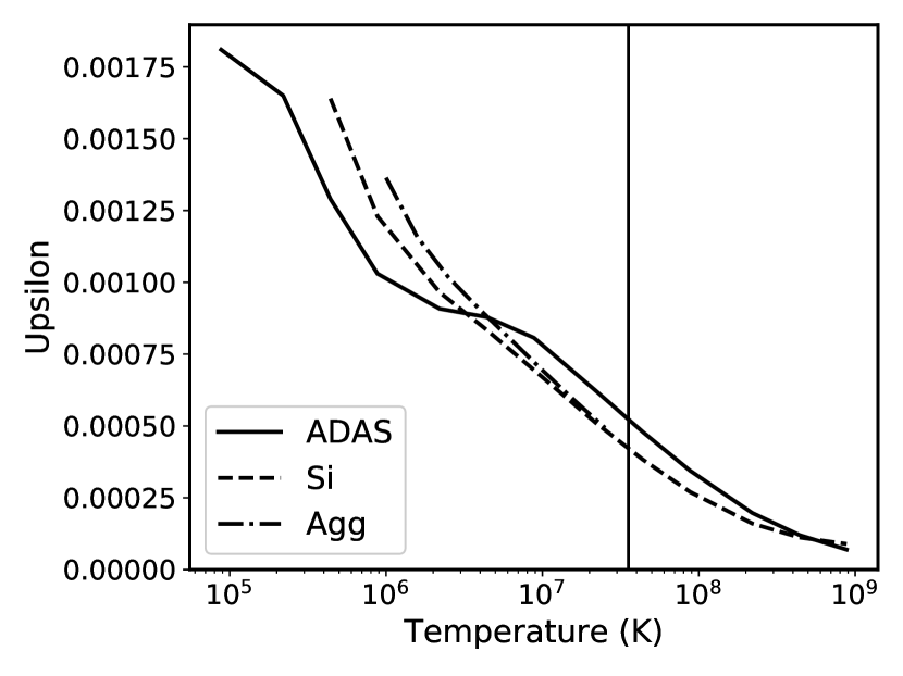
Figure 1: The effective collision strengths for the 1s^{2 1}S₀ to the 1s2s ³S₁ transition in Ti xxi. The vertical line is where the contribution function, or emissivity, for the radiative transition from the upper levels is maximum. ADAS refers to Whiteford et al. (2001), Si refers to Si et al. (2017) and Agg refers to Aggarwal & Keenan (2012)

2.4 Diagnostic ratios involving the Fe XXV satellites

As noted, the helium-like J satellites to the hydrogen-like Ly$\alpha$ lines have been observed and the ratio of the two provide a temperature diagnostic for high temperature plasmas. The J satellites are a collection of lines at somewhat longer wavelengths than the Ly$\alpha$ lines. Parmar et al. (1981) used the calculations of Dubau et al. (1981) for the analysis of their data. More recently, the observations of Pike et al. (1996) were analyzed with the updated calculations of Dubau et al. (1981). The new atomic data in CHIANTI allows one to calculate this ratio and the ratio is shown in Fig. 2. This consists of the ratio of the Fe xxvi 1s ²S_1/2 - 2p ²P_3/2 transition at 1.7780 Å to the Fe xxv 1s2p ¹P₁ - 2p^{2 1}D₂ transition at 1.7920 Å(the J satellite) and 17 other satellites at closely neighboring wavelengths. The ratio is comparable to that shown in Pike et al. (1996), although they use the sum of the Fe xxv satellite lines for values of n up to 20. Their ratio goes to a value of about 5 at 5 $\times$ 10⁷ K while our ratio goes to a value of about 2.7 at the same temperature.

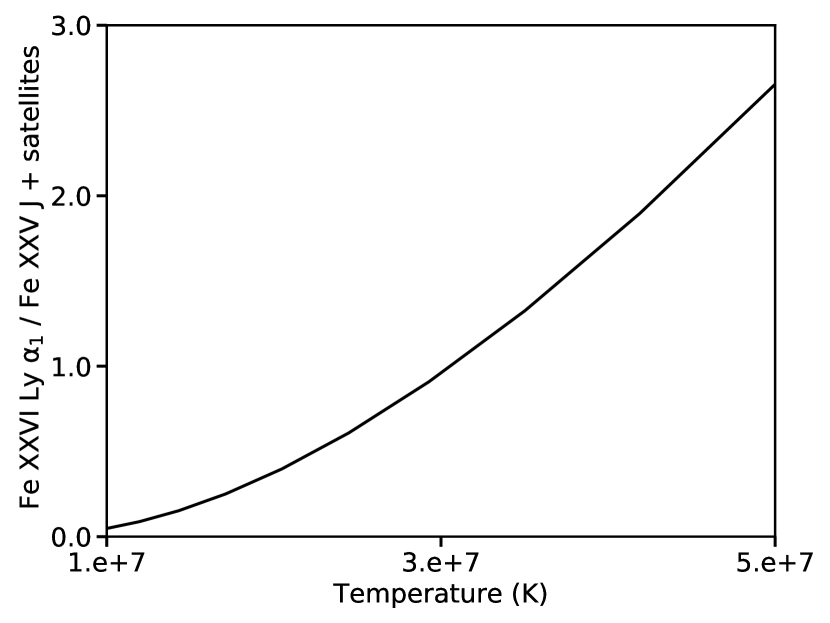
Figure 2: The ratio of the Fe XXVI Ly $\alpha_{1}$ line to the Fe XXV J satellite and the 17 strongest nearby Fe XXV satellite lines.

3 New atomic data for the beryllium isoelectronic sequence

It is well-known (cf. the review by Del Zanna & Mason, 2018) that spectral lines from Be-like ions are prominent and provide important density and temperature diagnostics. Of all the isoelectronic sequences, this was the one where the CHIANTI atomic data needed most improvements. In fact, for several Be-like ions, previous CHIANTI versions had either interpolated collisional rates (Keenan et al., 1986), or had sufficiently accurate data only for the $n=2$ (and sometimes $n=3$) levels. As previously shown in Del Zanna et al. (2008) for an important ion for the solar corona, Mg ix, interpolation of the rates can lead to incorrect results such as temperatures (with differences up to 50%).

As a baseline (unless otherwise stated), we have adopted for the ions in the sequence the CE rates calculated by Fernández-Menchero et al. (2014a) with the Breit-Pauli $R$-matrix suite of codes and the ICFT method. The CI and CC expansions included atomic states up to $nl=7{\rm d}$, for a total of $238$ fine-structure levels. Good agreement with the previous $R$-matrix CE rates for Mg ix (Del Zanna et al., 2008) and Fe xxiii (Chidichimo et al., 2005) were found by Fernández-Menchero et al. (2014a), but significant differences with other calculations are present. The $n=6,7$ levels only included $l=s,p,d$ states, which were added to improve the rates for the lower levels. The configuration expansion for the highest levels is typically unbalanced as energetically higher bound and continuum states are missing. Hence the A-values and the CE rates for some states can diverge substantially from the expected variation with the principal quantum number (see the discussion in Del Zanna et al. 2020). This is the case for the $n=6,7$ states. Therefore, only the 166 bound levels up to $n=5$ have been retained (reordering the indexing of the original calculation), unless otherwise stated.

For some ions, the levels above the ionization threshold have not been included, as proper treatment would require an extended two-ion model, including autoionisation rates. Only transition probabilities with a branching ratio greater than 10^-5 have been retained.

For the radiative data, we have replaced the values for the lowest configurations with data that are generally more accurate, checking that deviations for the strongest transitions were within 10-30%. For C iii and O v we adopted for the lowest 20 levels the A-values from the MCHF calculations by Tachiev & Froese Fischer (1999). Duplicates in the MCHF data were removed, and multipolar transition probabilities added. For the ions from Ne to Zn we adopted for the lowest $n=2,3$ states the A-values from the calculations of Wang et al. (2015), finding small differences (10% or so) with the APAP data. The latter used a combined Configuration Interaction and Many-body Perturbation Theory Approach (MBPT).

Comparisons with the earlier datasets show significant changes (20–30%) in the line intensities for many ions, even for the strong transitions. Experimental energies are taken from the NIST database, except where noted below.

3.1 C iii

C iii is a particularly important ion as it produces strong spectral lines. Only the lowest 75 bound levels up to $n=5$ were retained. Significant differences are present in the density- and temperature-sensitive ratio of the 2s 2p ¹P-2p^{2 1}S 1247.4 Å line with the lines of the 1176 Å multiplet (2s 2p ³P-2p^{2 3}P), when compared to the previous model, which included only the $n=2,3$ levels.

3.2 N iv

N iv has been the subject of extensive studies on the collisional rates. Aggarwal et al. (2016) performed relativistic electron scattering calculations for this ion with the DARC code, finding significant discrepancies with the ICFT results of Fernández-Menchero et al. (2014a), questioning the validity of the ICFT method. Previous doubts from the same authors were published (Aggarwal & Keenan, 2015), leading to a discussion on the importance of the target structure description by Fernández-Menchero et al. (2015a).

Fernández-Menchero et al. (2017) performed a large-scale electron impact excitation calculation for N iv using the B-spline R-matrix method, and compared the results with the ICFT and the DARC ones. The paper highlighted the importance of the target structure description and especially the size of the close-coupling expansion, pointing out that collisional rates to highly excited levels can be inaccurate, because of the limitation in the expansion.

The three sets of atomic rates obtained with the different methods provided an opportunity to obtain some estimates on the uncertainties, as well as their effect on the calculated emissivities of the lines. Del Zanna et al. (2019) showed that for astrophysical applications the three sets of data are equivalent, as very small (typically 10%) variations in the emissivities of the stronger lines were found.

For the present model we adopt the results of the B-spline method, as this was the largest-scale calculation, providing much better target energies than the other methods. Only the lowest 136 bound levels have been retained. Experimental energies from NIST as assessed by Fernández-Menchero et al. (2017) have been included.

3.3 O v

O v is another important ion, producing strong spectral lines widely used in solar physics. It is worth noting that the new model provides electron densities from within the lines in the 760 Å multiplet that are about 60% higher than the previous model. These lines have been resolved with e.g. the Solar and Heliospheric Observatory (SoHO) Solar Ultraviolet Measurements of Emitted Radiation (SUMER, see Wilhelm et al. 1995), and are now observed with the Solar Orbiter Spectral Imaging of the Coronal Environment (SPICE) spectrometer (Anderson et al., 2019).

The previous CHIANTI model was quite large, as it included a full set of configurations up to $n=5$. However, the collisional rates for most levels were calculated with the distorted wave method, except for the lower levels for which the results of an unpublished $R$-matrix calculation were used.

Experimental energies are taken from NIST. Only a few differences with the values in the previous CHIANTI version are present. However, we caution that several NIST energy values are not relative to the ground state, so the corresponding wavelengths might not be accurate.

3.4 Ne vii

The previous CHIANTI model for Ne vii had 46 $n=2,3$ levels, and $R$-matrix collisional rates. We note that some of the NIST experimental energies are not relative to the ground state so are uncertain.

3.5 Na viii, Al x, P xii, Cl xiv, K xvi, Ti xix, Cr xxi, Mn xxii, Co xxiv, and Zn xxvii

The previous CHIANTI models for Na viii, Al x, P xii, Cl xiv, K xvi, Ti xix, Cr xxi, Mn xxii, Co xxiv, and Zn xxvii had only the 10 lowest $n=2$ levels. Collisional rates were either interpolated along the sequence or were calculated with the DW codes (Ti xix, Cr xxi, Mn xxii, Co xxiv, and Zn xxvii). The present models are therefore a significant improvement over the previous ones.

For Al x, experimental energies for most levels have been taken from Khardi et al. (1994) as the NIST compilation is not complete. For Ti xix, Ti xix, Mn xxii, and Co xxiv we note that several NIST energies seem uncertain, and some are estimated values, i.e. not measured relative to the ground state.

3.6 Mg ix

Mg ix is an important ion for the solar corona, as it provides excellent temperature diagnostics (available with the Solar Orbiter SPICE spectrometer), see e.g. Del Zanna et al. (2008) and references therein. The previous CHIANTI model ion had 108 levels, with $R$-matrix collisional rates for the lowest 98 up to $n=4$, and a few $n=5$ levels with DW rates. The collision rates are close to the previous ones, so minor differences with the previous model are present. Experimental energies are taken from the previous CHIANTI version and from NIST.

3.7 Si xi

The previous model had $R$-matrix collisional rates calculated with a small target, only the 10 lowest $n=2$ levels, and only at intermediate energies. The rest of the CHIANTI model contained DW collisional rates.

Experimental energies have been re-assessed as both the previous CHIANTI version and the NIST values are surprisingly not complete. The values recommended by the extensive compilation of Kramida & Träbert (1995) have been adopted. These authors also provided $LSJ$ percentage composition which was key to identify many of the strongly spin-orbit mixed levels, where level assignment becomes difficult. They also provided uncertainty estimates for the observed energies. Their values are significantly different in many cases from those in NIST and in the previous CHIANTI version, but are generally very close to the theoretical energies of the new model. In a few cases, tentative energies have been assigned as observed, while in a couple of cases the Kramida & Träbert (1995) values could not be assigned to a level.

The new model for Si xi is a significant improvement for this important ion. Long-standing problems between predicted and observed intensities for this ion have been present for solar active regions. The strongest lines were observed by the SoHO CDS instrument. To illustrate the difference with the previous model, we have considered a CDS full-spectral atlas of an active region obtained on 1997 September 25 between 18:01 and 18:56 UT (s9253r00). This observation was one of those considered for the CDS in-flight calibration (Del Zanna, 1999; Del Zanna et al., 2001). A spatial area where the Si xi lines were enhanced was selected. The unblended lines were selected and the comparisons between observed and theoretical intensities, as a function of electron density and temperature, are presented in Figures 3,4 in the form of ‘emissivity ratios’ (see Del Zanna et al., 2004; Del Zanna & Mason, 2018, for details and examples), which are the ratios of the observed radiances $I_{\rm ob}$ of the lines with their emissivities, as a function of the electron density $N_{\rm e}$ (or temperature $T_{\rm e})$) for a fixed temperature (or density):

$$R_{ji}={I_{\rm ob}N_{\rm e}\lambda_{ji}\over N_{j}(N_{\rm e},T_{\rm e})\;A_{ji}}\;Const\;,$$ (1)

where $N_{j}(N_{\rm e},T_{\rm e})$ is the population of the upper level $j$ relative to the total number density of the ion, $\lambda_{ji}$ is the wavelength of the transition, $A_{ji}$ is the spontaneous radiative transition probability, and $Const$ is a scaling constant that is the same for all the lines within one observation. The value of $Const$ is chosen so that the emissivity ratios $R_{ji}$ are near unity where they intersect, so the scatter of the curves around unity provides a direct measure on the relative agreement between predicted and observed intensities.

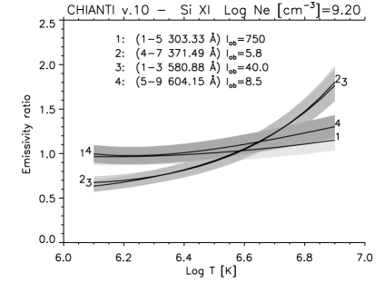
Figure 3: Emissivity ratios of the main Si xi lines observed by SoHO CDS in an active region, with the present v.10 model (above) and the previous one (v.9, below), as a function of the electron temperature. The labels indicate in parentheses the CHIANTI level indices of the lower and upper state, and the wavelength in Å. I_ob indicates the observed radiances in photon units. The shaded areas indicate the approximate uncertainty in the radiometric calibration.

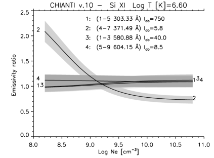
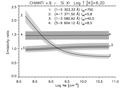
Figure 4: Emissivity ratios of the same lines as in Fig. 3, as a function of the electron density, with the present model (v10, above), and the previous one (v.9, below).

The 371.5 Å line is very weak but is strongly density-dependent. It indicates an electron density about $\times$10^9.2 cm^-3, with both the previous and current model. This density is typical of active region cores. The 604.1 Å line is also very weak. However, with the present model its intensity agrees with that of the other lines. With the previous version 9 model there is a discrepancy of 50%. The two main lines are the resonance line at 303.3 Å, observed in second order, and the intercombination line at 580.9 Å. They are an excellent temperature diagnostic for active regions (Del Zanna & Mason, 2018). With the current model, they indicate log $T$[K]=6.6, which is a reasonable value for an active region (4 MK). With the previous model, they provide a much lower temperature: log $T$[K]=6.2, i.e. 1.6 MK.

3.8 S xiii

S xiii is an important ion to measure the sulfur abundance in solar active regions. The previous model ion had many levels (92), but CE rates for the $n=2$ levels were interpolated along the sequence, and the other ones were calculated with the DW approach. Experimental energies are taken from NIST for the lowest levels, but for the rest energies have been re-assessed, mostly taking the values recommended by Fawcett & Hayes (1987).

3.9 Ar xv

The previous model ion was extended (92 levels), but CE rates for the $n=2$ states were interpolated along the sequence, and the other ones were calculated with the DW approach. Experimental energies are taken from NIST, but we note that many of the $n=3$ values were actually estimated with quantum defects by Khardi et al. (1994), so the wavelengths of the decays to the lower levels are not necessarily accurate.

3.10 Ca xvii

The previous model ion for Ca xvii was relatively accurate, given the importance of this ion, which produces strong EUV lines. It had 92 levels, with CE rates for the $n=2$ levels calculated with the $R$-matrix codes, and DW data for the rest of transitions. Experimental energies are taken from the previous CHIANTI version.

3.11 Fe xxiii

Fe xxiii is an important ion to study solar flares. The previous Fe xxiii model had $R$-matrix CE rates for the levels up to $n=4$, and DW rates for several $n=5$ levels. In addition, the model had autoionizing levels. We note that the previous CHIANTI v.9 model had observed energies from NIST. However, as several energies are far from the theoretical values, the CHIANTI v.8 experimental energies have been reinstated, with few additional energies taken from NIST. The data related to the autoionizing levels (producing the satellite lines) are the same as in version 9.

3.12 Ni xxv

The previous model for Ni xxv was relatively accurate, as it had $R$-matrix collisional rates for the lower levels, and DW rates for 92 levels up to $n=5$. Experimental energies are mostly taken from the compilation in the previous CHIANTI version, as it takes into account accurate measurements not included in the NIST compilation. We note that many differences are present between the NIST and CHIANTI energies.

4 New atomic data for the carbon isoelectronic sequence

The CE rates for all the ions in the C-like sequence (from from N ii to Kr xxxi), have recently been calculated by Mao et al. (2020) within the UK APAP network with the Breit-Pauli $R$-matrix suite of codes and the intermediate coupling frame transformation (ICFT) method. They included in the configuration interaction (CI) target and close-coupling (CC) collision expansion 590 fine-structure levels, arising from 24 configurations with $n\leq 4$ and the three configurations $2s^{2}2p5l$ with $l$=0–2.

The levels above the ionization threshold have not been included for some of the ions (as described below), as proper treatment would require an extended two-ion model, which is left for future updates. The A-values of the transitions among the ground configuration 2s² 2p² and the first excited 2s 2p³ levels have been taken from the MCHF calculations of Tachiev & Froese Fischer (2001) and the associated Tachiev (2004) as available online. Duplicates in the data were removed, and multipolar transition probabilities added.

Complete large-scale calculations of electron-impact excitation with the $R$-matrix codes for C-like ions were available in the previous CHIANTI version only for a few ions: Ne, S, and Fe. For most of the ions, $R$-matrix data were only available for the ground configuration $2s^{2}2p^{2}$ levels, with DW CE rates available for the excited configurations.

Ions from the C-like sequence provide widely-used density diagnostics (see, e.g. the review by Del Zanna & Mason, 2018) thanks to the metastability of the ground configuration levels. When benchmarking the new atomic rates, we found for many ions only relatively minor changes (about 20%) in the intensities of the strongest transitions. One exception is Ar xiii, because of an increase of about a factor of two in the CE rates for the forbidden transitions within the ground configuration, as shown in Mao et al. (2020). This affects the density diagnostics.

The reason why for most other C-like ions changes are not large is related to the fact that the populations of the ground configuration levels are strongly affected not only by the CE rates within them, but also by cascading from higher levels. In turn, the higher levels are mainly populated by direct impact excitation from the ground state via dipole-allowed transitions. As is well-known (but also shown in Mao et al. 2020) that the DW CE rates are often close to the $R$-matrix ones for the strongest allowed transitions, the result is that the populations of the ground configuration levels with the new models are not very different, despite some differences being present between the new and previous $R$-matrix CE rates within the ground configuration.

For N ii we have maintained the previous CHIANTI model as the CE rates are deemed more accurate.

4.1 O iii

For O iii we have retained the 177 bound levels of the Mao et al. (2020) calculations. Regarding the CE rates, as pointed out by Mao et al. (2020) and Morisset et al. (2020), those obtained with the ICFT calculations for the transitions among the ground configuration states differ from the more accurate values such as those calculated by Storey et al. (2014) and Tayal & Zatsarinny (2017) at the low temperatures typical of photoionized plasma. Tayal & Zatsarinny (2017) carried out a B-spline $R$-matrix calculation, but did not provide rates at sufficiently high temperatures needed for, e.g., solar plasma. Storey et al. (2014) performed a set of extended Breit-Pauli $R$-matrix calculations for transitions within the ground configuration, but only provided rates up to 25000 K. We have adopted these latter rates, and used the Mao et al. (2020) ones for the higher temperatures. In this way, we obtain accurate emissivities for the forbidden lines mostly used to study photoionized plasma and for the EUV lines mostly used in solar physics. For some transitions, the Mao et al. (2020) values at 25000 K are only 5–10% higher than the Storey et al. (2014) rates, this difference being comparable with the typical uncertainty of these calculations, as discussed by Storey et al. (2014). For the observed energies we used the NIST values, but note that several are uncertain, as they were not measured relative to the ground state. The previous CHIANTI model had 46 levels, and a mixture of $R$-matrix and DW data for the CE rates.

4.2 Ne v – Ca xv

For Ne v, the new model replaces one with 49 levels and $R$-matrix CE rates. We have retained 304 bound levels. In this case, nearly all the NIST experimental energies are in good agreement with the theoretical ones.

The new model for Na vi is a significant improvement, as it replaces one with only 20 levels and DW CE rates (except for the ground configuration). We have retained 410 bound levels.

The previous model for Mg vii had a mixture of scaled $R$-matrix data for the ground configuration, and DW rates for a total of 46 states. We have retained 450 bound levels.

For Al viii, the present model is a significant improvement over the previous one, which only had 20 levels and DW CE rates. We have retained 482 bound levels. Several NIST energies were uncertain and were not included. A few experimental energies for the ground configuration were improved.

The previous model for Si ix had 46 levels, and a mixture of $R$-matrix data for the ground configuration, and DW rates for the other states. We have retained all 590 levels.

The new model for P x is a significant improvement, as the previous model had only 20 levels and DW CE rates. Several NIST energies are uncertain.

The previous model for S xi was relatively extended, with 74 levels, and a a mixture of $R$-matrix data for the ground configuration, and DW rates for the other states. For several levels we have improved the experimental energies over the NIST values.

The new model for Cl xii is a significant improvement, as the previous model had only 20 levels and DW CE rates.

For Ar xiii, the new model produces line emissivities significantly different than the previous one, which was limited, as it had only 15 levels and DW CE rates. A comparison with version 9 for some important lines was shown in Mao et al. (2020). Experimental energies are from NIST, but we note that in many instances they are only approximate.

The new model for K xiv is also a significant improvement over the previous one, which had 20 levels and DW CE rates.

For Ca xv, we have retained all 590 levels, and used the MCHF ab-initio A-values calculated by G. Tachiev (2004) for the transitions among the ground configuration 2s² 2p² and the first excited 2s 2p³ levels. For these 15 states, the previous CHIANTI model had $R$-matrix CE rates, while for the remaining 31 levels only DW data were available.

4.3 Ti xvii – Zn xxv

The new models for Ti xvii, Cr xix, Mn xx, Co xxii, Ni xxiii, Zn xxv are a significant improvement over the previous ones, which had 20 levels and DW CE rates. The few available experimental energies are from NIST, with the exception of Zn xxv, for which we adopted the recommended values for the lowest 20 states by Edlen, and one level of Ni xxiii.

We note that Ekman et al. (2014) calculated accurate energies and A-values with GRASP2K for the C-like ions from Ar xiii to Zn xxv. If users are interested in identifying new experimental energies, the GRASP2K values should be considered. We have not included the A-values from Ekman et al. (2014) as they only provided E1 transitions, and also because the AS energies for these highly charged ions are close to the experimental ones and the A-values are relatively accurate.

4.4 Fe xxi

Fe xxi is an important ion in the sequence, given the large abundance of iron. Fe xxi lines are widely used in solar physics. The previous CHIANTI model had an extended set of CE rates calculated with the $R$-matrix codes by Badnell & Griffin (2001). As shown by Fernández-Menchero et al. (2016), that calculation was somewhat limited in the close-coupling expansion. The Fernández-Menchero et al. (2016) calculations included the same set of configurations in the CI expansion as in Mao et al. (2020), but differed in some details. A few issues were found by Mao et al. (2020) in the Fernández-Menchero et al. (2016) data, so we have replaced the previous model for the bound levels with the CE from Mao et al.

We have retained the experimental energies as in version 9. We have kept the Mao et al. A-values, as theoretical energies are quite close to the experimental ones. Very little differences with the previous set of A-values is present. Very small differences of a few percent are found for most of the strongest transitions, between the previous and the new model. The data for the autoionizing levels are the same as in the previous version.

5 New atomic data for the Mg isoelectronic sequence

Spectral lines from the Mg-like sequence are useful for a wide range of diagnostics (see, e.g. the review by Del Zanna & Mason, 2018). Among the most important ions in the sequence for solar physics are Fe xv and Si iii. For a discussion on Si iii see Del Zanna et al. (2015).

For this sequence, we have adopted the collisional rates calculated by Fernández-Menchero et al. (2014b) with the ICFT $R$-matrix codes for all the ions from $\mathrm{Al}^{+}$ to $\mathrm{Zn}^{18+}$. The target includes a total of 283 fine-structure levels in both the CI target and CC collision expansions, from the configurations $1\mathrm{s}^{2}\,2\mathrm{s^{2}p^{6}}\,3\{\mathrm{s,p,d}\}\,nl$ with $n=4,5$, and $l=0-4$. For some ions listed below, levels above the ionization threshold have not been included, as proper treatment would require an extended two-ion model, which is left for future updates.

As in the case of the Be-like sequence, previous CHIANTI versions did not have atomic rates for many minor ions, and for the less important ones only had a very limited set of levels and DW CE rates. As shown in Fernández-Menchero et al. (2014b), significant differences with the DW rates are present.

For the radiative rates, we have mostly used the values from the MCHF calculations by Tachiev & Froese Fischer (2002) for the lowest 26 $n=3$ levels ($3s^{2},3s3p,3p^{2},3s3d,3p3d$). Duplicates in the data were removed, and multipolar transition probabilities added. Differences with the Fernández-Menchero et al. (2014b) values were typically at most 20-30%. Experimental energies are taken from NIST unless stated otherwise.

5.1 Al ii

The previous CHIANTI model had 20 levels and CE rates obtained from various sources. We have retained the lowest 60 bound states of the Fernández-Menchero et al. model. Experimental energies are taken from NIST, but we note that a few are uncertain. The original radiative data in Fernández-Menchero et al. (2014b) have been retained for consistency, as significant differences with the MCHF calculations for the higher levels are present.

5.2 Si iii

The previous CHIANTI model had 20 levels and $R$-matrix CE rates. We have retained the lowest 82 bound states of the Fernández-Menchero et al. model. Experimental energies are taken from Del Zanna et al. (2015) and NIST.

5.3 P iv, Cl vi, K viii, Mn xiv, Co xvi, and Zn xix

P iv, Cl vi, K viii, Mn xiv, Co xvi, and Zn xix are new additions to the database. For P iv, Cl vi, K viii we have retained, respectively, the lowest 117, 171, 209 bound states of the Fernández-Menchero et al. model.

5.4 S v, Ar vii, Ti xi, and Cr xiii

The previous CHIANTI models for S v, Ar vii, Ti xi, and Cr xiii were very limited, as they had only 16 levels. S v, Ar vii, Cr xiii had DW CE rates calculated in $LS$ coupling. Ti xi had interpolated CE rates. For S v, Ar vii we have retained the lowest 159, 196 bound states of the Fernández-Menchero et al. model. Significant differences with the previous CE rates are present, as shown for S v by Fernández-Menchero et al.

5.5 Ca ix

The previous CHIANTI model contained complete set of 283 levels up to $n=5$, but DW CE rates. Autoionising levels were also present. We have retained the lowest 220 bound states of the Fernández-Menchero et al. model. Experimental energies are taken from the previous CHIANTI version.

5.6 Fe xv

The previous CHIANTI model was extended, with the complete set of 283 levels up to $n=5$, and $R$-matrix CE rates for the $n=3$ levels, and DW CE rates for the higher levels. The experimental energies of the previous version 9 are retained. As mentioned in Fernández-Menchero et al. (2014b), significant differences with the previous $R$-matrix CE rates are present in some cases, for this important ion. As a follow-up, Fernández-Menchero et al. (2015b) discussed in more detail some Fe xv transitions, and presented a benchmark against solar data.

5.7 Ni xvii

The previous CHIANTI model was relatively extended, with the complete set of 159 levels up to $n=5$, but DW CE rates. Observed energies are taken from a variety of sources, as detailed in the database.

6 Other updated ions

6.1 Fe xii

Experimental energies of a few $n=3$ levels in Fe xii were changed in version 9 following the work of Wang et al. (2018a), which confirmed most of the identifications by Del Zanna & Mason (2005). However, by mistake the indexing of two levels (37,38) was interchanged, so the energies for these two levels were incorrect. This has been fixed. The energies of a few $4d$ levels have now been changed, following Song et al. (2020). These authors have carried out MCDHF calculations and compared predicted and observed wavelengths for the $n=4$ levels. Excellent agreement with the wavelengths of the new identifications proposed by Del Zanna (2012) was found. Generally, excellent agreement was also found with the wavelengths and identifications by Fawcett et al. (1972), with the exception of several $4d$ levels. After checking the original plates used by Fawcett et al. (1972), and estimating line intensities based on the Del Zanna et al. (2012a) calculations, Song et al. (2020) recommended a few new values, which have been adopted here.

6.2 Fe xi

Wang et al. (2018b) carried out extensive MCDHF calculations for the $n=3$ levels in Fe xi, and compared energies with literature values. For the $3s^{2}3p^{3}3d$ levels, producing the strongest lines, they found excellent agreement (within a few hundreds of Kaysers) with all the new identifications proposed by Del Zanna (2010) and included in previous CHIANTI versions. For the $3s3p^{3}3d$ levels, the four previous tentative identifications proposed by Del Zanna (2010) have been revised following Wang et al. (2018b).

6.3 Fe x

Wang et al. (2020) carried out extensive MCDHF calculations for Fe x, and assessed the wavelengths and identifications, as present in NIST, the previous CHIANTI versions, and literature values. Good general agreement with the values proposed by Del Zanna et al. (2004) and Del Zanna et al. (2012b), included in previous CHIANTI versions was found, with notable discrepancies in a few NIST energies. On the basis of the Wang et al. (2020) assessment, we have introduced 8 revised experimental energies, three from Jupen et al. (1993), one from Del Zanna et al. (2012b) and four from NIST.

The energy separation of the ⁴D_7/2 and ⁴D_5/2 has been modified by using the recent measurement by Landi et al. (2020), decreasing it from the previous 5.5 cm^-1 value (see the discussion in Del Zanna et al. 2004) to 2.29 cm^-1. This change has negligible effects on the wavelengths of the lines emitted by these levels around 257.26 Å, but it has a critical importance for the measurement of magnetic field strength using the magnetically induced transition from the ⁴D_7/2 level to the ground (Landi et al. 2020b, in press).

6.4 Ni xii

Regarding Ni xii, we base our new model on the Breit-Pauli $R$-matrix calculations carried out with the ICFT method by Del Zanna & Badnell (2016). The CI expansion included the complete set of atomic states up to $n=4$, but for the CC expansions in the scattering calculation only the lowest 312 $LS$ terms were retained. This is a significant improvement over the previous calculations (available in the previous CHIANTI version) which included only the lowest 14 terms (up to 3d), producing 31 fine-structure levels. We provide only the lowest 589 fine-structure levels, as the higher ones are not reliable. A key feature of the Del Zanna & Badnell (2016) calculations is the inclusion of semi-empirical corrections in the structure and scattering calculations. This provides a significant improvement in the rates.

Very few energy levels were known for this ion, the most important ones only relative to the 3d ⁴D_7/2 (the same situation which occurred in Fe x, resolved by Del Zanna et al. 2004). Del Zanna & Badnell (2016) provided a discussion of the various optional line identifications, and suggested several new ones. The MCDHF calculations by Wang et al. (2020) were used by the same authors to confirm some of those identifications and suggest new ones. We adopt these latest values in the present model, but point out that further laboratory studies are needed to confirm these identifications.

6.5 Cr VIII

Cr viii was added to CHIANTI in version 6 (Dere et al., 2009) using data from an unpublished calculation of E. Landi. This has been replaced with the data from Aggarwal et al. (2009) giving a model with 362 fine structure levels from 10 configurations.

Experimental energies are only available for 21 levels and have been taken from the NIST database. Aggarwal et al. (2009) performed a number of structure calculations, and the theoretical energies used for CHIANTI are those from the GRASP calculation with Breit and QED corrections. Radiative data are also from the GRASP calculation. This data-set was filtered such that, for each atomic level, only those decay rates that were $>10^{-5}$ of the maximum decay rate from that level were retained.

Upsilons were calculated by Aggarwal et al. (2009) using the Flexible Atomic Code and were tabulated at nine temperatures from $\log\,T=5.0$ to 6.6 at 0.2 dex intervals. Cr viii has 10 metastable levels plus the ground state and only those transitions from these 110 levels were included in the CHIANTI data file. The collision dataset was assessed following the procedure described in CHIANTI Technical Report No. 4 and 69 allowed transitions were found not to tend towards their high temperature limits, with the limits generally higher than the upsilon values sometimes by as much as a factor 100. These discrepancies may stem from the different structure models used for the radiative and collisional calculations. For these 69 transitions, the high temperature limits were removed from the fits. The final CHIANTI scaled-upsilon file reproduces the original upsilon data to better than 0.2%.

6.6 Fe VII

Fe vii has not been updated since CHIANTI 5 (Landi et al., 2006), and the model contained only the nine levels of the ground configuration. The new model has 189 fine-structure levels of the $3p^{6}3d^{2}$, $3p^{5}3d^{3}$, $3p^{5}3d4l$ ($l=s,p,d,f$) and $3p^{5}3d5l$ ($l=s,p$) configurations. The model was not previously updated because inconsistencies between line intensities calculated with the Witthoeft & Badnell (2008) model and solar observations (using the NIST identifications) were noted, but different explanations were given: Young & Landi (2009) revised some NIST identifications but assumed that the inconsistencies were due to problems in the atomic rates. Del Zanna (2009) provided an alternative set of identifications where agreement with observations was obtained, pointing out that the Witthoeft & Badnell (2008) model was relatively correct, by comparison with a large-scale benchmark calculation. Later, Tayal & Zatsarinny (2014) provided a new large-scale scattering calculation producing similar rates to those of Witthoeft & Badnell (2008).

The new model follows the assessment of Young et al. (2020, submitted), which relies on new laboratory measurements. Some inconsistencies are still present but the new model represent a significant improvement over the previous one. The experimental energies are mostly taken from the NIST database, but some new values are taken from Young et al. and Young & Landi (2009). Theoretical energies for 134 levels are taken from Li et al. (2018), while the remaining energies are from Tayal & Zatsarinny (2014). We note that the Li et al. (2018) energies show much better agreement with the experimental energies than those of Tayal & Zatsarinny (2014), and so they yield more accurate wavelengths for transitions involving levels without experimental energies.

Radiative decay rates for allowed transitions are from Tayal & Zatsarinny (2014). Forbidden transition data are from Li et al. (2018), supplemented with values from Witthoeft & Badnell (2008), where necessary.

Collisional excitation rates are from Tayal & Zatsarinny (2014). The CHIANTI assessment procedure identified a number of allowed transitions for which the rates did not tend towards the high temperature limit points, usually with the latter being too high. These cases likely arise because the decay rates were derived from a more elaborate structure calculation than used for the scattering calculation. They were treated by adjusting the upsilon scaling parameter to enable a smooth transition to the high temperature limit.

6.7 O II

It was brought to our attention that four A-values within the ground configuration of the N-like O ii were incorrectly assigned. We have now replaced them with the correct ones, noting that this error only affected the intensities of some of the forbidden lines within the ground configuration. We have also improved the experimental energies and associated wavelengths using literature values.

7 New additions to the database

7.1 Cr II

The vanadium-like ion Cr ii has been added to CHIANTI. Tayal & Zatsarinny (2020) provided radiative decay rates and Maxwellian-averaged collision strengths (upsilons) for 512 fine structure levels of the $3d^{5}$, $3d^{4}5s$, $3d^{4}4p$, $3d^{3}4s^{2}$ and $3d^{3}4s4p$ configurations. Experimental energies were available for 378 levels and were taken from the NIST database. We note that the agreement between the experimental energies and the Tayal & Zatsarinny (2020) calculated energies is excellent, with a mean discrepancy of 38 cm^-1. The radiative decay rate data-set was filtered such that, for each atomic level, only those decay rates that were $>10^{-5}$ of the maximum decay rate from that level were retained.

Based on the radiative data we determined that there are 117 metastable levels (including the ground) and so the upsilon data-set was filtered so that only those transitions for which the lower level was a metastable were included. Upsilons were tabulated for 20 temperatures between $10^{3}$ and $10^{5}$ K. The assessment method described in CHIANTI Technical Report No. 4 was applied to the data-set and no problem transitions were found. The scaled upsilon data stored in CHIANTI reproduce the original data to better than 0.5% for all transitions and temperatures.

8 Population lookup tables and other improvements

IDL software has been written to generate lookup tables for level populations for all ions in the database. The CHIANTI software can then use these tables to obtain level populations rather than compute them from the atomic data. This has significant time savings for the large ion models in CHIANTI. For example, a synthetic spectrum that would usually take about 10 minutes to compute can be obtained in less than a minute with the lookup tables.

To create the lookup tables, the software scales the level populations by one of two formulae, depending if the level is a metastable or not:

$$n_{i}^{\prime}=\left\{\begin{array}[]{cl}10^{5+\alpha_{i}/T}n_{i}&\quad{\rm[regular]}\\ 10^{20+\alpha_{i}/T}{n_{i}\over N_{\rm e}}&\quad{\rm[metastable]}\\ \end{array}\right.$$ (2)

where $T$ is temperature, $N_{\rm e}$ is the electron number density, $n_{i}$ the level population computed by the IDL routine pop_solver, and $\alpha_{i}$ a scaling parameter described below. The $n_{i}^{\prime}$ are computed for a temperature range $T_{0}$ to $T_{1}$ determined from the default ionization equilibrium file distributed with CHIANTI to be those temperatures for which the ionization fraction values are $\geq 10^{-8}$ of the peak value. The density range is set by the user. The temperature and density grids are set on a logarithmic scale with intervals of 0.05 and 0.2 dex, respectively.

The advantage of tabulating the level populations rather than, say, the emissivities or contribution functions is that the data-set is much smaller. For example, the density range $\log\,N_{\rm e}=7$ to 13 yields tables with a total size of about 0.5 Gbytes.

The temperature dependence of a level population is usually given by $\exp(-1/T)$, hence the temperature factor in Eq. 2. The parameter $\alpha$ is determined from the following expression:

$$\alpha={T_{0}T_{1}\over T_{1}-T_{0}}(\log\,\bar{n}(T_{1})-\log\,\bar{n}(T_{0}))$$ (3)

where $\bar{n}(T)$ is the mean value of the level population over the density range of the lookup table.

The scaling applied to the level populations is chosen to remove the dominant temperature and density dependent terms from the tabulated quantity. When deriving populations from the lookup tables bilinear interpolation is used, and the accuracy of the derived populations is typically better than 1%. Further details of the method are given in CHIANTI Technical Report No. 16.

A set of lookup tables is provided for Solarsoft users in the CHIANTI package, computed over the density range $\log\,N_{\rm e}=7$ to 13. For other users tables for all ions can be generated with the routine ch_lookup_all_ions.

A /lookup keyword has been added to key IDL routines such as dens_plotter, temp_plotter and ch_synthetic to implement the lookup tables. In addition the new routines ch_lookup_emiss and ch_lookup_gofnt yield emissivities and contribution functions from the lookup tables. A key feature of the software is that the CHIANTI version number is checked to ensure the lookup tables come from the latest version of the database.

Finally, we have also introduced other ways to speed-up the calculations. One is to store the CE rates as compressed FITS binary tables, which are faster to read than the ascii files (which are still kept in the database). We have also added the option to use the LAPACK version of the invert program when calculating the populations from the rate matrix.

9 Improved recombination rates and ionization equilibria

New calculations of the radiative and dielectronic recombination rates for silicon-like ions recombining to phosphorus-like ions have been presented by Kaur et al. (2018). These have been incorporated into CHIANTI together with a new calculation of the ionization equilibrium. They do not represent large changes in the ionization equilibrium. For the case of calcium, the changes between the Version 9 and the new Version 10 ionization can be seen in Fig. 5. The temperatures of maximum ionization equilibrium for Ca vi is 3.2 $\times$ 10⁵, for Ca vii is 4.5 $\times$ 10⁵ and for Ca viii is 5.6 $\times$ 10⁶ K for the new version dataset.

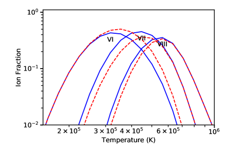
Figure 5: A comparison of the new ionization equilibrium (blue line) to that of version 9 (red dashed line) for several stages of calcium

10 Dielectronic recombination (DR)

10.1 Dielectronic recombination into helium-like ions

Recently, a large-scale collisional-radiative model for helium emission in the solar corona was developed (Del Zanna et al., 2020). Whilst benchmarking the various atomic rates, some inconsistencies in the current CHIANTI model for neutral helium were found. However, the present model has not been modified as it is very limited in terms of physical processes included. The main error that was found was in the dielectronic recombination (DR) into neutral helium, as calculated by N.R.Badnell. New DR rates were recalculated by Del Zanna et al. (2020). The new rates are about a factor of two higher and have now been included in CHIANTI. The error was also present (albeit not as large) for the corresponding Li, Be, and B ions, which have also been updated in the UK APAP repository and in the present CHIANTI version.

10.2 Suppression of dielectronic recombination rates

CHIANTI uses total DR rate coefficients in the calculation of the equilibrium ionization balance, and the so-called "zero-density" rates are used, meaning there is no density sensitivity. It is known, however, that DR rates become suppressed at high densities as the increased electron collision rates de-populate the high-lying levels that are important in the DR process. Summers (1974) modeled this process, and Nikolić et al. (2018) provided a fitting formula that is applicable to all ions in the CHIANTI database. With CHIANTI 10 we have coded the Nikolić et al. (2018) suppression factor formula and the IDL routine ch_dr_suppress returns the DR rate coefficient for any ion for a specified electron number density ($N_{\rm e}$) or electron pressure ($P$). If the latter is specified, then the density is set to $P/T$, where $T$ is the temperature.

A consequence of the DR rates is that the equilibrium ionization balance table (stored in a CHIANTI "ioneq" file) becomes density dependent. The IDL routine make_ioneq_all generates the ioneq file and it now takes the optional inputs "density" and "pressure". The default CHIANTI ioneq file that is distributed with the database (named "chianti.ioneq") continues to be the zero-density table.

We caution that the suppression factor formula is by itself an approximation to effective recombination coefficients obtained with a simplified treatment, and that there are other sources of density sensitivity to the ionization equilibrium equations that are not modeled. In particular that due to ionization/recombination out of metastable levels, as recently discussed for carbon and oxygen ions by Dufresne & Del Zanna (2019) and Dufresne et al. (2020).

Further details are given in CHIANTI Technical Report No. 17, and examples of the use of the new ioneq files are given in Young et al. (2018) and Young (2018).

11 Conclusions

As described in a recent review on the status of the atomic data and modelling available within CHIANTI (Del Zanna & Young, 2020), the present version is a significant step forward in terms of completeness of atomic data for astrophysical ions. Significant improvements are provided for several ions for which little or no data were available. The most important improvements are for the ions of the Be-like sequence, as we have shown with one example. For those cases where accurate atomic data were available in the previous version, the recent large-scale calculations (scattering and radiative) often produce line emissivities for the strongest lines that are reasonably close (within 10-20%) to those obtained from the previous data, providing confidence in the atomic data and also a measure on the overall uncertainties. As briefly mentioned here and also pointed out in Del Zanna & Young (2020), several improvements on the modelling side are however still required within the CHIANTI package. The inclusion of more physical processes such as photoionization, charge exchange, collisional ionization from excited states will be considered in future releases.

References

- Aggarwal et al. (2009) Aggarwal, K. M., Kato, T., Keenan, F. P., & Murakami, I. 2009, A&A, 506, 1501
- Aggarwal & Keenan (2012) Aggarwal, K. M., & Keenan, F. P. 2012, Phys. Scr, 85, 065301
- Aggarwal & Keenan (2015) —. 2015, MNRAS, 447, 3849
- Aggarwal et al. (2016) Aggarwal, K. M., Keenan, F. P., & Lawson, K. D. 2016, MNRAS, 461, 3997
- Anderson et al. (2019) Anderson, M., Appourchaux, T., Auchère, F., et al. 2019, A&A, doi:https://doi.org/10.1051/0004-6361/201935574
- Badnell (2011) Badnell, N. R. 2011, Computer Physics Communications, 182, 1528
- Badnell et al. (2016) Badnell, N. R., Del Zanna, G., Fernández-Menchero, L., et al. 2016, Journal of Physics B Atomic Molecular Physics, 49, 094001
- Badnell & Griffin (2001) Badnell, N. R., & Griffin, D. C. 2001, Journal of Physics B Atomic Molecular Physics, 34, 681