Image transmission through a dynamically perturbed multimode fiber by deep learning

Abstract

When multimode optical fibers are perturbed, the data that is transmitted through them is scrambled. This presents a major difficulty for many possible applications, such as multimode fiber based telecommunication and endoscopy. To overcome this challenge, a deep learning approach that generalizes over mechanical perturbations is presented. Using this approach, successful reconstruction of the input images from intensity-only measurements of speckle patterns at the output of a 1.5 meter-long randomly perturbed multimode fiber is demonstrated. The model’s success is explained by hidden correlations in the speckle of random fiber conformations.

Shachar Resisi, Sebastien M. Popoff, Yaron Bromberg*

Shachar Resisi, Yaron Bromberg
Racah Institute of Physics, The Hebrew University of Jerusalem, Jerusalem 91904, Israel
Email Address: yaron.bromberg@mail.huji.ac.il
Sebastien M. Popoff
Institut Langevin, CNRS, ESPCI Paris, Université PSL, 75005 Paris, France

1 Introduction

Multimode optical fibers (MMFs) hold great promise for increasing the capacity of data transmission, especially for applications such as optical communication systems [1], fiber lasers [2] and endoscopic imaging [3, 4, 5, 6, 7]. An important challenge such applications face is the inherent sensitivity of fibers to various types of fluctuations, such as thermal, acoustic, or mechanical perturbations. Unless special fibers are used [8], such perturbations dramatically change the transmission properties, since modal interference is extremely sensitive to changes in the phase accumulated by the fiber’s guided modes, which are in turn affected by the perturbations. Overcoming the effects of these perturbations is an important step towards robust fiber-based technologies and applications.

For one static conformation of the fiber, the transmission properties are fully captured by the transmission matrix (TM) [9]. When weak perturbations are applied on the fiber, the TM of the deformed fiber can be predicted [7, 10], mapped to pre-calibrated deformations [11], or compensated for [12, 13, 14]. Unfortunately, these options do not hold for strong deformations. Invariant statistical properties can also be harnessed to recover the transmitted information. For example, a rotational memory effect was observed in pixel space [15], and recently a similar effect in mode basis was used for image reconstruction through MMFs [16]. Alas, these properties are also limited to small perturbations and require a prior estimation of the TM or a feedback signal. The existence of invariant properties that survive strong deformations would allow envisioning image reconstruction through unknown and strongly perturbed fibers.

The high availability and low cost of strong computing power in recent years gave a significant boost to deep learning (DL) approaches. Recently, neural networks have attracted increasing attention in the optical community, allowing for the reconstruction of input information after propagation through random complex media [17, 18, 19, 20, 21, 22, 23, 24, 25, 26, 27, 28]. In fibers, convolutional neural networks (CNN) were shown to produce reconstructions with a similar fidelity to the TM approach [18, 19, 21]. Most previous works were limited to a single, static, fiber conformation. It was recently shown that CNN models can reconstruct images from fibers that are weakly perturbed while the data sets were recorded. The weak perturbations were induced by natural drifts in the environmental conditions [19], by weak bending of the fiber [21, 28] or by wavelength scanning [29]. Nonetheless, all previous works in fibers were not able to generalize to unknown and strongly perturbed fiber conformations that span a wide configuration space which describes numerous uncorrelated fiber configurations. DL approaches are known to efficiently learn invariant properties of signals, and can thus be harnessed for the challenge of learning the transmission through strongly perturbed systems. Indeed, in scattering media, Li et al. trained a CNN on the speckle created by a group of thin diffusers, and produced excellent image reconstructions from speckle resulting from different diffusers of the same type [20, 30]. This generalization was possible due to the existence of correlations between speckle created by the different diffusers, an invariant property which the DL model learned to recognize.

Motivated by these results, we use DL to learn invariant properties of strongly perturbed multimode fibers. We use a CNN and show that when we train the network over hundreds of random nearly uncorrelated fiber bends, it succeeds in reconstructing high-fidelity images even when the fiber is strongly perturbed many weeks after the training perturbations. We call this method of training on multiple low-correlated fiber conformations configuration training. A sketch of our workflow is presented as Figure 1. Configurations are created via strong mechanical perturbations, by simultaneously bending the fiber at multiple positions using an array of piezoelectric plate benders that are positioned above the fiber [31]. We suggest that the generalization is possible due to some hidden statistical similarities in the speckle, and support this by showing these correlations along with a 2-dimensional (2D) embedding of the acquired speckle.

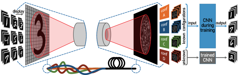
Figure 1: Schematics of the reconstruction process. Images from the MNIST hand-written digit dataset are displayed on a digital micromirror device (DMD). A laser beam is reflected from the DMD and injected on a multimode fiber, whose distal end is imaged on a CMOS camera. This procedure is repeated for each fiber conformation that we change by applying local bends at multiple positions along the fiber (depicted by the orange, blue, green and red curves). For the same set of input images (hand-written digits), different configurations give different output speckle patterns. Speckle-digit pairs from some of the configurations (coined the known configurations) are used to train a convolutional neural network (CNN). Speckle from unknown configurations are used to reconstruct digit input images and estimate the generalization capabilities of the trained model.

2 Methods

2.1 Experimental setup

The experimental setup, as depicted in Figure 2, consists of a HeNe CW laser (wavelength of $\lambda=632.8$ nm) which illuminates a digital micromirror device (DMD; Ajile AJD-4500-UT). The light from the DMD’s on pixels is imaged on the proximal end of a 1.5 meter-long step-index MMF (Thorlabs FG050LGA; V number $\approx 55$ at $\lambda$) using a $4f$ system. The intensity of the output speckle pattern is imaged by a second $4f$ system on a CMOS camera. We place 37 piezoelectric actuators along the fiber, and use a computer to control their vertical displacement. Each actuator bends the fiber by a three-point contact, creating a bell-shaped local deformation of the fiber, and inducing mode mixing exhibited in the fiber’s transmission matrix [32]. The curvature of the bend depends on the vertical travel of the actuator, and is on the scale of millimeters (down to $\sim 12$ mm; see Figure 2(b) and 2(c)) [31]. By changing the actuator’s position, and composing the bends created by all actuators, we can create a huge variety of possible configurations, with varying correlations between each other. To quantify the correlation between different random fiber conformations, we compute the Pearson correlation coefficient (PCC) between speckle patterns obtained for a fixed input. When we randomize the bending configuration created by all of the actuators using their full stroke, the average PCC between different fiber conformations (calculated over the same input patterns) is $0.12\pm 0.01$, which we find to be equivalent to the PCC values obtained by simply bending the fiber on centimeter scales (see supplementary material for more details). These similar correlation values in multiple bending regimes emphasize the system’s relevance for studying general bending deformations.

2.2 Data acquisition and processing

To collect many different speckle patterns for a single fiber geometry, we display sequences of hand-written digit patterns from the MNIST dataset [33] on the DMD and record the resulting $128\times 128$ speckle pattern. Due to the binary nature of the DMD, each digit is first converted to a binary amplitude image by applying a threshold on the original 8-bit grayscale image. The number of digit patterns and fiber configurations we acquire varies in the different training approaches we study. In all cases, we acquire separate data for training and for testing purposes (according to the division of the original dataset [33]).

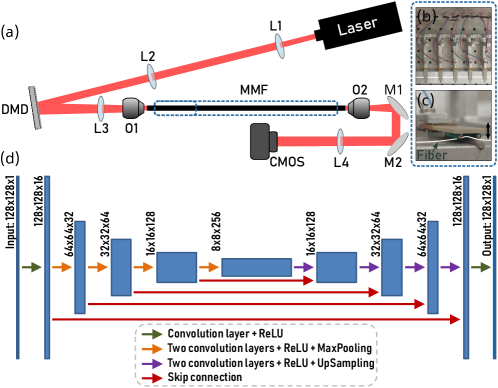
Figure 2: Experimental setup and neural network architecture. (a) A laser beam illuminates a DMD. The reflected light is imaged onto the proximal end of an MMF. Piezoelectric plate benders are positioned above the fiber (b), allowing for the application of various computer-controlled bends along the fiber. The light from the distal end of the fiber is imaged on a camera. (c) Side view of a bend, applied by a three-point contact between the actuator and an opposing metal rod. The curvature’s radius varies on the scale of $mm$-s. (d) Schematic of the U-Net architecture used for image reconstruction from speckle obtained at multiple fiber geometries. L, lens; DMD, digital micromirror device; O, objective; MMF, multimode fiber; M, mirror; CMOS, camera.

The deep learning model we use is a convolutional neural network (CNN) of U-Net type [34]. We feed the network with speckle images, and reconstruct the digit patterns that were displayed on the DMD. Once the training is complete, predictions are made in real time (milliseconds). The exact architecture we use is depicted in Figure 2(d) (see supplementary material for more details). The metrics we use to quantitatively appraise the performance of our model are the pixel-wise accuracy (defined as the percentage of the correctly predicted pixels) and the Jaccard index (JI; the intersection over union score of the binary reconstructions, which ranges between 0 to 1, and is only affected by the white pixels). Additionally, we train a very simple CNN [35] to classify the reconstructions into digits, and compare each result with the digit number that was displayed on the DMD. We define the classification success as the true positive rate and calculate it over unknown patterns to assess the generalization capabilities of the trained model.

3 Experimental Results

We start by demonstrating the reconstruction of a single configuration. For this first experiment we acquire a total of 70k different images (originating from 70k different hand-written digit patterns in the MNIST dataset), of which 60k are used for training and the rest 10k only for testing. We use the training set to train the model, and use the unknown test set to appraise its performance. As expected for an unperturbed fiber, and in accordance with previous works, the reconstruction is very accurate, see Figure 3. Quantitatively, the average pixel-wise accuracy for the entire test set (averaged over 10k reconstructions) is $97.6\%\pm 0.2$, the JI is $0.83\pm 0.02$, and the classification success is over 97%. While yielding high fidelity reconstructions for the same fiber conformations, this model fails to generalize over unknown fiber perturbations, resulting in an average pixel accuracy of $82.8\%\pm 3.2$ and JI of $0.17\pm 0.07$ as demonstrated in the bottom row of Figure 3(c).

In principal, one could extend this approach and train a CNN on all of the data from multiple configurations. In the supplementary material, we demonstrate this for simultaneously training on 8 random fiber conformations. However, since each actuator induces significant mixing between the fiber modes [32], the space representing the possible configurations induced by 37 actuators is very large, even for a short fiber. To statistically explore this space, a large number of configurations needs to be represented in the training set. The current approach, to which we refer as standard training, is not scalable for a large number of configurations, as it requires a large data set for each configuration and thus the training set becomes too large to be handled efficiently in terms of memory (needed to store the images) and time (to train the network).

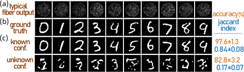
Figure 3: Digit reconstruction using a CNN trained on a single fiber conformation. (a) Example of speckle patterns received at the distal end of the fiber for a random configuration. (b) The ground truth, i.e. the image that is sent to the DMD. (c) The top row shows representative examples of reconstructions from a known configuration (the one the model was trained on). The bottom row shows examples of an unknown configuration, from which it is evident that the model does not generalize to other fiber conformations. The corresponding inputs were not used as part of the training process. The pixel-wise accuracy, calculated over the patterns in each row appears in orange, and the Jaccard index (JI) in blue.

As one cannot expect to learn all of the possible conformations of the fiber, predicting the output from an unknown configuration can be possible if there are invariant properties that are robust to conformation variations and are learned by the CNN. To harness these potential invariant properties, we train the network over 943 fiber conformations, obtained by randomizing the positions of all of the actuators. The degree of correlation between fiber conformations, quantified by the PCC of speckle patterns obtained for the same fiber input, is $0.12\pm 0.01$. To account for the large number of configurations while limiting the size of the training set, we use only 800 training images per configuration and record the intensity of the resulting speckle. In total, data was acquired over the span of 14 weeks, during which a few different macro bends were applied in addition to the actuator-induced bends to improve the model’s robustness to mechanical perturbations of varying scale. The same average PCC was obtained between configurations from the same and different days, regardless of the applied macro bend. We acquire additional test data from 800 other random fiber conformations, to appraise the performance of the model on unknown configurations. We coin this type of training, which consists of less data from multiple fiber conformations as configuration training, because we prompt the model to learn general statistically invariant properties.

The configuration training immensely improves the reconstruction of test images from unknown fiber conformations. We observe that when the average correlation between configurations from the train set and the test set (calculated for the same input patterns) is 0.12, the average Jaccard index increases from $JI=0.13$ for standard training to $JI=0.47$ for configuration training. To emphasize the performance difference between our configuration training and the standard (single configuration) training, we plot the JI for standard training as a function of the output intensity correlation between the test configurations and the train set (Figure 4, red curve). The test configurations range from strong perturbations (train-test correlation $\sim 0.12$) to weak perturbations (train-test correlation $\leq 1$). Thus, with our configuration training, reconstructions from strong perturbations have similar fidelity to ones that are achieved from weak perturbations with standard training. Noticeably, when the train-test correlation is $\sim 0.6$ (weak perturbations regime), the JI values of standard training are similar to those obtained with our configuration training at a correlation of 0.12 (strong perturbations regime). As depicted by the example reconstruction of Figure 4, this improvement translates an unintelligible image (leftmost red frame) to a sharp image (green) which greatly resembles the ground truth. Additional reconstruction examples are provided in Visualization 1 as part of the supplementary material. To study the impact of the size of the training set in this approach, we trained three additional models, where instead of 800 samples per configurations we used only 63/100/200 samples from each of the 943 configurations. We then tested the reconstruction fidelity using these models over the same test patterns of unknown configurations. The obtained average JI is depicted in Figure 4 as the green triangle/diamond/square (correspondingly). Noticeably, the generated reconstructions have a lower JI than when the model was trained on 800 samples per configurations, however there is still an increase of a factor of approximately 3 to the average JI compared with the “standard training” approach, with a training set of comparable size and the same average configuration PCC.

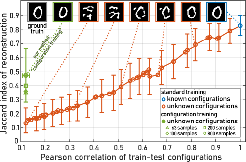
Figure 4: Reconstruction fidelity vs. the correlation between the test configurations and the training set configurations. The Jaccard index (JI), which quantifies the reconstruction fidelity, is plotted against the Pearson correlation coefficient (PCC) between the train and test configurations. For configurations with an average PCC of 0.12, our method of configuration training (green circle) produces higher-quality reconstructions than standard (single configuration) training, by a factor of $\approx 3.5$. The blue data point represents the JI for using the same fiber configuration for training and testing. The red curve shows the degradation of reconstruction fidelity with the decreasing correlation between the train and test set (see supplementary material). The green data points correspond to unknown fiber conformations using configuration training on 943 random fiber conformations. The effect of the training set size is observed by training separate models on 63/100/200/800 samples per configuration, with the average obtained JI depicted as the green triangle/diamond/square/circle. The standard deviation of the first three is emitted for clarity, and has the same size as the one that is shown. All points are calculated over the same test input patterns. The PCC between two different configurations corresponds to the average PCC between respective output intensity patterns for the same input excitations, and the standard deviation between the train and test for configuration training is shown. A representative example for the reconstruction of an unknown input digit is displayed at the top along with its ground truth.

To further examine the configuration training results, we show representative examples of test patterns in Figure 5, and in Visualization 2. In Figure 5, each column describes reconstructions from an arbitrary configuration, one from each day the data was acquired. Interestingly, the reconstructions for both known (part of the training) and unknown (only used for testing) configurations give results of similar quality. This is reflected by similar values which are obtained for known and unknown configurations over the entire test set using all of our evaluation metrics, as detailed in Table 1 of the supplementary material. We attribute the resemblance of the results for known and unknown configurations to the small number of examples in the train set from each configuration. More training data from each of the configurations could produce even better reconstructions. Moreover, the large standard deviation of the JI depicted in Figure 4 by the error bars is manifested in Figure 5, where evidently some digits are easier to reconstruct than others (e.g. ’1’ and ’6’ compared with than ’2’ and ’3’).

Figure 5: Reconstructions produced by configuration training of speckle from multiple low-correlated fiber conformations. The leftmost column shows the ground truth. Each of the other columns show reconstructions from a randomly chosen configuration, acquired at different days. The three (four) columns under “known” (”unknown confs”) depict reconstructions from configurations the model did (did not) train on. Noticeably, both known and unknown configurations results in reconstructions of similar fidelity. The Jaccard index of each reconstruction appears below it in blue, next to the pixel-wise accuracy which appears in orange.

4 Discussion

For a static fiber conformation accurate results can be obtained using a CNN with standard training, since similar digit images (e.g. two patterns of the digit ’9’) excite similar fiber modes. Thus, the resulting speckle for similar inputs within the same fiber conformation are spatially correlated, as shown in the blue histogram of Figure 6(a) for an input image of a ’9’. These correlations aid the CNN to produce accurate reconstructions, as evident in the top row of Figure 3(c) and the high JI described by the blue point of Figure 4. Furthermore, the relatively high correlations in the pixel basis hint that the simpler task of classifying the input digit images (according to digit) can potentially be achieved with a ”classical” machine learning approach, i.e. without DL. In [30], Li et al. used an unsupervised dimension reduction technique and demonstrated that speckle that emerge from thin diffusers can be clustered according to their original class or acquisition configuration. Here we take a similar approach and show that using the t-distributed Stochastic Neighbor Embedding (t-SNE) dimensionality reduction technique [36], images from the same fiber conformation are mostly clustered according to their underlying digit class (Figure 6(b)).

For a dynamic fiber that undergoes strong perturbations, one would not expect the CNN to work since even for the same images at the fiber input, speckle patterns for different fiber deformations show low correlations. However, the transmission properties cannot be totally uncorrelated, as it would have prevented the generalization over unknown conformations that we experimentally demonstrated in this study. To explore how we are able to produce high fidelity reconstructions, we search for invariant properties in the speckle produced for different fiber conformations. Following [20], we computed the correlations between output speckles for different configurations. For two random configurations, the speckle patterns that are obtained for different inputs exhibit a much narrower correlation distribution, which is centered around a much smaller value than within the same fiber conformation, as we depict in the orange histogram of Figure 6(a). This distribution is centered at $0.11\pm 0.01$, and presumably deems the mission of reconstruction from different configuration impossible. However, when we compare between the same inputs in random configurations, this distribution is slightly shifted to higher values, and centered at $0.12\pm 0.01$ (gray histogram of Figure 6(a)).

The observed decorrelation of the output intensity pattern in the pixel basis does not allow us to directly assess the level of disorder, since even if the transmission speckle decorrelates quickly when deformation is applied, some hidden information can still be present [13, 10]. We believe that the mere existence of these low, but non-zero correlations stand at the heart of the CNN’s success in the image reconstruction through unknown fiber conformations. Indeed, the 2D embedding of speckle patterns from different inputs and configurations using the t-SNE algorithm clusters the data points according to their original configuration. In Figure 6(c) we show a representative example for the embedding of 33 random configurations (with two configurations that completely overlap). We note that for less data, t-SNE is unable to differentiate between digits (Figure 6(d)) - a task the CNN succeeds at. The fact that configurations of the disorder can be discriminated using statistical analysis tools (Figure 6(c) and 6(d)) shows that the transmission properties of light are not totally randomized by the deformations, as outputs would otherwise be indistinguishable. This supports the interpretation that the deep learning model learns the invariant properties, common to all deformations, which are then used to infer and reconstruct the input excitation. We therefore conclude that there is an advantage to using DL when dealing with multiple conformations.

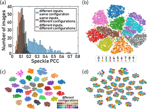
Figure 6: Speckle correlations and 2D embedding of inputs and configurations. (a) Histogram of the Pearson correlation coefficients of speckle for different DMD inputs within the same configuration (blue), speckle generated for the same DMD inputs in two different configurations (gray) and different inputs in two different configurations (orange). The blue histogram is wide and accounts for the ease of reconstructing images from a single fiber conformation. The shift of the mean value between the gray and orange histograms could account to the reason a CNN is able to generalize over fiber bends. (b) 2D embedding of 15k speckle patterns from a single fiber conformation mostly divides them according to the class of the digit that was displayed on the DMD (0-9). (c-d) 2D embedding of speckle patterns from 33 random configurations. The embedding contains 32 blobs, and an additional centered blob that corresponds to data that was not easily separable (which appears in the center due to the algorithm’s working mechanism). (c) The color code corresponds to different configurations (information that was not available to the algorithm), showing configuration clusters (with two configurations that completely overlap). (d) Same data as (c), the colors correspond to digits (same code as (b)), and shows that t-SNE is not successful in separating this data according to digits.

The fiber conformations we study in this work are driven by actuators that induce multiple bends on the millimeter scale. In real life applications, we expect fewer bends though on a longer length scale. We therefore compare the correlation between different fiber conformations, obtained for a few macro-bends and for the actuator-driven bends, and find that the PCC of the speckle output is $\approx 0.12$ in both cases (see supplementary material for more details). We therefore believe that the proposed configuration training can be implemented in real-life applications, and in particular for biomedical imaging, since the parameters of the fiber we use adhere to those used in prototype microendoscopes [6]. A note-worthy limitation of our work emerges from the homogeneity of the train set, which consists of a single class of images: digits. The CNN we use channels the input through an encoder, which represents the data in a smaller dimension called the latent space. Due to the homogeneity and the nature of encoders, code in the latent space would be decoded to a digit, or to a composition of digits, in the pixel space (the reconstruction). Thus, images from the same domain that is to be reconstructed should be used for the training of our model to achieve the best performance. However, this shortcoming can be easily overcome by utilizing a more complex DL model, which was shown to be able to generalize to images from other domains [18, 20].

5 Conclusion

In this work we experimentally demonstrated robustness to fiber deformations using a deep learning model. Our model is able to reconstruct images which are transmitted through a bent multimode fiber, with no knowledge of the specific fiber conformation, and regardless of the inflicted bend configuration. We presented an immense improvement in reconstruction fidelity compared with standard DL approaches, transforming an incomprehensible image to an intelligible one. We showed that to achieve generalization it is essential to train a CNN on the speckle patterns that originate from numerous fiber bends and are acquired for many different image inputs. We implemented such an approach by introducing configuration training. We then tested the network’s performance on patterns from strongly perturbed fibers, and showed good reconstruction results even for strong perturbations applied many weeks after the training process. Our demonstration has possible real-life applications, in particular for fiber endoscopy where changes in the geometrical configuration of the fiber are unavoidable. The CNN model we used is fairly simple and compact, with low memory requirements (compared to previous works in the field), allowing for video rate implementation with standard computers.

Supporting Information

See Supplement 1 for supporting content. See Visualization 1 for a few examples that provide a more extensive view of Figure 4, and Visualization 2 for more reconstruction examples using our configuration training. Supporting Information is available from the Wiley Online Library or from the author.

Acknowledgements

The authors kindly thank Snir Gazit for providing access to the computational resources which were used to train the neural networks, along with Ori Katz and Roy Friedman for many fruitful discussions and suggestions. SR and YB acknowledge the support of the Israeli Ministry of Science and Technology and the Zuckerman STEM Leadership Program. SMP is supported by the French Agence Nationale pour la Recherche (grant No. ANR-16-CE25-0008-01 MOLOTOF), the Labex WIFI (ANR-10-LABX-24, ANR-10-IDEX-0001-02 PSL*) and the France’s Centre National de la Recherche Scientifique (CNRS; France-Israel grant PRC1672). All authors acknowledge the support of Laboratoire international associé Imaginano.

References

- [1] D. J. Richardson, J. M. Fini, L. E. Nelson, Nature Photonics 2013, 7, 5 354.
- [2] L. G. Wright, D. N. Christodoulides, F. W. Wise, Science 2017, 358, 6359 94.
- [3] T. Čižmár, K. Dholakia, Nature Communications 2012, 3 1027.
- [4] S. Bianchi, R. Di Leonardo, Lab on a Chip 2012, 12, 3 635.
- [5] Y. Choi, C. Yoon, M. Kim, T. D. Yang, C. Fang-Yen, R. R. Dasari, K. J. Lee, W. Choi, Physical Review Letters 2012, 109, 20 203901.
- [6] S. Turtaev, I. T. Leite, T. Altwegg-Boussac, J. M. Pakan, N. L. Rochefort, T. Čižmár, Light: Science and Applications 2018, 7, 1.
- [7] S. Li, S. Horsley, T. Tyc, T. Čižmár, D. Phillips, arXiv 2020.
- [8] V. Tsvirkun, S. Sivankutty, K. Baudelle, R. Habert, G. Bouwmans, O. Vanvincq, E. R. Andresen, H. Rigneault, Optica 2019, 6, 9 1185.
- [9] S. M. Popoff, G. Lerosey, R. Carminati, M. Fink, A. C. Boccara, S. Gigan, Phys. Rev. Lett. 2010, 104 100601.
- [10] D. E. Boonzajer Flaes, J. Stopka, S. Turtaev, J. F. de Boer, T. c. v. Tyc, T. c. v. Čižmár, Phys. Rev. Lett. 2018, 120 233901.
- [11] S. Farahi, D. Ziegler, I. N. Papadopoulos, D. Psaltis, C. Moser, Optics Express 2013, 21, 19 22504.
- [12] A. M. Caravaca-Aguirre, E. Niv, D. B. Conkey, R. Piestun, Optics Express 2013, 21, 10 12881.
- [13] M. Plöschner, T. Tyc, T. Čižmár, Nature Photonics 2015, 9, 8 529.
- [14] D. Loterie, D. Psaltis, C. Moser, Optics Express 2017, 25, 6 6263.
- [15] L. V. Amitonova, A. P. Mosk, P. W. H. Pinkse, Opt. Express 2015, 23, 16 20569.
- [16] S. Li, C. Saunders, D. J. Lum, J. Murray-Bruce, V. K. Goyal, T. Čižmár, D. B. Phillips, Light: Science and Applications 2021, 10, 88.
- [17] S. Li, M. Deng, J. Lee, A. Sinha, G. Barbastathis, Optica 2018, 5, 7 803.
- [18] B. Rahmani, D. Loterie, G. Konstantinou, D. Psaltis, C. Moser, Light: Science and Applications 2018, 7, 1 1.
- [19] N. Borhani, E. Kakkava, C. Moser, D. Psaltis, Optica 2018, 5, 8 960.
- [20] Y. Li, Y. Xue, L. Tian, Optica 2018, 5, 10 1181.
- [21] P. Fan, T. Zhao, L. Su, Optics Express 2019, 27, 15 20241.
- [22] P. Caramazza, O. Moran, R. Murray-Smith, D. Faccio, Nature Communications 2019, 10, 1 1.
- [23] G. Barbastathis, A. Ozcan, G. Situ, Optica 2019, 6, 8 921.
- [24] B. Rahmani, D. Loterie, E. Kakkava, N. Borhani, U. Teğin, D. Psaltis, C. Moser, Nature Machine Intelligence 2020, 2 403.
- [25] T. Zhao, S. Ourselin, T. Vercauteren, W. Xia, Optics Express 2020, 28, 14 20978.
- [26] H. Chen, Z. He, Z. Zhang, Y. Geng, W. Yu, Optics Express 2020, 28, 20 30048.
- [27] C. Zhu, E. A. Chan, Y. Wang, W. Peng, R. Guo, B. Zhang, C. Soci, Y. Chong, Scientific Reports 2021, 11, 896.
- [28] Y. Liu, G. Li, Q. Qin, Z. Tan, M. Wang, F. Yan, Optics and Laser Technology 2020, 131 106424.
- [29] E. Kakkava, N. Borhani, B. Rahmani, U. Teğin, C. Moser, D. Psaltis, Applied Sciences 2020, 10, 11 3816.
- [30] Y. Li, S. Cheng, Y. Xue, L. Tian, Opt. Express 2020, 29, 2 2244.
- [31] S. Resisi, Y. Viernik, S. M. Popoff, Y. Bromberg, APL Photonics 2020, 5, 3 036103.
- [32] M. W. Matthès, Y. Bromberg, J. de Rosny, S. M. Popoff, arXiv 2020.
- [33] Y. LeCun, C. Cortes, MNIST handwritten digit database, http://yann.lecun.com/exdb/mnist/, URL http://yann.lecun.com/exdb/mnist/.
- [34] O. Ronneberger, P. Fischer, T. Brox, U-Net: Convolutional Networks for Biomedical Image Segmentation, 234–241, Springer International Publishing, ISBN 978-3-319-24574-4, 2015.
- [35] S. Resisi, Basic MNIST classifier model, https://github.com/shacharres/MNIST-classifier, URL https://github.com/shacharres/MNIST-classifier.
- [36] L. Van Der Maaten, G. Hinton, Journal of Machine Learning Research 2008, 9 2579.