Abstract

We introduce a soft computing approach for automatically selecting and combining indices from remote sensing multispectral images that can be used for classification tasks. The proposed approach is based on a Genetic-Programming (GP) framework, a technique successfully used in a wide variety of optimization problems. Through GP, it is possible to learn indices that maximize the separability of samples from two different classes. Once the indices specialized for all the pairs of classes are obtained, they are used in pixelwise classification tasks. We used the GP-based solution to evaluate complex classification problems, such as those that are related to the discrimination of vegetation types within and between tropical biomes. Using time series defined in terms of the learned spectral indices, we show that the GP framework leads to superior results than other indices that are used to discriminate and classify tropical biomes.

12 14 2267 Received: 17 June 2020; Accepted: 9 July 2020; Published: 15 July 2020 yes A Soft Computing Approach for Selecting and Combining Spectral Bands Juan F. H. Albarracín ¹, Rafael S. Oliveira ², Marina Hirota ^2,3, Jefersson A. dos Santos ⁴ and Ricardo da S. Torres ^5,* Juan F. H. Albarracín, Rafael S. Oliveira, Marina Hirota, Jefersson A. dos Santos and Ricardo da S. Torres Correspondence: ricardo.torres@ntnu.no; Tel.: +4792219307

1 Introduction

Remote sensing is important for monitoring and modeling vegetation dynamics and distribution in large-scale ecological studies. Most of the studies applying these techniques use multispectral indices that are based on a ratio (or some other simple mathematical relation) of the reflectance at two or more wavelengths Sims and Gamon (2003); Xue and Su (2017). These indices allow for complex data analyses, such as better detecting and visualizing specific targets, like vegetation vigour Ceccato et al. (2002); Zhang et al. (2015), water bodies Gao (1996), and deforestation patterns Schultz et al. (2016), since they make explicit complex interactions between the bands that cannot be evidenced individually.

The most commonly used indices, such as the Normalized Difference Vegetation Index (NDVI), give a broad and general view of many observable phenomena. Although these traditional measures are still widely used, they present limitations, among which we may point out the saturation of the NDVI for closed canopies, preventing the identification of vegetation heterogeneity. As pointed by Verstraete & Pinty Verstraete and Pinty (1996), spectral indices are very sensitive to the desired information and unresponsive to perturbing factors (such as soil color changes, relief, and atmospheric effects). Thus, they argue that more suitable indices should be designed for specific applications and particular instruments, as both the desired signal and the perturbing factors vary spectrally, and the instruments themselves only provide data for certain spectral bands. In this sense, most of the studies have focused on very specific applications or situations Gobron et al. (2000), i.e., most of them are very sensitive to new data and, thus, are not easily adaptable to different and possibly new applications or new datasets that are produced from diverse sensors.

Additionally, if the specific bands that are used for computing some indices are not available, they simply cannot be processed (e.g., the NDVI cannot be calculated from RGB images). Finally, most of the existing indices ignore available bands in multispectral images. In particular, land cover analysis is highly dependent on the sensor used for data acquisition Lu and Weng (2007). The ever growing variety of sensors with different technical specifications, such as spatial/spectral resolutions or acquisition protocols, may lead to low performance of traditional spectral indices, as they may not accurately reflect the same properties related to data obtained from different sources Xue and Su (2017). In all of those situations, the use of techniques that can learn existing patterns of interest from data can lead to more effective indices that are tailored to specific classification-dependent applications.

In this paper, we address those shortcomings by proposing a methodology that employs a Genetic-Programming (GP)-based framework for learning spectral indices that are specialized in discriminating pixels that belong to different classes. GP Koza (1992) is an evolution-based method that models candidate solutions for a problem as individuals of a population, and makes them evolve through generations. The objective is to find the best solutions for the target problem as the best individuals of the evolved population.

GP is widely known because of its capacity of effectively finding complex solutions to a great variety of problems, and because of its straightforward ability for parallel search Koza (1992). Perhaps, the most important property of GP is the interpretability of the solutions that are learned trough it, since it provides either math formulas or algorithms in a language that is predefined by the user. This property makes GP more suitable for spectral index learning than other evolutionary algorithms, because it can be designed to output formulas whose terms are spectral bands, combined through a set of operations that are defined by the user. The structure of the formula learned with GP can be further analyzed to determine the contribution of the spectral bands, and then induce high-level knowledge about the objects of study. The capacity of GP in solving a wide variety of complex problems is evidenced in a large volume of works that has successfully applied GP in uncountable domains Taleby Ahvanooey et al. (2019); Espejo et al. (2010); Nguyen et al. (2017); Khan et al. (2019).

Band selection and combination methods are important in multispectral scenery classification due to the well-known problem of the curse of dimensionality. The GP algorithm naturally selects and combines bands in a simultaneous fashion, as individuals in the population evolve. Hence, our method can be framed as a feature selection and extraction pipeline (rather than a merely band selection protocol) that projects multispectral images into a one-band feature space, yielded by the learned vegetation index. Even in the multispectral scenario, in which the few quantity of spectral bands suggests a lower risk of poor performance due to the curse of dimensionality, the selection of bands prevents classification flaws due to noisy bands.

We performed experiments to confirm our hypothesis related to the ability of Genetic-Programming-based vegetation indices (GPVI) for representing the canopy structural gradient between regions that can be either forests or savannas biomes, and the power of such index in extrapolating the classification of forest and savanna areas on a pixel basis for tropical South America, over time. We collected data from four multispectral sensors: Landsat 5 TM, Landsat 7 ETM+, MODIS MOD09A1.006 (Terra), and MODIS MYD09A1.006 (Aqua), forming monthly temporal series of the period between 2000 and 2016. Biomes are recognized as vegetation units of a particular physiognomy, which is the characteristic spatial arrangement and dominance of plant life forms that explain the vegetation general appearance lan Woodward et al. (2001); Woodward (2009). In summary, we target four research questions:

1. Are GP-based indices more effective than traditional indices in biome type classification tasks?

2. Would GP-based indices yield effective results when used in more complex classification problems such as those related to the discrimination of different vegetation types within the same biome?

3. Are GP-based indices suitable for time-series-based classification tasks?

4. What are the most frequently selected bands by using the GP-based discovery process?

It is important to state that this framework is not proposed to be a new land cover classification scheme. It is intended as a generic framework for guiding the identification of suitable combinations of spectral bands in remote sensing imagery, which may be used later in classification systems. To answer Q1, we compare classification performance on multispectral pixels projected by GPVI with respect to the ones projected by the widely used Normalized Difference Vegetation Index (NDVI) and Enhanced Vegetation Index (EVI). Furthermore, we handled two finer-scale classification problems, based on the discrimination of subcategories of savannas and forests with respect to its physiognomical structure and, thus providing an answer to Q2. Biomes are often subdivided into structural, compositional and/or functional subcategories (hereafter called “vegetation types”), according to plant phenological patterns (canopy leaf production and loss) or tree cover variation (canopy height and closure), among others. Analysis by vegetation type yields two sub-classes for forest (evergreen forests vs. semi-deciduous forests) and savannas (typical savannas vs. forested savannas). (In the context of this paper, we use the term forested savanna to refer to a tropical savanna biome which structurally resembles forests Ratnam et al. (2011).) To address Q3, taking advantage of the available temporal data, we perform experiments for whole-time-series classification and analysis, yielded by GPVI and the traditional indices. To address Q4, we analyze the structure of the learned spectral indices to determine the contribution of each band for classification.

2 Related Work

GP and other bio-inspired strategies have been used to develop spectral indices in a wide range of applications Su et al. (2017); Papa et al. (2016); Fonlupt and Robilliard (2000). Chion et al. Chion et al. (2008) proposed the genetic programming-spectral vegetation index (GP-SVI), a method that evolves a regression model to describe the nitrogen level in vegetation. A very similar work by Puente et al. Puente et al. (2011) introduced the Genetic Programming vegetation index (GPSVI) to estimate the vegetation cover factor in soils to assess erosion. Ceccato et al. proposed a new methodology to create a spectral index to retrieve vegetation water content from visible data Ceccato et al. (2002). Gerstmann et al. Gerstmann et al. (2016), in turn, introduced a method to find a general-form normalized difference index to separate cereal crops, through an exhaustive search in a set of possible permutations of bands and constants used in a general formula and measures effect size to determine class separability.

Spectral indices have demonstrated an ability to separate different classes of woody vegetation Liu et al. (2017). However, efforts that apply spectral indices for classification purposes normally rely on time series Costăchioiu and Datcu (2010); Löw et al. (2015); Prishchepov et al. (2012). A single value in time of the indices about an object of interest is not enough to discriminate it. This is particularly true in vegetation analysis since an object of interest can change its configuration seasonally. The possibility of novel indices that encode discriminative information invariant through time is open and could be achieved with our proposed technique. Balzarolo et al. Balzarolo et al. (2016) showed that, while using the NDVI index, there is a high correlation between the starting day of the growing season observed with MODIS data, and in-situ observations. Wang et al. Wang et al. (2017) developed a three-band vegetation index to minimize the snow-melt effect in monitoring spring phenology.

GP has also been used for classification. Ross et al. presented a method for mineral classification using three classes Ross et al. (2005). Rauss et al. Rauss et al. (2000) proposed evolving an index that returns values greater than $0$ when there is grass in the image, and values smaller than $0$, otherwise. In general, approaches for classification are applied in very close configurations like few classes or isolated binary cases. Regarding function learning for general purposes, GP has also been used to learn formulas to combine time series similarity functions Almeida and d. S. Torres (2017); Menini et al. (2019), or formulas that extract relevant information from similarity measures obtained throughout the user relevance feedback iterations Calumby et al. (2014), or textual sources Saraiva et al. (2013).

Different from the previous attempts, we propose a method that relies on how data are distributed in the space yielded by candidate indices, instead of driving the learning process exclusively to find indices that satisfy specific purposes (e.g., regression, classification). Albarracín et al. Hernández et al. (2016) explored the idea of learning spectral indices for classification tasks. Different from that work, here we conduct a comprehensive formal description of the GP-based index discovery framework. The objective is to guide researchers and developers in the creation of novel realizations and extensions of the proposed approach for managing multispectral data for different applications. To the best of our knowledge, this is one of the first works to describe experiments while using GP-based indices in such problems. We also add further analysis about the relevance of bands found in the learned vegetation indices. This may provide insights about the most important environmental processes that characterize each biome evaluated here. Finally, we introduce an optimized fitness function that is designed for a binary classification problem.

3 Learning Indices Based on Genetic Programming for Classification Tasks

In this section, we introduce the proposed GP-based index discovery framework and discuss its use in classification problems. First, we provide background on GP concepts (Section 3.1). Subsequently, we explain how GP is used to find suitable indices (Section 3.2). Finally, we discuss the use of GP-based indices in classification settings (Section 3.3). The whole pipeline is depicted in Figure 1.

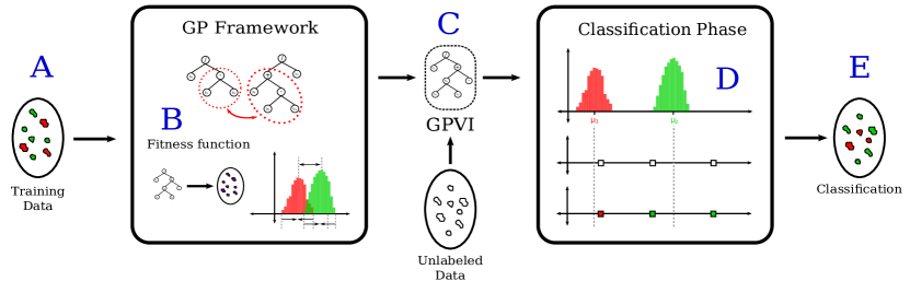
Figure 1: Genetic-Programming-based vegetation indices (GPVI) learning process and posterior classification framework for pixelwise discrimination. The labeled training set is represented by the set defined by part “A”. This ground truth is then used in the GP-based index discovery process in part “B”—see Sections 3.1 and 3.2. Classification is performed based on the best GP individual (GPVI) found—part “C”. This individual is used to define a score for unlabeled samples and to define the index distributions per class. Finally, unlabeled samples are assigned to the class whose distribution is the closest—part “E”.

3.1 Background on Genetic Programming

Genetic Programming (GP) is an artificial intelligence framework that is used for addressing optimization problems, based on the theory of evolution Koza (1992). GP represents candidate solutions to a problem as individuals within a population, which evolves over generations. The objective is to search for the best solutions (i.e., best individuals of the population) for the target problem, according to the Darwinian principle of survival of the fittest. In order to determine how fit an individual is to be selected, i.e., how good it solves the problem, a criterion must be defined in terms of a fitness function. This function has as input an individual, and outputs a score that allows for comparison of all the individuals in the population. This score determines the chance of individuals to be selected.

A typical representation of a GP individual relies on the use of a tree data structure, where leaf nodes (also known as terminals) represent operands and internal nodes encode functions, usually mathematical operators used to combine terminals. Figure 2 illustrates a typical GP tree representation, which encodes the function $f(a,b)=(a-b)\div(a+b)$, where $a$ and $b$ represent two terminals (variables or constants) and $+$, $-$, and $\div$ are the internal nodes.

Figure 2: Genotype (left) and phenotype (right) of a mathematical formula.

Figure 3 illustrates the typical evolutionary steps considered in the GP-based discovery process, which are outlined in Algorithm 1. GP starts with a randomly generated population of individuals (Line 1). The fitness of each individual is computed (Line 1) and a selection strategy is employed (Line 1) to determine which ones will be subjected to genetic operations. Typical operations include replication, mutation, and crossover. Each genetic operation has an associated occurrence rate, that determines how likely it is to be applied (Line 1). In replication (Line 1), individuals are selected to be placed in the population of the next generation, based on their scores. The diversity of candidate solutions in the population is maintained by mutation (Line 1), which is usually implemented as the substitution of a randomly selected node (operators or even a complete subtree can be selected to be changed) by a randomly generated new subtree. Finally, crossover (Line 1) is usually implemented as the exchange of subtrees from two other individuals (parents), which are selected based on their scores. The process of selecting individuals and applying genetic operators to form a new population of individuals is known as a generation (Line 1). The algorithm keeps iterating through generations until a stop condition is reached (Line 1), e.g., a pre-defined maximum number of generations. The best individual found so far is always preserved (Line 1), to be returned by the algorithm at the end.

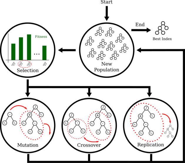
Figure 3: The general genetic programming process.

input : $pop\_size$, $nodes$, $P_{crossover}$, $P_{mutation}$, $P_{replication}$

output : $S_{best}$

1

2$Population\longleftarrow InitializePopulation(pop\_size,nodes)$

3 $EvaluatePopulation(Population)$

4 $S_{best}\longleftarrow GetBestSolution(Population)$

5while  $\neg$StopCondition() do

6       $Children\longleftarrow\emptyset$

7       while  $Size(Children)<population\_size$  do

8             $Operator\longleftarrow SelectOperator(P_{crossover},P_{mutation},P_{replication})$

9             if $Operator\equiv CrossoverOperator$ then

10                   $Parent_{1},Parent_{2}\longleftarrow SelectParents(Population,pop\_size)$

11                   $Child_{1},Child_{2}\longleftarrow Crossover(Parent_{1},Parent_{2})$

12                   $Children\longleftarrow Children\cup\{Child_{1},Child_{2}\}$

13             else if $Operator\equiv MutationOperator$ then

14                   $Parent_{1}\longleftarrow SelectParents(Population,pop\_size)$

15                   $Child_{1}\longleftarrow Mutate(Parent_{1})$

16                   $Children\longleftarrow Children\cup\{Child_{1}\}$

17             else if $Operator\equiv ReplicationOperator$ then

18                   $Parent_{1}\longleftarrow SelectParents(Population,pop\_size)$

19                   $Child_{1}\longleftarrow Replicate(Parent_{1})$

20                   $Children\longleftarrow Children\cup\{Child_{1}\}$

21            

22       end while

23      $EvaluatePopulation(Children)$

24       $S_{best}\longleftarrow GetBestSolution(Children,S_{best})$

25       $Population\longleftarrow Children$

26 end while

27return $S_{best}$

Algorithm 1 Typical Genetic Programming algorithm.

3.2 Gp-Based Index Discovery Process

3.2.1 Problem Definition

We apply the GP framework that is described in Section 3.1 to automatically learn spectral indices from remote sensing image (RSI) data. The GP-index discovery process relies on the definition of a training set composed of multispectral image pixels, which belong to distinct classes and their corresponding labels (e.g., savannas or forests). The framework is then used to evolve formulas, which represent mathematical equations combining the bands to find an index that successfully discriminates pixels belonging to the two classes.

3.2.2 Individual Representation

In our formulation, the spectral indices are computationally represented as a GP tree whose leaves are associated with RSI bands and the internal nodes, arithmetic operations. Figure 4 illustrates a GP individual, encoding the equation used to compute the Normalized Difference Vegetation Index (NDVI), defined in Equation (2).

Figure 4: Syntax tree representing the NDVI.

3.2.3 Discovery Process

The GP framework starts with a randomly generated population of indices (e.g., $b_{1}+b_{7}\times b_{2}$) that evolve as described above.

3.2.4 Fitness Computation

We devised a fitness function, which measures how well each GP individual (index) discriminates pixels from different classes. Each candidate index is used to combine bands of the pixels in the training set, associating one scalar with each one of them. With this information, we obtained index distributions that formed by the training pixels. Because the multi-band-image pixels used in the training set are labeled (i.e., for each pixel we know the class it belongs to), it is easy to determine how separated the distributions of indices of different classes are. The fitness of an individual is then computed based on the inter and intra-class distances in the training set of pixels: those of the same class should have similar index scores and should be far from pixels of the other class.

Algorithm 2 outlines the fitness computational process. First, we obtain the index distributions for each class (Lines 2 and 2), and we then compute the distance of the means of each distribution, normalized by their standard deviation (Line 2). Let $\mu_{a}$ and $\mu_{b}$ be the mean of all pixel values of, respectively, classes $a$ and $b$, and let $\sigma_{a}$ and $\sigma_{b}$ be their corresponding standard deviations. We defined the score of separability (fitness function) of the two classes as:

$$S=\displaystyle\frac{|\mu_{a}-\mu_{b}|}{\max\{\sigma_{a},\sigma_{b}\}}$$ (1)

The $\max$ function is used instead of the sum or product for the standard deviation values, because a small standard deviation of one of the classes could compensate the large standard deviation of the other, obtaining high separability values, even if both distributions would happen to overlap. This measure returns real numbers greater or equal than $0$. The larger the score, the better the separability. This fitness function is faster than the silhouette score, used in Hernández et al. (2016).

input : $population,X_{data},X_{labels}$

1

2for each $ind$ in $population$ do

3       $X_{ind}\leftarrow ApplyIndex(X_{data},ind)$

4       $X_{a}\leftarrow SelectDataOfLabel(X_{ind},a)$

5       $X_{b}\leftarrow SelectDataOfLabel(X_{ind},b)$

6       $S\leftarrow\displaystyle\frac{|\mu_{a}-\mu_{b}|}{\max\{\sigma_{a},\sigma_{b}\}}$

7       $AssignFitnessToIndividual(ind,S)$

8 end for

Algorithm 2 Fitness function

3.2.5 Selection Strategy

The score, associated with each individual by means of the fitness function described above, selects for individuals (see Lines 1, 1, and 1 of Algorithm 1) and applies the genetic operators on them. The selection strategy used is called tournament (Algorithm 3). Given an integer $k$ and the population, we randomly choose $k$ individuals, returning the best of them, according to their fitness.

input : $population,k$

output : $best$

1

2$best\leftarrow NIL$

3for $i=0$ to $k$ do

4       $i\leftarrow random(1,size(population))$

5       $ind\leftarrow population\big{[}i\big{]}$

6       if $best=NIL\vee getFitness(ind)>getFitness(best)$ then

7             $best\leftarrow ind$

8       end if

9      

10 end for

return $best$

Algorithm 3 Tournament selection

3.3 Using Gp-Based Indices in Classification Tasks

After we find a good index, we use it for classification. The class assignment process is based on the distribution of each class in the index space, through an algorithm known as Nearest Centroid Classifier (NCC) Manning et al. (2008) ([Ch. 14]), as outlined in Algorithm 4. First, we calculate the index values for all samples (Lines 4 and 4). Next, for the labeled samples, we calculate the mean value for each class (Line 4) and, for every validation example, we assign the label of the nearest class centroid (Line 4).

input : $X_{train},Y_{train},X_{val},vi$

output : $Y_{val}$

1

2$X_{train}\leftarrow ApplyIndex(X_{train},vi)$

3 $X_{val}\leftarrow ApplyIndex(X_{val},vi)$

4 $\mu\leftarrow CalculateCentroidsPerClass(X_{train},Y_{train})$

5 $Y_{val}\leftarrow empty\_list()$

6for each $x_{i}$ in $X_{val}$ do

7       $\mu_{i}\leftarrow FindNearestCentroidLabel(x_{i},\mu)$

8       $AppendToList(Y_{val},\mu_{i})$

9 end for

return $Y_{val}$

Algorithm 4 Nearest Centroid Classifier

3.4 Computational Complexity

The computational complexity of the GP-based index discovery process is $O(G\times N\times E)$, where $G$ is the number of generations, $N$ is the number of individuals in the population, and $E$ is the fitness evaluation time. The calculation time of the fitness function for each individual (see Equation (1)) increases linearly with the number of samples used to calculate the distance between the distributions. Thus, $E$ is determined by the complexity of an individual (e.g., its size $S$) and the number of training samples ($n$), which leads to a total time complexity of GP training experiment of $O(G\times N\times S\times n$). Note that this GP learning state is performed once for a given training dataset and an off-line operation. The application of the learned index on unseen spectral data is performed in constant time, similarly to the traditional vegetation indices.

4 Experiments and Results

In this section, we separately address the research questions, stated in Section 1. Therefore, each question is addressed in a specific subsection, which presents the adopted experimental protocol, used datasets (when necessary), and achieved results.

Additionally, we provide a set of experiments that are orthogonal to the ones that involve the data from Tropical South America (Q1, Q2, Q3, and Q4). In these experiments, we test sensor invariance in GPVI, i.e., how robust is our method when tested on different sensors. Therefore, all experiments presented in Sections 4.1–4.4 consider results that are related to the use of two families of sensors: Landsat and MODIS.

4.1 Gpvi for Broad-Scale Biome Classification

In this section, we address Q1 by performing experiments for the forest/savanna discrimination problem on raw (non-temporarily ordered) pixels, in which traditional vegetation indices (e.g., NDVI, EVI, and EVI2) are widely used.

4.1.1 Data Acquisition and Pre-Processing

The selected study sites are distributed across the region, comprising South American tropical savannas and forests (Figure 5). These locations correspond to 250 m $\times$ 250 m areas with the centroids imported from a subset of the inventory data used by Dantas et al. Dantas et al. (2016). Each of these points is visually assessed using Google Earth (GE) images from 2016, superimposed with MODIS grid cells of the same size while using Series Views Freitas et al. (2011). The geographical coordinates used as ground truth are defined in terms of whether the MODIS pixel at which the points fall into are completely filled with the vegetation type consistent with the corresponding labeled biome (i.e., savanna or forest) and vegetation types, as determined during the field work campaigns. Pixels that are not entirely filled with the corresponding biome type (e.g., due to deforestation and conversion to other land uses) are either replaced by a neighboring pixel fulfilling these criteria or discarded (when a nearby suitable pixel could not be found).

The data were acquired using the Google Earth Engine (GEE) API to download the scenes containing the study areas along the time. Two different data products from different sensors were downloaded:

Landsat Surface Reflectance sensors(Landsat) (https://www.usgs.gov/products/data-and-tools/gis-data (As of 3rd March 2020)): we merged data from Landsat 5 Thematic Mapper (TM), and Landsat 7 Enhanced Thematic Mapper Plus (ETM+), as suggested by Kovalskyy and Roy Kovalskyy and Roy (2013), in order to alleviate the lack of data availability due to the Landsat 7 ETM+ scan line failure in 2003. The GGE API retrieves the data form the United States Geological Survey (USGS), which provides Level-1 terrain-corrected (L1T) products, and already pre-processes the scenes regarding cloud detection (with the fmask algorithm Zhu and Woodcock (2012)), geo-referencing, and atmospheric correction.

Moderate Resolution Imaging Spectroradiometer (MODIS): here, the data from the satellite products MOD09A1.006 (Terra) (https://lpdaac.usgs.gov/products/mod09a1v006/ (As of 3rd March 2020)) and MYD09A1.006 (Aqua) (https://lpdaac.usgs.gov/products/myd09a1v006/ (As of 3rd March 2020)) were also merged. According to the specifications, (https://nsidc.org/data/modis/terra_aqua_differences (As of 24th February 2020)) the differences between the two satellites do not involve the nature of data collected in the bands considered in this study. Data with the blue band greater than 10% of its maximum value and/or the sensor view zenith angle greater than $32.5^{\circ}$ were excluded, as discussed by Freitas et al. Freitas et al. (2011).

The data are available at 250 m/pixel for all the bands in the LANDSAT sensors, and only in bands 1 and 2 of the MODIS ones, while, for bands 3 to 7, the spatial resolutions is of 500 m/pixel. As GEE lets the users define the spatial resolution of the data to be acquired, each area was covered exactly by one pixel in LANDSAT. In MODIS, bands 3–7 contain information of the surrounding region of each one of the areas. For each area, we downloaded a time series, corresponding to the period covered from January, 2000 to August, 2016. In order to fill gaps (principally due to the Landsat 7 failure in 2003), the data were composite into monthly time series and is subsequently linearly interpolated.

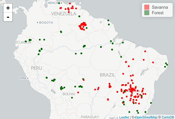
Figure 5: Geographical distribution of the areas considered in Tropical South America, corresponding to the data collected for training and validation. Imported form Dantas et al. (2016).

Table 1 presents information about the bands downloaded for both sensors, Landsat (https://www.usgs.gov/faqs/what-are-best-landsat-spectral-bands-use-my-research (As of 3rd March 2020)) and MODIS, associating the channel name with the band code and specifying the wavelength range covered by the band. We selected the channels blue, green, red, near infrared (NIR) 1 and 2, and short-wave infrared (SWIR) 1 and 2. Landsat TM products also normally provide information for the thermal infrared spectral region (LWIR), corresponding to band number 6. However, these specific SR products do not include this information.

Table 1: Specification of spectral bands for sensors Landsat and MODIS.

	Landsat		MODIS
Name		$\lambda$ ($\upmu$m)		$\lambda$ ($\upmu$m)
Blue	B1	0.45–0.52	B3	0.46–0.48
Green	B2	0.52–0.60	B4	0.55–0.57
Red	B3	0.63–0.69	B1	0.62–0.67
NIR	B4	0.76–0.90	B2	0.84–0.88
NIR 2	-	-	B5	1.23–1.25
SWIR	B5	1.55–1.75	B6	1.63–1.65
SWIR 2	B7	2.08–2.35	B7	2.11–2.16

4.1.2 Baselines

The indices learned through the proposed method (GPVI) are compared to three of the most widely used vegetation indices to characterize forests and savannas Viña et al. (2011). Hereafter we will refer to these three methods as our baselines:

Normalized difference vegetation index (NDVI): normalized difference between the red and near infrared channels to measure vegetation greenness Rouse et al. (1974).

$$NDVI=\displaystyle\frac{NIR-Red}{NIR+Red}$$ (2)

Enhanced vegetation index (EVI): enhancement of sensitivity adding the blue channel Huete et al. (2002). Proposed to improve saturation problems occurring in NDVI, when representing forest heterogeneity.

$$EVI=\displaystyle\frac{2.5\times(NIR-Red)}{NIR+6.0\times Red-7.5\times Blue+1}$$ (3)

Two-band enhanced vegetation index (EVI2): calibration of EVI so it must not depend on the blue band, particularly because the blue band is not included in products of old sensors and normally presents noise problems Jiang et al. (2008).

$$EVI2=\displaystyle\frac{2.5\times(NIR-Red)}{NIR+2.4\times Red+1}$$ (4)

4.1.3 GP Configuration

Table 2 shows a summary of the configuration of the GP algorithm. The parameters of the formulas (i.e., leaves of the trees) are random real numbers between $0$ and $10^{3}$, and the variables are spectral bands. The possible operators of the formula (i.e., internal nodes) are addition ($+$), subtraction ($-$), multiplication (*), protected division ($\%$), protected square root ($srt()$), and protected natural logarithm ($rlog()$), as suggested by Koza Koza (1992) in order to avoid division by zero, imaginary roots, and logarithm of negative numbers.

Table 2: Genetic Programming (GP) parameters setup. The three last operators mentioned stands for protected division ($\%$), protected square root ($srt()$) and protected natural logarithm ($rlog()$).

Parameter	Value
Population size	100
Generations	200
Operators (intern nodes)	{+, -, *, %, srt(), rlog()}
Parameters (laves)	$\{b_{i}:0\leq i<n\}\cup\{c_{j}\in[0,10^{3}]\}$
Maximum initial tree depth	6
Selection method	Tournament $\times\ 3$
Crossover rate	$0.9$
Mutation rate	$0.1$

The experiments were performed with $100$ individuals and $200$ generations. New randomly generated trees will not have a depth greater than 6. The selection method is tournament with three individuals. It consists of randomly selecting three individuals from the population and allowing the best one to go to crossover, as many times as a new population is completed. Once two individuals are chosen, they have a probability of $0.9$ to cross their genetic information and create new individuals. Every new individual in the population has a probability of $0.1$ to mutate. The algorithm must stop when $200$ generations are reached. The learning process for all classification problems using this configuration converged correctly, so more complex configurations, e.g., more iterations or a higher number of generations were not likely to improve performance.

4.1.4 Evaluation Protocol

GPVI is optimized to discriminate raw pixels, rather than whole time series. We considered the pixels only corresponding to the first five years (from 2000 to 2004) of the collected time series as training set for the GP framework, without preserving their temporal relation, since GPVI is intended to be time-independent. Thus, each pixel in each location (281 in total) and time stamp (12 months $\times$ five years) is a sample. Once obtained, the GPVI is used to classify the rest of the data, used as test set. The classification performance on the test set (from 2005 to 2016) is reported in the following section.

4.1.5 Results

The performance of GPVI and the indices used as baselines are summarized in Table 3. The columns marked with Prod., User, and Acc. correspond to the producer’s, user’s, and normalized accuracies, respectively. The producer’s accuracy for each class is the rate of correctly classified samples that belong to that class, while the user’s accuracy is the rate of correctly classified samples that are classified by the system as such. The normalized accuracy is the average of the producer’s accuracy of all the classes, which is a total accuracy (rate of correctly classified samples) giving all of the classes the same weight, regardless of the number of samples that belong to each one. The results obtained for Landsat and MODIS sensors can be contrasted.

Table 3: Normalized accuracy (Acc.) and user’s (User) and producer’s (Prod.) accuracy per class for forest/savanna discrimination.

	Landsat					MODIS
	Forest		Savanna			Forest		Savanna
	Prod.	User	Prod.	User	Acc.	Prod.	User	Prod.	User	Acc.
NDVI	89.28	86.60	90.49	92.44	89.89	78.71	80.19	86.44	85.37	82.58
EVI	87.75	85.64	89.88	91.42	88.81	80.90	83.79	89.10	86.98	85.00
EVI2	87.34	85.14	89.48	91.10	88.41	78.24	81.90	87.93	85.27	83.09
GPVI	96.38	93.59	95.46	97.46	95.92	88.30	86.16	91.09	91.08	89.69

The baselines presented similar performances and were clearly outperformed by GPVI ($6\%$ better as compared to Landsat and $4\%$ to MODIS). In general, the performance for Landsat was better than the one for MODIS, and the rate of correctly classified savannas was higher than the rate of correctly classified forests. Regarding user’s accuracy, a clear superiority of GPVI over the baselines was observed.

It is important to remark that a lower performance of GPVI and the baselines is expected for MODIS, as bands 3 to 7 have lower spatial resolution, which forced the data collection process to include information of the surrounding of the areas, which can be considered as noise.

An additional experiment tests the confidence of the classification of the spectral indices. For this, we took the one-band pixel values, yielded by each spectral index, for all of the locations, trained a Logistic Regression classification algorithm with them Hastie et al. (2001) ([Ch. 4]), and used its predicted class probability given a data point as a confidence score, since the class that is assigned to the areas depends on whether this value is under or over $0.5$. Thus, scores that are close to this value are more likely to be classified incorrectly, since the algorithm is totally uncertain of the class that it assigns to the sample. Figures 6 and 7 show scatterplots of mean accuracy vs. mean confidence score obtained in each area, for Landsat and MODIS, respectively. It can be seen that GPVI presented, on average, higher confidence values than the baselines, which means less confusion at classification time. The fact that savannas and forest can transit into each other’s states Dantas et al. (2016), can explain those areas that, in general, obtained low confidence and low accuracy, since a transitional location presents features of both biomes, leading to a higher confusion in the classification algorithm. Those areas presenting low accuracy and high confidence in various experiments could also result from mislabeled samples.

NDVI

EVI

EVI2

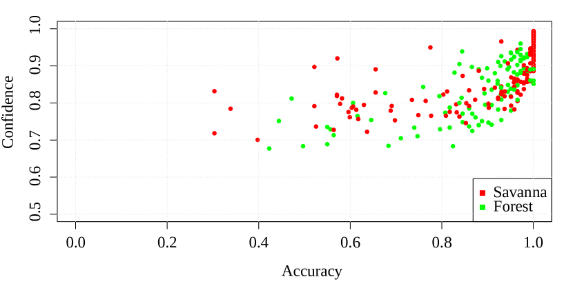
GPVI

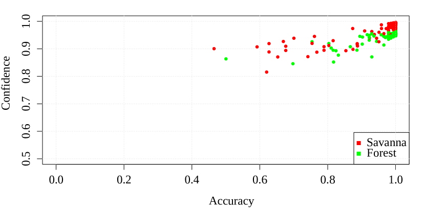
Figure 6: Confidence vs. accuracy in each area (Landsat).

NDVI

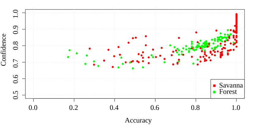
EVI

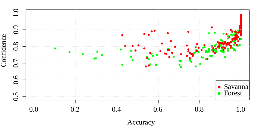
EVI2

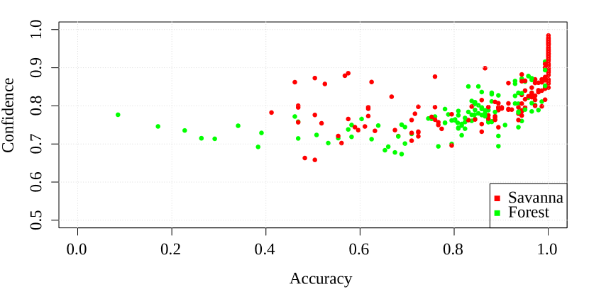
GPVI

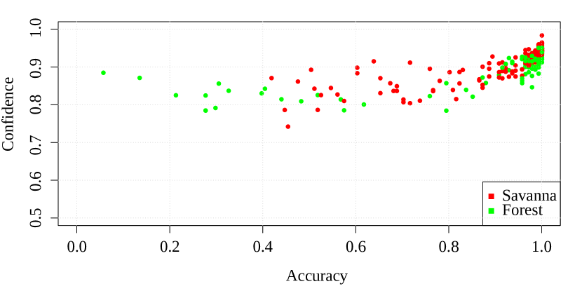
Figure 7: Confidence vs. accuracy in each area (MODIS).

4.2 Gpvi for Finer-Scale Vegetation Type Classification

To address Q2, we consider two separate classification problems that are harder than forest/savanna discrimination, as they deal with the discrimination of vegetation types (subcategories of savannas and forests with respect to their physiognomy): evergreen vs. semi-deciduous forests, and typical vs. forested savannas. In this setting, traditional indices often saturate and, normally, are not even considered in analyses, because they lack representation of within-biome differences (i.e., they consider the whole biome as an homogeneous landscape) Xue and Su (2017); Viña et al. (2011); Schultz et al. (2016).

The data used for this set of experiments, as well as the baselines, the parameters used in the GP framework, and the evaluation protocol, are exactly the same as the ones that are used for the forest/savanna classification problem (Section 4.1).

The performance of GPVI and the indices used as baselines are summarized in Tables 4 and 5. The results obtained for Landsat and MODIS sensors can be contrasted.

Table 4: Normalized accuracies (Acc.) and user’s (User), and producer’s (Prod.) accuracies per class for evergreen forest (EGF)/semi-deciduous forest (SDF) discrimination.

	Landsat					MODIS
	EGF		SDF			EGF		SDF
	Prod.	User	Prod.	User	Acc.	Prod.	User	Prod.	User	Acc.
NDVI	67.04	92.94	39.95	9.18	53.50	75.17	75.00	61.61	12.95	68.39
EVI	64.50	95.21	61.38	12.72	62.94	72.19	96.73	63.39	13.02	67.79
EVI2	63.93	94.55	56.61	11.61	60.27	69.95	96.41	61.08	12.20	65.52
GPVI	78.40	96.03	61.90	19.34	70.15	84.44	98.51	78.72	23.21	81.58

Table 5: Normalized accuracies (Acc.) and user’s (User), and producer’s (Prod.) accuracies per class for typical savanna (TS)/forested savanna (FS) discrimination.

	Landsat					MODIS
	TS		FS			TS		FS
	Prod.	User	Prod.	User	Acc.	Prod.	User	Prod.	User	Acc.
NDVI	57.92	96.96	73.70	10.60	65.81	59.89	96.80	70.99	10.88	65.44
EVI	58.37	96.17	65.61	9.72	61.99	62.91	96.03	62.28	10.33	62.60
EVI2	58.36	96.17	66.17	9.71	62.27	62.68	96.01	62.48	10.26	62.58
GPVI	71.06	97.66	74.89	14.98	72.98	58.62	97.32	76.34	11.28	67.48

For the evergreen forest/semi-deciduous forest discrimination (Table 4), the baselines presented similar performances when compared to GPVI, except for NDVI from Landsat, which presented a much inferior performance than the other baselines. In general, the baselines behaved similarly for both sensors, and they were outperformed by GPVI by about $7\%$ for Landsat, and by approximately $13\%$ for MODIS. The performance of GPVI using MODIS data was much higher than Landsat, and evergreen forest was classified with a higher rate of correctly classified areas. The user’s accuracy shows an evident bias towards the class evergreen forest for all of the indices. However, this bias is slightly lower for GPVI.

For the typical savanna/forested savanna discrimination (Table 5), the baselines presented similar performances for both sensors, and they were outperformed by GPVI by about $7\%$ for Landsat, and by about $2\%$ for MODIS. The performance of GPVI using Landsat data was superior than using MODIS, and forested savanna obtained a higher rate of correctly classified areas only for Landsat; for MODIS, both classes obtained similar rates. The user’s accuracy shows an evident bias towards typical savannas for all of the indices. However, this bias is slightly lower for GPVI.

4.3 Gpvi for Time-Series Analysis And Classification

To address Q3, we apply GPVI, along with the baselines, to the data collected, but now maintaining its temporal relation. Therefore, we are now not working with raw pixels, but with whole time series. For this set of experiments, there was no index-learning (i.e., training) stage, since we took the same indices that were learned in the experiments for raw-pixel-based forest/savanna classification (Section 4.1), and evergreen forest/semi-deciduous forest and typical savanna/forested savanna classification (Section 4.2). The only difference now is that they will be applied to the multispectral time series in order to yield one-dimensional time series.

The data used for this set of experiments, as well as the baselines, are exactly the same as the ones used for the raw-pixelwise forest/savanna classification problem (Section 4.1).

4.3.1 Experimental Protocol

We use a slightly different protocol from the raw-pixel classification experiments, due to the amount of data available. For pixel classification, each pixel ($281$ in total) in each location at each time stamp ($12$ months $\times$ 5 years) is a sample, so there are enough data ($281\times 12\times 5=$ 16,860) to provide a reliable comparison between GPVI and other indices. For time series classification, on the other hand, the number of samples is substantially smaller, 25 areas had to be discarded due to a large amount of gaps, preventing a reliable linear interpolation to fill them. This yields $256$ areas, which means a sample of $256$ sites and, thus, a cross validation protocol is used.

We apply the GPVIs learned in the raw-pixel-classification phase on the time series of multispectral pixels to yield a one-dimensional time series per pixel. We do the same with the baseline indices. The resulting series are used as an input of a time-series classification scheme.

The time series classification set-up considers the entire time series of each area as a sample, and splits the datasets to settle a $5\times 2$-fold cross validation protocol. In this protocol, we randomly sample half of the series, preserving class distribution, and use this half to train our classification algorithm; the other half is used for validation. The subsets are then swapped (the one used for training was now used for validation and vice-versa). This process is repeated five times, which results in a total of ten classification experiments.

We use the well-known 1-NN with Dynamic Time Wrapping (DTW) distance Berndt and Clifford (1994) time-series classification algorithm to perform the experiments. We performed a series of statistical tests in order to compare GPVI with each one of the baselines, as suggested by the literature on classification algorithms Demšar (2006); Dietterich (1998). First, we performed a Friedman test, a non-parametric test across multiple measures, which, in this case, are each one of the $5\times 2$-fold accuracies from GPVI and the three baselines. We complemented our analysis with Wilcoxon Signed Rank tests among every pair of methods. This test can only be done between two sets of experiments, while assuming that each experiment in a population is paired to another experiment of the other population, and it is also non-parametric. For the Friedman and Wilcoxon tests, we considered a significance level of $0.05$. Finally, to not underestimate the $p$-values yielded by the Wilcoxon tests, we applied Bonferroni post hoc adjustment on the obtained $p$-values.

Up to this point, we have shown the effectiveness of GPVI for pixelwise discrimination, without considering temporal information. However, in this section, we show how it behaves using time series, first with a visual comparison of GPVI with the other indices and then with the time-series classification set-up described above.

4.3.2 Time Series Analysis by Visual Assessment

The time series for GPVI and the baselines are graphically represented, taking the mean of the pixel values of all areas from the same class in each time stamp, so it is desirable that the curves corresponding to different classes are far away from each other. The instantaneous standard deviation of each class are also shown around the corresponding curve, only for the forest-savanna discrimination, for visualization purposes, since the other classification problems presented less separability. It is important to point that, since GPVI is learned with many degrees of freedom, the values are not necessarily bounded like NDVI, for example, comprising values between $-$1 and 1.

Figures 8 and 9 show the time series for Landsat and MODIS, respectively, in the forest/savanna classification problem. Landsat data present a greater separation between the series than MODIS, for GPVI and the baselines. It is clear how GPVI makes it easier to discriminate the values of pixels for the two classes, regardless of the time stamp.

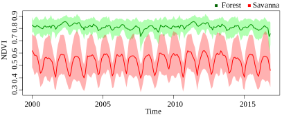
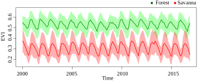
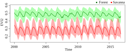
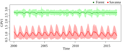
Figure 8: Time series for forest/savanna discrimination (Landsat). Shaded areas indicate the standard deviation of the index scores among all the data points for a given timestamp.

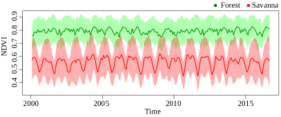
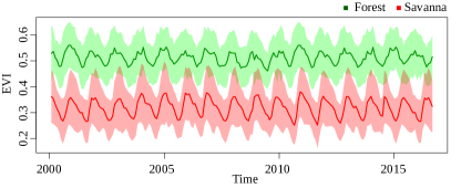
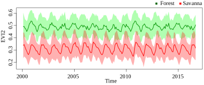
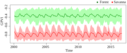
Figure 9: Time series for forest/savanna discrimination (MODIS). Shaded areas indicate the standard deviation of the index scores among all of the data points for a given timestamp.

The next classification problem corresponds to evergreen forest/semi-deciduous forest. Figures 10 and 11 show the time series for Landsat and MODIS, respectively. Although the separation of GPVI is not as good as it was in the forest/savanna problem, it is still better than the baselines. Moreover, the difference between sensors is also not as evident.

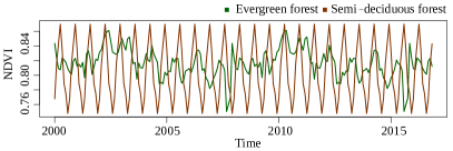
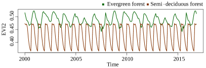
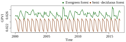
Figure 10: Time series for evergreen forest/semi-deciduous forest discrimination (Landsat).

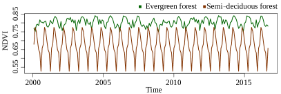
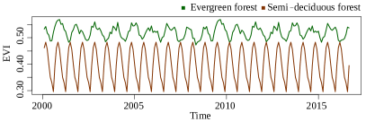
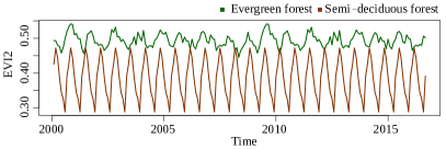
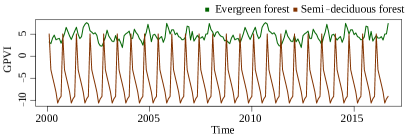
Figure 11: Time series for evergreen forest/semi-deciduous forest discrimination (MODIS).

Figures 12 and 13 show the time series for Landsat and MODIS, respectively, for the typical savanna/forested savanna savanna classification problem. The separation of the classes for all indices was worse than the other classification problems, showing that discriminating between these two classes is a hard problem—at least with the available spectral information.

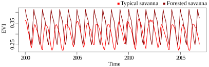
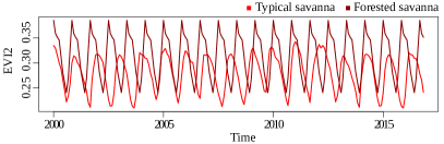
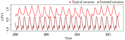
Figure 12: Time series for typical savanna/forested savanna discrimination (Landsat).

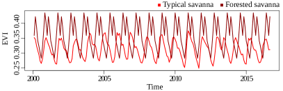
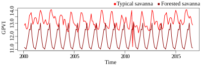
Figure 13: Time series for typical savanna/forested savanna discrimination (MODIS).

4.3.3 Time Series Classification Performance

Table 6 shows the normalized accuracy values that were obtained in the experiment corresponding to the forest/savanna time series discrimination for both sensors, as well as the user’s and producer’s accuracy. The Friedman test p-value associated with Landsat is $3.67\times 10^{-5}$, and with MODIS was $7.28\times 10^{-2}$, showing that, for both sensors, there was a significant statistical difference. However, the corrected pairwise tests show that there is no significant difference between GPVI and NDVI for Landsat. For MODIS, the tests show no significant difference between GPVI and EVI/EVI2.

Table 6: Normalized accuracies and user’s and producer’s accuracies per class for forest/savanna time series discrimination. $\blacktriangle$ means that GPVI was statistically superior to the corresponding baseline; $\blacktriangledown$, which it was statistically inferior, and $\bullet$, which both methods were tied.

		Forest		Savanna		Total
Sensor	Index	Producer	User	Producer	User	Accuracy
Landsat	NDVI	$98.23\pm 2.20$	$99.63\pm 0.79$	$99.26\pm 0.64$	$98.96\pm 1.49$	$\bullet~{}98.75\pm 0.98$
	EVI	$94.71\pm 2.80$	$98.36\pm 1.57$	$98.48\pm 1.14$	$96.62\pm 1.78$	$\blacktriangle~{}96.60\pm 1.05$
	EVI2	$94.69\pm 1.37$	$98.34\pm 1.98$	$98.13\pm 2.01$	$97.22\pm 1.59$	$\blacktriangle~{}96.41\pm 1.45$
	GPVI	$99.10\pm 0.95$	$99.62\pm 0.81$	$99.64\pm 0.59$	$99.48\pm 0.92$	$~{}~{}~{}99.37\pm 0.36$
MODIS	NDVI	$92.30\pm 3.47$	$91.72\pm 3.74$	$94.34\pm 1.91$	$98.68\pm 2.57$	$\bullet~{}93.32\pm 1.60$
	EVI	$95.73\pm 1.86$	$93.82\pm 2.09$	$95.13\pm 2.14$	$96.59\pm 2.18$	$\bullet~{}95.43\pm 1.60$
	EVI2	$95.57\pm 2.19$	$93.58\pm 2.81$	$94.83\pm 2.30$	$95.28\pm 2.51$	$\bullet~{}95.20\pm 1.42$
	GPVI	$94.80\pm 1.91$	$92.37\pm 3.23$	$94.20\pm 1.57$	$93.39\pm 2.65$	$~{}~{}~{}94.50\pm 1.46$

Table 7 shows the normalized accuracy values that were obtained in the experiment corresponding to the evergreen forest/semi-deciduous forest time-series discrimination for both sensors, as well as the user’s and producer’s accuracy. The Friedman test p-value for Landsat was $0.2$ and, for MODIS, was $0.4$, showing that there is no significant difference among all of the indices in general. The corrected pairwise tests show the same result. Unlike the forest/savanna problem, results using MODIS dataset shows better results than results with Landsat.

Table 7: Normalized accuracies and user’s and producer’s accuracies per class for evergreen forest/semi-deciduous forest time series discrimination. $\blacktriangle$ means that GPVI was statistically superior to the corresponding baseline; $\blacktriangledown$, which it was statistically inferior, and $\bullet$, which both methods were tied.

		Evergreen Forest		Semi-Deciduous Forest		Total
Sensor	Index	Producer	User	Producer	User	Accuracy
Landsat	NDVI	$93.72\pm 4.09$	$94.76\pm 6.64$	$23.69\pm 24.84$	$57.95\pm 34.31$	$\bullet~{}58.70\pm 13.28$
	EVI	$94.59\pm 3.68$	$96.28\pm 4.33$	$40.10\pm 31.82$	$39.52\pm 28.71$	$\bullet~{}67.34\pm 16.20$
	EVI2	$94.25\pm 3.00$	$97.29\pm 1.93$	$41.50\pm 25.46$	$39.29\pm 30.20$	$\bullet~{}67.88\pm 12.56$
	GPVI	$96.31\pm 3.71$	$97.27\pm 3.47$	$54.00\pm 27.43$	$29.29\pm 28.99$	$~{}~{}~{}75.16\pm 13.50$
MODIS	NDVI	$95.16\pm 2.41$	$96.41\pm 4.53$	$48.67\pm 32.48$	$42.17\pm 14.97$	$\bullet~{}71.91\pm 15.77$
	EVI	$96.29\pm 2.57$	$98.09\pm 1.26$	$68.33\pm 23.32$	$44.50\pm 17.20$	$\bullet~{}82.31\pm 11.16$
	EVI2	$96.10\pm 2.30$	$98.46\pm 1.22$	$68.33\pm 30.24$	$46.50\pm 19.96$	$\bullet~{}82.22\pm 14.39$
	GPVI	$97.19\pm 2.45$	$97.73\pm 1.72$	$65.45\pm 31.74$	$47.50\pm 22.73$	$~{}~{}~{}81.32\pm 14.85$

Table 8 shows the normalized accuracy values that were obtained in the experiment corresponding to the typical savanna/forested savanna time series discrimination for both sensors, as well as the user’s and producer’s accuracy. The Friedman test p-value for Landsat is $6.67\times 10^{-4}$ and, for MODIS, is $0.23$, showing that only for Landsat there was a significant difference. The corrected pairwise tests evidence the superiority of GPVI as compared to EVI2 only for Landsat. For this classification problem, both sensors obtained a similar performance.

Table 8: Normalized accuracies and user’s and producer’s accuracies per class for typical savanna/forested savanna time series discrimination. $\blacktriangle$ means that GPVI was statistically superior to the corresponding baseline; $\blacktriangledown$, which it was statistically inferior, and $\bullet$, which both methods were tied.

		Typical Savanna		Forested Savanna		Total
Sensor	Index	Producer	User	Producer	User	Accuracy
Landsat	NDVI	$94.55\pm 2.55$	$94.56\pm 1.41$	$20.83\pm 19.71$	$18.50\pm 11.95$	$\bullet~{}57.69\pm 10.04$
	EVI	$94.26\pm 2.73$	$94.15\pm 3.34$	$14.86\pm 12.38$	$12.67\pm 18.78$	$\bullet~{}54.56\pm 6.26$
	EVI2	$93.32\pm 2.66$	$94.42\pm 3.50$	$0.00\pm 0.00$	$11.83\pm 10.44$	$\blacktriangle~{}46.66\pm 1.33$
	GPVI	$95.13\pm 2.91$	$92.38\pm 2.03$	$31.20\pm 26.48$	$12.67\pm 16.24$	$~{}~{}~{}63.16\pm 12.66$
MODIS	NDVI	$94.20\pm 2.60$	$95.25\pm 1.63$	$11.56\pm 8.83$	$5.33\pm 8.64$	$\bullet~{}52.88\pm 5.13$
	EVI	$94.26\pm 2.62$	$98.24\pm 1.06$	$26.42\pm 31.94$	$12.33\pm 11.66$	$\bullet~{}60.34\pm 16.18$
	EVI2	$94.32\pm 2.79$	$98.12\pm 1.35$	$16.58\pm 17.16$	$5.67\pm 9.17$	$\bullet~{}55.45\pm 9.35$
	GPVI	$94.42\pm 2.18$	$94.23\pm 2.93$	$30.13\pm 27.99$	$18.33\pm 20.68$	$~{}~{}~{}62.28\pm 13.80$

4.4 Study on the Structure of the GPVIs

To address Q4, we analyze the relevance that GPVI assigns to the bands and operators to attain a good classification, by counting the most frequent formula elements in the top 10-indices obtained in the last population of the GP framework, for the raw-pixel classification experiments (Sections 4.1 and 4.2). We compare the structure of the indices learned in Landsat and MODIS, and the relevance of the associated bands for both sensors in order to check whetherthey match or not.

4.4.1 Experimental Protocol

As mentioned before, we considered the results of the raw-pixel classification experiments and, for each classification problem, we extracted the 10 indices with the best performance that our GP framework found. While using the tree representation of the indices, we extracted all of the possible subtrees (one per inner node), corresponding to the subexpressions of a given formula. We then count and rank the subexpressions, and perform two analyses on this data: in the first one, we build frequency histograms of all of the bands and compare the histograms yielded on the Landsat experiments, with respect to the MODIS ones. In the second analysis, we count how many times each subexpression is present in each experiment and show the 10 most frequent ones, when comparing both sensors.

4.4.2 Results

We present the analysis on the structure of the GPVIs by analyzing the band and subexpression relevance.

Band Relevance

Figures 14–16 show the number of occurrences of the bands with both sensors for, respectively, the forest/savanna, evergreen forest/semi-deciduous forest, and typical savanna/forested savanna classification problems.

We analyzed the histograms of band frequencies for the learned indices of both sensor families (Landsat and MODIS) in order to identify similarities and differences regarding the use of specific bands in the GP-based indices. To discriminate forests from savannas, there was an agreement between the two sensors, in that the most frequent bands were NIR and SWIR. This differs from the baselines, which consider the Red channel instead of the SWIR one. In fact, even the Blue channel (also used in EVI) was more frequently selected than the red one for both sensors. The NIR2 channel was selected as frequently as the Blue for MODIS. Apparently, the lack of this band did not give any disadvantage to the Landsat sensor to discriminate correctly.

The classification problems by vegetation type did not attain a satisfactory agreement for band frequency between the sensors. The separation by physiognomy between the same biome is clearly a harder problem.

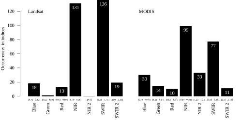
Figure 14: Distribution of the frequencies of the spectral bands of the learned indices for forest/savanna discrimination.

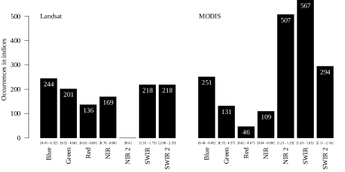
Figure 15: Distribution of the frequencies of the spectral bands of the learned indices for evergreen forest/semi-deciduous forest discrimination.

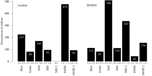
Figure 16: Distribution of the frequencies of the spectral bands of the learned indices for typical savanna/forested savanna discrimination.

The NIR2 and SWIR bands for the MODIS sensor have clear relevance in the evergreen forest/semi-deciduous forest problem, while, for Landsat, it is not prominent (Figure 15). The only agreement between the sensors is that the Red and NIR bands, which are used in the baselines, are the least frequent. The performance of GPVI for MODIS is about $11\%$ superior to Landsat (Table 4), which suggests that the NIR2 band has high relevance in characterizing these classes.

The typical savanna/forested savanna problem presented no agreement between the sensors (Figure 16). For example, the SWIR band is the most frequent for Landsat and the least frequent for MODIS, and the Red band, the most frequent for MODIS, is not so frequent for Landsat. This was also the most difficult pair of classes to discriminate in previous analyses.

Subexpression Relevance

Table 9 shows the top-ten most frequent formula elements found in the indices for the three classification problems.

Table 9: List of the most frequent formula elements for the three classification problems.

forest/savanna
Landsat
SWIR	NIR	-	%	rlog	srt	NIR%SWIR	*	+	rlog(NIR%SWIR)
136	131	127	120	104	92	83	55	29	22
MODIS
NIR	%	+	SWIR	-	srt	NIR2	*	NIR%SWIR	Blue
99	96	85	77	63	58	33	33	32	30
forest/semi-deciduous forest
Landsat
%	*	-	rlog	+	srt	Blue	SWIR	SWIR2	Green
444	344	336	261	249	245	244	218	218	201
MODIS
-	SWIR	%	NIR2	+	*	srt	SWIR2	Blue	rlog
622	470	436	425	356	279	276	224	189	181
typical savanna/forested savanna
Landsat
rlog	SWIR	%	*	srt	+	-	Blue	Red	NIR
551	476	401	353	335	291	246	223	167	95
MODIS
srt	Red	*	%	+	-	NIR2	rlog	srt(Red)	SWIR2
628	431	343	333	324	283	252	191	151	143

Regarding the Landsat data, it can be seen that the most recurrent bands are NIR and SWIR, and that the operations SWIR–NIR and SWIR2 % NIR appear various times. The following is an example of a GPVI learned in the forest/savanna classification problem for Landsat.

srt(Blue * rlog(SWIR - (NIR * SWIR2 - (SWIR - NIR)))) - ((NIR - (SWIR - (srt((srt((SWIR - (Blue * SWIR2 - (SWIR - NIR))) * Red) * rlog(rlog(rlog(srt(rlog(NIR) * ((Red * ((NIR - (rlog(rlog(Blue * SWIR2 - (SWIR2 % NIR - ((SWIR - (srt(SWIR) - Blue * SWIR2)) * rlog(SWIR2 % NIR))))) - Blue)) * Red)) - (SWIR - (Blue * SWIR2 - (SWIR - NIR))))))))) * rlog(SWIR2 % NIR)) - ((NIR - (SWIR - NIR)) % srt(SWIR))))) % srt(SWIR))

For MODIS, the NIR and SWIR bands are also the most recurrent, and the operations NIR2 % NIR and NIR % SWIR appear various times. The following is an example of a GPVI learned in the forest/savanna classification problem for MODIS.

srt(srt(NIR2 % NIR)) % ((NIR2 - srt(Green - (Green - (NIR2 + SWIR + (((Green % SWIR2) * (NIR % (NIR2 % NIR))) * (((((NIR % SWIR + 2 * Blue) * rlog(Red % NIR)) - (srt(srt(NIR % SWIR)) + 2 * Blue)) - (((NIR2 % NIR) * (Red % NIR)) * SWIR)) * ((((NIR % (NIR2 % NIR)) % SWIR) + Blue) + Blue))))))) - (NIR % SWIR + 2 * Blue))

For the classification of different physiognomies within the same biome, the complexity of the learned indices increases significantly, and a greater quantity of operations and constants appear in the formulas.

5 Discussion

The discussion about the results presented in Section 4 is guided by the research questions defined in Section 1. The performance of GPVI on the non-temporal-pixelwise forest/savanna classification problem (Q1) show a clear superiority of GPVI over NDVI, EVI, and EVI2. This suggests that there exist complex interactions between the bands that characterize the class of a sample, regardless of its behavior through time. In the baselines, savannas sometimes took high values that could be interpreted by the classification routine as forests, and vice versa (Figures 8 and 9). Thus, it is not possible to point out one area in a specific timestamp, measure its index, and conclude its class. For this reason, the traditional classification benchmark generally involves temporal information.

The relatively lower performance in the finer-scale classification problems, such as evergreen vs. semi-deciduous forest, and typical savanna vs. forested savanna (Q2), probably responds to both technical and biological factors. Firstly, the amount of data available for each physiognomical subcategory is significantly lower than for the biome classification problem (approximately half), and the amount of data for each class is unbalanced, due to the predominance of evergreen forests over semi-deciduous forests, and typical savannas over forested savannas in the study region. Those two factors are disadvantageous for most of the prediction tasks. However, discrimination by physiognomy within the same broader-scale biome type is, by itself, clearly a more complex biological problem. Moreover, while species composition could also be used to distinguish between these vegetation types, and different species can present different spectral signatures Alberton et al. (2014); Almeida et al. (2014), species composition can substantially overlap among the vegetation types considered here Leandro et al. (2018). All of these factors could have contributed to the limited results that were obtained for these specific classification problems.

Unlike single-pixel classification, the time series classification approach showed that the accuracy of GPVI was not significantly superior to the baselines (Q3). The most relevant reason is the fact that GPVI was originally trained for pixel classification, and the fitness function used drives the convergence of the algorithm to indices that minimize intra-class variance. This is clear and can be seen in Figures 8 and 9, in which the GPVI series are not only better separated, but also presented less variability through time. Part of the discriminative information in time series is, precisely, this variation, and the classification algorithm, which is based on DTW distance, took advantage of this variability in order to align/correct the series.

The experiments we conducted regarding sensor invariance, which was orthogonal to all of the experiments involving the Tropical South America regions, showed a consensus between Landsat and MODIS about the relevance of the bands for biome classification (Q4). Despite the sensor used, the most relevant channels are NIR and SWIR, which map, respectively, biomass content and soil moisture. This contrasts with indices traditionally used in vegetation studies in which the red channel has a leading role, meaning that, besides leaf reflectance (mapped by the NIR channel), soil moisture is more relevant to discriminate these types of biomes, rather than vegetation slope. A plausible explanation for this is that a closed canopy, as observed in forests, reduces light incidence and prevents soil water losses, reducing evapotranspiration and allowing for more water to be retained in the soil.

There was no consensus between the two sensors regarding the relevance of the bands for discriminating vegetation types within biomes. However, before concluding that these problems are unsolvable for spectral indices, factors, like the reduced quantity of data for training, the relatively low spectral resolution of the sensor, or the fact that MODIS includes noisy bands due to their low spatial resolution, must be considered. It is also important to notice that, unlike the forest/savanna problem, the experiments in MODIS sensor attributed a high relevance to channel NIR 2 (which is not provided by the Landsat sensor) when discriminating vegetation types. In both cases—evergreen forest vs. semi-deciduous forest and typical savanna vs. forested savanna—this channel was selected as the second most relevant. The fact that this channel is not provided by one of the sensors probably affected the consensus between the two. However, this area of the spectrum is not recognized as relevant for land-cover analysis in other studies and it is rather used to determine cirrus cloud contamination. Thus, no sound and straightforward interpretation could be made in these results alone. Nevertheless, we speculate that this result could be related to the role of forest in climate regulation given that forests can increase cloud formation above them Zemp et al. (2017).

6 Conclusions and Future Work

We introduced a Genetic-Programming-based framework for learning specialized vegetation indices from data, and tested it for discriminating between tropical South American forests and savannas, as well as the vegetation types existing within them. The framework outputs an index, which we called GPVI, optimized to project the spectral data of each pixel into a space where they can be easily discriminated. In the case of pixel-level discrimination, GPVI, when applied on each multispectral pixel to project them into a one-dimensional space, outperformed traditional indices, such as NDVI, EVI, and EVI2, showing that it is possible to describe discriminative patterns of the land coverage, without the use of entire time-series. Based on the same GPVI training procedure, we also tested the index for time-series classification and obtained a performance equivalent to baseline indices, despite the fact that the index was designed for single time stamp discrimination. Our index also outperformed traditional ones at discriminating between vegetation types within biomes, despite the high complexity involved in this specific problem. We speculate that the GPVI performance for this task could be highly improved with larger data availability and higher spectral resolution. When considering that biomes and vegetation types within biomes are dynamic and they can be replaced by one another over time in response to natural and anthropogenic disturbances, our approach is a promising framework for understanding how biomes will respond to present and future human induced global change drivers.

Our GP framework is also effective on hyperspectral data, with no further changes on its configuration. Experiments supporting this claim have already been published Hernández et al. (2016, 2017), in which the GP framework was tested on hyperspectral multi-class datasets, which not only contain vegetation areas, but also other types of land cover categories, and consider more than two classes. This demonstrates the robustness of our method with respect to the number and variety of bands, implying that GP is an approach that can naturally select and combine bands, regardless of heterogeneous setups, such as spatial/spectral resolution, type of land cover, and number of classes.

As future work, one promising approach can be to explicitly express the GP framework as multi-objective, as has been done in previous works Nag and Pal (2016); Liddle et al. (2010); Bleuler et al. (2001); Shao et al. (2013); Rodriguez-Vazquez et al. (2004); Tay and Ho (2008); Liang et al. (2019); this way, the relative importance between inter-class and intra-class distance of the examples can also be optimized, and novel objectives (e.g., precision and recall) can be considered.

Conceptualization, J.F.H.A. and R.d.S.T.; methodology, J.F.H.A. and R.d.S.T.; software, J.F.H.A.; validation, R.S.O., M.H. and J.A.d.S.; formal analysis, J.F.H.A.; investigation, J.F.H.A. and R.d.S.T.; resources, R.S.O. and M.H.; data curation, J.F.H.A.; writing—original draft preparation, J.F.H.A. and R.d.S.T.; writing—review and editing, R.S.O., M.H. and J.A.d.S.; visualization, J.F.H.A.; supervision, R.d.S.T.; project administration, R.d.S.T.; funding acquisition, R.d.S.T. All authors have read and agreed to the published version of the manuscript.

This research was funded by the Coordenação de Aperfeiçoamento de Pessoal de Nível Superior—Brasil (CAPES), grant #88881.145912/2017-01—Finance Code 001, Conselho Nacional de Desenvolvimento Científico e Tecnológico (CNPq), grants #307560/2016-3 and #132847/2015-9, Fundação de Amparo à Pesquisa do Estado de São Paulo (FAPESP) (grants #2018/06918-3, #2017/12646-3, #2016/26170-8, and #2014/12236-1) and the FAPESP-Microsoft Virtual Institute (grants #2016/08085-3, #2015/02105-0, #2014/50715-9, #2013/50169-1, and #2013/50155-0).