Two-Stage Training of Graph Neural Networks for Graph Classification

Abstract

Graph neural networks (GNNs) have received massive attention in the field of machine learning on graphs. Inspired by the success of neural networks, a line of research has been conducted to train GNNs to deal with various tasks, such as node classification, graph classification, and link prediction. In this work, our task of interest is graph classification. Several GNN models have been proposed and shown great accuracy in this task. However, the question is whether usual training methods fully realize the capacity of the GNN models. In this work, we propose a two-stage training framework based on triplet loss. In the first stage, GNN is trained to map each graph to a Euclidean-space vector so that graphs of the same class are close while those of different classes are mapped far apart. Once graphs are well-separated based on labels, a classifier is trained to distinguish between different classes. This method is generic in the sense that it is compatible with any GNN model. By adapting five GNN models to our method, we demonstrate the consistent improvement in accuracy and utilization of each GNN’s allocated capacity over the original training method of each model up to $5.4\%$ points in 12 datasets.

1 Introduction

With the pervasiveness of graph-structured data, graph representation learning has become an important task. Its goal is to learn embeddings (i.e., vector representations) of nodes and/or (sub)graphs. These embeddings are used in various downstream tasks, such as node classification, link prediction, and graph classification.

Metric learning is about learning distance between objects in a metric space. While it remains a difficult task to properly define an effective metric measure directly based on graph topology, a common approach is to map the graphs into vectors in the Euclidean space and measure the distance between those vectors. In addition to satisfying the basic properties of metrics, this mapping is also expected to separate graphs of different classes to distinguishable clusters.

Graph neural networks (GNNs) have received a lot of attention in the graph mining literature. Despite the challenge of applying the message-passing mechanism of neural networks to the graph structure, GNNs have proved successful in dealing with graph learning problems, including node classification  [27, 12], link prediction [24] and graph classification [31, 4, 6]. The common approach is to start from node features, allow information to flow among neighboring nodes and finalize the meaningful node embeddings. GNN models differ by the information-passing method and the objectives of the final embeddings.

Graph classification involves separating graph instances of different classes and predicting the label of an unknown graph. This task requires a graph representation vector distinctive enough to distinguish graphs of different classes. The subtlety is how to combine the node embeddings into an expressive graph representation vector, and a number of approaches have been proposed.

Although GNNs are shown to achieve high accuracy of graph classification, we observe that, with usual end-to-end training methods, they cannot realize their full potential. Thus, we propose 2STG+, a new training method with two stages. The first stage is metric learning with triplet loss, and the second stage is training a classifier. We observed that 2STG+ significantly improves the accuracy of five different GNN models, compared to their original training methods.

Our training method is, to some extent, similar to [10] and [18] in the sense that GNNs are pre-trained on a task before being used for graph classification. However, Hu et al. [10] does transfer learning by pre-training GNNs on a different massive graph, either in chemistry or biology domain, with numerous tasks, on both node and graph levels. Lu et al. [18] proposed the enhancement of pre-training steps by simulating the fine-tuning process of down-stream tasks to help the model adapt to future tasks. On the other hand, 2STG+ pre-trains GNNs on the same training dataset with only one graph-level task as the first stage. As highlighted in Table 1, 2STG+ is faster without requiring pre-training on rich and massive datasets, and it consistently achieves improved accuracy of more GNN models in more datasets than [10] and [18].

In short, the contributions of our paper are three-fold.

• Observation: In the graph classification task, GNNs often fail to exhibit their full power. Using a proper training method, their expressiveness can be further utilized.

• Method Design: We propose a two-stage learning method with pre-training based on triplet loss. With this method, up to 5.4% points in accuracy can be increased. Moreover, our method also utilizes the capacity of each GNN better by producing embeddings with higher intrinsic dimension and weaker correlation between embedding dimensions.

• Extensive Experiments: We conducted comprehensive experiments with 5 different GNN models and 12 datasets to illustrate the consistent improvement in accuracy and capacity utilization by our two-stage training method. We also compare our method with two strong graph transfer-learning methods to highlight the competency of our method.

Table 1: Comparison of our method 2STG+ with [10] and [18]. While they all need a pre-training step before graph classification, our method consistently improves accuracy of several GNNs even in datasets of a far domain while requiring shorter training time and no additional rich dataset.

	2STG+ (Proposed)	Transfer Learning [10]	L2P-GNN [18]
Accuracy improvement	5 out of 5 GNNs	3 out of 4 GNNs	4 out of 4 GNNs
	All datasets	Only within domain	Only within domain
Required datasets	No additional set	Large ($\approx$ 400K graphs)	Large ($\approx$ 400K graphs)
Total training time	Short ($\approx$ 1 hour)	Long ($\approx$ 1 day)	Long (several hours)

The rest of this paper is organized as follows. In Section 2, we review some relevant studies. In Section 3, we define the problem and describe our method. The experiments and results are presented in Section 4. We conclude our work in Section 5.

2 Related work

2.1 Graph neural networks

Graph neural networks (GNNs) attempt to learn embeddings (i.e, vector representations) of nodes and/or graphs, utilizing the mechanisms of neural networks adapted to the topology of graphs. The core idea of GNNs is to allow messages to pass between neighbors so that the representation of each node can incorporate the information from its neighborhood and thus to enable the GNNs to indirectly learn the graph structures. Numerous novel architectures for GNNs have been proposed and tested, which differ by the information-passing mechanisms. Among the most recent architectures are graph convolutions [12], attention mechanisms [27], and those inspired by convolutional neural networks [7, 21, 5]. The final embeddings obtained from GNNs can be utilized for various graph mining tasks, such as node classification [12], link prediction [24, 11], graph classification [31, 4], and influence maximization [13]. In addition, GNNs have been applied to some real-time tasks in computer vision, including but not limited to object detection [26], learning human-object interactions [23], and region classification [29].

2.2 Graph classification by GNNs

In graph classification, GNNs are tasked with predicting the label of an unseen graph. While node embeddings can be updated within a graph, the elusive step here is how to combine them into a vector representation of the entire graph that can distinguish among different labels. Two of the most common approaches are global pooling [6] and hierarchical pooling [30, 19, 15]. The simplest ways for global pooling are global entrywise mean and global entrywise max of the final node embeddings. In contrast, hierarchical pooling iteratively reduces the number of nodes either by merging similar nodes into supernodes [30, 19] or selecting the most significant nodes [15] until reaching a final supernode whose embedding is used to represent the whole graph.

2.3 Transfer learning for graphs

While most existing methods attempt to train GNNs as an end-to-end classification system, some studies considered transfer learning in which the GNN is trained on a large dataset before being applied to the task of interest, often in a much smaller dataset. Hu et al. [10] succeeded in improving 3 (out of 4 attempted) existing GNNs by transfer learning from other tasks. Rather than training a GNN to classify a dataset right away, the authors pre-trained that GNN on another massive dataset (up to 456K graphs); then they added a classifier and trained the whole architecture on the graph classification task. Lu et al. [18] also proposed a model consisting of two steps: pre-training and fine-tuning on downstream tasks. The key difference from  [10] is that the model learns to adapt by simulating the fine-tuning process during the pre-training step. However, transfer learning for graph remains a major challenge, as Ching et al. [3] and Wang et al. [28] pointed out, considerable domain knowledge is needed to design the appropriate pre-training procedure.

2.4 Metric learning

Metric learning aims to approximate a real-valued distance between two objects, and the most common objectives are contrastive loss and triplet loss. Some work has focused on metric learning on graphs [14, 17, 16]. Ktena et al. [14] and Liu et al. [17] employ a Siamese network structure, in which a twin network sharing the same weights is applied on a pair of graphs, and the two output vectors acting as representation of the two graphs are passed through a distance measure.

In computer vision, Schroff et al. [25] and Chechik et al. [1] learn metric on triplet of images, where two (anchor and positive) share the same label and one (negative) has a different label. The model aims to minimize the distance between the anchor and the positive, while maximizing the distance between the anchor and the negative. This inspired our interest in learning graph metrics with a triplet loss.

3 Proposed method

In this section, we first define our task of interest: graph classification. We then describe each component of our proposed training method of GNNs for graph classification.

Problem definition.

We tackle the task of graph classification. Given $\mathcal{D}=\{(G_{1},y_{1}),(G_{2},y_{2}),...\}$ where $y_{i}\in\mathcal{Y}$ is the class label of the graph $G_{i}\in\mathcal{G}$, the goal of graph classification is to learn a mapping $f:\mathcal{G}\to\mathcal{Y}$ that maps graphs to the set of class labels and predicts the class labels of unknown graphs.

Outline of our method.

Our method combines the advantages of both GNN and metric learning. Specifically, to facilitate a better accuracy of the classifier, our method first maps input graphs into vectors in the Euclidean space such that their corresponding vectors are well-separated based on classes. Below, we first briefly introduce GNNs and a learning scheme on triplet loss. We then describe the two stages of our method: pre-training a GNN and training a classifier.

3.1 Graph neural networks

Various GNNs have been proposed and proven effective in approximating such a function $f$. Starting from a graph $G=(V,E)$ with node features $X_{G}=\{\bm{x_{v}}|v\in V\}$, GNNs obtain final embeddings of nodes $Z_{G}=\{\bm{z_{v}}|v\in V\}$ and a final embedding $h_{G}$ of the graph after $K$ layers of aggregation. Specifically, at each $(k+1)$-th layer, the embedding $h_{v}^{(k+1)}$ of each node $v$ incorporates the embeddings of itself and its neighboring nodes $N(v)$ at the $k$-th layer as follows:

$$\bm{h_{v}^{(k+1)}}=MERGE\Big{(}\bm{h_{v}^{(k)}},AGGR\Big{(}\{\bm{h_{u}^{(k)}}|u\in N(v)\}\Big{)}\Big{)}$$

The embedding $h_{G}$ of the graph $G$ is then obtained by pooling all node embeddings into a single vector as follows:

$$\bm{h_{G}}=POOL\Big{(}\{\bm{h_{v}^{(i)}}|v\in V;i=1,..,K\}\Big{)}$$

GNNs differ by how the incorporating function $MERGE$, the aggregating function $AGGR$, and the final pooling function $POOL$ are implemented.

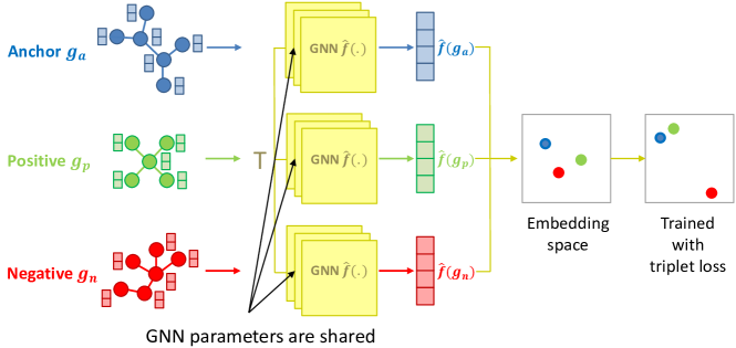
Figure 1: The first training stage for a GNN. $\hat{f}(.)$ is trained to differentiate graphs of different classes via the triplet loss.

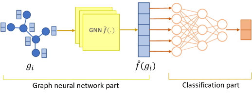
Figure 2: The second training stage for a classifier. After $\hat{f}(.)$ maps $g_{i}$ to $\bm{\hat{f}(g_{i})}$, a classifier is added to map $\bm{\hat{f}(g_{i})}$ to the class probability prediction. At this step, either the classifier is trained independently (2STG) or the whole architecture is trained together (2STG+).

3.2 Metric learning based on triplet loss

Triplet loss has been used for the learning of image similarity [25, 1]. The core idea is to enforce a margin between classes of samples. This results in embeddings of the same class mapped to a cluster distant apart from that of other classes. Specifically, given a mapping $\bar{f}$, we wish for a graph $g_{a}$ (anchor) to be closer to another graph $g_{p}$ (positive) of the same class than to a graph $g_{n}$ (negative) of another class by at least a margin $\alpha$, which is a hyperparameter:

$$\|\bm{\bar{f}(g_{a})}-\bm{\bar{f}(g_{p})}\|_{2}^{2}+\alpha<\|\bm{\bar{f}(g_{a})}-\bm{\bar{f}(g_{n})}\|_{2}^{2}.$$

The triplet loss for the whole dataset becomes:

$$\sum_{(a,p,n)}\max\left(\|\bm{\bar{f}(g_{a})}-\bm{\bar{f}(g_{p})}\|_{2}^{2}-\|\bm{\bar{f}(g_{a})}-\bm{\bar{f}(g_{n})}\|_{2}^{2}+\alpha,0\right)$$

with the summation over all considered triplets.

Our two-stage method combines the power of both GNNs and the metric learning method, as described below.

3.3 First training stage (pre-training a GNN)

In the first training stage (depicted in Fig. 1), given a GNN architecture $\hat{f}(.)$, its weights are shared among a triplet network $T$, which consists of three identical GNN architectures having the same weights as $\hat{f}(.)$. The parameters of $T$ are trained on each triplet of graphs $(g_{a},g_{p},g_{n})$ (anchor, positive, negative), in which the anchor and the positive graphs are of the same class while the negative graph is of another class. $T$ maps a triplet of graphs to a triplet of vectors in the Euclidean space: $T(g_{a},g_{p},g_{n})=(\bm{\hat{f}(g_{a})},\bm{\hat{f}(g_{p})},\bm{\hat{f}(g_{n})})$. Ideally, $\bm{\hat{f}(g_{a})}$ and $\bm{\hat{f}(g_{p})}$ should be close while $\bm{\hat{f}(g_{n})}$ is far from them both. The triplet loss for $(g_{a},g_{p},g_{n})$ is defined as:

$$\max\left(\|\bm{\hat{f}(g_{a})}-\bm{\hat{f}(g_{p})}\|_{2}^{2}-\|\bm{\hat{f}(g_{a})}-\bm{\hat{f}(g_{n})}\|_{2}^{2}+\alpha,0\right)$$

3.4 Second training stage (training a classifier)

In the second stage, a classifier is either trained independently, or added on top of the trained GNN and trained together on the graph classification task (see Fig. 2).

In summary, we propose two training methods for GNNs: 2STG and 2STG+, both consist of two stages.

• 2STG (Pre-training Setting): In the first stage, the GNN maps each triplet of graphs to a triplet of Euclidean-space vectors, and the GNN is trained on triplet loss. In the second stage, a classifier is trained independently to classify the graph embeddings.

• 2STG+ (Fine-tuning setting): It has the same structure as 2STG except that in the second stage, the classifier is plugged on top of the trained GNN, and then the whole architecture is trained together in an end-to-end manner.

Note that our methods are compatible to any GNN model that maps each graph to a representation vector. As shown in the next section, when applied to this method, each GNN model outperformed itself in the original setting.

4 Experiments

In this section, we describe the details of our experiments.

4.1 Experimental settings

4.1.1 GNN architectures

In order to demonstrate that our two-stage training method helps realize a better performance of GNNs, for each GNN architecture, we compared the accuracy obtained in the original setting versus that from our method. The GNN architectures we considered in this work are:

• GraphSage [9]: This is often used as a strong baseline in graph classification. After obtaining node embeddings, global mean/max pooling is applied to combine all node embeddings into one graph embedding.

• GAT [27]: Instead of uniformly passing neighbor information into a node embedding, Veličković et al. [27] uses an attention mechanism for the importance of each neighbor node.

• DiffPool [30]: While using the same aggregation mechanism as in [9], Ying et al. [30] proposes a hierarchical approach to pool the node embeddings. Rather than a “flat-pooling” step at the end, DiffPool repeatedly merges nodes into “supernodes” until there is only one supernode whose embedding is treated as the graph embedding.

• EigenGCN [19]: Attempting to implement hierarchical pooling like Ying et al. [30], Ma et al. [19] formulates a different way to combine nodes and their respective embeddings making use of the eigenvectors of the Laplacian matrix.

• SAGPool [15]: Hierarchical graph pooling employing self-attention mechanisms.

In previous studies, these models were trained end-to-end, mapping each graph to a prediction of class probabilities. To further illustrate the competency of our method, we also compared it with a transfer-learning method [10].

4.1.2 Datasets

We tested our training method using 12 datasets. Some statistics of the datasets are summarized in Table. 2 and 3.

Table 2: Some statistics of the benchmark datasets considered in this paper.

	Dataset
	DD	MUTAG	MUTAG2	PTC-FM	PROTEINS	IMDB-B
# Graphs	1,168	188	4,337	349	1,113	1,000
Avg. # Nodes	268.71	17.93	29.76	14.11	39.05	19.77
Avg. # Edges	676.21	19.79	30.76	14.48	72.81	96.53
# Classes	2	2	2	2	2	2

Table 3: Some statistics of the New York City Taxi datasets.

	Dataset
	Jan. G.	Feb. G.	Mar. G.	Jan. Y.	Feb. Y.	Mar. Y.
# Graphs	744	648	744	744	648	744
Avg. # Nodes	174.25	175.28	174.43	203.04	199.28	207.24
Avg. # Edges	497.35	502.96	480.33	1865.66	1868.28	1967.59
# Classes	2	2	2	2	2	2

Benchmark datasets

These are the commonly tested binary-class datasets [20] for the graph classification task. We use protein datasets (DD, MUTAG, MUTAG2, PTC-FM, and PROTEINS) and a collaboration network dataset IMDB-B. In each protein dataset, a graph is a protein, and the task is to predict whether the protein is an enzyme. In IMDB-B, each graph is an ego-network of actor collaborations, and the task is to predict the genre of the collaboration is either Action or Romance.

New York City Taxi datasets

We extracted the taxi ridership data in 2019 from New York City (NYC) Taxi Commission. The areas in New York are represented as nodes, and each taxi trip is an edge connecting the source and destination nodes. All taxi trips in an 1-hour interval form a graph, and each dataset spans a month of taxi operations. We augmented the binary label for each graph as taxi trips in weekdays (Mon-Thu) vs. weekend (Fri-Sun). We considered two taxi operators (Yellow and Green) and processed data in January, February and March of 2019, making 6 datasets in total: Jan. G., Feb. G., Mar. G., Jan. Y., Feb. Y., and Mar. Y..

4.1.3 Experimental procedure

We tested the ability of each GNN architecture to classify graphs in the following settings:

• Original setting: The GNN with a final classifier outputs the estimated class probabilities, and the weights are updated by the cross-entropy loss with respect to the ground truth. We use the implementation provided by the authors. To enhance the capacity of the final classifier, we tune it by using up to three fully-connected layers and select the model based on validation sets.

• 2STG and 2STG+: See Section 3.

In addition, we compared our two-stage method with the transfer-learning methods in [10] and [18], which also claimed the effectiveness of a pre-training strategy. Out of the 5 GNN models investigated in our work, GraphSage and GAT were provided with trained weights by Hu et al. [10], and they were compared with GraphSage and GAT trained in 2STG+. We also pre-trained GraphSage and GAT following the procedure in [18] and then fine-tuned them on our graph classification task and compared against 2STG+.

Each dataset was randomly split into three sets: training (80%), validation (10%) and test (10%) sets. The reported results are the mean and standard deviation of test accuracy over five splits.

We initialized node features as learnable features that were optimized with GNN parameters during training. While input features are provided in some datasets, according to our preliminary study, using learnable features often led to better accuracy.

In 2STG and 2STG+, each graph was used as an anchor once in each iteration, while the positive and negative graphs were chosen randomly. While Schroff et al. [25] suggested the potential advantage of choosing “hard” triplets and “semi-hard” triplets, what we empirically found was that the two options did not improve the classification accuracy. We used multi-layer perceptron (MLP) as the classifier.

4.1.4 Hyperparameter search

For each GNN, the hyperparameters regarding the network architecture were tuned in the same search space for each of the three settings to ensure fairness: original, 2STG, and 2STG+. The search space for the dimensions of the input vector, hidden vector and output vector for all GNNs was $\{16,32,64,96,128\}$. For DiffPool, we used three layers of graph convolution and one DiffPool layer as described in the original paper. For EigenGCN, we used three pooling operators as it was shown to achieve the best performance in the original paper. For SAGPool, we used three pooling layers as explained in the original paper. Other hyperparameters that are exclusive to each GNN architecture were set to the default values provided in each paper’s original code of each architecture’s authors.

In each of the three settings, the architecture of the final classifier was also tuned in the same search space. The number of fully-connected layers was up to 3 while the search space for the hidden dimension was $\{2^{h}|1\leq h\leq\log_{2}(d)\}$, where $d$ is the dimension of the output vector. As shown in Appendix A, using a strong classifier is helpful in improving the classification accuracy.

The two settings 2STG and 2STG+ require an additional hyperparameter $\alpha$ as the margin in the triplet loss. While Schroff et al. [25] found $\alpha=0.2$ to be effective, we empirically found that this value was too small to separate instances of different classes. Instead, the search space for $\alpha$ we used was $\{0.5,1.0,1.5,2.0,2.5\}$. Grid search showed that the performance was sensitive with respect to the choice of $\alpha$.

4.1.5 Computing specifications & dependencies

All experiments were performed on Ubuntu 18.04 LTS running on a machine with 4 RTX-2080Ti GPUs, each of which has $11$GB memory. The following libraries were used to run the code: torch 1.7.0, networkx 2.5, sklearn 0.23.2, numpy 1.16.4, and torch-geometric 1.6.3.

4.2 Results and discussion

4.2.1 Improvement by our methods

We draw some observations from the results of comparing 2STG and 2STG+ with the original setting (Tables 4 and 5):

Table 4: Average and standard deviation (in %) of graph classification accuracies in benchmark datasets in three settings: original, 2STG, and 2STG+. Pre-training GNNs in 2STG improves the classification accuracy compared to the original setting, and fine-tuning GNNs in 2STG+ further improves the accuracy. The average gain is in % points.

Method	Dataset						Average Gain
	DD	MUTAG	MUTAG2	PTC-FM	PROTEINS	IMDB-B	(in % points)
GraphSage	69.24 $\pm$ 0.52	65.13 $\pm$ 0.87	75.44 $\pm$ 0.50	61.77 $\pm$ 1.11	71.25 $\pm$ 1.38	65.52 $\pm$ 0.96	-
GraphSage (2STG)	75.13 $\pm$ 0.82	80.86 $\pm$ 1.19	76.84 $\pm$ 0.54	62.75 $\pm$ 1.20	71.29 $\pm$ 0.41	68.37 $\pm$ 0.63	4.47
GraphSage (2STG+)	76.52 $\pm$ 1.47	81.14 $\pm$ 0.68	77.71 $\pm$ 0.41	62.65 $\pm$ 0.72	72.34 $\pm$ 0.56	68.24 $\pm$ 0.83	5.01
GAT	66.50 $\pm$ 1.24	65.18 $\pm$ 1.03	76.23 $\pm$ 0.67	60.65 $\pm$ 0.42	66.92 $\pm$ 0.75	67.13 $\pm$ 0.88	-
GAT (2STG)	72.95 $\pm$ 0.91	77.84 $\pm$ 0.63	76.34 $\pm$ 0.52	62.04 $\pm$ 1.16	70.17 $\pm$ 0.72	69.15 $\pm$ 0.87	4.11
GAT (2STG+)	74.13 $\pm$ 1.47	78.17 $\pm$ 1.41	76.49 $\pm$ 1.23	61.61 $\pm$ 0.53	72.64 $\pm$ 0.58	67.25 $\pm$ 0.89	5.37
DiffPool	72.11 $\pm$ 0.42	86.32 $\pm$ 0.83	77.21 $\pm$ 1.16	61.15 $\pm$ 0.35	72.24 $\pm$ 0.67	64.93 $\pm$ 0.74	-
DiffPool (2STG)	74.93 $\pm$ 0.53	86.14 $\pm$ 0.77	77.94 $\pm$ 1.28	62.03 $\pm$ 0.32	73.87 $\pm$ 0.64	65.22 $\pm$ 0.83	1.03
DiffPool (2STG+)	78.84 $\pm$ 0.54	87.38 $\pm$ 0.62	77.08 $\pm$ 1.23	62.15 $\pm$ 0.68	73.07 $\pm$ 1.17	64.90 $\pm$ 0.81	1.07
EigenGCN	75.62 $\pm$ 0.63	79.87 $\pm$ 0.66	76.65 $\pm$ 1.14	63.34 $\pm$ 1.23	75.63 $\pm$ 0.82	71.86 $\pm$ 0.55	-
EigenGCN (2STG)	77.56 $\pm$ 0.48	80.21 $\pm$ 0.71	77.98 $\pm$ 0.62	64.13 $\pm$ 0.95	75.93 $\pm$ 0.56	72.66 $\pm$ 0.42	0.91
EigenGCN (2STG+)	78.13 $\pm$ 0.51	81.42 $\pm$ 0.86	77.02 $\pm$ 1.72	63.52 $\pm$ 1.43	77.31 $\pm$ 1.46	72.04 $\pm$ 0.53	1.07
SAGPool	76.12 $\pm$ 0.79	78.34 $\pm$ 0.65	76.83 $\pm$ 1.27	63.27 $\pm$ 0.78	74.34 $\pm$ 1.25	71.23 $\pm$ 1.12	-
SAGPool (2STG)	78.32 $\pm$ 1.26	79.63 $\pm$ 0.95	78.03 $\pm$ 0.68	63.83 $\pm$ 0.83	77.52 $\pm$ 0.54	71.73 $\pm$ 0.81	1.48
SAGPool (2STG+)	78.22 $\pm$ 0.70	79.03 $\pm$ 0.89	77.03 $\pm$ 0.63	64.34 $\pm$ 0.86	76.23 $\pm$ 1.12	72.36 $\pm$ 0.73	1.24

• Pre-training using triplet loss (i.e., the first stage of 2STG and 2STG+) consistently enhances the graph classification accuracy of each GNN model by $0.9-5.4\%$ points, compared to its original setting.

• Fine-tuning the weights of GNNs (i.e, the second stage of 2STG+) further improves the accuracy from 2STG in some cases by up to 1.3% points.

Table 5: Average and standard deviation (in %) of graph classification accuracies in NYC Taxi datasets in three settings: original, 2STG, and 2STG+. Similarly to the case of the benchmark datasets, 2STG and 2STG+ significantly outperform the original setting. G., Y. stand for Green, Yellow. The average gain is in % points.

Method	Dataset						Average Gain
	Jan. G.	Feb. G.	Mar. G.	Jan. Y.	Feb. Y.	Mar. Y.	(in % points)
GraphSage	73.14 $\pm$ 0.62	66.35 $\pm$ 1.25	64.63 $\pm$ 0.83	72.86 $\pm$ 0.92	64.37 $\pm$ 0.87	68.12 $\pm$ 0.76	-
GraphSage (2STG)	76.14 $\pm$ 0.93	66.67 $\pm$ 1.31	67.13 $\pm$ 0.85	75.24 $\pm$ 1.16	65.43 $\pm$ 0.68	70.15 $\pm$ 0.64	1.88
GraphSage (2STG+)	76.63 $\pm$ 0.82	67.74 $\pm$ 0.88	68.95 $\pm$ 1.41	75.21 $\pm$ 1.70	67.64 $\pm$ 0.73	70.23 $\pm$ 1.25	2.82
GAT	71.26 $\pm$ 1.51	67.82 $\pm$ 0.77	66.13 $\pm$ 0.72	72.64 $\pm$ 0.54	64.76 $\pm$ 0.73	67.51 $\pm$ 1.69	-
GAT (2STG)	75.23 $\pm$ 0.82	67.24 $\pm$ 0.56	67.34 $\pm$ 0.71	76.82 $\pm$ 1.23	66.45 $\pm$ 0.85	70.66 $\pm$ 0.78	2.27
GAT (2STG+)	74.65 $\pm$ 0.98	68.11 $\pm$ 0.69	69.15 $\pm$ 1.37	74.79 $\pm$ 1.27	68.75 $\pm$ 0.66	70.44 $\pm$ 0.93	3.04
DiffPool	78.43 $\pm$ 0.74	73.12 $\pm$ 0.42	71.39 $\pm$ 1.56	72.52 $\pm$ 1.23	67.43 $\pm$ 0.87	74.34 $\pm$ 0.77	-
DiffPool (2STG)	80.28 $\pm$ 1.16	75.69 $\pm$ 1.21	73.79 $\pm$ 0.81	75.09 $\pm$ 0.72	68.19 $\pm$ 0.50	74.87 $\pm$ 0.83	1.78
DiffPool (2STG+)	79.63 $\pm$ 0.82	74.56 $\pm$ 1.32	72.92 $\pm$ 0.65	75.95 $\pm$ 1.21	69.31 $\pm$ 0.97	75.76 $\pm$ 0.86	1.81
EigenGCN	75.45 $\pm$ 0.44	69.32 $\pm$ 1.82	72.21 $\pm$ 0.83	73.21 $\pm$ 1.35	69.64 $\pm$ 0.76	69.52 $\pm$ 1.54	-
EigenGCN (2STG)	77.14 $\pm$ 0.81	70.03 $\pm$ 0.62	74.12 $\pm$ 1.34	74.36 $\pm$ 1.65	69.72 $\pm$ 0.97	70.03 $\pm$ 0.86	1.02
EigenGCN (2STG+)	76.73 $\pm$ 1.21	71.27 $\pm$ 1.33	73.37 $\pm$ 1.85	75.33 $\pm$ 1.14	71.65 $\pm$ 1.67	71.84 $\pm$ 0.62	1.80
SAGPool	73.23 $\pm$ 0.59	67.46 $\pm$ 0.73	72.78 $\pm$ 1.34	72.65 $\pm$ 0.72	68.83 $\pm$ 1.25	69.68 $\pm$ 1.35	-
SAGPool (2STG)	76.36 $\pm$ 1.37	69.07 $\pm$ 1.48	74.34 $\pm$ 1.52	71.11 $\pm$ 0.73	70.02 $\pm$ 0.64	70.04 $\pm$ 1.48	1.05
SAGPool (2STG+)	75.38 $\pm$ 0.86	69.27 $\pm$ 1.12	73.19 $\pm$ 1.34	72.51 $\pm$ 0.85	69.16 $\pm$ 0.79	70.59 $\pm$ 0.52	0.91

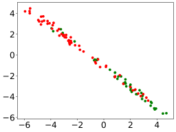
(a) Original

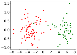
(b) 2STG

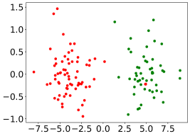
(c) 2STG+

Figure 3: Visualization of the final embeddings in Original (left), 2STG (middle) and 2STG+ (right) settings (DD dataset). Instances of the two classes are separated better in 2STG and 2STG+ than in the original setting.

DD Dataset:

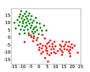
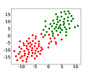
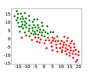
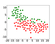
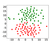
Feb. G. dataset:

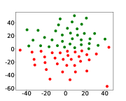
(a) GraphSage

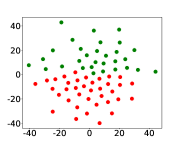
(b) GAT

(c) DiffPool

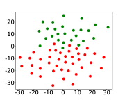
(d) EigenGCN

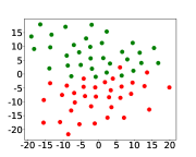
(e) SAGPool

Figure 4: Visualization of the graph embeddings after training with the triplet loss in the DD (top) and Feb. G. (bottom) datasets. T-SNE is applied to reduce the embedding dimension from 64 to 2 for visualization. Two colors represent two classes. Training with the triplet loss separates most instances of the two classes.

The improvement in accuracy by 2STG and 2STG+ suggests two explanations:

• The end-to-end training methods fail to realize the full potential of the GNN models. Even if the final classifier is upgraded from a fully-connected layer to an MLP, the accuracy is not as high as in 2STG and 2STG+.

• Learning meaningful embeddings in between that are fairly separated based on classes (see Figures 3 and 4), for example through metric learning as in our methods, facilitates a better accuracy of the final classifier.

4.2.2 Comparison with a transfer learning method

We compared the pre-trained models of GraphSage and GAT in [10] and [18] with GraphSage and GAT trained in 2STG+. Specifically, we obtained the weights of GraphSage and GAT pretrained in [10], and they are referred to as GraphSage (Tf) and GAT (Tf). We pre-trained GraphSage and GAT with the same architecture (i.e., $5$ layers, $300$ dimensional hidden units, and global mean pooling) by the code provided in [18] and denoted them as GraphSage (L2P) and GAT (L2P). We also pretrained GraphSage and GAT with the same architecture according to the first training stage (see Section 3.3), and they are referred to as GraphSage (2STG+) and GAT (2STG+). They were trained with different values of the margin hyperparameter $\alpha$ as specified in Section 4.1.4. In the classifier training step, GraphSage (Tf), GAT (Tf), GraphSage (L2P), GAT (L2P), GraphSage (2STG+), and GAT (2STG+) were fine-tuned according to the second training stage (see Section 3.4) with the same search space of the architecture of the final classifier as specified in Section 4.1.4. The other settings were the same as those described in Section 4.1.3.

Table 6: 2STG+ outperforms the two transfer learning methods (Tf [10] and L2P [18]) in terms of classification accuracy in most cases when the benchmark datasets are used. Note that 2STG+ has several advantages over the transfer learning methods, as highlighted in Table 1. The last column shows how much higher the average accuracy of 2STG is than that of Tf and L2P.

Method	Dataset						Average Gap
	DD	MUTAG	MUTAG2	PTC-FM	PROTEINS	IMDB-B	(in % points)
GAT (2STG+)	74.11 $\pm$ 1.42	78.09 $\pm$ 1.25	76.62 $\pm$ 1.37	61.56 $\pm$ 0.59	72.67 $\pm$ 0.67	67.27 $\pm$ 0.81	-
GAT (Tf)	72.24 $\pm$ 0.83	76.86 $\pm$ 1.35	75.59 $\pm$ 1.48	61.28 $\pm$ 0.97	71.76 $\pm$ 0.77	65.16 $\pm$ 1.47	1.56
GAT (L2P)	73.87 $\pm$ 0.95	75.98 $\pm$ 0.92	76.38 $\pm$ 1.25	60.73 $\pm$ 1.02	71.48 $\pm$ 0.93	66.59 $\pm$ 1.21	0.88
GraphSage (2STG+)	76.29 $\pm$ 1.25	81.12 $\pm$ 0.61	77.62 $\pm$ 0.47	62.87 $\pm$ 0.63	72.51 $\pm$ 0.59	68.18 $\pm$ 1.03	-
GraphSage (Tf)	75.26 $\pm$ 1.36	82.43 $\pm$ 1.49	76.83 $\pm$ 0.95	62.61 $\pm$ 0.78	72.15 $\pm$ 0.83	67.14 $\pm$ 0.52	0.31
GraphSage (L2P)	74.87 $\pm$ 1.13	81.56 $\pm$ 1.25	77.35 $\pm$ 0.64	61.13 $\pm$ 0.76	72.78 $\pm$ 0.69	68.03 $\pm$ 0.78	0.48

Table 7: 2STG+ leads to higher classification accuracy than the two transfer learning methods (Tf [10] and L2P [18]) in most NYC Taxi datasets. Compared with Table 6, the gap is larger as the GNNs for transfer learning were pre-trained on a biology dataset, which is of a far domain. The last column shows how much higher the average accuracy of 2STG is than that Tf and L2P.

Method	Dataset						Average Gap
	Jan.G.	Feb. G.	Mar. G.	Jan. Y.	Feb. Y.	Mar. Y.	(in % points)
GAT (2STG+)	74.47 $\pm$ 0.87	68.19 $\pm$ 0.57	69.19 $\pm$ 1.02	74.72 $\pm$ 1.23	68.81 $\pm$ 0.63	70.51 $\pm$ 0.93	-
GAT (Tf)	73.87 $\pm$ 1.13	65.89 $\pm$ 1.04	67.25 $\pm$ 1.27	71.87 $\pm$ 1.35	66.24 $\pm$ 0.92	68.95 $\pm$ 1.25	1.97
GAT (L2P)	73.36 $\pm$ 0.75	66.84 $\pm$ 0.97	67.91 $\pm$ 1.14	74.08 $\pm$ 1.16	67.59 $\pm$ 0.87	68.37 $\pm$ 0.98	1.29
GraphSage (2STG+)	76.41 $\pm$ 0.93	67.79 $\pm$ 0.82	69.02 $\pm$ 1.25	75.33 $\pm$ 1.48	67.61 $\pm$ 0.71	70.21 $\pm$ 1.32	-
GraphSage (Tf)	75.19 $\pm$ 0.98	67.82 $\pm$ 0.43	68.03 $\pm$ 0.66	73.66 $\pm$ 1.27	68.24 $\pm$ 0.79	70.25 $\pm$ 0.73	0.53
GraphSage (L2P)	75.04 $\pm$ 0.83	68.24 $\pm$ 0.76	68.37 $\pm$ 0.96	74.17 $\pm$ 1.16	67.08 $\pm$ 0.54	70.96 $\pm$ 0.82	0.42

As shown in Tables 6 and 7, despite being pre-trained on a much smaller dataset, 2STG+ achieves better accuracy in $83\%$ of the considered cases: up to $2\%$ points in the benchmark datasets and up to $3\%$ points in the NYC Taxi datasets. This validates our claims in Table 1.

4.2.3 Running time

For each hyperparameter setting in a dataset, the original setting takes up to half an hour to train a model. Due to having two stages, 2STG and 2STG+ take up to an hour for both stages. In [10], the transfer-learning method was reported to take up to one day to pre-train on a rich dataset. Pre-training each GNN architecture accordingly to [18] took several hours to complete.

4.3 Further analysis

We study the final embeddings, generated by three training methods: original, 2STG, 2STG+. In Fig. 3, despite having 2 dimensions, the embeddings of the original setting can be reduced to 1 dimension. We suspect that given the potential capacity, specifically the dimension of the final embeddings, 2STG and 2STG+ utilize such expressive power better than the original setting by resulting in higher intrinsic dimension, weaker correlation between dimensions, and larger distance between embeddings [2]. While measuring the distance did not provide clear evidence, the results of the other two measurements validate our hypothesis.

4.3.1 Intrinsic dimension

We measure the intrinsic dimension, which we define as the dimension needed to retain 99$\%$ of the variance in the final embeddings. In the final embeddings of dimension $d$ of the validation set, we apply Principal Component Analysis (PCA) and measure the cumulative explained variance $V(i)$ achieved by setting the final dimension as $i$ for $i=1,2,..,d$. Assume that $V(j)\leq 0.99\leq V(j+1)$, we linearly interpolate between $j$ and $(j+1)$ to obtain the dimension with $99\%$ explained variance. Such dimensions are reported in Tables 8 and 9. Given $64$ dimensions as the capacity, 2STG and 2STG+ retain a higher intrinsic dimension, implying that they utilize this capacity better than the original setting. As an illustrative example from the MUTAG dataset in Fig. 5 shows, most of the variance can be explained by lower dimensions in the original setting than in 2STG and 2STG+.

Table 8: Intrinsic dimension obtained by PCA on embeddings of dimension 64 for the benchmark datasets. Each entry is the mean of 5 runs. In most cases, the GNNs trained in 2STG and 2STG+ lead to higher intrinsic dimensions than that trained in the original setting.

Method	Dataset
	DD	MUTAG	MUTAG2	PTC-FM	PROTEINS	IMDB-B
GraphSage	37.01	9.03	10.23	8.76	33.67	24.41
GraphSage (2STG)	38.83	9.98	17.21	19.98	36.13	24.18
GraphSage (2STG+)	18.33	9.18	30.27	16.65	18.11	14.31
GAT	8.38	9.65	12.26	11.07	33.72	26.46
GAT (2STG)	34.53	10.88	20.47	18.73	31.13	15.33
GAT (2STG+)	31.17	9.37	18.54	16.94	33.88	14.54
DiffPool	6.69	3.69	15.97	13.17	14.33	14.31
DiffPool (2STG)	37.16	7.94	22.64	20.02	18.25	19.39
DiffPool (2STG+)	15.11	8.08	25.19	7.02	10.21	11.21
EigenGCN	14.76	4.98	20.49	12.57	17.94	17.21
EigenGCN (2STG)	25.63	8.71	31.53	19.77	19.26	17.32
EigenGCN (2STG+)	22.76	5.38	28.75	19.62	19.57	11.74
SAGPool	15.86	2.81	17.88	12.99	11.82	17.31
SAGPool (2STG)	29.46	9.76	18.25	15.67	16.83	18.49
SAGPool (2STG+)	25.83	7.31	18.37	14.74	15.87	11.75

Table 9: Intrinsic dimension obtained by PCA on embeddings of dimension 64 for the New York Taxi datasets. Each entry is the mean of 5 runs. In almost all cases, the embeddings obtained by the GNNs trained in 2STG and 2STG+ have higher intrinsic dimensions than those obtained by the GNNs trained in the original setting.

Method	Dataset
	Jan. G.	Feb. G.	Mar. G.	Jan. Y.	Feb. Y.	Mar. Y.
GraphSage	26.46	30.49	32.21	31.02	21.24	23.41
GraphSage (2STG)	35.98	36.03	36.98	38.95	38.61	36.64
GraphSage (2STG+)	37.56	33.37	29.88	24.06	23.51	32.07
GAT	35.17	34.44	33.61	32.01	36.95	31.72
GAT (2STG)	23.57	25.24	38.01	39.02	24.34	23.33
GAT (2STG+)	36.89	38.27	26.98	35.18	23.57	28.42
DiffPool	4.64	16.84	6.62	16.56	16.19	15.71
DiffPool (2STG)	33.03	32.77	26.78	36.01	33.09	33.93
DiffPool (2STG+)	32.57	33.14	26.22	30.93	20.84	30.35
EigenGCN	3.98	15.59	3.19	15.77	28.02	23.47
EigenGCN (2STG)	31.21	32.45	27.68	32.81	26.55	26.92
EigenGCN (2STG+)	32.26	33.98	18.87	30.87	31.01	26.47
SAGPool	5.42	17.66	3.75	14.99	25.09	20.01
SAGPool (2STG)	31.81	28.57	31.19	32.71	28.19	31.11
SAGPool (2STG+)	33.18	32.49	28.16	21.31	27.56	29.11

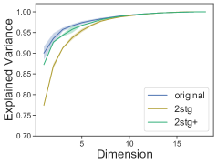
(a) GraphSage

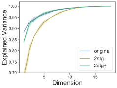
(b) GAT

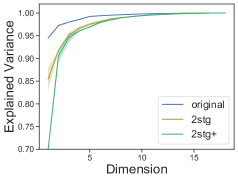
(c) DiffPool

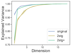
(d) EigenGCN

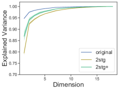
(e) SAGPool

Figure 5: Explained variance with respect to dimensions when applying PCA to the embeddings generated by each GNN trained in the original setting, 2STG, and 2STG+ on the MUTAG dataset. Means and standard deviation of 5 runs are plotted. The respective intrinsic dimensions are reported in Table 8. In order to retain $99\%$ of the explained variance, the embeddings obtained in the original setting require lower dimensions than those obtained in 2STG and 2STG+.

4.3.2 Correlation between final embedding dimensions

We measure the average absolute correlation coefficients between final embedding dimensions. Specifically, given final embeddings of dimension five, the average of absolute values of ${5\choose 2}$ pairwise correlation coefficients is calculated. As seeen in Tables 10 and 11, in most of the cases, the original setting leads to stronger correlation than 2STG and 2STG+, and several obtained dimensions are too strongly correlated, making them redundant. This implies that 2STG and 2STG+ utilize the provided capacity (i.e., dimension of final embeddings) better than the original setting by giving fewer redundant dimensions. As seen in Fig. 6, the average absolute correlation coefficients in the original setting quickly become close to 1. In 2STG and 2STG+, such correlation is much weaker.

Table 10: Average absolute correlation coefficients between the five dimensions of the final embeddings for the benchmark datasets. Each entry is the mean of 5 runs, and it ranges from $0$ to $1$. Higher values indicate stronger correlation between the dimensions. In all cases, the original setting leads to stronger correlation between the dimensions than 2STG and 2STG+.

Method	Dataset
	DD	MUTAG	MUTAG2	PTC-FM	PROTEINS	IMDB-B
GraphSage	0.94	0.77	0.91	0.56	0.96	0.55
GraphSage (2STG)	0.67	0.66	0.26	0.28	0.43	0.31
GraphSage (2STG+)	0.62	0.59	0.42	0.45	0.41	0.32
GAT	0.92	0.98	0.87	0.62	0.82	0.84
GAT (2STG)	0.72	0.45	0.25	0.26	0.46	0.53
GAT (2STG+)	0.64	0.56	0.29	0.37	0.41	0.47
DiffPool	0.81	0.85	0.75	0.49	0.91	0.87
DiffPool (2STG)	0.36	0.52	0.51	0.35	0.38	0.39
DiffPool (2STG+)	0.32	0.44	0.47	0.31	0.42	0.33
EigenGCN	0.72	0.92	0.71	0.58	0.84	0.78
EigenGCN (2STG)	0.58	0.51	0.47	0.45	0.57	0.34
EigenGCN (2STG+)	0.54	0.75	0.42	0.37	0.43	0.32
SAGPool	0.75	0.98	0.62	0.47	0.82	0.82
SAGPool (2STG)	0.49	0.61	0.38	0.26	0.34	0.44
SAGPool (2STG+)	0.41	0.55	0.36	0.31	0.32	0.41

Table 11: Average absolute correlation coefficients between the five dimensions of the final embeddings for the New York Taxi datasets. Each entry is the mean of 5 runs, and it ranges from $0$ to $1$. Higher values indicate stronger correlation between the dimensions. In most cases, the original setting leads to stronger correlation between the dimensions than 2STG and 2STG+.

Method	Dataset
	Jan. G.	Feb. G.	Mar. G.	Jan. Y.	Feb. Y.	Mar. Y.
GraphSage	0.92	0.87	0.95	0.89	0.89	0.94
GraphSage (2STG)	0.41	0.66	0.66	0.68	0.61	0.84
GraphSage (2STG+)	0.45	0.76	0.66	0.62	0.54	0.49
GAT	0.71	0.77	0.91	0.86	0.78	0.86
GAT (2STG)	0.54	0.54	0.61	0.41	0.52	0.52
GAT (2STG+)	0.65	0.84	0.58	0.48	0.58	0.46
DiffPool	0.95	0.88	0.97	0.98	0.59	0.97
DiffPool (2STG)	0.66	0.51	0.61	0.76	0.83	0.88
DiffPool (2STG+)	0.57	0.92	0.59	0.44	0.39	0.53
EigenGCN	0.97	0.97	0.92	0.95	0.94	0.98
EigenGCN (2STG)	0.68	0.78	0.56	0.44	0.53	0.84
EigenGCN (2STG+)	0.45	0.71	0.51	0.44	0.48	0.63
SAGPool	0.99	0.94	0.88	0.73	0.93	0.92
SAGPool (2STG)	0.31	0.42	0.51	0.56	0.62	0.49
SAGPool (2STG+)	0.38	0.41	0.57	0.92	0.57	0.53

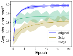
(a) GraphSage

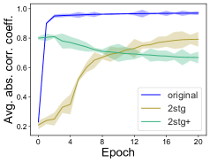
(b) GAT

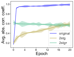
(c) DiffPool

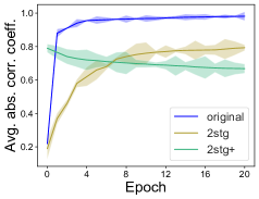
(d) EigenGCN

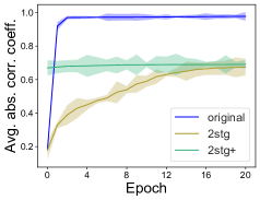
(e) SAGPool

Figure 6: Average absolute correlation coefficients over epochs on the Jan. G. dataset. Means and standard deviations of 15 runs are plotted. Embedding dimensions quickly become strongly correlated in the orginal setting. Such correlation is much weaker in 2STG and 2STG+.

5 Conclusion

Graph neural networks are powerful tools in dealing with the graph classification task. However, training them end-to-end to predict class probabilities often fails to realize their full capability. Thus, we apply GNN models in a triplet framework to learn discriminative embeddings first, and then train a classifier on those embeddings. Extensive experiments in 12 datasets lead to following observations:

• End-to-end training often fails to realize the full potential of GNN models. Our method consistently improves the accuracy of $5$ (out of $5$ tested) GNN models in $12$ (out of $12$ considered) datasets over the original setting.

• Despite not requiring any additional massive datasets or long training time, our two-stage method obtains better accuracy than a state-of-the-art pre-training method based on transfer-learning in 83% of the cases.

• Training each GNN in our method utilizes the given capacity better by producing embeddings with higher intrinsic dimension and weaker correlation between dimensions.

As future work, we would like to address some current limitations of our method and expand the scope of our work. One possible approach is to reduce the overhead in triplet sampling to reduce the overall training time by using fast nearest-neighbor search techniques (e.g., [22, 8]). We will also consider employing the global loss [14] or the Siamese Community-Preserving loss objective [17] instead of the triplet loss. In addition, we will apply the two-stage training idea to other downstream tasks, such as node classification and edge label prediction.

Availability of data and code

The source code and datasets used in the study are available at http://github.com/manhtuando97/two-stage-gnn.

Appendix A Appendix: Effect of Classification Layers

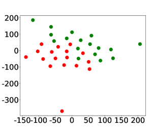
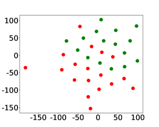
Jan. G. Dataset:

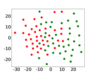
(a) 2STG+ with one classification layer

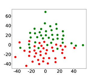
(b) 2STG+ with up to three classification layer

Figure 7: Graph embeddings generated by GraphSAGE for the datasets PTC-FM and JAN. G. in the two cases of 2STG+ with one classification layer (left) and 2STG+ with up to three classification layers (right), respectively. These are the graphs embeddings (i.e., $\hat{f}(g_{i})$ of each graph $g_{i}$), which are the input of the classification part in Fig. 2. T-SNE is applied to reduce the embedding dimension from 64 to 2 for visualization. Due to the capacity difference of the classifiers (one layer vs. up to three layers), there is a gap in the final classification accuracies of the two cases reported in Tables 12 and 13.

We report in Tables 12 and 13 the classification accuracy when the classifier only consists of one layer and when the classifier is tuned using up to three layers (as described in Section. 4.1.4). In some cases, the 1-layer classifier could achieve an accuracy that is close or slightly higher than that of the classifier using up to three layers. However, tuning the model using up to three classification layers allows us to achieve better accuracy than using only one layer for the classifier in most cases. The few exceptions are highlighted in red in Tables 12 and 13. These results indicate that using a strong classifier is generally helpful in enhancing the classification accuracy. We also visualize in Fig. 7 the cases in which the differences between using one classification layer and using up to three classification layers are the highest. In particular, we highlight the t-SNE visualization of the embeddings generated by GraphSage 2STG+ for the datasets PTC-FM and JAN. G. when using one classification layer and up to three classification layers, respectively.

Table 12: Classification accuracy when the classifier consists of one layer and when the classifier is tuned using up to three layers on the benchmark datasets. 2STG $=1$ and 2STG $\leq 3$ represent 2STG with one classification layer and up to three classification layers (as detailed in Section. 4.1.4), respectively. The same applies for 2STG+ $=1$ and 2STG+ $\leq 3$. In almost all cases, tuning the classifier using up to three classifier layers leads to better accuracy than using only one layer.

GNN	Method	Dataset
	(# Layers)	DD	MUTAG	MUTAG2	PTC-FM	PROTEINS	IMDB-B
GraphSage	2STG $=1$	74.92 $\pm$ 0.76	80.13 $\pm$ 1.07	75.63 $\pm$ 0.78	60.24 $\pm$ 1.13	69.87 $\pm$ 0.35	68.42 $\pm$ 0.45
	2STG $\leq 3$	75.13 $\pm$ 0.82	80.86 $\pm$ 1.19	76.84 $\pm$ 0.54	62.75 $\pm$ 1.20	71.29 $\pm$ 0.41	68.37 $\pm$ 0.63
	2STG+ $=1$	76.14 $\pm$ 1.33	80.97 $\pm$ 0.59	77.82 $\pm$ 0.56	60.13 $\pm$ 0.65	70.26 $\pm$ 0.53	68.17 $\pm$ 0.71
	2STG+ $\leq 3$	76.52 $\pm$ 1.47	81.14 $\pm$ 0.68	77.71 $\pm$ 0.41	62.65 $\pm$ 0.72	72.34 $\pm$ 0.56	68.24 $\pm$ 0.83
GAT	2STG $=1$	72.68 $\pm$ 0.84	76.13 $\pm$ 0.48	75.32 $\pm$ 0.54	60.86 $\pm$ 1.04	69.73 $\pm$ 0.58	68.97 $\pm$ 0.82
	2STG $\leq 3$	72.95 $\pm$ 0.91	77.84 $\pm$ 0.63	76.34 $\pm$ 0.52	62.04 $\pm$ 1.16	70.17 $\pm$ 0.72	69.15 $\pm$ 0.87
	2STG+ $=1$	73.48 $\pm$ 1.29	78.02 $\pm$ 1.33	75.25 $\pm$ 1.19	60.48 $\pm$ 0.72	70.67 $\pm$ 0.47	67.12 $\pm$ 0.65
	2STG+ $\leq 3$	74.13 $\pm$ 1.47	78.17 $\pm$ 1.41	76.49 $\pm$ 1.23	61.61 $\pm$ 0.53	72.64 $\pm$ 0.58	67.25 $\pm$ 0.89
DiffPool	2STG $=1$	74.56 $\pm$ 0.48	83.69 $\pm$ 0.81	76.68 $\pm$ 1.05	60.93 $\pm$ 0.37	72.27 $\pm$ 0.48	64.93 $\pm$ 1.01
	2STG $\leq 3$	74.93 $\pm$ 0.53	86.14 $\pm$ 0.77	77.94 $\pm$ 1.28	62.03 $\pm$ 0.32	73.87 $\pm$ 0.64	65.22 $\pm$ 0.83
	2STG+ $=1$	77.03 $\pm$ 0.43	83.47 $\pm$ 0.59	76.37 $\pm$ 0.98	61.12 $\pm$ 0.47	72.18 $\pm$ 1.03	64.53 $\pm$ 0.69
	2STG+ $\leq 3$	78.84 $\pm$ 0.54	87.38 $\pm$ 0.62	77.08 $\pm$ 1.23	62.15 $\pm$ 0.68	73.07 $\pm$ 1.17	64.90 $\pm$ 0.81
EigenGCN	2STG $=1$	76.93 $\pm$ 0.37	80.15 $\pm$ 0.58	77.23 $\pm$ 0.95	63.87 $\pm$ 0.83	74.87 $\pm$ 0.34	70.45 $\pm$ 0.57
	2STG $\leq 3$	77.56 $\pm$ 0.48	80.21 $\pm$ 0.71	77.98 $\pm$ 0.62	64.13 $\pm$ 0.95	75.93 $\pm$ 0.56	72.66 $\pm$ 0.42
	2STG+ $=1$	76.88 $\pm$ 0.45	80.67 $\pm$ 0.71	77.12 $\pm$1.14	63.41 $\pm$ 1.04	75.16 $\pm$ 1.37	71.13 $\pm$ 0.62
	2STG+ $\leq 3$	78.13 $\pm$ 0.51	81.42 $\pm$ 0.86	77.02 $\pm$ 1.72	63.52 $\pm$ 1.43	77.31 $\pm$ 1.46	72.04 $\pm$ 0.53
SAGPool	2STG $=1$	77.15 $\pm$ 0.97	79.25 $\pm$ 0.87	76.73 $\pm$ 0.41	61.83 $\pm$ 0.75	76.57 $\pm$ 0.43	71.64 $\pm$ 0.83
	2STG $\leq 3$	78.32 $\pm$ 1.26	79.63 $\pm$ 0.95	78.03 $\pm$ 0.68	63.83 $\pm$ 0.83	77.52 $\pm$ 0.54	71.73 $\pm$ 0.81
	2STG+ $=1$	77.84 $\pm$ 0.85	78.65 $\pm$ 0.91	76.79 $\pm$ 0.55	62.14 $\pm$ 0.77	75.32 $\pm$ 0.88	71.84 $\pm$ 0.67
	2STG+ $\leq 3$	78.22 $\pm$ 0.70	79.03 $\pm$ 0.89	77.03 $\pm$ 0.63	64.34 $\pm$ 0.86	76.23 $\pm$ 1.12	72.36 $\pm$ 0.73

Table 13: Classification accuracy when the classifier consists of one layer and when the classifier is tuned using up to three layers on the New York City Taxi datasets. 2STG $=1$ and 2STG $\leq 3$ represent 2STG with one classification layer and up to three classification layers (as detailed in Section. 4.1.4), respectively. The same applies for 2STG+ $=1$ and 2STG+ $\leq 3$. Except for few cases, tuning the model by using up to three classification layers helps achieve better accuracy than using only one layer.

GNN	Method	Dataset
	(# Layers)	Jan. G.	Feb. G.	Mar. G.	Jan. Y.	Feb. Y.	Mar. Y.
GraphSage	2STG $=1$	74.81 $\pm$ 1.04	66.31 $\pm$ 1.05	67.04 $\pm$ 0.77	75.19 $\pm$ 1.25	65.51 $\pm$ 0.67	70.04 $\pm$ 0.87
	2STG $\leq 3$	76.14 $\pm$ 0.93	66.67 $\pm$ 1.31	67.13 $\pm$ 0.85	75.24 $\pm$ 1.16	65.43 $\pm$ 0.68	70.15 $\pm$ 0.64
	2STG+ $=1$	75.26 $\pm$ 0.77	66.59 $\pm$ 0.75	67.83 $\pm$ 0.98	75.43 $\pm$ 1.38	66.42 $\pm$ 0.46	69.83 $\pm$ 1.17
	2STG+ $\leq 3$	76.63 $\pm$ 0.82	67.74 $\pm$ 0.88	68.95 $\pm$ 1.41	75.21 $\pm$ 1.70	67.64 $\pm$ 0.73	70.23 $\pm$ 1.25
GAT	2STG $=1$	75.07 $\pm$ 0.86	67.35 $\pm$ 0.73	67.15 $\pm$ 0.89	75.27 $\pm$ 1.19	66.12 $\pm$ 0.74	70.23 $\pm$ 0.65
	2STG $\leq 3$	75.23 $\pm$ 0.82	67.24 $\pm$ 0.56	67.34 $\pm$ 0.71	76.82 $\pm$ 1.23	66.45 $\pm$ 0.85	70.66 $\pm$ 0.78
	2STG+ $=1$	74.38 $\pm$ 0.91	67.74$\pm$ 0.65	68.26 $\pm$ 0.95	74.71 $\pm$ 1.14	66.57 $\pm$ 0.71	70.47 $\pm$ 0.98
	2STG+ $\leq 3$	74.65 $\pm$ 0.98	68.11 $\pm$ 0.69	69.15 $\pm$ 1.37	74.79 $\pm$ 1.27	68.75 $\pm$ 0.66	70.44 $\pm$ 0.93
DiffPool	2STG $=1$	79.44 $\pm$ 1.07	73.18 $\pm$ 1.13	71.24 $\pm$ 0.77	74.37 $\pm$ 0.68	67.43 $\pm$ 0.73	71.94 $\pm$ 0.61
	2STG $\leq 3$	80.28 $\pm$ 1.16	75.69 $\pm$ 1.21	73.79 $\pm$ 0.81	75.09 $\pm$ 0.72	68.19 $\pm$ 0.50	74.87 $\pm$ 0.83
	2STG+ $=1$	79.33 $\pm$ 0.95	73.29 $\pm$ 1.07	71.37 $\pm$ 0.59	74.88 $\pm$ 0.93	67.89 $\pm$ 0.54	72.36 $\pm$ 0.75
	2STG+ $\leq 3$	79.63 $\pm$ 0.82	74.56 $\pm$ 1.32	72.92 $\pm$ 0.65	75.96 $\pm$ 1.21	69.31 $\pm$ 0.97	75.76 $\pm$ 0.86
EigenGCN	2STG $=1$	76.52 $\pm$ 0.97	68.71 $\pm$ 0.65	73.56 $\pm$ 1.45	73.47 $\pm$ 1.43	69.14 $\pm$ 0.85	70.06 $\pm$ 0.81
	2STG $\leq 3$	77.14 $\pm$ 0.81	70.03 $\pm$ 0.62	74.12 $\pm$ 1.34	74.36 $\pm$ 1.65	69.72 $\pm$ 0.97	70.03 $\pm$ 0.86
	2STG+ $=1$	76.81 $\pm$ 1.13	69.53 $\pm$ 1.17	73.72 $\pm$ 1.51	74.78 $\pm$ 1/27	70.25 $\pm$ 1.35	71.29 $\pm$ 0.57
	2STG+ $\leq 3$	76.73 $\pm$ 1.21	71.27 $\pm$ 1.33	73.37 $\pm$ 1.85	75.33 $\pm$ 1.14	71.65 $\pm$ 1.67	71.84 $\pm$ 0.62
SAGPool	2STG $=1$	75.67$\pm$ 1.14	68.23 $\pm$ 1.17	73.58 $\pm$ 1.28	71.03 $\pm$ 0.67	69.37 $\pm$ 0.54	69.64 $\pm$ 0.97
	2STG $\leq 3$	76.36 $\pm$ 1.37	69.07$\pm$ 1.48	74.34$\pm$1.52	71.11 $\pm$ 0.73	70.02 $\pm$ 0.64	70.04 $\pm$ 1.48
	2STG+ $=1$	74.89 $\pm$ 1.03	68.93 $\pm$ 0.99	73.06 $\pm$ 1.09	72.43 $\pm$ 0.65	69.05 $\pm$ 0.73	69.83 $\pm$ 0.53
	2STG+ $\leq 3$	75.38 $\pm$ 0.86	69.27 $\pm$ 1.12	73.19 $\pm$ 1.34	72.51 $\pm$ 0.85	69.16 $\pm$ 0.69	70.59 $\pm$ 0.52

PTC-FM Dataset:

References

- [1] Gal Chechik, Varun Sharma, Uri Shalit, and Samy Bengio. Large scale online learning of image similarity through ranking. Journal of Machine Learning Research, 11(3), 2010.
- [2] Deli Chen, Yankai Lin, Wei Li, Peng Li, Jie Zhou, and Xu Sun. Measuring and relieving the over-smoothing problem for graph neural networks from the topological view. In Proceedings of the AAAI Conference on Artificial Intelligence, 2020.
- [3] Travers Ching, Daniel S Himmelstein, Brett K Beaulieu-Jones, Alexandr A Kalinin, Brian T Do, Gregory P Way, Enrico Ferrero, Paul-Michael Agapow, Michael Zietz, Michael M Hoffman, et al. Opportunities and obstacles for deep learning in biology and medicine. Journal of The Royal Society Interface, 15(141):20170387, 2018.
- [4] Hanjun Dai, Bo Dai, and Le Song. Discriminative embeddings of latent variable models for structured data. In Proceedings of the International Conference on Machine Learning, 2016.
- [5] Michaël Defferrard, Xavier Bresson, and Pierre Vandergheynst. Convolutional neural networks on graphs with fast localized spectral filtering. In Proceedings of the International Conference on Neural Information Processing Systems, 2016.
- [6] David Duvenaud, Dougal Maclaurin, Jorge Aguilera-Iparraguirre, Rafael Gómez-Bombarelli, Timothy Hirzel, Alán Aspuru-Guzik, and Ryan P Adams. Convolutional networks on graphs for learning molecular fingerprints. In Proceedings of the International Conference on Neural Information Processing Systems, 2015.
- [7] Hongyang Gao and Shuiwang Ji. Graph u-nets. In Proceedings of the International Conference on Machine Learning, 2019.
- [8] Kiana Hajebi, Yasin Abbasi-Yadkori, Hossein Shahbazi, and Hong Zhang. Fast approximate nearest-neighbor search with k-nearest neighbor graph. In Proceedings of the International Joint Conference on Artificial Intelligence, 2011.
- [9] William L Hamilton, Rex Ying, and Jure Leskovec. Inductive representation learning on large graphs. In Proceedings of the International Conference on Neural Information Processing Systems, 2017.
- [10] Weihua Hu, Bowen Liu, Joseph Gomes, Marinka Zitnik, Percy Liang, Vijay Pande, and Jure Leskovec. Strategies for pre-training graph neural networks. In Proceedings of the International Conference on Learning Representations, 2020.
- [11] Hyunjin Hwang, Seungwoo Lee, Chanyoung Park, and Kijung Shin. Ahp: Learning to negative sample for hyperedge prediction. In Proceedings of the International ACM SIGIR Conference on Research and Development in Information Retrieval, 2022.
- [12] Thomas N Kipf and Max Welling. Semi-supervised classification with graph convolutional networks. In Proceedings of the International Conference on Learning Represetations, 2017.
- [13] Jihoon Ko, Kyuhan Lee, Kijung Shin, and Noseong Park. Monstor: an inductive approach for estimating and maximizing influence over unseen networks. In Proceedings of the IEEE/ACM International Conference on Advances in Social Networks Analysis and Mining, 2020.
- [14] Sofia Ira Ktena, Sarah Parisot, Enzo Ferrante, Martin Rajchl, Matthew Lee, Ben Glocker, and Daniel Rueckert. Metric learning with spectral graph convolutions on brain connectivity networks. NeuroImage, 169:431–442, 2018.
- [15] Junhyun Lee, Inyeop Lee, and Jaewoo Kang. Self-attention graph pooling. In Proceedings of the International Conference on Machine Learning, 2019.
- [16] Xiang Ling, Lingfei Wu, Saizhuo Wang, Tengfei Ma, Fangli Xu, Alex X Liu, Chunming Wu, and Shouling Ji. Hierarchical graph matching networks for deep graph similarity learning. arXiv preprint arXiv:2007.04395, 2020.
- [17] Jiahao Liu, Guixiang Ma, Fei Jiang, Chun-Ta Lu, S Yu Philip, and Ann B Ragin. Community-preserving graph convolutions for structural and functional joint embedding of brain networks. In Proceedings of the IEEE International Conference on Big Data, 2019.
- [18] Yuanfu Lu, Xunqiang Jiang, Yuan Fang, and Chuan Shi. Learning to pre-train graph neural networks. In Proceedings of the AAAI Conference on Artificial Intelligence, 2021.
- [19] Yao Ma, Suhang Wang, Charu C. Aggarwal, and Jiliang Tang. Graph convolutional networks with eigenpooling. In Proceedings of the International Conference on Knowledge Discovery & Data Mining, 2019.
- [20] Christopher Morris, Nils M Kriege, Franka Bause, Kristian Kersting, Petra Mutzel, and Marion Neumann. Tudataset: A collection of benchmark datasets for learning with graphs. arXiv preprint arXiv:2007.08663, 2020.
- [21] Mathias Niepert, Mohamed Ahmed, and Konstantin Kutzkov. Learning convolutional neural networks for graphs. In Proceedings of the International Conference on Machine Learning, 2016.
- [22] Youngki Park, Heasoo Hwang, and Sang-goo Lee. A fast k-nearest neighbor search using query-specific signature selection. In Proceedings of the ACM International on Conference on Information and Knowledge Management, 2015.
- [23] Siyuan Qi, Wenguan Wang, Baoxiong Jia, Jianbing Shen, and Song-Chun Zhu. Learning human-object interactions by graph parsing neural networks. In Proceedings of the European Conference on Computer Vision, 2018.
- [24] Michael Schlichtkrull, Thomas N Kipf, Peter Bloem, Rianne Van Den Berg, Ivan Titov, and Max Welling. Modeling relational data with graph convolutional networks. In Proceedings of the European Semantic Web Conference, 2018.
- [25] Florian Schroff, Dmitry Kalenichenko, and James Philbin. Facenet: A unified embedding for face recognition and clustering. In Proceedings of the IEEE Conference on Computer Vision and Pattern Recognition, 2015.
- [26] Weijing Shi and Raj Rajkumar. Point-gnn: Graph neural network for 3d object detection in a point cloud. In Proceedings of the IEEE/CVF conference on computer vision and pattern recognition, 2020.
- [27] Petar Veličković, Guillem Cucurull, Arantxa Casanova, Adriana Romero, Pietro Liò, and Yoshua Bengio. Graph attention networks. In Proceedings of the International Conference on Learning Representations, 2018.
- [28] Jingshu Wang, Divyansh Agarwal, Mo Huang, Gang Hu, Zilu Zhou, Chengzhong Ye, and Nancy R Zhang. Data denoising with transfer learning in single-cell transcriptomics. Nature methods, 16(9):875–878, 2019.
- [29] Guo-Sen Xie, Jie Liu, Huan Xiong, and Ling Shao. Scale-aware graph neural network for few-shot semantic segmentation. In Proceedings of the IEEE/CVF Conference on Computer Vision and Pattern Recognition, pages 5475–5484, 2021.
- [30] Zhitao Ying, Jiaxuan You, Christopher Morris, Xiang Ren, Will Hamilton, and Jure Leskovec. Hierarchical graph representation learning with differentiable pooling. In Proceedings of the International Conference on Neural Information Processing Systems, 2018.
- [31] Muhan Zhang, Zhicheng Cui, Marion Neumann, and Yixin Chen. An end-to-end deep learning architecture for graph classification. In Proceedings of the AAAI Conference on Artificial Intelligence, 2018.