A Low-Complexity Approach for Max-Min Fairness in Uplink Cell-Free Massive MIMO

Abstract

We consider the problem of max-min fairness for uplink cell-free massive multiple-input multiple-output which is a potential technology for beyond 5G networks. More specifically, we aim to maximize the minimum spectral efficiency of all users subject to the per-user power constraint, assuming linear receive combining technique at access points. The considered problem can be further divided into two subproblems: the receiver filter coefficient design and the power control problem. While the receiver coefficient design turns out to be a generalized eigenvalue problem, and thus, admits a closed-form solution, the power control problem is numerically troublesome. To solve the power control problem, existing approaches rely on geometric programming (GP) which is not suitable for large-scale systems. To overcome the high-complexity issue of the GP method, we first reformulate the power control problem intro a convex program, and then apply a smoothing technique in combination with an accelerated projected gradient method to solve it. The simulation results demonstrate that the proposed solution can achieve almost the same objective but in much lesser time than the existing GP-based method.

I Introduction

Cell-free massive multiple-input multiple-output (MIMO) can be considered as the most recent development of distributed massive MIMO [1], whereby a large number of access points serve a group of users in a large area of service. Cell-free massive MIMO has been receiving increasing attention as a potential backbone technology for beyond 5G networks due to the massive performance gains compared to the colocated massive MIMO [1]. While the research on cell-free massive MIMO has been focusing on the downlink, that is not the case for the uplink. For uplink cell-free massive MIMO, linear receivers are commonly employed at APs to combine users’ signals. As a result, an important problem is to jointly design linear combining and users’ powers to maximize a performance measure. In the following, we attempt to provide a comprehensive survey, but by no means inclusive, on the previous studies on this line of research.

In [2], the maximum-ratio combining (MRC) technique was employed at the APs based on local channel estimates to detect signals from single-antenna users. Closed-form expression for achievable spectral efficiency (SE) is derived, which is then used to formulate a max-min fairness problem. To solve this problem, the work of [2] applies an alternating optimization (AO) method by solving two subproblems: the linear combining coefficient design which is in fact a generalized eigenvalue problem, and the power control problem which is quasi-linear, and thus, can be solved by a bisection method with linear programming. A similar problem is considered in [3], except the zero-forcing scheme was used at APs, and a similar solution to [2] is proposed. In [4], the local minimum mean square error (L-MMSE) combining is adopted at each AP. A similar AO method was presented to solve the max-min fairness problem. In particular, the power control subproblem (when the L-MMSE coefficients are fixed) is approximated as a geometric programming (GP) problem. In [5], the problem of max-min fairness for a group of users is considered, while imposing quality of service (QoS) constraints on the remaining users. This problem is also solved using a GP approach, which avoids the need of a bisection search as done in [2]. Other studies in the existing literature such as [6, 7] also exploit GP to solve the power control problem. This is also the case in [8] where the problem of the total energy efficiency (EE) maximization, subject to the per-user power and per-user QoS constraints, is considered. The problem of SE maximization for cell-free massive MIMO with non-orthogonal multiple access (NOMA) is in studied [9]. Again, the considered problem is solved using the sequential successive convex approximation method in combination with GP.

The main feature of all the above-mentioned studies is that they need to solve a single geometric program or a series of linear programs to solve the incurred power control problems. It is well known that these second-order methods requires very high complexity, and thus, are not preferred for large-scale problems. This is why the existing literature for the uplink of cell-free massive MIMO has been limited to small-scale scenarios whereby the number of APs is around a few hundreds (less than 250 in all aforementioned papers, to be precise). Thus, the potential of cell-free massive MIMO in large-scale settings has remained unknown. We aim to fill this gap of the current literature in this paper.

We assume MRC at APs using local channel estimates and consider the problem of max-min fairness subject to power constraint at each user. Similar to the known approaches, the considered problem is split into two optimization subproblems. While the linear receiver coefficient design is a generalized eigenvalue problem which admits closed-form solution as in previous studies, we propose a more scalable numerical method that can reduce the run-time to solve the power control problem significantly. In this regard, our contributions are summarized as follows:

• We reformulate the power control problem, which is nonconvex in the original form, into a convex program. Due to the nature of the max-min optimization, the objective of the equivalent convex program is nonsmooth, which can pose some numerical challenges.

• We propose the use of Nesterov’s smoothing technique [10] to approximate the objective of the equivalent convex function. This allows us to apply an accelerated projected gradient (APG) method that solves the approximated problem very fast. In particular, our proposed method only requires the computation of the gradient of the objective and closed-form expressions for projections.

• We avail of the proposed method to explore the performance gains of cell-free massive MIMO in large-scale settings. In particular, we find that having more APs may be more beneficial than more antennas per AP, given the number of the total antennas is kept the same.

Notations: Bold lower and upper case letters represent vectors and matrices. $\mathcal{CN}(0,a)$ denotes a complex Gaussian random variable with zero mean and variance $a$. $\mathbf{X}^{\mbox{\scriptsize T}}$ and $\mathbf{X}^{\mbox{\scriptsize H}}$ stand for the transpose and Hermitian of $\mathbf{X}$, respectively. $x_{i}$ is the $i$-th entry of vector $\mathbf{x}$; $[\mathbf{X}]_{i,j}$ is the $(i,j)$-th entry of $\mathbf{X}$. Notation $\mathbf{e}_{i}$ denotes the $i$-th unit vector, i.e., the vector such that $e_{i}=1$ and $e_{j}=0,\forall j\neq i$. $\nabla f(\mathbf{x})$ represents the gradient of $f(\mathbf{x})$. $\|\cdot\|$ denotes the Euclidean or $l_{2}$ norm; $|\cdot|$ is the absolute value of the argument.

II System Model and Problem Formulation

We consider an uplink cell-free massive MIMO scenario where $K$ users are jointly served by $M$ APs and each AP is equipped with $L$ antennas. The users and APs are randomly distributed in a coverage area. We model the channel coefficients between the $m$-th AP and the $k$-th user as $\mathbf{h}_{mk}=\beta_{mk}^{1/2}\mathbf{g}_{mk}$, where $\beta_{mk}$ is large-scale fading coefficient and $\mathbf{g}_{mk}\in\mathbb{C}^{L\times 1}\sim\mathcal{CN}(0,1)$ is the vector of small-scale fading coefficients for all antennas at the $m$-th AP.

II-A Uplink Training and Channel Estimation

We denote the length of the coherence interval and the uplink training phase in data symbols as $T_{c}$ and $T_{p}$, respectively. By $\sqrt{T_{p}}\boldsymbol{\psi}_{k}\in\mathbb{C}^{T_{p}\times 1}$, we denote the pilot sequence transmitted from the $k$-th user to the AP, where $\|\boldsymbol{\psi}_{k}\|^{2}=1$. For $\zeta_{p}$ being the transmit power of each pilot, the $m$-th AP receives the $L\times T_{p}$ matrix given as

$$\mathbf{Y}_{m}^{p}=\sqrt{\zeta_{p}T_{p}}\sum_{k=1}^{K}\mathbf{h}_{mk}\boldsymbol{\psi}_{k}^{\mbox{\scriptsize H}}+\mathbf{N}_{m}^{p},$$ (1)

where $\mathbf{N}_{m}^{p}\in\mathbb{C}^{N\times T_{p}}\sim\mathcal{CN}(0,1)$ is the noise matrix during pilot transmission. Note that we have normalized the channel coefficients $\mathbf{h}_{mk}$ by the square root of the true noise power, $\sigma_{N}$, and thus the noise power in (1) is unity. To estimate the channel estimate at each AP, the matrix in (1) is first multiplied with $\boldsymbol{\psi}_{k}$ to get $\mathbf{y}_{mk}^{p}=\mathbf{Y}_{m}^{p}\boldsymbol{\psi}_{k}$, and then finding the minimum mean-square error (MMSE) estimate as [1]

$$\hat{\mathbf{h}}_{mk} =\mathbb{E}\{\mathbf{h}_{mk}\bigl{(}\mathbf{y}_{mk}^{p}\bigr{)}^{\mbox{\scriptsize H}}\}\Bigl{(}\mathbb{E}\{\mathbf{y}_{mk}^{p}\bigl{(}\mathbf{y}_{mk}^{p}\bigr{)}^{\mbox{\scriptsize H}}\}\Bigr{)}^{-1}\mathbf{y}_{mk}^{p}$$

$$=c_{mk}\mathbf{y}_{mk}^{p},$$

where

$$c_{mk}=\frac{\sqrt{\zeta_{p}T_{p}}\beta_{mk}}{\zeta_{p}T_{p}\sum_{i=1}^{K}\beta_{mi}\left|\boldsymbol{\psi}_{k}^{\mbox{\scriptsize H}}\boldsymbol{\psi}_{i}\right|^{2}+1}.$$ (2)

The mean square of any element of $\hat{\mathbf{h}}_{mk}$ is given by

$$\nu_{mk}=\mathbb{E}\{\left|[\hat{\mathbf{h}}_{mk}]_{n}\right|^{2}\}=\frac{\zeta_{p}T_{p}\beta_{mk}^{2}}{\zeta_{p}T_{p}\sum_{i=1}^{K}\beta_{mi}\left|\boldsymbol{\psi}_{i}^{\mbox{\scriptsize H}}\boldsymbol{\psi}_{k}\right|^{2}+1}.$$ (3)

II-B Uplink Payload Data Transmission

All the users simultaneously transmit payload data to the $m$-th AP during the payload interval $T_{c}-T_{p}$. (Here the downlink transmission is ignored.) We denote by $s_{k}$ the symbol to be transmitted from the $k$-th user where $\mathbb{E}\{|s_{k}|^{2}\}=1$. The transmitted signal from the $k$-th user is $x_{k}=\sqrt{\eta_{k}}s_{k}$, where $\eta_{k}=\mathbb{E}\{|x_{k}|^{2}\}$ is the power at the $k$-th user. The received signal vector from all users at the $m$-th AP is expressed as

$$\mathbf{y}_{m}^{u}=\sum_{k=1}^{K}\mathbf{h}_{mk}\sqrt{\eta_{k}}s_{k}+\mathbf{n}_{m}^{u},$$ (4)

where $\mathbf{n}_{m}^{u}\in\mathbb{C}^{L\times 1}\sim\mathcal{CN}(0,1)$ is the noise at the $m$-th AP during the uplink transmission. The power at user $k$ must satisfy the following power constraint

$$\eta_{k}\leq\eta^{(\max)},\,\forall k,$$ (5)

where $\eta^{(\max)}$ is the maximum transmit power. In this paper, similar to [8, 7], MRC is used at each AP. For further improve the performance of the signal detection at the central processing unit (CPU), each AP $m$ multiples the resulting signal with a weighting coefficient $u_{mk}$ for the $k$-th user. As a result, the aggregated received signal at the CPU is given by

$$r_{k}=\sum_{m=1}^{M}u_{mk}\hat{\mathbf{h}}_{mk}^{\mbox{\scriptsize H}}\mathbf{y}_{m}^{u}.$$ (6)

II-C Achievable Uplink Spectral Efficiency

To detect $s_{k}$, the combined signal at the CPU in (6) is split into desired signal, beamforming uncertainty, inter-user interference, and total noise for the $k$-th user. From this step, it was shown in [1] that the following spectral efficiency for the $k$-th user is achievable

$$\mathcal{S}_{ek}(\boldsymbol{\eta},\mathbf{u})=\left(1-\frac{T_{p}}{T_{c}}\right)\log_{2}\bigl{(}1+\gamma_{k}(\boldsymbol{\eta},\mathbf{u})\bigr{)},$$ (7)

where $\gamma_{k}(\boldsymbol{\eta},\mathbf{u})$ is the corresponding signal-to-interference plus noise ratio (SINR) for the $k$-th user defined as

$$\gamma_{k}(\boldsymbol{\eta},\mathbf{u})=\frac{\mathbf{u}_{k}^{\mbox{\scriptsize H}}\bigl{(}\boldsymbol{\nu}_{kk}\boldsymbol{\nu}_{kk}^{\mbox{\scriptsize H}}\eta_{k}\bigr{)}\mathbf{u}_{k}}{\mathbf{u}_{k}^{\mbox{\scriptsize H}}\bigl{(}\sum_{i\neq k}^{K}\boldsymbol{\nu}_{ki}\boldsymbol{\nu}_{ki}^{\mbox{\scriptsize H}}\eta_{i}+\frac{1}{L}\sum_{i=1}^{K}\mathbf{D}_{ki}\eta_{i}+\frac{1}{L}\mathbf{R}_{k}\bigr{)}\mathbf{u}_{k}},$$ (8)

where $\boldsymbol{\eta}=[\eta_{1};\eta_{2};\ldots;\eta_{K}]$, $\mathbf{u}_{k}=[u_{1k};u_{2k};\ldots;u_{Mk}]$, $\mathbf{u}=[\mathbf{u}_{1};\mathbf{u}_{2};\ldots;\mathbf{u}_{K}$], $\mathbf{D}_{ki}\in\mathbb{R}_{+}^{M\times M}$ is a diagonal matrix with $[\mathbf{D}_{ki}]_{m,m}=\nu_{mk}\beta_{mi}$, $\mathbf{R}_{k}\in\mathbb{R}_{+}^{M\times M}$ is a diagonal matrix with $[\mathbf{R}_{k}]_{m,m}=\nu_{mk}$, and

$$\boldsymbol{\nu}_{ki}\triangleq\left|\boldsymbol{\psi}_{k}^{\mbox{\scriptsize H}}\boldsymbol{\psi}_{i}\right|\left[\nu_{1k}\frac{\beta_{1i}}{\beta_{1k}};\nu_{2k}\frac{\beta_{2i}}{\beta_{2k}};\ldots;\nu_{Mk}\frac{\beta_{Mi}}{\beta_{Mk}}\right].$$ (9)

II-D Problem Formulation

To deliver fairness of all users in the system, we consider the maximization of the minimum SE problem, which is mathematically stated as

$$(\mathcal{P}_{1}):\begin{cases}\underset{\mathbf{u}_{k},\boldsymbol{\eta}}{\operatorname{maximize}}&\underset{1\leq k\leq K}{\min}\mathcal{S}_{ek}(\boldsymbol{\eta},\mathbf{u})\\ \operatorname{subject\,to}&\|\mathbf{u}_{k}\|=1,\,\forall k,\\ &0\leq\boldsymbol{\eta}\leq\eta^{(\max)}/L.\end{cases}$$ (10)

It is easy to see that the above problem is equivalent to maximizing the minimum of the SINR of individual users, which is given by

$$(\mathcal{P}_{2}):\begin{cases}\underset{\mathbf{u}_{k},\boldsymbol{\eta}}{\operatorname{maximize}}&\underset{1\leq k\leq K}{\min}\gamma_{k}(\boldsymbol{\eta},\mathbf{u})\\ \operatorname{subject\,to}&\|\mathbf{u}_{k}\|=1,\,\forall k,\\ &0\leq\boldsymbol{\eta}\leq\eta^{(\max)}/L.\end{cases}$$ (11)

Due to the coupling of $\mathbf{u}_{k}$ and $\boldsymbol{\eta}$ in problem (10), it is quite natural to decouple problem $(\mathcal{P}_{1})$ into two subproblems: the receiver coefficient design and the power control problem. We remark that this method has been widely used in the previous studies. We detail these two problems in the following section and, in particular, present our novel solution for the power control problem.

III Proposed Solution

III-A Receiver Coefficient Design

For the receiver coefficient design, we fix the power allocation variable $\boldsymbol{\eta}$ and solve the following problem to find $\mathbf{u}_{k},\,\forall k$:

$$(\mathcal{P}_{3}):\begin{cases}\underset{\mathbf{u}_{k}}{\operatorname{maximize}}&\underset{1\leq k\leq K}{\min}\gamma_{k}(\boldsymbol{\eta},\mathbf{u})\\ \operatorname{subject\,to}&\|\mathbf{u}_{k}\|=1,\,\forall k.\end{cases}$$ (12)

This problem can be independently solved for each user to maximize the SINR at each user [5]. Let us define $\mathbf{A}_{k}=\boldsymbol{\nu}_{kk}\boldsymbol{\nu}_{kk}^{\mbox{\scriptsize H}}\eta_{k}$ and $\mathbf{B}_{k}=\sum_{i\neq k}^{K}\boldsymbol{\nu}_{ki}\boldsymbol{\nu}_{ki}^{\mbox{\scriptsize H}}\eta_{i}+\frac{1}{L}\sum_{i=1}^{K}\mathbf{D}_{ki}\eta_{i}+\frac{1}{L}\mathbf{R}_{k}$. Then $(\mathcal{P}_{3})$ is reduced to the following problem for each $k$:

$$(\mathcal{P}_{4}):\begin{cases}\underset{\mathbf{u}_{k}}{\operatorname{maximize}}&\frac{\mathbf{u}_{k}^{\mbox{\scriptsize H}}\mathbf{A}_{k}\mathbf{u}_{k}}{\mathbf{u}_{k}^{\mbox{\scriptsize H}}\mathbf{B}_{k}\mathbf{u}_{k}}\\ \operatorname{subject\,to}&\|\mathbf{u}_{k}\|=1.\end{cases}$$ (13)

We note that problem $(\mathcal{P}_{4})$ is a generalized eigenvalue problem. According to [11, Lemma B.10], the solution to $(\mathcal{P}_{4})$ is given by

$$\mathbf{u}_{k}^{*}=\frac{\tilde{\mathbf{u}}_{k}}{\bigl{\|}\tilde{\mathbf{u}}_{k}\bigr{\|}}$$ (14)

where $\tilde{\mathbf{u}}_{k}=\sqrt{\eta_{k}}\mathbf{B}_{k}^{-1}\boldsymbol{\nu}_{kk}$. We remark that the receiver coefficient design has been presented in the previous studies known to us. Our contributions in the paper are those in handling the power control problem when the receiver coefficients are held fixed. We provide the details in the next subsection.

III-B Power Control Problem

After updating the receiver coefficients $\mathbf{u}_{k},\,\forall k$, we need to find the power coefficients to further improve the objective of $(\mathcal{P}_{3})$, which leads to the following power control problem:

$$(\mathcal{P}_{5}):\begin{cases}\underset{\boldsymbol{\eta}}{\operatorname{maximize}}&\underset{1\leq k\leq K}{\min}\gamma_{k}(\boldsymbol{\eta},\mathbf{u})\\ \operatorname{subject\,to}&0\leq\boldsymbol{\eta}\leq\eta^{(\max)}/L.\end{cases}$$ (15)

To solve the above problem, existing methods reformulate it using an epigraph form, written as

$$(\mathcal{P}_{6}):\begin{cases}\underset{\boldsymbol{\eta},t}{\operatorname{maximize}}&t\\ \operatorname{subject\,to}&0\leq\boldsymbol{\eta}\leq\eta^{(\max)}/L,\\ &t\leq\gamma_{k}(\boldsymbol{\eta},\mathbf{u}),\,\forall k.\end{cases}$$ (16)

There are two main drawbacks of such a method. First, the number of constraints in $(\mathcal{P}_{6})$ has been increased by $K$. This is not preferred for large-scale problems, i.e. when $K$ is relatively large. Second, problem $(\mathcal{P}_{6})$ is in fact a GP which can be solved by off-the-shelf convex solvers. The major issue of GP is that it requires very high complexity, compared to other standard convex problems, and thus is not suitable for large scale problems. To overcome this complexity issue in the current literature, we propose a more numerical scalable method in what follows.

III-B1 Convex Reformulation

To derive the proposed method, we first reformulate the nonconvex objective function in $(\mathcal{P}_{5})$ as

$$\operatorname{maximize}\ \underset{1\leq k\leq K}{\min}\frac{1}{\gamma_{k}^{-1}(\boldsymbol{\eta})}\Longleftrightarrow\operatorname{minimize}\ \underset{1\leq k\leq K}{\max}\gamma_{k}^{-1}(\boldsymbol{\eta}),$$ (17)

where

$$\gamma_{k}^{-1}(\boldsymbol{\eta}) =\frac{\mathbf{u}_{k}^{\mbox{\scriptsize H}}\bigl{(}\sum_{i\neq k}^{K}\boldsymbol{\nu}_{ki}\boldsymbol{\nu}_{ki}^{\mbox{\scriptsize H}}\eta_{i}+\frac{1}{L}\sum_{i=1}^{K}\mathbf{D}_{ki}\eta_{i}+\frac{1}{L}\mathbf{R}_{k}\bigr{)}\mathbf{u}_{k}}{\mathbf{u}_{k}^{\mbox{\scriptsize H}}\bigl{(}\boldsymbol{\nu}_{kk}\boldsymbol{\nu}_{kk}^{\mbox{\scriptsize H}}\eta_{k}\bigr{)}\mathbf{u}_{k}}$$

$$=\eta_{k}^{-1}\left(\sum_{i\neq k}^{K}a_{ki}\eta_{i}+\sum_{i=1}^{K}b_{ki}\eta_{i}+c_{k}\right).$$ (18)

In the above equation, $a_{ki}$, $b_{ki}$, and $c_{k}$ are defined as

$$a_{ki} =\frac{\mathbf{u}_{k}^{\mbox{\scriptsize H}}\boldsymbol{\nu}_{ki}\boldsymbol{\nu}_{ki}^{\mbox{\scriptsize H}}\mathbf{u}_{k}}{\mathbf{u}_{k}^{\mbox{\scriptsize H}}\boldsymbol{\nu}_{kk}\boldsymbol{\nu}_{kk}^{\mbox{\scriptsize H}}\mathbf{u}_{k}},\ b_{ki}=\frac{(1/L)\mathbf{u}_{k}^{\mbox{\scriptsize H}}\mathbf{D}_{ki}\mathbf{u}_{k}}{\mathbf{u}_{k}^{\mbox{\scriptsize H}}\boldsymbol{\nu}_{kk}\boldsymbol{\nu}_{kk}^{\mbox{\scriptsize H}}\mathbf{u}_{k}},$$

$$c_{k} =\frac{(1/L)\mathbf{u}_{k}^{\mbox{\scriptsize H}}\mathbf{R}_{k}\mathbf{u}_{k}}{\mathbf{u}_{k}^{\mbox{\scriptsize H}}\boldsymbol{\nu}_{kk}\boldsymbol{\nu}_{kk}^{\mbox{\scriptsize H}}\mathbf{u}_{k}}.$$ (19)

Note that we have simply written $\gamma_{k}^{-1}(\boldsymbol{\eta})$ instead of $\gamma_{k}^{-1}(\boldsymbol{\eta},\mathbf{u})$ since $\mathbf{u}$ is fixed. Now we use a change of variables to convert the posynominal in (18) into a convex function. Specifically, we define $\theta_{i}=\log\eta_{i}$ or $\eta_{i}=e^{\theta_{i}}$ and reformulate (18) as

$$f_{k}(\boldsymbol{\theta}) =\gamma_{k}^{-1}(\boldsymbol{\theta})=e^{-\theta_{k}}\Bigl{(}\sum_{i\neq k}^{K}a_{ki}e^{\theta_{i}}+\sum_{i=1}^{K}b_{ki}e^{\theta_{i}}+c_{k}\Bigr{)}$$

$$=\sum_{i\neq k}^{K}a_{ki}e^{(\mathbf{e}_{i}-\mathbf{e}_{k})^{\mbox{\scriptsize T}}\boldsymbol{\theta}}+\sum_{i=1}^{K}b_{ki}e^{(\mathbf{e}_{i}-\mathbf{e}_{k})^{\mbox{\scriptsize T}}\boldsymbol{\theta}}+c_{k}e^{-\mathbf{e}_{k}^{\mbox{\scriptsize T}}\boldsymbol{\theta}}.$$ (20)

Let $f(\boldsymbol{\theta})=\underset{1\leq k\leq K}{\max}f_{k}(\boldsymbol{\theta})$. Then $(\mathcal{P}_{5})$ can be reformulated as

$$(\mathcal{P}_{7}):\begin{cases}\underset{\boldsymbol{\theta}}{\operatorname{minimize}}&f(\boldsymbol{\theta})=\underset{1\leq k\leq K}{\max}f_{k}(\boldsymbol{\theta})\\ \operatorname{subject\,to}&\boldsymbol{\theta}\leq\theta_{\max},\end{cases} \mathcal{P}_{7}$$ ()

where $\theta^{(\max)}=\log(\eta^{\max}/L)$. As mentioned earlier, we can consider an epigraph form of $(\mathcal{P}_{7})$, which can be solved by convex solvers. But this will increase the complexity. A numerical difficulty in solving $(\mathcal{P}_{7})$ is due to the fact that $f(\boldsymbol{\theta})$ is $nonsmooth$. To overcome this issue, we apply Nesterov’s smoothing technique to approximate the function $f(\boldsymbol{\theta})$ by the following log-sum-exp function [10]

$$f(\boldsymbol{\theta};\tau) =\frac{1}{\tau}\log\frac{1}{K}\sum\nolimits_{k=1}^{K}e^{\tau f_{k}(\boldsymbol{\theta})},$$ (21)

where $\tau>0$ is the positive smoothness parameter. It was shown in [10] that $f(\boldsymbol{\theta})+\frac{\log K}{\tau}\geq f(\boldsymbol{\theta};\tau)\geq f(\boldsymbol{\theta})$. In other words, $f(\boldsymbol{\theta};\tau)$ is a differentiable approximation of $f(\boldsymbol{\theta})$ with a numerical accuracy of $\frac{\log K}{\tau}$. Thus, with a sufficiently high $\tau$, $f(\boldsymbol{\theta})$ can be replaced by $f(\boldsymbol{\theta};\tau)$ and we can consider the following problem

$$\boxed{(\mathcal{P}_{8}):\begin{cases}\underset{\boldsymbol{\theta}}{\operatorname{minimize}}&f(\boldsymbol{\theta};\tau)\\ \operatorname{subject\,to}&\boldsymbol{\theta}\in\Theta\triangleq\{\boldsymbol{\theta}|\boldsymbol{\theta}\leq\theta_{\max}\}.\end{cases}} \mathcal{P}_{8}$$ ()

III-B2 Accelerated Projected Gradient Method

We are now in a position to propose an efficient algorithm to solve $(\mathcal{P}_{8})$, which is essentially an APG [12]. The description of the proposed algorithm is provided in Algorithm 1. Note that $\alpha>0$ is called the step size which should be sufficiently small to guarantee its convergence. Also, the notation $P_{\Theta}(\mathbf{u})$ denotes the projection onto $\Theta$, i.e., $P_{\Theta}(\mathbf{u})=\arg\min\bigl{\{}\|\mathbf{x}-\mathbf{u}\|\ |\ \mathbf{x}\in\Theta\bigr{\}}$.

Algorithm 1 Proposed APG Algorithm for Solving $(\mathcal{P}_{8})$

1:  Input: $\boldsymbol{\theta}^{0}>0,\alpha>0$

2:  $\boldsymbol{\theta}^{1}=\boldsymbol{\theta}^{0}$; $t_{0}=t_{1}=1$; $n=1$

3:  repeat

4:     $\mathbf{y}^{n}=\boldsymbol{\theta}^{n}+\frac{t_{n-1}-1}{t_{n}}(\boldsymbol{\theta}^{n}-\boldsymbol{\theta}^{n-1})$

5:     $\boldsymbol{\theta}^{n+1}=P_{\Theta}(\mathbf{y}^{n}-\alpha\nabla f(\mathbf{y}^{n}))$

6:     $t_{n+1}=0.5\left(1+\sqrt{4t_{n}^{2}+1}\right)$;

7:     $n=n+1$

8:  until convergence

9:  Output: $\boldsymbol{\theta}^{*}$

There are two main operations of Algorithm 1, namely: finding the gradient of $f(\boldsymbol{\theta};\tau)$, and the projection onto the feasible set $\Theta$. The details of these two operations are given in the following.

Gradient of $f(\boldsymbol{\theta};\tau)$

It is easy to see that the gradient of $f(\boldsymbol{\theta};\tau)$ is given by

$$\nabla f(\boldsymbol{\theta};\tau)=\frac{1}{\sum\nolimits_{k=1}^{K}\exp\bigl{(}\tau f_{k}(\boldsymbol{\theta})\bigr{)}}\sum\nolimits_{k=1}^{K}e^{\tau f_{k}(\boldsymbol{\theta})}\nabla f_{k}(\boldsymbol{\theta}),$$ (22)

where $\nabla f_{k}(\boldsymbol{\theta})$ is found as

$$\nabla f_{k}(\boldsymbol{\theta}) =\sum_{i\neq k}^{K}a_{ki}e^{(\mathbf{e}_{i}-\mathbf{e}_{k})^{\mbox{\scriptsize T}}\boldsymbol{\theta}}\bigl{(}\mathbf{e}_{i}-\mathbf{e}_{k}\bigr{)}$$

$$+\sum_{i=1}^{K}b_{ki}e^{(\mathbf{e}_{i}-\mathbf{e}_{k})^{\mbox{\scriptsize T}}\boldsymbol{\theta}}\bigl{(}\mathbf{e}_{i}-\mathbf{e}_{k}\bigr{)}-c_{k}e^{-\mathbf{e}_{k}^{\mbox{\scriptsize T}}\boldsymbol{\theta}}\mathbf{e}_{k}.$$ (23)

Projection onto $\Theta$

For a given $\mathbf{x}\in\mathbb{R}^{K\times 1}$, $P_{\Theta}(\mathbf{x})$ is the solution to the following problem:

$$\underset{\boldsymbol{\theta}\in\mathbb{R}^{K\times 1}}{\operatorname{minimize}}\ \Bigl{\{}\|\boldsymbol{\theta}-\mathbf{x}\|^{2}\ \Bigl{|}\ \boldsymbol{\theta}\leq\theta^{(\max)}\Bigr{\}}.$$ (24)

It is straightforward to check that the solution to the above problem is $\boldsymbol{\theta}=[\theta_{1};\theta_{2};\ldots;\theta_{K}]$, where

$$\theta_{k}=\begin{cases}x_{k},&x_{k}\leq\theta_{k}\\ \theta^{(\max)},&x_{k}>\theta_{k}\end{cases},k=1,\ldots,K.$$ (25)

In summary, combining the receiver coefficient design and the power control problem, the proposed algorithm for the considered problem is outlined in Algorithm 2.

Algorithm 2 Proposed APG-based Algorithm for Solving $(\mathcal{P}_{1})$

1:  Input: $\boldsymbol{\theta}^{0}>0$; $m=1$

2:  repeat

3:     For fixed $\boldsymbol{\theta}^{m-1}$, find optimal $\mathbf{u}^{m}=[\mathbf{u}_{1}^{m};\mathbf{u}_{2}^{m};\ldots;\mathbf{u}_{K}^{m}]$ using (14)

4:     For fixed $\mathbf{u}^{m}$, find $\boldsymbol{\theta}^{m}=\boldsymbol{\theta}^{*}$ using Algorithm 1

5:     $m=m+1$

6:  until convergence

7:  Output: $\boldsymbol{\theta}^{m},\mathbf{u}^{m}$

III-C Complexity Analysis

We now provide the complexity analysis of the proposed algorithm for one iteration using the big-O notation. It is clear that the complexity of Algorithm 2 is dominated by the computation of four quantities: the receiver coefficients $\mathbf{u}^{m}$, the smooth approximate objective function $f(\boldsymbol{\theta};\tau)$, the gradient of $f(\boldsymbol{\theta};\tau)$, and the projection onto $\Theta$. The computation of each $\mathbf{u}_{k}$ requires the calculation of the inverse of $\mathbf{B}_{k}$. Normally this step requires the complexity of $\mathcal{O}(M^{3})$. However, by exploiting the specific structure of $\mathbf{B}_{k},$ in the Appendix we show that the complexity of this step is reduced to $\mathcal{O}\bigl{(}(K-1)M^{2}\bigr{)}.$ This massive computation saving when $M$ is large has not been reported in the existing literature. Accordingly, the complexity for updating the receiver coefficient $\mathbf{u}^{m}$ is $\mathcal{O}(K^{2}M^{2})$. It is easy to see that $KM$ multiplications are required to compute $\mathcal{S}_{ek}(\boldsymbol{\eta})$. Therefore, the complexity of finding $f(\boldsymbol{\eta})$ is $\mathcal{O}(K^{2}M).$ Similarly, we can find that the complexity of $\nabla f_{k}(\boldsymbol{\theta})$ is $\mathcal{O}(K^{2}M)$. The projection of $\boldsymbol{\eta}$ onto $\Theta$ is given in (25), and thus the complexity of the projection is $\mathcal{O}(K)$. In summary, the per-iteration complexity of the proposed algorithm for solving $(\mathcal{P}_{4})$ is $\mathcal{O}(K^{2}M^{2})$.

IV Numerical Results

We evaluate the performance of our proposed method in terms of the achievable rate and the time complexity. In the considered cell-free massive MIMO system, we randomly distribute the APs and the users over a $D\times D$ ${\mathrm{km}}^{2}$. The large-scale fading coefficient between the $m$-th AP and the $k$-th user is generated as $\bar{\beta}_{mk}=\mathrm{PL}_{mk}.z_{mk},$ where $\mathrm{PL}_{mk}$ is the path loss between the $m$-th AP and the $k$-th user, and $z_{mk}$ represents the log-normal shadowing between the $m$-th AP and the $k$-th user with mean zero and standard deviation $\sigma_{\textrm{sh}}$, respectively. In this paper, we adopt the three-slope path loss model and model parameters as in [13]. The noise power is given by $B\times k_{B}\times T_{0}\times W$, where $B=20$ MHz denotes the bandwidth, $k_{B}=1.381\times 10^{-23}$ (Joule/Kelvin) represents the Boltzmann constant, $T_{0}=290$ (Kelvin) denotes the noise temperature, and $W=9$ dB shows the noise figure. The length of the coherence time and the uplink training phase are set to $T_{c}=200$, $T_{p}=20$, respectively. If not otherwise mentioned, we set the power transmit power for downlink data transmission and uplink training phase (before normalization) as $\zeta_{u}=0.2$ W and $\zeta_{p}=0.2$ W.

In the first numerical experiment, we compare Algorithm 2 with the method in [5, 7] which solves (10) using GP for the power control problem. We refer to this method as the GP-based method in this section. For this method, we use the convex solver MOSEK [14] through the modeling tool CVX [15] in the GP mode to solve the power control problem in $(\mathcal{P}_{1})$. Figure 1 shows the convergence of Algorithm 2 and the GP-based method to solve $(\mathcal{P}_{1})$ for three randomly generated channel realizations.

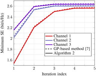
Figure 1: Convergence of Algorithm 2 and the GP-based algorithm for three random channel realizations. The relevant parameters are taken as $M=150,K=20,L=1,D=1$.

We can see that both methods reach almost the same objective for all three considered channel realizations. The marginal difference is due to a moderate value of the smoothness parameter $\tau$ in (21). The main advantage of our proposed method over the GP-based method is that each iteration of the proposed method is very memory efficient and computationally cheap, and hence, can be executed very fast. As a result, the total run-time of the proposed method is far less than that of the GP-based method as shown in Table I. In Table I, we report the actual run-time of both methods to solve the max-min problem. Here, we run our codes on a 64-bit Windows operating system with 16 GB RAM and Intel CORE i7, 3.7 GHz. Both iterative methods are terminated when the difference of the objective for the latest two iterations is less than $10^{-5}$.

TABLE I: Comparison of run-time (in seconds) between Algorithm 2 and the GP-based method. Here, $K=20$ and $D=1$.

APs	GP-based Method	Proposed Method
120	3.67	0.80
160	3.79	1.21
200	4.08	1.86
240	4.42	2.45

In the next experiment, we plot the cumulative distribution function (CDF) of the per-user SE (bit/s/Hz) for $300$ channel realizations shown in Fig. 2. We consider two large-scale scenarios: (i) $K=25,M=500$ and (ii) $K=50,M=1000$. Note that the ratio between the number of APs to the number of users is the same for two cases. It can be seen in Fig. 2 that as the number of the users increases, the per-use SE slightly decreases. We also observe that the per-user SE differs in the range of 0.1 bit/s/Hz which means that the fairness is indeed achieved among the users.

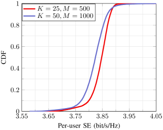
Figure 2: CDF of per-user achievable SE for two scenarios $K=25,M=500$ and $K=50,M=1000$. The number of antennas at each AP is $L=1$.

Finally, we investigate the effect of increasing the number of antennas per AP on the minimum achievable SE. Specifically, we plot the minimum achievable SE with respect to the number of antennas for both $M=250$ and $M=500$ APs. The number of users is fixed to $K=50$. As expected, the minimum achievable SE increases with the number of antennas per AP but the increase tends to be small when the number of antennas is sufficiently large. The reason is that for a large number of APs channel harderning and favorable propagation can be achieved by a few antennas per AP. Specifically, we can see that the SE for the case of $500$ APs and $5$ antennas per AP is larger than the SE for the case of 250 APs and 10 antennas per AP. Therefore, for large-scale cell-free massive MIMO having more APs with a few antennas each tends to be more beneficial than having fewer APs with more antennas each.

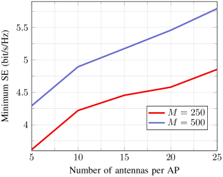
Figure 3: Maximized minimum achievable SE with respect to the number of antenna at each AP for $K=50,D=1.$

V Conclusion

In this paper, we have proposed a low-complexity method for maximizing the minimum achievable SE in the uplink of the cell free massive MIMO subject to per-user power constraint, assuming the MRC technique at APs. As in previous studies, we have divided the min-max problem into two subproblems: the receiver coefficient design and the power control problem. For the power control problem, the existing solutions rely on GP which requires high complexity. To overcome this issue, we have reformulated the power control problem into a convex form and then proposed an efficient numerical algorithm based on Nesterov’s smoothing technique and APG. Our proposed solution only requires the first order information of the objective and the projection, both of which are given in the closed-form. We have numerically shown that our proposed solution practically achieves the same objective as the GP-based method but in much lesser time. We have used the proposed method to study the performance of the large-scale systems up to 1000 APs for which the known methods are not suitable. We have also shown that a large-scale cell-free massive MIMO having more APs with a few antennas has better performance than a similar system having a fewer APs with more antennas per AP.

In this appendix, we show that the complexity of computing $\mathbf{u}_{k}$ is $\mathcal{O}(KM^{2})$. Without loss of generality, let us consider the inverse of $\mathbf{B}_{k}$ for user $1$. It is obvious that we can write $\mathbf{B}_{1}^{-1}$ as

$$\mathbf{B}_{1}^{-1} =\Bigl{(}\sum_{i=2}^{K}\boldsymbol{\nu}_{1i}\boldsymbol{\nu}_{1i}^{\mbox{\scriptsize H}}\eta_{i}+\tilde{\mathbf{D}}_{1}\Bigr{)}^{-1}$$

$$=\tilde{\mathbf{D}}_{1}^{-1}-\frac{\tilde{\mathbf{D}}_{1}^{-1}\boldsymbol{\nu}_{12}\boldsymbol{\nu}_{12}^{\mbox{\scriptsize H}}\tilde{\mathbf{D}}_{1}^{-1}}{1+\boldsymbol{\nu}_{12}^{\mbox{\scriptsize H}}\mathbf{D}_{k}^{-1}\boldsymbol{\nu}_{12}}$$ (26)

where $\tilde{\mathbf{D}}_{1}=\frac{1}{L}\sum_{i=1}^{K}\mathbf{D}_{1i}\eta_{i}+\frac{1}{L}\mathbf{R}_{1}+\sum_{i=3}^{K}\boldsymbol{\nu}_{1i}\boldsymbol{\nu}_{1i}^{\mbox{\scriptsize H}}\eta_{i}$. If we further express $\tilde{\mathbf{D}}_{1}$ in terms of the inverse of $\frac{1}{L}\sum_{i=1}^{K}\mathbf{D}_{1i}\eta_{i}+\frac{1}{L}\mathbf{R}_{1}+\sum_{i=4}^{K}\boldsymbol{\nu}_{1i}\boldsymbol{\nu}_{1i}^{\mbox{\scriptsize H}}\eta_{i}$ and keep on repeating this step, then finally we need to compute the inverse of the term $\frac{1}{L}\sum_{i=1}^{K}\mathbf{D}_{1i}\eta_{i}+\frac{1}{L}\mathbf{R}_{1}$ which is a diagonal matrix, and thus only requires $\mathcal{O}(M)$. The complexity of each step in the above process is $\mathcal{O}(M^{2})$, and thus the computation of $\mathbf{B}_{1}^{-1}$ is $\mathcal{O}\bigl{(}(K-1)M^{2}\bigr{)}$. Multiplying $\mathbf{B}_{1}^{-1}$ with $\boldsymbol{\nu}_{11}$ to obtain $\mathbf{u}_{1}$ takes additional $\mathcal{O}(M)$, and thus, the complexity of the computation of $\mathbf{u}_{1}$ stands at $\mathcal{O}\bigl{(}KM^{2}\bigr{)}$.

References

- [1] H. Q. Ngo, A. Ashikhmin, H. Yang, E. G. Larsson, and T. L. Marzetta, “Cell-free massive MIMO versus small cells,” IEEE Trans. Wireless Commun., vol. 16, no. 3, pp. 1834–1850, 2017.
- [2] H. Q. Ngo, H. Tataria, M. Matthaiou, S. Jin, and E. G. Larsson, “On the performance of cell-free massive MIMO in ricean fading,” in IEEE ACSSC 2018, 2018, pp. 980–984.
- [3] T. C. Mai, H. Q. Ngo, and T. Q. Duong, “Uplink spectral efficiency of cell-free massive MIMO with multi-antenna users,” in IEEE SigTelCom 2019, 2019, pp. 126–129.
- [4] W. A. C. W. Arachchi, K. B. S. Manosha, N. Rajatheva, and M. Latva-aho, “An alternating algorithm for uplink max-min SINR in cell-free massive MIMO with local-MMSE receiver,” arXiv: Information Theory, 2019.
- [5] M. Bashar, K. Cumanan, A. G. Burr, H. Q. Ngo, and H. V. Poor, “Mixed quality of service in cell-free massive MIMO,” IEEE Commun. Lett., vol. 22, no. 7, pp. 1494–1497, 2018.
- [6] M. Bashar, K. Cumanan, A. G. Burr, M. Debbah, and H. Q. Ngo, “Enhanced max-min SINR for uplink cell-free massive MIMO systems,” in IEEE ICC 2018, 2018, pp. 1–6.
- [7] M. Bashar, K. Cumanan, A. G. Burr, M. Debbah, and H. Q. Ngo, “On the uplink max-min SINR of cell-free massive MIMO systems,” IEEE Trans. Wireless Commun., vol. 18, no. 4, pp. 2021–2036, 2019.
- [8] M. Bashar, K. Cumanan, A. G. Burr, H. Q. Ngo, E. G. Larsson, and P. Xiao, “Energy efficiency of the cell-free massive MIMO uplink with optimal uniform quantization,” IEEE Trans. Green Commun. Netw., vol. 3, no. 4, pp. 971–987, 2019.
- [9] Y. Zhang, H. Cao, M. Zhou, and L. Yang, “Spectral efficiency maximization for uplink cell-free massive MIMO-NOMA networks,” in IEEE ICC 2019 Workshops, 2019, pp. 1–6.
- [10] Y. Nesterov, “Smooth minimization of non-smooth functions,” Math. Program., Ser. A, vol. 103, pp. 127–152, 2005.
- [11] E. Björnson, J. Hoydis, and L. Sanguinetti, Massive MIMO Networks: Spectral, Energy, and Hardware Efficiency. Now Foundations and Trends, 2017.
- [12] A. Beck and M. Teboulle, “A fast iterative shrinkage-thresholding algorithm for linear inverse problems,” SIAM Journal on Imaging Sciences, vol. 2, no. 1, pp. 183–202, 2009.
- [13] M. Farooq, H. Q. Ngo, and L. N. Tran, “Accelerated projected gradient method for the optimization of cell-free massive MIMO downlink,” in IEEE PIMRC 2020, 2020, pp. 1–6.
- [14] M. ApS, The MOSEK optimization toolbox for MATLAB manual. Version 7.1 (Revision 28)., 2015.
- [15] M. Grant and S. Boyd, “CVX: Matlab software for disciplined convex programming, version 2.1,” Mar. 2014.