Finite-amplitude method for collective inertia in spontaneous fission

Abstract

Background

Microscopic description of spontaneous fission is one of the most challenging subjects in nuclear physics. It is necessary to evaluate the collective potential and the collective inertia along a fission path for a description of quantum tunneling in spontaneous or low-energy fission. In past studies of the fission dynamics based on nuclear energy density functional (EDF) theory, the collective inertia has been evaluated with the cranking approximation, which neglects dynamical residual effects.

Purpose

The purpose is to provide a reliable and efficient method to include dynamical residual effects in the collective inertia for fission dynamics.

Methods

We use the local quasiparticle random-phase approximation (LQRPA) to evaluate the collective inertia along a fission path obtained by the constrained Hartree-Fock-Bogoliubov method with the Skyrme EDF. The finite-amplitude method (FAM) with a contour integration technique enables us to efficiently compute the collective inertia in a large model space.

Results

We evaluate the FAM-QRPA collective inertia along a symmetric fission path in ²⁴⁰Pu and ²⁵⁶Fm. The FAM-QRPA inertia is significantly larger than the one of the cranking approximation, and shows pronounced peaks around the ground state and the fission isomer. This is due to dynamical residual effects.

Conclusions

To describe the spontaneous or low-energy fission, we provide a reliable and efficient method to construct the collective inertia with dynamical residual effects that have been neglected in most of EDF-based works in the past. We show the importance of dynamical residual effects to the collective inertia. This work will be a starting point for a systematic study of fission dynamics in heavy and superheavy nuclei to microscopically describe the nuclear large-amplitude collective motions.

I Introduction

Nuclear fission [1, 2] plays an important role in various phenomena such as synthesis of superheavy elements [3, 4] and $r$-process nucleosynthesis in the universe [5, 6]. The fission governs the existence and decay property of superheavy nuclei. Various types of fission, such as neutron-induced fission, spontaneous fission, and $\beta$-delayed fission that involve neutron-rich heavy and superheavy nuclei, are important in expected environment in the $r$-process.

Theoretically, a microscopic description of large-amplitude collective motions, such as nuclear fission and fusion, is one of the challenging subjects in quantum many-body physics. Of particular interest is a quantum many-body tunneling for spontaneous or low-energy fission and subbarrier fusion of complex nuclei.

The most promising candidate for the microscopic approach is the selfconsistent nuclear energy density functional (EDF) theory [7, 8]. It is well established that the nuclear EDF gives a good description of ground-state properties of nuclei in the whole nuclear chart. The EDF approaches to the spontaneous fission have used a semiclassical description with the WKB approximation for quantum tunneling. These studies show how the result depends on the choice of relevant collective variables, the collective potential energy, and the collective inertia entering the action integral in the WKB approximation. The potential energy has been calculated by the Hartree-Fock-Bogoliubov method with constraints on the collective variables. On the other hand, the collective inertia used in the previous EDF-based works [9, 10, 11, 12, 13] is insufficient in the following respect: First of all, the previous works employ the so-called cranking approximation to the adiabatic time-dependent Hartree-Fock-Bogoliubov (ATDHFB) method [14] to evaluate the collective inertia. The cranking approximation neglects dynamical residual effects, especially, the time-odd terms of the EDF. This gives a big drawback, namely, the violation of the (local) Galilean symmetry, which leads to the incorrect total mass for the translational motion [15, 8]. The rotational moments of inertia of deformed nuclei are not properly given in the cranking approximation [16]. In addition, the collective inertia of the cranking approximation significantly deviates from the one including the dynamical residual effects [17]. Irrespective of such drawbacks, because of its simplicity, the cranking approximation has been widely used in evaluating collective inertia not only for fission dynamics but also for the collective Hamiltonian method [18, 19, 20, 21, 22]. It should be noted that the enhancement factors of $1.2$–$1.4$ are often adopted to correct the missing residual effect.

An alternative method to ATDHFB for describing large-amplitude collective motions has been developed, called the adiabatic selfconsistent collective coordinate (ASCC) method [23]. Based on the ASCC method, an efficient and feasible method to construct the collective Hamiltonian has been proposed [24]. In this method, the collective path (subspace) is determined by the constrained HFB (CHFB) calculation, while the collective inertia (the vibrational mass in the vibrational kinetic Hamiltonian) is determined by local normal modes built on CHFB states. Local normal modes are obtained by solving local quasiparticle random-phase approximation (LQRPA) equations. Dynamical residual effects with time-odd components are selfconsistently included in the collective inertia by the LQRPA. This method, called CHFB + LQRPA, has been applied to constructing five-dimensional quadrupole collective Hamiltonian for triaxial shapes with the pairing-plus-quadrupole (P+Q) Hamiltonian [24, 25, 26, 27], a hybrid model of the P+Q Hamiltonian and covariant EDF [28], and three-dimensional quadrupole collective Hamiltonian for axially symmetric shapes with the Skyrme EDF [29]. Those works have shown the importance of including dynamical residual effects with time-odd components on the description of large-amplitude collective motion.

Despite many evidences for the importance of dynamical residual effects, no practical application based on the ATDHFB method takes into account residual effects in the calculation of the collective inertia. The reason is that it requires huge numerical computations to apply directly the ATDHFB (or LQRPA) formulas to the collective inertia in realistic cases, due to the size of matrices treated with modern EDFs.

A method to efficiently solve the QRPA equations based on linear response theory has been developed for the EDF, called the finite-amplitude method (FAM) [30]. In the FAM, response functions to an external one-body field can be obtained only with one-body induced densities and fields with an iterative scheme. The FAM requires matrices with the size of approximately $N\times N$, while the QRPA equation requires those with the size $\approx N^{2}\times N^{2}$, where $N$ represents the number of single-particle basis. $N$ may exceeds $10^{3}$ when, for example, 20 major shells in the harmonic oscillator basis are used in solving deformed HFB equations. Thus, the computational cost of the FAM is significantly lower than that of QRPA. As an alternative way of solving the QRPA equations, the FAM has been employed in various applications [31, 32, 33, 34, 35, 36, 37, 38, 39, 40, 41, 42, 43, 44].

The standard FAM formalism has been extended to the one in terms of the momentum–coordinate (PQ) representation [45] to treat zero-energy modes of QRPA solutions known as spurious modes or Nambu–Goldstone (NG) modes [46, 47] associated with spontaneous symmetry breaking of the mean field. A general method to calculate the inertia of the NG modes was also given [45], which was applied to pairing rotation [48, 49] and to spatial rotation of axially deformed [50] and of triaxially deformed nuclei [51]. It is important to note that this formulation can treat imaginary solutions of the QRPA that may appear in the LQRPA at nonequilibrium HFB states obtained by the CHFB calculations.

The main aim of this paper is to propose a new method to efficiently evaluate the collective inertia used in the WKB approximation for spontaneous fission and in the vibrational kinetic terms in the collective Hamiltonian method. The method is based on the CHFB + LQRPA with the Skyrme EDF. We employ the PQ representation of the FAM to efficiently solve the LQRPA equations. We extend a contour integration approach of the FAM proposed in Ref. [36] to compute the collective inertia associated with the most collective local normal mode in the LQRPA.

This paper is organized as follows. Section II briefly summarizes the formulations of the collective inertia in ATDHFB with the cranking approximation and in the LQRPA. In Sec. III, we explain the formulation of the CHFB + LQRPA with the FAM to calculate the collective inertia. In Sec. IV, we present the results of the collective inertia along mass-symmetric fission path in ²⁴⁰Pu and ²⁵⁶Fm and comparison between our results and those with the cranking approximation. Conclusions are given in Sec. V.

II Collective inertia with EDF

II.1 ATDHFB

We give a brief explanation for the collective inertia in ATDHFB. For details, we refer to Refs. [14, 17, 9, 13].

In ATDHFB, the collective motion of the system is assumed to be described by a set of a few collective coordinates $s_{i}$ and its conjugate momenta. The collective coordinates are defined as $s_{i}=\langle\phi(s)|\hat{s}_{i}|\phi(s)\rangle$, where $\hat{s}_{i}$ are generators driving the collective motion. In practice, the collective subspace $\ket{\phi(s)}$ is determined by the CHFB calculation with the constraint on $s_{i}$. Most applications take $\hat{s}_{i}$ as one-body operators of multipole moments. The ATDHFB relies on the assumption that the collective velocities of the system denoted by the time derivative of the collective coordinates, $\dot{s}_{i}$, are slow enough to make adiabatic assumption valid. The expression of the collective inertia tensor in ATDHFB is given by

$$\mathcal{M}_{ij}=\frac{i}{2\dot{s}_{i}\dot{s}_{j}}\text{Tr}(F^{i*}Z^{j}-F^{i}Z^{j*}).$$ (1)

The matrix $Z$ involves time-odd fields associated with time-odd density matrices. A standard method to determine the matrix $Z$ requires solution of the QRPA equation. The matrix $F$ is evaluated by

$$\frac{F^{i}}{\dot{s}_{i}}=U^{\dagger}\frac{\partial\rho}{\partial s_{i}}V^{*}+U^{\dagger}\frac{\partial\kappa}{\partial s_{i}}U^{*}-V^{\dagger}\frac{\partial\rho^{*}}{\partial s_{i}}U^{*}-V^{\dagger}\frac{\partial\kappa^{*}}{\partial s_{i}}V^{*},$$ (2)

where $U$ and $V$ are the Bogoliubov transformation matrices and $\rho$ and $\kappa$ are the density matrix and pairing tensor, respectively. This expression includes derivatives of density matrices with respect to the collective coordinates.

II.1.1 Cranking approximation

The cranking approximation neglects the time-odd fields in the collective inertia (1). In this case, the matrix $Z^{i}$ can be simply written in terms of $F^{i}$ and the quasiparticle energies. The collective inertia tensor of the cranking approximation then reads in the quasiparticle basis

$$\mathcal{M}_{ij}^{\text{C}}=\frac{1}{2\dot{s}_{i}\dot{s}_{j}}\sum_{\mu\nu}\frac{(F_{\mu\nu}^{i*}F_{\mu\nu}^{j}+F_{\mu\nu}^{i}F_{\mu\nu}^{j*})}{E_{\mu}+E_{\nu}},$$ (3)

where $E_{\mu}$ and $E_{\nu}$ are one-quasiparticle energies defined with respect to the constrained Hamiltonian of the form of Eq. (7) and the CHFB state $\ket{\phi(s)}$ of Eq. (6).

II.1.2 Perturbative cranking approximation to ATDHFB

Further approximation leads to the so-called perturbative cranking approximation, where the derivatives of the densities with respect to the collective coordinates in Eq. (2) are not explicitly evaluated, but are obtained in a perturbative manner. The expression of the collective inertia in the perturbative cranking approximation is given as

$$\mathcal{M}^{\text{PC}}=\frac{1}{2}[M^{(1)}]^{-1}M^{(3)}[M^{(1)}]^{-1},$$ (4)

where the $n$-th energy-weighted moment $M^{(n)}$ is given as

$$M_{ij}^{(n)}=\sum_{\mu<\nu}\frac{\langle\phi(s)|\hat{s}_{i}|\mu\nu\rangle\langle\mu\nu|\hat{s}_{j}^{\dagger}|\phi(s)\rangle}{(E_{\mu}+E_{\nu})^{n}},$$ (5)

where $|\mu\nu\rangle$ are two-quasiparticle states based on the CHFB state $\ket{\phi(s)}$.

II.2 CHFB + Local QRPA

Another method to evaluate the collective inertia is the CHFB + LQRPA [24] derived from the ASCC method [23]. Suppose that a set of $N$ collective coordinates $q_{i}$ ($i=1,\cdots,N$) selfconsistently determined with the ASCC method can be mapped to a set of $N$ collective variables $s_{m}$ ($m=1,\cdots,N$) through a one-to-one correspondence between them. In addition, we assume that the ASCC collective subspace can be approximated by the one obtained with the CHFB calculation with a given set of constraining operators $\hat{s}_{m}$. The CHFB equation is given by

$$\delta\langle\phi(s)|\hat{H}_{M}|\phi(s)\rangle=0,$$ (6)

with the constrained Hamiltonian

$$\hat{H}_{M}=\hat{H}-\sum_{\tau=n,p}\lambda_{\tau}\hat{N}_{\tau}-\sum_{m}\lambda_{m}\hat{s}_{m},$$ (7)

where $\lambda_{n,p}$ denote the Fermi energies for neutrons and protons to constrain the average neutron and proton numbers $\bra{\phi(s)}\hat{N}_{\tau}\ket{\phi(s)}$ ($\tau=n,p$) and $\lambda_{m}$ are the Lagrange multipliers of constraining $\langle\phi(s)|\hat{s}_{m}|\phi(s)\rangle=s_{m}$. The energy minimization, Eq. (6), leads to the CHFB state $|\phi(s)\rangle$ and collective potential $V(s)=\langle\phi(s)|\hat{H}|\phi(s)\rangle$. At each CHFB state $|\phi(s)\rangle$, the LQRPA equations,

$$\delta\langle\phi(s)|[\hat{H}_{M},\hat{Q}_{i}(s)]-\frac{1}{i}\hat{P}_{i}(s)|\phi(s)\rangle =0,$$ (8)

$$\delta\langle\phi(s)|[\hat{H}_{M},\frac{1}{i}\hat{P}_{i}(s)]-\Omega_{i}^{2}(s)\hat{Q}_{i}(s)|\phi(s)\rangle =0,$$ (9)

are solved to determine $\hat{Q}_{i}(s)$ and $\hat{P}_{i}(s)$ that are local generators of collective momenta and coordinates, respectively, defined at $s$. They should satisfy the weak canonicity condition, Eq. (19). Here, the inertial and the curvature tensors are diagonalized to define the local normal mode. Furthermore, in order to fix the arbitrary scale of the collective coordinate $q_{i}$, the inertia with respect to $q_{i}$ is set to be unity, ${\cal M}_{ij}=\delta_{ij}$. $\Omega^{2}_{i}(s)$ denotes the squared eigenfrequency of the local normal mode. Note that the eigenfrequency of the LQRPA equations can be imaginary ($\Omega^{2}_{i}(s)<0$) at nonequilibrium CHFB states. A criterion for selecting relevant collective LQRPA modes from many LQRPA solutions is given in Ref. [24].

Once relevant LQRPA collective modes are selected, the collective inertia tensor is given as follows. First, the collective kinetic energy is expressed as

$$T=\frac{1}{2}\sum_{i}\dot{q}_{i}^{2}=\frac{1}{2}\sum_{mn}{\cal M}_{mn}(s)\dot{s}_{m}\dot{s}_{n},$$ (10)

where collective inertia tensor $\mathcal{M}_{mn}(s)$ is defined by the transformation of the collective coordinates $q_{i}$ to the collective variables $s$,

$$\mathcal{M}_{mn}(s)\equiv\sum_{i,j}\frac{\partial q_{i}}{\partial s_{m}}{\cal M}_{ij}\frac{\partial q_{j}}{\partial s_{n}}=\sum_{i}\frac{\partial q_{i}}{\partial s_{m}}\frac{\partial q_{i}}{\partial s_{n}}.$$ (11)

Second, the partial derivatives in Eq. (11) are evaluated using the local generator $\hat{P}_{i}(s)$ of the LQRPA solution as

$$\frac{\partial s_{m}}{\partial q_{i}} =\frac{\partial}{\partial q_{i}}\langle\phi(s)|\hat{s}_{m}|\phi(s)\rangle$$

$$=\langle\phi(s)|[\hat{s}_{m},\frac{1}{i}\hat{P}_{i}(s)]|\phi(s)\rangle,$$ (12)

which is calculable without numerical derivatives.

III Finite-amplitude method for collective inertia

In this work, we use the LQRPA method to evaluate the collective inertia along a fission path. Since it is computationally hard to solve the LQRPA equations for deformed nuclear shapes with the Skyrme EDF, we employ the FAM to efficiently solve the LQRPA equations. In this section, we explain our method to obtain the expression of the collective inertia based on the FAM and LQRPA.

III.1 Finite-amplitude method

Here, the FAM is recapitulated. The details of its derivation can be found in Refs. [30, 32]. The FAM equations can be expressed in the quasiparticle basis as

$$(E_{\mu}+E_{\nu}-\omega)X_{\mu\nu}(\omega)+\delta H^{20}_{\mu\nu}(\omega) =-F^{20}_{\mu\nu}\;,$$ (13a)

$$(E_{\mu}+E_{\nu}+\omega)Y_{\mu\nu}(\omega)+\delta H^{02}_{\mu\nu}(\omega) =-F^{02}_{\mu\nu}\;,$$ (13b)

where $X_{\mu\nu}(\omega)$ and $Y_{\mu\nu}(\omega)$ are the FAM amplitudes at a given frequency $\omega$, and $\delta H^{20(02)}_{\mu\nu}$ and $F^{20(02)}_{\mu\nu}$ are two-quasiparticle components of one-body induced field $\delta\hat{H}$ and an external field $\hat{F}$, respectively. The FAM equations (13) are iteratively solved at each $\omega$ until converged $X$ and $Y$ amplitudes are obtained. Complex frequency $\omega$ is usually used with the imaginary part corresponding to a smearing width. Only one-body quantities (induced densities and induced fields) are necessary to solve the FAM equations.

The FAM strength function is given from converged $X$ and $Y$ amplitudes as

$$S(\hat{F},\omega)=\sum_{\mu<\nu}\left[F_{\mu\nu}^{20*}X_{\mu\nu}(\omega)+F_{\mu\nu}^{02*}Y_{\mu\nu}(\omega)\right].$$ (14)

Taking the frequency $\omega$ real and positive, the transition strength distribution is given as

$$\frac{dB(\hat{F},\omega)}{d\omega}\equiv\sum_{i(\Omega_{i}>0)}\left|\bra{i}\hat{F}\ket{0}\right|^{2}\delta(\omega-\Omega_{i})=-\frac{1}{\pi}\text{Im}S(\hat{F},\omega),$$ (15)

where $\ket{0}$ is the QRPA vacuum and $\ket{i}\equiv\hat{O}_{i}^{\dagger}\ket{0}$ is a state of the QRPA normal mode of excitation with the eigenfrequency $\Omega_{i}$.

The relation between the FAM strength function (14) and the QRPA transition strength $|\langle i|\hat{F}|0\rangle|^{2}$ between the ground state and a QRPA eigenstate $\ket{i}$ is given as [36]

$$S(\hat{F},\omega)=-\sum_{i(\Omega_{i}>0)}\left(\frac{|\langle i|\hat{F}|0\rangle|^{2}}{\Omega_{i}-\omega}+\frac{|\langle 0|\hat{F}|i\rangle|^{2}}{\Omega_{i}+\omega}\right).$$ (16)

III.2 FAM in the PQ representation

In Ref. [45], the FAM in the PQ representation of the QRPA was formulated to investigate the NG modes and the Thouless–Valatin inertia of the NG modes. In this subsection, we summarize the formulation of the FAM in the PQ representation.

In the PQ representation of the QRPA, the coordinate and the conjugate momentum operators, $\hat{Q}_{i}$ and $\hat{P}_{i}$, which are both Hermitian, are constructed from the QRPA phonon operators $(\hat{O}_{i},\hat{O}^{\dagger}_{i})$ as

$$\hat{Q}_{i} =\sqrt{\frac{1}{2M_{i}\Omega_{i}}}(\hat{O}_{i}+\hat{O}^{\dagger}_{i}),$$ (17)

$$\hat{P}_{i} =\frac{1}{i}\sqrt{\frac{M_{i}\Omega_{i}}{2}}(\hat{O}_{i}-\hat{O}^{\dagger}_{i}),$$ (18)

where $M_{i}$ is the inertia parameter. The operators $\hat{Q}_{i}$ and $\hat{P}_{i}$ fulfill the following commutation relations,

$$\bra{0}[\hat{Q}_{i},\hat{P}_{j}]\ket{0}=i\delta_{ij},\;\bra{0}[\hat{Q}_{i},\hat{Q}_{j}]\ket{0}=\bra{0}[\hat{P}_{i},\hat{P}_{j}]\ket{0}=0,$$ (19)

which guarantee the orthogonality among different normal modes, however, their scale is still arbitrary as $(\alpha\hat{Q}_{i},\alpha^{-1}\hat{P}_{i})$. In the present study, this scale is fixed by imposing the additional condition, $M_{i}=1$.

Using two-quasiparticle components $P_{\mu\nu}^{i}$ and $Q_{\mu\nu}^{i}$ of the operators $\hat{P}_{i}$ and $\hat{Q}_{i}$, the FAM $X$ and $Y$ amplitudes are given as

$$X_{\mu\nu}(\omega)= \sum_{i}\frac{1}{\omega^{2}-\Omega^{2}_{i}}\Bigl{[}(-i\omega P_{\mu\nu}^{i}+\Omega_{i}^{2}Q_{\mu\nu}^{i})q_{i}(\hat{F})$$

$$\qquad+(P_{\mu\nu}^{i}+i\omega Q_{\mu\nu}^{i})p_{i}(\hat{F})\Bigr{]},$$ (20a)

$$Y_{\mu\nu}(\omega)= \sum_{i}\frac{1}{\omega^{2}-\Omega^{2}_{i}}\Bigl{[}(i\omega P_{\mu\nu}^{i*}-\Omega_{i}^{2}Q_{\mu\nu}^{i*})q_{i}(\hat{F})$$

$$\qquad+(-P_{\mu\nu}^{i*}-i\omega Q_{\mu\nu}^{i*})p_{i}(\hat{F})\Bigr{]},$$ (20b)

where $p_{i}(\hat{F})$ and $q_{i}(\hat{F})$ are defined as

$$p_{i}(\hat{F}) \equiv\bra{0}[\hat{P}_{i},\hat{F}]\ket{0}=\sum_{\mu<\nu}\left(P_{\mu\nu}^{i*}F_{\mu\nu}^{20}-P_{\mu\nu}^{i}F_{\mu\nu}^{02}\right),$$ (21)

$$q_{i}(\hat{F}) \equiv\bra{0}[\hat{Q}_{i},\hat{F}]\ket{0}=\sum_{\mu<\nu}\left(Q_{\mu\nu}^{i*}F_{\mu\nu}^{20}-Q_{\mu\nu}^{i}F_{\mu\nu}^{02}\right).$$ (22)

The FAM strength function (14) is then rewritten as

$$S(\hat{F},\omega) =\sum_{\mu<\nu}\left[F_{\mu\nu}^{20*}X_{\mu\nu}(\omega)+F_{\mu\nu}^{02*}Y_{\mu\nu}(\omega)\right]$$

$$=\sum_{i}\frac{1}{\omega^{2}-\Omega^{2}_{i}}\left[|p_{i}(\hat{F})|^{2}+\Omega_{i}^{2}|q_{i}(\hat{F})|^{2}+\omega\;r_{i}(\hat{F})\right],$$ (23)

with a real quantity

$$r_{i}(\hat{F})\equiv i\left[q_{i}^{*}(\hat{F})p_{i}(\hat{F})-q_{i}(\hat{F})p_{i}^{*}(\hat{F})\right].$$ (24)

The FAM $X(\omega)$ and $Y(\omega)$ amplitudes (20) and the FAM strength function (23) are defined in the whole complex plane $\omega$ except for $\omega=\pm\Omega_{i}$. They are well defined even with the presence of the NG modes ($\Omega_{i}^{2}=0$) and the imaginary solutions ($\Omega_{i}^{2}<0$) which can appear in the LQRPA at nonequilibrium CHFB states.

III.3 Collective inertia with FAM plus contour integration technique

For simplicity, in this paper, we assume only one collective coordinate $q$, and then adopt the isoscalar quadrupole moment $\hat{s}=\hat{Q}_{20}=\sqrt{16\pi/5}\sum_{i=1}^{A}r_{i}^{2}Y_{20}(\hat{\boldsymbol{r}}_{i})$ as the constraint. For the LQRPA calculation, we adopt the same operator for the external field $\hat{F}=\hat{Q}_{20}$. Then, by transforming the scale of the coordinate from $q$ to $s=\bra{\phi(s)}\hat{Q}_{20}\ket{\phi(s)}$, the expression of the collective inertia (11) becomes

$${\cal M}\equiv\frac{dq}{ds}\frac{dq}{ds},$$ (25)

with $dq/ds=(ds/dq)^{-1}$ and

$$\frac{ds}{dq} =\langle\phi(s)|[\hat{Q}_{20},\frac{1}{i}\hat{P}_{i}]|\phi(s)\rangle$$

$$=ip_{i}(\hat{Q}_{20}).$$ (26)

We will see below that $p_{i}(\hat{Q}_{20})$ is pure imaginary, leading to real $ds/dq$. We select the normal mode $i$ which has the largest value of $|p_{i}(\hat{Q}_{20})|^{2}$ among the low-lying eigenmodes.

The remaining task is the calculation of $p_{i}(\hat{F})=p_{i}(\hat{Q}_{20})$ in the FAM. From Eqs. (17) and (18), $P^{i}$ and $Q^{i}$ are given in terms of the forward and backward amplitudes of the QRPA normal modes, $X^{i}$ and $Y^{i}$, as

$$P_{\mu\nu}^{i} =i\sqrt{\frac{\Omega_{i}}{2}}(X_{\mu\nu}^{i}+Y_{\mu\nu}^{i}),$$ (27)

$$Q_{\mu\nu}^{i} =\sqrt{\frac{1}{2\Omega_{i}}}(X_{\mu\nu}^{i}-Y_{\mu\nu}^{i}).$$ (28)

Note that we set $M_{i}=1$. When the QRPA matrices are real, we may choose $X^{i}_{\mu\nu}$ and $Y^{i}_{\mu\nu}$ real. This leads to real $Q^{i}_{\mu\nu}$ and pure imaginary $P^{i}_{\mu\nu}$. In the present case, the external-field operator $\hat{F}=\hat{Q}_{20}$ is Hermitian and their two-quasiparticle components are real, namely, $F^{02}=F^{20*}=F^{20}$. Thus, $q_{i}(\hat{F})=0$ and $p_{i}(\hat{F})=-p_{i}^{*}(\hat{F})$ (pure imaginary) hold according to Eq. (22). Then, the FAM strength function (23) becomes

$$S(\hat{F},\omega)=\sum_{i}\frac{1}{\omega^{2}-\Omega^{2}_{i}}|p_{i}(\hat{F})|^{2}.$$ (29)

Since the right-hand side of Eq. (29) has first-order poles at $\omega=\pm\Omega_{i}$, we obtain the following expression using Cauchy’s integral formula,

$$\frac{1}{2\pi i}\oint_{C_{i}}\omega S(\hat{F},\omega)d\omega=\frac{1}{2}|p_{i}(\hat{F})|^{2},$$ (30)

where the contour circle $C_{i}$ in the complex energy plane is chosen to encircle only the pole $\omega=\Omega_{i}$. The strength functions, $S(\hat{F},\omega)$, at different values of $\omega$ are obtained as Eq. (14) with iterative solution of Eq. (13).

The eigenfrequency $\Omega_{i}$ can be also obtained by combining Eq. (30) with the following contour integration,

$$\frac{1}{2\pi i}\oint_{C_{i}}S(\hat{F},\omega)d\omega=\frac{1}{2\Omega_{i}}|p_{i}(\hat{F})|^{2}.$$ (31)

The expressions (30) and (31) can be used for both real and pure imaginary eigenfrequencies.

III.4 Numerical procedure

To prepare the CHFB states along the fission path, we solve the CHFB equations with the two-basis method [52, 53], where during iteration the HFB Hamiltonian is diagonalized in a single-particle basis that converges to the eigenstates of the mean-field Hamiltonian, called the Hartree-Fock (HF) basis, and the local densities are constructed in the canonical basis that diagonalizes the density matrix. The single-particle wave functions and fields are represented in a three-dimensional (3D) Cartesian mesh. Nuclear shapes are restricted to have three plane reflection symmetries about the $x=0$, $y=0$, and $z=0$ planes. This reduces the model space to 1/8 of the full box and can be realized by choosing the single-particle wave functions as eigenstates of parity, $z$ signature, and $y$ time simplex [54, 55, 56, 57]. This symmetry restriction prevents us from treating asymmetric fission in the present study. We use a numerical box of 13.2 fm for $x$ and $y$ directions and 19.6 fm for $z$ direction in $x>0$, $y>0$, and $z>0$ in order to express prolately deformed fissioning shapes, discretized with the mesh size of $0.8$ fm for all the directions. The number of mesh points then becomes $16\times 16\times 24=6144$. The single-particle basis consists of 2460 neutron and 1840 proton HF-basis states to achieve the maximum quasiparticle energy of $E_{\text{QP}}^{\text{max}}\approx 60$ MeV for both neutrons and protons in ²⁴⁰Pu and ²⁵⁶Fm. Constrained quantities are the isoscalar quadrupole moment $Q_{20}=\langle\hat{Q}_{20}\rangle$ with $\langle\hat{Q}_{22}\rangle=0$, keeping axially symmetric shapes. The symmetry restriction automatically constrains the position of the center of mass, and $\langle xy\rangle=\langle yz\rangle=\langle zx\rangle=0$. The other even multipole moments are not constrained, and their values are optimized to minimize the total energy, while the expectation values of all odd multipole moments are kept to be zero due to the plane reflection symmetries of nuclear shapes. We used the SkM^∗ EDF [58] and the contact volume pairing with a pairing window of 20 MeV above and below the Fermi energy in the HF basis described in Refs. [54, 56] to avoid divergence in the pairing energy. The pairing strengths are adjusted separately for neutrons and protons in order to reproduce the empirical pairing gaps in ²⁴⁰Pu or in ²⁵⁶Fm.

We have extended our 3D FAM-QRPA code developed in Ref. [44] to perform FAM calculations at CHFB states and the FAM-QRPA with the contour integration. We include in the FAM the full quasiparticle basis included in the CHFB calculations to satisfy full selfconsistency between the CHFB and LQRPA calculations. We employ the modified Broyden method [59] for iteratively solving the FAM equations.

To obtain the quantity $|p_{i}(\hat{F})|^{2}$ by the contour integration (30), it is necessary to know in advance an approximate position of each QRPA pole $\omega=\Omega_{i}$ in the complex energy plane for determining an appropriate contour $C_{i}$. The QRPA poles are expected to appear as sharp peaks in the FAM strength distribution. Therefore, we first calculate the FAM strength distribution (15) in the low-lying states with $\omega^{2}<16$ MeV². For each pole, we calculate $|p_{i}(\hat{F})|^{2}$ and adopt the most collective mode with the largest value of $|p_{i}(\hat{F})|^{2}$. A detail of our procedure of selecting the most collective mode in the FAM is given in Appendix. For the integration contour, we use a circle centered at the estimated peak frequency. The radius is 0.05 MeV for real solutions, and 0.1 MeV for an imaginary solution. If there are other poles close to the present pole, we use a circle with even smaller radius. The number of discretization points along the circle is 12 for real and 8 for imaginary solutions.

We perform numerical calculations of the FAM with a hybrid parallel scheme; The MPI parallelization is adopted for calculation of $S(\hat{F},\omega)$ at different $\omega$ points. The FAM iterative solution of Eq. (13) at each $\omega$ is performed using the OpenMP parallel calculation. It takes about 160 core hours on Oakforest-PACS for the FAM contour integration for a real solution at one deformation point with the present model space.

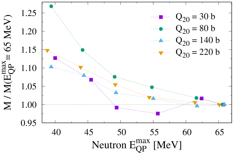
Figure 1: Collective inertia as a function of $E_{\text{QP}}^{\text{max}}$ for neutrons divided by that with neutron $E_{\text{QP}}^{\text{max}}\approx 65$ MeV for four different deformation points in ²⁴⁰Pu. Included neutron HF-basis states are 1200, 1440, 1632, 1998, 2460, and 2700 for $E_{\text{QP}}^{\text{max}}\approx 40$, 45, 50, 55, 60, and 65 MeV, respectively.

Before we proceed, we would like to discuss the convergence property of the collective inertia with respect to the size of the model space included in the ground state. To check the convergence property, we calculated the collective inertia with different numbers of HF-basis states corresponding to different $E_{\text{QP}}^{\text{max}}$ values in the ground state. Figure 1 shows the collective inertia as a function of neutron $E_{\text{QP}}^{\text{max}}$ (nearly equal to proton $E_{\text{QP}}^{\text{max}}$) divided by that calculated with neutron $E_{\text{QP}}^{\text{max}}\approx 65$ MeV as a reference value for four various deformation points in ²⁴⁰Pu. We find that the model space with neutron $E_{\text{QP}}^{\text{max}}\geq 55$ MeV gives a good convergence within about less than 5% to the value with $E_{\text{QP}}^{\text{max}}\approx 65$ MeV for the four various deformation points. Therefore, as mentioned above, we include 2460 neutron and 1840 proton HF-basis states corresponding to $E_{\text{QP}}^{\text{max}}\approx 60$ MeV in our calculations. Note again that we do not introduce in the FAM calculations the additional two-quasiparticle energy cutoff, which has been usually employed to reduce the dimension of the QRPA matrix.

IV Results

Mass distributions of fission fragments measured in low-energy fission show a sudden change from asymmetric to symmetric mass distributions when the neutron number changes. A well known example is Fm isotopes, where ²⁵⁶Fm shows an asymmetric mass distribution, while ${}^{258}\text{Fm}$ shows that the main component of fission fragments is a symmetric one [60, 61]. Even more complicated multi-mode or multi-channel fission has been observed and analyzed in the total-kinetic-energy distributions of fission fragments in actinides [62, 63]. What determines the mass distribution? It is still an open question, and the fragment mass distribution is important for the fission recycling of the $r$-process as well. Since, so far, most of studies are focused on the potential landscape, we aim at investigating effect of the collective inertia. In this section, we take ²⁴⁰Pu and ²⁵⁶Fm as examples to show importance of dynamical residual effects on the inertia. Although, in this paper, the calculation is performed only along the symmetric fission path, we will show that the residual effect on the inertia may hinder the symmetric fission probability.

IV.1 Collective inertia along a symmetric fission path in ²⁴⁰Pu

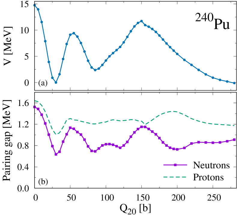
Figure 2: (a) Potential energy (b) pairing gaps for neutrons (solid line) and protons (dashed line) as a function of quadrupole moment $Q_{20}$ in units of barn in ²⁴⁰Pu.

Figure 2(a) shows the collective potential energy as a function of expectation value of quadrupole moment $Q_{20}$ in units of barn (b) along a symmetric fission path in ${}^{240}\text{Pu}$ obtained from the CHFB calculation. The ground state of ²⁴⁰Pu is found at $Q_{20}\approx 30$ b. The first fission barrier, the fission isomer (local minimum), and the second fission barrier are obtained at $Q_{20}\approx 55$ b, $Q_{20}\approx 85$ b, and $Q_{20}\approx 150$ b, respectively. We would like to note that the heights of the first and second fission barriers would become lower if we could include triaxial deformation for the first fission barrier and octupole deformation for the second fission barrier [64, 65]. Neutron and proton pairing gaps are shown along the fission path in Fig. 2(b). The neutron pairing gap becomes larger at the regions near the fission barriers and smaller near the ground state and fission isomer. The proton pairing gap shows a moderate behavior because of the difference between neutron and proton single-particle structures. It is known that transition strengths of low-lying modes are affected by the strength of pairing correlations.

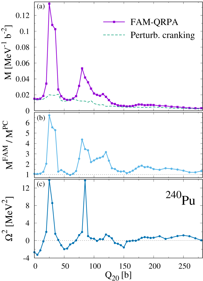
Figure 3: (a) Collective inertia of the FAM-QRPA calculation shown by the filled-square solid line, and of the perturbative cranking approximation by the dashed line, (b) ratio of the FAM-QRPA inertia to the perturbative cranking inertia, (c) squared QRPA eigenfrequency as a function of $Q_{20}$ in ²⁴⁰Pu.

Figure 3(a) shows the collective inertia obtained with the present FAM-QRPA calculation by the filled-square solid line. This shows two prominent peaks at $Q_{20}\approx 25$ b and $Q_{20}\approx 80$ b and a sudden change near these peaks. These states closely correspond to the ground state and the fission isomer observed in Fig. 2(a) and to the states where pairing becomes weak in Fig. 2(b). For comparison, we add in Fig. 3(a) the collective inertia obtained by the perturbative cranking approximation. It is clearly shown that the FAM-QRPA inertia is larger than the perturbative cranking inertia. We emphasize this point in Fig. 3(b), showing that the ratio of the FAM-QRPA inertia to the perturbative cranking inertia always exceeds unity, except at $Q_{20}=60$ b. This indicates that the action integral in the WKB approximation will be significantly affected by the increase of the collective inertia near the fission barriers. The behaviors of the two inertias are different; the FAM-QRPA inertia shows a strong variation, while the perturbative cranking inertia varies smoothly as $Q_{20}$ increases.

We estimate the action integral in the WKB approximation using the obtained collective inertia and potential along the symmetric fission path. The action integral reads

$$S=\int_{Q_{\text{in}}}^{Q_{\text{out}}}dQ_{20}\sqrt{2\mathcal{M}(Q_{20})[V(Q_{20})-E_{0}]},$$ (32)

where $Q_{\text{in}}$ and $Q_{\text{out}}$ are the classical inner and outer turning points, and $E_{0}$ is the HFB ground state energy. We obtain the action integrals $S_{\text{FAM}}=82.0$ for the FAM-QRPA inertia and $S_{\text{PC}}=62.0$ for the perturbative cranking inertia from $Q_{\text{in}}=30$ b (the ground state) to $Q_{\text{out}}=270$ b. This difference leads to many orders of magnitude difference in the fission half-life.

Figure 3(c) shows the eigenfrequency squared $\Omega^{2}$ of the LQRPA solution selected as the most collective mode at each deformation. This represents the curvature of the collective potential, which can indeed become negative at the fission barriers. Larger values of $\Omega^{2}$ are found at the states with larger values of the collective inertia. As $\Omega^{2}$ becomes larger, the ratio of the FAM-QRPA inertia to the perturbative cranking inertia becomes larger. When $\Omega^{2}$ are negative, the ratio is close to unity.

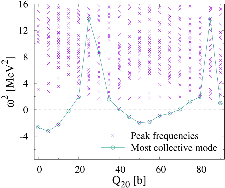
Figure 4: Squared peak frequencies identified from the FAM strength distribution shown by the crosses as a function of $Q_{20}$ in ²⁴⁰Pu. Eigenfrequency squared of the most collective mode is shown by the open-circle solid line.

In Fig. 4, we plot the squared peak frequencies identified from the FAM strength distribution in $\omega^{2}<16\,\text{MeV}^{2}$ as a function of $Q_{20}$ up to the fission isomer ($Q_{20}\leq 90$ b). Note that, because of a finite smearing width ($=0.01$ MeV) used in the FAM calculation, the identified peak frequencies may slightly differ from the QRPA eigenfrequencies and may not correspond to all the eigenfrequencies. In the figure, the eigenfrequency squared of the most collective mode that is used in the FAM-QRPA collective inertia is shown by the open-circle solid line. At most regions in $Q_{20}$, we find that the most collective mode corresponds to the lowest-frequency mode and is well separated from other peaks. On the other hand, around the ground state ($Q_{20}\approx 30$ b) and the fission isomer ($Q_{20}\approx 85$ b), where pairing becomes weak, we find that the most collective mode appears at frequencies close to other peaks, or at higher frequencies. The increase of the FAM-QRPA inertia near the ground and the fission isomer states is due to decrease of the quadrupole collectivity which leads to decrease in $|p_{i}(\hat{Q}_{20})|^{2}$. In fact, near the ground state, we find that the character of the lowest frequency mode changes from the quadrupole vibration to the pair vibration.

It is known that QRPA eigenmodes that possess pair-vibrational character tend to appear in low-frequency regions when pairing becomes weak. We analyze the character of the lowest-frequency mode at $\omega\sim 1.5$ MeV at $Q_{20}=25$, 30, and 35 b by using the FAM calculation with the pair-vibrational field as an external field. The lowest-frequency modes at $Q_{20}=25$, 30, and 35 b have a strong neutron pair-vibrational character and approximately satisfy the relation $\Omega\approx 2\Delta_{n}$, where $\Delta_{n}$ denotes the neutron pairing gap. The lowest-frequency modes at $Q_{20}=25$ and 30 b are not the most collective in the quadrupole $Q_{20}$ nature. We also confirm this by calculating the collective inertia for those lowest modes. For the lowest mode, the collective inertia would be $\mathcal{M}=0.190\,\text{MeV}^{-1}\text{b}^{-2}$ at $Q_{20}=25$ b and $\mathcal{M}=1.02\,\text{MeV}^{-1}\text{b}^{-2}$ at $Q_{20}=30$ b. These values are significantly larger than the values shown in Fig. 3(a), indicating the character change of the lowest mode from the quadrupole vibration to the neutron pair vibration.

IV.2 Comparison between the FAM-QRPA and nonperturbative cranking inertias in ²⁵⁶Fm

The aim of taking the ²⁵⁶Fm case is to compare the FAM-QRPA collective inertia with that of the nonperturbative cranking approximation by Baran et al. in Ref. [9]. In ²⁵⁶Fm, it is known that reflection-symmetric and reflection-asymmetric fission paths bifurcate at $Q_{20}\approx 130$ b [66, 67, 68]. In Ref. [9], the collective inertia was calculated along a reflection-symmetric fission path in $Q_{20}<130$ b and along a reflection-asymmetric fission path in $Q_{20}>130$ b. As we do not include reflection-asymmetric fission paths, we compare the FAM-QRPA collective inertia with that in Ref. [9] along the reflection-symmetric fission path in $Q_{20}\leq 130$ b.

Figure 5: Same as Fig. 2, but for ²⁵⁶Fm.

First, we show in Fig. 5 the potential and pairing gaps along an axial and reflection-symmetric fission path as a function of $Q_{20}$. The structure of a fission isomer at $Q_{20}\approx 110$ b almost vanishes due to low second fission barrier height of about 0.4 MeV. The proton pairing vanishes in $Q_{20}\geq 130$ b. These properties are consistent with previous EDF studies [66, 67, 68, 9].

Figure 6: (a) Comparison between the FAM-QRPA inertia (the filled-square solid line), the nonperturbative cranking inertia taken from Baran et al. [9] (the filled-triangle dot-dashed line), and the perturbative cranking inertia (dashed line), and (b) squared QRPA eigenfrequency as a function of $Q_{20}$ along a symmetric fission path in ²⁵⁶Fm.

Figure 6(a) shows the FAM-QRPA collective inertia as a function of $Q_{20}$. Two peaks in the FAM-QRPA inertia are clearly seen at the ground state ($Q_{20}\approx 30$ b) and fission isomer ($Q_{20}\approx 105$ b), which is similar to the case of ²⁴⁰Pu. In this figure, we compare the FAM-QRPA inertia with the inertia of the nonperturbative cranking approximation [9], as well as the perturbative cranking one. We should note that the model space, the pairing functional, and so on, adopted in the present study are different from those in Ref. [9]. The FAM-QRPA inertia and the nonperturbative cranking inertia vary significantly as $Q_{20}$ changes, compared with a smooth behavior of the perturbative cranking inertia. We find two significant differences between the FAM-QRPA inertia and the nonperturbative cranking inertia. One is the magnitude of the collective inertia; the FAM-QRPA collective inertia is significantly larger than the nonperturbative cranking one at most deformation points. Similar values are obtained near the top of the fission barrier at $Q_{20}\approx 70$ b and near the bifurcation at $Q_{20}\approx 130$ b. The other difference is the position of peaks in $Q_{20}$ in the collective inertia. The FAM-QRPA inertia peaks at slightly smaller $Q_{20}$ than the cranking one does. These significant differences are, at least partially, due to the residual time-odd fields neglected in the cranking approximation.

Figure 6(b) shows the squared QRPA eigenfrequency obtained by the FAM-QRPA. The peak structure of the squared QRPA eigenfrequency is similar to that of the collective inertia, which is also seen in the ²⁴⁰Pu case. This suggests that a structure change of the lowest frequency mode affects the collective inertia in ²⁵⁶Fm, analogous to the case of ²⁴⁰Pu.

V Conclusion

We have developed a feasible method of calculating the collective inertia based on the CHFB + LQRPA method with the Skyrme EDF. This method includes time-odd components of dynamical residual effects to the collective inertia in a selfconsistent way. We efficiently calculated the QRPA transition strengths by using the FAM and contour integration technique. We applied this method of evaluating the collective inertia along a symmetric fission path of ²⁴⁰Pu and ²⁵⁶Fm. The results show that the dynamical residual effects significantly affect the collective inertia and result in an enhancement of the collective inertia compared with the perturbative cranking one. The enhancement depends strongly on the deformation of the states. This is a consequence of microscopic dynamical effects. In the case of ²⁵⁶Fm, we also compare the FAM-QRPA inertia with the nonperturbative cranking collective inertia in Ref. [9]. Both collective inertias show peak structures, which are not seen in the perturbative cranking inertia. The values of the deformation at the peaks in the inertia are different. The FAM-QRPA inertia takes much larger values than nonperturbative one around the potential minima.

For future works, it is desirable to lift the symmetry restriction and to study collective inertia along the asymmetric fission paths. We also plan to extend the present method to include two or more collective variables for constructing collective inertia tensors such as a simultaneous treatment of quadrupole and octupole moments along multiple fission paths. Systematic study of the dynamical residual effects on collective inertia in fission in actinide and transactinide nuclei will be important not only for deeper understanding of fission but also for reliable evaluation of fission half-lives in $r$-process nucleosynthesis. The present method can be also used to describe large-amplitude collective dynamics with the collective Hamiltonian method. It would be interesting to compare the FAM-QRPA inertia with the full ATDHFB inertia [42].

*

Appendix A Selection of the most collective mode

Figure 7: Example of the strength distribution along the imaginary axis at $Q_{20}=120$ b (a) and real axis at $Q_{20}=60$ b (b) in ²⁵⁶Fm. These strength distributions are calculated at each 0.1 MeV with a smearing width of 0.1 MeV. (c) A smaller smearing width of 0.01 MeV at each 0.01 MeV in $\omega_{R}$ is used for the same case as (b).

We explain our procedure of selecting the most collective QRPA eigenmode to calculate the collective inertia. First, we perform the FAM calculation with an isoscalar quadrupole external field $\hat{Q}_{20}$ and a complex frequency $\omega=\omega_{R}+i\omega_{I}$ along the imaginary and real $\omega$ axes to obtain the FAM strength distribution. For the FAM calculation along the imaginary $\omega$ axis, $\omega_{R}$ has a role of a smearing width.

Next, we search sharp peaks in the FAM strength distribution, which appear at approximate positions of the QRPA poles, $\omega=\Omega_{i}$, in $0\leq\omega_{R}(\omega_{I})\leq 4$ MeV along the real (imaginary) axis with a smearing width of $\omega_{I}(\omega_{R})=0.1$ MeV. An example of peak search from the strength distribution is shown in Fig. 7 at $Q_{20}=60$ and 120 b in ²⁵⁶Fm. In Fig. 7(a), the strength distribution at $Q_{20}=120$ b along the imaginary $\omega$ axis shows a clear peak with large magnitude, corresponding to a pure imaginary QRPA pole. We found that either single peak with large magnitude or no peak appears in the strength distribution along the imaginary $\omega$ axis for the cases considered here. In Fig. 7(b), for the strength distribution at $Q_{20}=60$ b along the real $\omega$ axis, one peak with larger magnitude is found at $\omega_{R}\approx 1.2$ MeV. However, we found that this peak is resolved as two peaks at $\omega_{R}=1.15$ and $1.25$ MeV by the FAM calculation with a smaller smearing width of $\omega_{I}=0.01$ MeV, which is illustrated in Fig. 7(c). To search sharp peaks in the strength distribution along the real $\omega$ axis, we finally used $\omega_{I}=0.01$ MeV to determine approximate positions of the QRPA poles. Note that with $\omega_{I}=0.01$ MeV we can not resolve multiple peaks within about 0.05 MeV in frequency in the strength distribution.

We take a few peaks from the large peaks identified in the FAM strength distribution along both the imaginary and real $\omega$ axes as candidates of the most collective eigenmode. Then, we perform the contour integration (30) to obtain the transition strength for each candidate, and finally adopt the one with the largest value of $|p_{i}(\hat{Q}_{20})|^{2}$ as the most collective eigenmode.

References

- Schunck and Robledo [2016] N. Schunck and L. M. Robledo, Microscopic theory of nuclear fission: a review, Rep. Prog. Phys. 79, 116301 (2016).
- Andreyev et al. [2017] A. N. Andreyev, K. Nishio, and K.-H. Schmidt, Nuclear fission: a review of experimental advances and phenomenology, Rep. Prog. Phys. 81, 016301 (2017).
- Oganessian and Utyonkov [2015] Y. T. Oganessian and V. K. Utyonkov, Super-heavy element research, Rep. Prog. Phys. 78, 036301 (2015).
- Hofmann [2015] S. Hofmann, Super-heavy nuclei, J. Phys. G 42, 114001 (2015).
- Mumpower et al. [2016] M. R. Mumpower, R. Surman, G. C. McLaughlin, and A. Aprahamian, The impact of individual nuclear properties on -process nucleosynthesis, Prog. Part. Nucl. Phys. 86, 86 (2016).
- Giuliani et al. [2018] S. A. Giuliani, G. Martínez-Pinedo, and L. M. Robledo, Fission properties of superheavy nuclei for -process calculations, Phys. Rev. C 97, 034323 (2018).
- Bender et al. [2003] M. Bender, P.-H. Heenen, and P.-G. Reinhard, Self-consistent mean-field models for nuclear structure, Rev. Mod. Phys. 75, 121 (2003).
- Nakatsukasa et al. [2016] T. Nakatsukasa, K. Matsuyanagi, M. Matsuo, and K. Yabana, Time-dependent density-functional description of nuclear dynamics, Rev. Mod. Phys. 88, 045004 (2016).
- Baran et al. [2011] A. Baran, J. A. Sheikh, J. Dobaczewski, W. Nazarewicz, and A. Staszczak, Quadrupole collective inertia in nuclear fission: Cranking approximation, Phys. Rev. C 84, 054321 (2011).
- Sadhukhan et al. [2013] J. Sadhukhan, K. Mazurek, A. Baran, J. Dobaczewski, W. Nazarewicz, and J. A. Sheikh, Spontaneous fission lifetimes from the minimization of self-consistent collective action, Phys. Rev. C 88, 064314 (2013).
- Sadhukhan et al. [2016] J. Sadhukhan, W. Nazarewicz, and N. Schunck, Microscopic modeling of mass and charge distributions in the spontaneous fission of , Phys. Rev. C 93, 011304(R) (2016).
- Sadhukhan et al. [2017] J. Sadhukhan, C. Zhang, W. Nazarewicz, and N. Schunck, Formation and distribution of fragments in the spontaneous fission of , Phys. Rev. C 96, 061301(R) (2017).
- Giuliani and Robledo [2018] S. A. Giuliani and L. M. Robledo, Non-perturbative collective inertias for fission: A comparative study, Phys. Lett. B 787, 134 (2018).
- Baranger and Vénéroni [1978] M. Baranger and M. Vénéroni, An adiabatic time-dependent Hartree–Fock theory of collective motion in finite systems, Ann. Phys. 114, 123 (1978).
- Ring and Schuck [1980] P. Ring and P. Schuck, The Nuclear Many-Body Problem (Springer-Verlag, New York, 1980).
- Thouless and Valatin [1962] D. J. Thouless and J. G. Valatin, Time-dependent Hartree-Fock equations and rotational states of nuclei, Nucl. Phys. 31, 211 (1962).
- Dobaczewski and Skalski [1981] J. Dobaczewski and J. Skalski, The quadrupole vibrational inertial function in the adiabatic time-dependent Hartree-Fock-Bogolyubov approximation, Nucl. Phys. A 369, 123 (1981).
- Libert et al. [1999] J. Libert, M. Girod, and J.-P. Delaroche, Microscopic descriptions of superdeformed bands with the Gogny force: Configuration mixing calculations in the mass region, Phys. Rev. C 60, 054301 (1999).
- Próchniak et al. [2004] L. Próchniak, P. Quentin, D. Samsoen, and J. Libert, A self-consistent approach to the quadrupole dynamics of medium heavy nuclei, Nucl. Phys. A 730, 59 (2004).
- Nikšić et al. [2009] T. Nikšić, Z. P. Li, D. Vretenar, L. Próchniak, J. Meng, and P. Ring, Beyond the relativistic mean-field approximation. III. Collective Hamiltonian in five dimensions, Phys. Rev. C 79, 034303 (2009).
- Delaroche et al. [2010] J.-P. Delaroche, M. Girod, J. Libert, H. Goutte, S. Hilaire, S. Péru, N. Pillet, and G. F. Bertsch, Structure of even-even nuclei using a mapped collective Hamiltonian and the D1S Gogny interaction, Phys. Rev. C 81, 014303 (2010).
- Li et al. [2010] Z. P. Li, T. Nikšić, D. Vretenar, and J. Meng, Microscopic description of spherical to -soft shape transitions in Ba and Xe nuclei, Phys. Rev. C 81, 034316 (2010).
- Matsuo et al. [2000] M. Matsuo, T. Nakatsukasa, and K. Matsuyanagi, Adiabatic selfconsistent collective coordinate method for large amplitude collective motion in nuclei with pairing correlations, Prog. Theor. Phys. 103, 959 (2000).
- Hinohara et al. [2010] N. Hinohara, K. Sato, T. Nakatsukasa, M. Matsuo, and K. Matsuyanagi, Microscopic description of large-amplitude shape-mixing dynamics with inertial functions derived in local quasiparticle random-phase approximation, Phys. Rev. C 82, 064313 (2010).
- Sato and Hinohara [2011] K. Sato and N. Hinohara, Shape mixing dynamics in the low-lying states of proton-rich Kr isotopes, Nucl. Phys. A 849, 53 (2011).
- Hinohara et al. [2011] N. Hinohara, K. Sato, K. Yoshida, T. Nakatsukasa, M. Matsuo, and K. Matsuyanagi, Shape fluctuations in the ground and excited states of 30,32,34Mg, Phys. Rev. C 84, 061302(R) (2011).
- Sato et al. [2012] K. Sato, N. Hinohara, K. Yoshida, T. Nakatsukasa, M. Matsuo, and K. Matsuyanagi, Shape transition and fluctuations in neutron-rich Cr isotopes around , Phys. Rev. C 86, 024316 (2012).
- Hinohara et al. [2012] N. Hinohara, Z. P. Li, T. Nakatsukasa, T. Nikšić, and D. Vretenar, Effect of time-odd mean fields on inertial parameters of the quadrupole collective Hamiltonian, Phys. Rev. C 85, 024323 (2012).
- Yoshida and Hinohara [2011] K. Yoshida and N. Hinohara, Shape changes and large-amplitude collective dynamics in neutron-rich Cr isotopes, Phys. Rev. C 83, 061302(R) (2011).
- Nakatsukasa et al. [2007] T. Nakatsukasa, T. Inakura, and K. Yabana, Finite amplitude method for the solution of the random-phase approximation, Phys. Rev. C 76, 024318 (2007).
- Inakura et al. [2009] T. Inakura, T. Nakatsukasa, and K. Yabana, Self-consistent calculation of nuclear photoabsorption cross sections: Finite amplitude method with Skyrme functionals in the three-dimensional real space, Phys. Rev. C 80, 044301 (2009).
- Avogadro and Nakatsukasa [2011] P. Avogadro and T. Nakatsukasa, Finite amplitude method for the quasiparticle random-phase approximation, Phys. Rev. C 84, 014314 (2011).
- Inakura et al. [2011] T. Inakura, T. Nakatsukasa, and K. Yabana, Emergence of pygmy dipole resonances: Magic numbers and neutron skins, Phys. Rev. C 84, 021302(R) (2011).
- Stoitsov et al. [2011] M. Stoitsov, M. Kortelainen, T. Nakatsukasa, C. Losa, and W. Nazarewicz, Monopole strength function of deformed superfluid nuclei, Phys. Rev. C 84, 041305(R) (2011).
- Liang et al. [2013] H. Liang, T. Nakatsukasa, Z. Niu, and J. Meng, Feasibility of the finite-amplitude method in covariant density functional theory, Phys. Rev. C 87, 054310 (2013).
- Hinohara et al. [2013] N. Hinohara, M. Kortelainen, and W. Nazarewicz, Low-energy collective modes of deformed superfluid nuclei within the finite-amplitude method, Phys. Rev. C 87, 064309 (2013).
- Nikšić et al. [2013] T. Nikšić, N. Kralj, T. Tutiš, D. Vretenar, and P. Ring, Implementation of the finite amplitude method for the relativistic quasiparticle random-phase approximation, Phys. Rev. C 88, 044327 (2013).
- Mustonen et al. [2014] M. T. Mustonen, T. Shafer, Z. Zenginerler, and J. Engel, Finite-amplitude method for charge-changing transitions in axially deformed nuclei, Phys. Rev. C 90, 024308 (2014).
- Pei et al. [2014] J. C. Pei, M. Kortelainen, Y. N. Zhang, and F. R. Xu, Emergent soft monopole modes in weakly bound deformed nuclei, Phys. Rev. C 90, 051304(R) (2014).
- Hinohara et al. [2015] N. Hinohara, M. Kortelainen, W. Nazarewicz, and E. Olsen, Complex-energy approach to sum rules within nuclear density functional theory, Phys. Rev. C 91, 044323 (2015).
- Kortelainen et al. [2015] M. Kortelainen, N. Hinohara, and W. Nazarewicz, Multipole modes in deformed nuclei within the finite amplitude method, Phys. Rev. C 92, 051302(R) (2015).
- Wen and Nakatsukasa [2016] K. Wen and T. Nakatsukasa, Self-consistent collective coordinate for reaction path and inertial mass, Phys. Rev. C 94, 054618 (2016).
- Sun and Lu [2017] X. Sun and D. Lu, Implementation of a finite-amplitude method in a relativistic meson-exchange model, Phys. Rev. C 96, 024614 (2017).
- Washiyama and Nakatsukasa [2017] K. Washiyama and T. Nakatsukasa, Multipole modes of excitation in triaxially deformed superfluid nuclei, Phys. Rev. C 96, 041304(R) (2017).
- Hinohara [2015] N. Hinohara, Collective inertia of the Nambu-Goldstone mode from linear response theory, Phys. Rev. C 92, 034321 (2015).
- Nambu [1960] Y. Nambu, Quasi-particles and gauge invariance in the theory of superconductivity, Phys. Rev. 117, 648 (1960).
- Goldstone [1961] J. Goldstone, Field theories with superconductor solutions, Il Nuovo Cimento 19, 154 (1961).
- Hinohara and Nazarewicz [2016] N. Hinohara and W. Nazarewicz, Pairing Nambu-Goldstone modes within nuclear density functional theory, Phys. Rev. Lett. 116, 152502 (2016).
- Hinohara [2018] N. Hinohara, Extending pairing energy density functional using pairing rotational moments of inertia, J. Phys. G 45, 024004 (2018).
- Petrík and Kortelainen [2018] K. Petrík and M. Kortelainen, Thouless-Valatin rotational moment of inertia from linear response theory, Phys. Rev. C 97, 034321 (2018).
- Washiyama and Nakatsukasa [2018] K. Washiyama and T. Nakatsukasa, Multipole modes for triaxially deformed superfluid nuclei, JPS Conf. Proc. 23, 013012 (2018).
- Gall et al. [1994] B. Gall, P. Bonche, J. Dobaczewski, H. Flocard, and P.-H. Heenen, Superdeformed rotational bands in the mercury region. A cranked Skyrme-Hartree-Fock-Bogoliubov study, Z. Phys. A 348, 183 (1994).
- Terasaki et al. [1995] J. Terasaki, P.-H. Heenen, P. Bonche, J. Dobaczewski, and H. Flocard, Superdeformed rotational bands with density dependent pairing interactions, Nucl. Phys. A 593, 1 (1995).
- Bonche et al. [1985] P. Bonche, H. Flocard, P.-H. Heenen, S. J. Krieger, and M. S. Weiss, Self-consistent study of triaxial deformations: Application to the isotopes of Kr, Sr, Zr and Mo, Nucl. Phys. A 443, 39 (1985).
- Bonche et al. [1987] P. Bonche, H. Flocard, and P.-H. Heenen, Self-consistent calculation of nuclear rotations: The complete yrast line of , Nucl. Phys. A 467, 115 (1987).
- Bonche et al. [2005] P. Bonche, H. Flocard, and P.-H. Heenen, Solution of the Skyrme HF+BCS equation on a 3D mesh, Comput. Phys. Commun. 171, 49 (2005).
- Hellemans et al. [2012] V. Hellemans, P.-H. Heenen, and M. Bender, Tensor part of the Skyrme energy density functional. III. Time-odd terms at high spin, Phys. Rev. C 85, 014326 (2012).
- Bartel et al. [1982] J. Bartel, P. Quentin, M. Brack, C. Guet, and H.-B. Håkansson, Towards a better parametrisation of Skyrme-like effective forces: A critical study of the SkM force, Nucl. Phys. A 386, 79 (1982).
- Baran et al. [2008] A. Baran, A. Bulgac, M. M. Forbes, G. Hagen, W. Nazarewicz, N. Schunck, and M. V. Stoitsov, Broyden’s method in nuclear structure calculations, Phys. Rev. C 78, 014318 (2008).
- Flynn et al. [1972] K. F. Flynn, E. P. Horwitz, C. A. A. Bloomquist, R. F. Barnes, R. K. Sjoblom, P. R. Fields, and L. E. Glendenin, Distribution of mass in the spontaneous fission of , Phys. Rev. C 5, 1725 (1972).
- Hoffman et al. [1980] D. C. Hoffman, J. B. Wilhelmy, J. Weber, W. R. Daniels, E. K. Hulet, R. W. Lougheed, J. H. Landrum, J. F. Wild, and R. J. Dupzyk, 12.3-min and 43-min and systematics of the spontaneous fission properties of heavy nuclides, Phys. Rev. C 21, 972 (1980).
- Hulet et al. [1986] E. K. Hulet, J. F. Wild, R. J. Dougan, R. W. Lougheed, J. H. Landrum, A. D. Dougan, M. Schädel, R. L. Hahn, P. A. Baisden, C. M. Henderson, R. J. Dupzyk, K. Sümmerer, and G. R. Bethune, Bimodal symmetric fission observed in the heaviest elements, Phys. Rev. Lett. 56, 313 (1986).
- Brosa et al. [1986] U. Brosa, S. Grossmann, and A. Müller, Fission channels in , Z. Phys. A 325, 241 (1986).
- Bonneau et al. [2004] L. Bonneau, P. Quentin, and D. Samsœn, Fission barriers of heavy nuclei within a microscopic approach, Eur. Phys. J. A 21, 391 (2004).
- Lu et al. [2012] B.-N. Lu, E.-G. Zhao, and S.-G. Zhou, Potential energy surfaces of actinide nuclei from a multidimensional constrained covariant density functional theory: Barrier heights and saddle point shapes, Phys. Rev. C 85, 011301(R) (2012).
- Warda et al. [2002] M. Warda, J. L. Egido, L. M. Robledo, and K. Pomorski, Self-consistent calculations of fission barriers in the Fm region, Phys. Rev. C 66, 014310 (2002).
- Dubray et al. [2008] N. Dubray, H. Goutte, and J.-P. Delaroche, Structure properties of and fission fragments: Mean-field analysis with the Gogny force, Phys. Rev. C 77, 014310 (2008).
- Staszczak et al. [2009] A. Staszczak, A. Baran, J. Dobaczewski, and W. Nazarewicz, Microscopic description of complex nuclear decay: Multimodal fission, Phys. Rev. C 80, 014309 (2009).