Bi-Parametric Operator Preconditioning

Abstract

We extend the operator preconditioning framework [R. Hiptmair, Comput. Math. with Appl. 52 (2006), pp. 699–706] to Petrov-Galerkin methods while accounting for parameter-dependent perturbations of both variational forms and their preconditioners, as occurs when performing numerical approximations. By considering different perturbation parameters for the original form and its preconditioner, our bi-parametric abstract setting leads to robust and controlled schemes. For Hilbert spaces, we derive exhaustive linear and super-linear convergence estimates for iterative solvers, such as $h$-independent convergence bounds, when preconditioning with low-accuracy or, equivalently, with highly compressed approximations.

textheight=600pt

1 Introduction

Variational equations—continuous weak forms [1, Section 3.1]—in suitably defined reflexive Banach spaces $X$, $Y$, or equivalently [2, Proposition A.21] as operator equations—continuous strong forms [1, Section 3.1]—have successfully been employed to model a plethora of phenomena, particularly in the form of integro-differential equations. In general, one can only approximate solutions by solving linear systems or matrix equations arising from the continuous infinite-dimensional counterparts. Galerkin methods are a widely accepted choice to derive such linear systems due to their solid theoretical and practical understanding. Specifically, Petrov-Galerkin (PG) methods provide a generic framework for operator equations with operators of the form $\mathsf{A}:X\to Y^{\prime}$, allowing to choose different trial and test spaces. Within PG methods, one finds Bubnov-Galerkin (BG) methods, namely, the case when $\mathsf{A}:X\to X^{\prime}$ as well as PG for endomorphisms (PGE), i.e., $\mathsf{A}:X\to X$, as in second-kind Fredholm integral equations, wherein $\mathsf{A}$ is a compact perturbation of the identity in $X$.

Most relevant applications lead to large linear systems solved by iterative methods [3] such as Krylov (subspace) methods [4, Chapters 6 and 7] as direct inversion quickly becomes computationally impractical. For real symmetric (resp. complex Hermitian) positive definite matrices, the standard choice is the conjugate gradient method (CG) [5], whereas the general minimal residual method (GMRES) and its $m$-restarted variant GMRES$(m)$ [4] are common alternatives for nonsingular indefinite complex matrices. For these methods, convergence of the residual strongly depends on matrix properties inherited from the continuous (resp. discrete) operator. Features such as the field-of-values (FoV) or singular values distributions are key to obtain residual convergence bounds [6, 7, 8, 9]. Yet, convergence for these methods can be slow, with performance commonly deteriorating as the linear system dimension increases. Thus, the need for robust preconditioning techniques.

For a linear system ${\bf A}{\bf u}={\bf b}$, in our case spawned by any PG method, preconditioning consists in the application of a (left) preconditioner ${\bf P}$ such that

$${\bf P}{\bf A}{\bf u}={\bf P}{\bf b}.$$

We say that the preconditioner ${\bf P}$ is good if: (i) it is relatively cheap to compute; and (ii) the product ${\bf P}{\bf A}$ approximates the identity matrix or iterative solvers perform better than on the original linear system. In this note, we focus on the framework of operator preconditioning (OP). Successfully applied to BG methods [10, 11]—denoted OP-BG—, we aim at extending OP to general PG methods (OP-PG) as well as understanding the effects of numerical perturbations in iterative solvers.

Fundamentally, OP relies on finding suitable endomorphic operator equations, i.e. mappings onto the same function spaces, leading to bounded spectral condition numbers. In the BG setting, one has reflexive Banach spaces $X$, $V$ and an operator $\mathsf{A}:X\to X^{\prime}$, for which one considers another operator $\mathsf{C}:V\to V^{\prime}$, such that

$$\text{(OP-BG)}\quad\leavevmode\hbox to71.22pt{\vbox to56.21pt{\text{[drawing]}}}, {X} {X^{\prime}} {V^{\prime}} {V} \scriptstyle{\mathsf{A}} \scriptstyle{\mathsf{M}^{-*}} \scriptstyle{\mathsf{M}^{-1}} \scriptstyle{\mathsf{C}} {X} {X^{\prime}} {V^{\prime}} {V} \scriptstyle{\mathsf{A}} \scriptstyle{\mathsf{M}^{-*}} \scriptstyle{\mathsf{M}^{-1}} \scriptstyle{\mathsf{C}}$$ (1)

with $\mathsf{M}:X\to V^{\prime}$ linking the domain of $\mathsf{A}$ and the range of $\mathsf{C}$. The preconditioning operator is then $\mathsf{P}:=\mathsf{M}^{-1}\mathsf{C}\mathsf{M}^{-*}$. Similarly, opposite-order OP has been considered for PG methods [12], particularly in the context of pseudo-differential operators [13, 14, 15], i.e. for $\mathsf{A}:X\to Y^{\prime}$ and $\mathsf{C}:Y^{\prime}\to X$, with $\mathsf{M}=\mathsf{N}=:\mathsf{I}$, leading to

$$\text{(opposite-order OP)}\quad\leavevmode\hbox to59.86pt{\vbox to24.91pt{\text{[drawing]}}}. {X} {Y^{\prime}} \scriptstyle{\mathsf{A}} \scriptstyle{\mathsf{C}} {X} {Y^{\prime}} \scriptstyle{\mathsf{A}} \scriptstyle{\mathsf{C}}$$ (2)

However, there is no known result for general OP-PG, which would encompass both OP-BG and opposite-order PG. This entails considering the following more general framework. For reflexive Banach spaces $X,$ $Y$, $V$ and $W$, and a preconditioner $\mathsf{C}:V\to W^{\prime}$ to $\mathsf{A}:X\to Y^{\prime}$, we need to build the commuting diagram:

$$\text{(OP-PG)}\quad\leavevmode\hbox to70.93pt{\vbox to56.21pt{\text{[drawing]}}}, {X} {Y^{\prime}} {W^{\prime}} {V} \scriptstyle{\mathsf{A}} \scriptstyle{\mathsf{N}^{-1}} \scriptstyle{\mathsf{M}^{-1}} \scriptstyle{\mathsf{C}} {X} {Y^{\prime}} {W^{\prime}} {V} \scriptstyle{\mathsf{A}} \scriptstyle{\mathsf{N}^{-1}} \scriptstyle{\mathsf{M}^{-1}} \scriptstyle{\mathsf{C}}$$ (3)

with $\mathsf{M}:X\to W^{\prime}$ and $\mathsf{N}:V\to Y^{\prime}$ linking the domain and range spaces for $\mathsf{A}$ and $\mathsf{C}$, and leading to an endomorphism on $X$. Notice that in this case $\mathsf{P}:=\mathsf{M}^{-1}\mathsf{C}\mathsf{N}^{-1}$ and that (3) reduces to (1) if $W=V$, $Y=X$ and $\mathsf{N}=\mathsf{M}^{*}$. In this regard, our main contribution is a theory for OP-PG for which we provide estimates for spectral and Euclidean condition numbers. For the latter, we make use of the synthesis operator linking the domain space and its basis expansion, thereby acknowledging the dimension dependence.

Yet, and despite leading to bounded spectral condition numbers, OP does not necessarily ensure convergence for iterative solvers such as GMRES or GMRES$(m)$. Theoretically, one requires further assumptions on the induced problems, related primarily to the matrix FoV distribution [17, 18], to obtain linear convergence results for GMRES. Still, these bounds are pessimistic [18, 19], with convergence radius for GMRES close to one. This justifies the derivation of sharper convergence results at the expense of tighter assumptions on the operators. For instance, one can observe a super-linear convergence of the iterative scheme for systems derived from second-kind Fredholm operator equations. [20, 21, 22, 23].

Furthermore, though OP general properties are retained as the linear system dimension increases, it can quickly become impractical. A well-known example is the dual mesh-based OP—also known as multiplicative Calderón preconditioning—for boundary element methods [10, 13, 24]. Indeed, due to barycentric grid refinement, the standard method entails a dramatic increase in memory and computational costs. To counter this, low-accuracy Calderón preconditioners have been recently proposed with promising results [25, 26, 27]. Indeed, iterative solvers’ performance is seen to remain stable when building relatively coarse approximations of a given operator preconditioner. Clearly, this has no impact over the solution accuracy as this is only induced by the numerical approximation of the original problem, estimated by Strang’s lemma [28] and its variants [2, 29]. Accordingly, we recently proposed the idea of systematically “combining distinct precision orders of magnitude inside the resolution scheme” [26] with successful numerical results for boundary element methods in electromagnetics [26, 30] and acoustics [27], despite hitherto the lack of rigorous proof.

Thus, we aim to provide theoretical grounds for the above observations by considering parameter-dependent perturbed problems and introducing the bi-parametric OP paradigm (Theorem 2), with bounds on spectral and Euclidean condition numbers with respect to perturbations. We further deduce linear (resp. super-linear) convergence results for GMRES$(m)$ (resp. GMRES), and present exhaustive new convergence bounds for iterative solvers when working on Hilbert spaces. Due to their generality, our results apply to diverse research areas: equivalent operators theory [31, 32, 19], opposite-order OP [21, 16], compact equivalent OP [33, 23] and (fast) Calderón preconditioning [24, 26, 34, 27, 35]. Furthermore, these ideas could be also applied on high frequency wave propagation problems [36, 37], Schwarz preconditioning [6, 38] and second-kind Fredholm operator equations [39, 40].

This manuscript is structured as follows. In Section 2, we present the abstract PG setting. In Section 3 we introduce perturbed forms and state the first Strang’s lemma for completeness. Next, we arrive at the bi-parametric OP framework and state our main result in Section 4. Finally, we investigate the performance of iterative solvers in Section 5, and discuss new research avenues in Section 6. Figure 1 summarizes constants and problems defined throughout this work.

Notation	Value	Eq.
$\operatorname{K}_{\mathsf{A}}$	$\frac{\|\mathsf{a}\|}{\gamma_{\mathsf{A}}}$	(12)
$\operatorname{K}_{\Lambda_{h}}$	$\frac{\|\Lambda\|}{\gamma_{\Lambda}}$	(16)
$\operatorname{K}_{\star}$	$\frac{\|\mathsf{m}\|\|\mathsf{n}\|\|\mathsf{c}\|\|\mathsf{a}\|}{\gamma_{\mathsf{M}}\gamma_{\mathsf{N}}\gamma_{\mathsf{C}}\gamma_{\mathsf{A}}}$	(36)
$\operatorname{K}_{\star,\mu,\nu}$	$\operatorname{K}_{\star}\left(\frac{1+\mu}{1-\mu}\right)\left(\frac{1+\nu}{1-\nu}\right)$	(45)
$\overline{\sigma}_{k}(\mathsf{K})$	$\frac{1}{k}\sum_{j=1}^{k}\sigma_{j}(\mathsf{K})$	(78)

Problem	Problem in matrix form	Eq.
(​(A)​)	${\bf A}{\bf u}={\bf b}$	(13)
(​(A)​)ν	${\bf A}_{\nu}{\bf u}_{\nu}={\bf b}_{\nu}$	(26)
(​(CA)​)	${\bf M}^{-1}{\bf C}{\bf N}^{-1}{\bf A}{\bf u}={\bf M}^{-1}{\bf C}{\bf N}^{-1}{\bf b}$	(34)
(​(CA)​)μ,ν	${\bf M}^{-1}{\bf C}_{\mu}{\bf N}^{-1}{\bf A}_{\nu}{\bf u}_{\nu}={\bf M}^{-1}{\bf C}_{\mu}{\bf N}^{-1}{\bf b}_{\nu}$	(43)
(​(CA)​)${}_{\mu,\nu}^{p}$		(81)
(​(A)​)p	${\bf N}^{-1}{\bf A}{\bf u}={\bf N}^{-1}{\bf b}$	(80)

Figure 1: Comprehensive review of the constants (left) and problems (right) defined throughout this manuscript, along with their corresponding introductions. Convergence radius $\Theta_{k}^{(m)}$ and $\widetilde{\Theta}_{k}^{(m)}$ for the preconditioned GMRES($m$) are defined in (63).

2 Continuous, Discrete and Matrix Problem Statements

Let $X$ and $Y$ be two reflexive Banach spaces and let $\mathsf{a}\in\mathcal{L}(X\times Y;\mathbb{C})$ be a continuous complex sesqui-linear—weak—form with norm $\|\mathsf{a}\|$. We tag dual spaces by prime (^′) and adjoint operators by asterisk (^∗). For a linear form $b\in Y^{\prime}$, the weak continuous problem is

$$\text{seek}\quad u\in X\quad\text{such that}\quad\mathsf{a}(u,v)=b(v),\quad\forall\ v\in Y.$$ (4)

Throughout, we assume for each $b\in Y^{\prime}$ the existence of a unique continuous solution $u$ to (4). The form $\mathsf{a}$ induces a—strong—bounded linear operator $\mathsf{A}\in\mathcal{L}(X;Y^{\prime})$ defined through the dual pairing in $Y$ as follows [2, Proposition A.21]

$$\langle\mathsf{A}u,v\rangle_{Y^{\prime}\times Y}:=a(u,v),\quad\forall\ u\in X,~{}\forall\ v\in Y.$$ (5)

Hence, (4) is equivalent to the strong continuous problem:

$$\text{seek}\quad u\in X\quad\text{such that}\quad\mathsf{A}u=b.$$ (6)

Given an index $h>0$, we introduce finite-dimensional conforming spaces, i.e. $X_{h}\subset X$ and $Y_{h}\subset Y$, and assume that $\dim(X_{h})=\dim(Y_{h})=:N$, with $N\rightarrow\infty$ as $h\rightarrow 0$. Customarily, $h$ relates to the mesh-size of finite or boundary elements approximations.

The counterpart of (4) is the weak discrete problem:

$$\text{find}\quad u_{h}\in X_{h}\quad\text{such that}\quad\mathsf{a}(u_{h},v_{h})=b(v_{h}),\quad\forall\ v_{h}\in Y_{h},$$ (7)

The above admits a unique solution $u_{h}$ [2, Theorem 2.22] if $\mathsf{a}$ satisfies the discrete inf-sup—Banach-Nečas-Babuška (BNB)—condition, for a constant $\gamma_{\mathsf{A}}>0$:

$$\sup_{v_{h}\in Y_{h}\setminus\{\boldsymbol{0}\}}\frac{|\mathsf{a}(u_{h},v_{h})|}{{\|v_{h}\|}_{Y}}\geq\gamma_{\mathsf{A}}{\|u_{h}\|}_{X}>0,~{}\forall\ u_{h}\in X_{h}.$$ (8)

Assumption 1.

Throughout, we assume that $\mathsf{a}$ is continuous and satisfies the BNB condition (8).

Equivalently, we define the discrete operator $\mathsf{A}_{h}:X_{h}\to Y_{h}^{\prime}$:

$$\langle\mathsf{A}_{h}u_{h},v_{h}\rangle_{Y_{h}^{\prime}\times Y_{h}}:=\mathsf{a}(u_{h},v_{h}),\quad\forall\ u_{h}\in X_{h},\ \forall v_{h}\in Y_{h},$$ (9)

and $b_{h}\in Y_{h}^{\prime}$ such that $b_{h}(v_{h}):=b(v_{h})$ for all $v_{h}\in Y_{h}$, wherein the norms of $b_{h}$ and $\mathsf{A}_{h}$ are given by (refer to [41, Section 4.2.3]):

$$\|b_{h}\|_{Y_{h}^{\prime}}:=\sup_{v_{h}\in Y_{h}\setminus\{\boldsymbol{0}\}}\frac{|\mathsf{a}(u_{h},v_{h})|}{{\|v_{h}\|}_{Y_{h}}}\quad\text{and}\quad{\|\mathsf{A}_{h}\|}_{X_{h}\to Y^{\prime}_{h}}:=\sup_{u_{h}\in X_{h}\setminus\{\boldsymbol{0}\}}\frac{{\|\mathsf{A}_{h}u_{h}\|}_{Y_{h}^{\prime}}}{{\|u_{h}\|}_{X_{h}}}.$$ (10)

Consequently, the strong discrete problem related to (6) reads

$$\text{seek}\quad u_{h}\in X_{h}\quad\text{such that}\quad\mathsf{A}_{h}u_{h}=b_{h}.$$ (11)

One can introduce the discrete condition number:

$$\kappa(\mathsf{A}_{h}):={\|\mathsf{A}_{h}\|}_{{X_{h}\to Y_{h}^{\prime}}}{\|\mathsf{A}^{-1}_{h}\|}_{{Y_{h}^{\prime}\to X_{h}}}\leq\gamma_{\mathsf{A}}^{-1}\|\mathsf{a}\|=:\operatorname{K}_{\mathsf{A}},$$ (12)

with $\operatorname{K}_{\mathsf{A}}$ being referred to as BNB condition number, not to be confused with the BNB condition (8).

Pick bases such that $\textrm{span}\{\varphi_{i}\}_{i=1}^{N}=X_{h}\subset X$ and $\textrm{span}\{\phi_{i}\}_{i=1}^{N}=Y_{h}\subset Y$, and write the corresponding coefficient vectors in $\mathbb{C}^{N}$ for the basis expansion in bold letters, e.g.,

$$u_{h}\in X_{h}: \quad u_{h}=\sum_{i=1}^{N}u_{i}\varphi_{i},~{}\quad{\bf u}:=(u_{i})_{i=1}^{N}\in\mathbb{C}^{N},$$

$$v_{h}\in Y_{h}: \quad v_{h}=\sum_{i=1}^{N}v_{i}\phi_{i},~{}\quad{\bf v}:=(v_{i})_{i=1}^{N}\in\mathbb{C}^{N},$$

and build the (stiffness) Galerkin matrix and right-hand side

$${\bf A}:=(\mathsf{a}(\varphi_{j},\phi_{i}))_{i,j=1}^{N},\quad{\bf b}:=(b_{h}(\phi_{i}))_{i=1}^{N}.$$

It holds that

$$\langle\mathsf{A}u_{h},v_{h}\rangle_{Y^{\prime}\times Y}=\langle\mathsf{A}_{h}u_{h},v_{h}\rangle_{Y_{h}^{\prime}\times Y_{h}}=({\bf A}{\bf u},{\bf v})_{2},$$

where $({\bf u},{\bf v})_{2}$ denotes the Euclidean inner product in $\mathbb{C}^{N}$ with induced norm ${\|{\bf u}\|}_{2}=\sqrt{({\bf u},{\bf u})_{2}}$. The matrix norm is

$${\|{\bf A}\|}_{2}:=\max_{{\bf u}\in\mathbb{C}^{N}\setminus\{\boldsymbol{0}\}}\frac{{\|{\bf A}{\bf u}\|}_{2}}{{\|{\bf u}\|}_{2}}.$$

We set ${\bf A}^{H}:=\overline{{\bf A}}^{T}$ the conjugate transpose of ${\bf A}$ and define vector and matrix norms induced by the Banach space setting as ${\|{\bf u}\|}_{X_{h}}:={\|u_{h}\|}_{X_{h}}$ and ${\|{\bf A}\|}_{X_{h}\to Y_{h}^{\prime}}:={\|\mathsf{A}_{h}\|}_{X_{h}\to Y_{h}^{\prime}}$, for $\mathsf{A}_{h}$ in (10). Notice that inclusion $X_{h}\subset X$ ensures that ${\|{\bf u}\|}_{X_{h}}={\|{\bf u}\|}_{X}=:{\|u_{h}\|}_{X}$.

Consequently, (7) and (11) correspond to the matrix problem referred to as (​(A)​):

$$\text{{(\!(A)\!)}}:\quad\text{Seek}\quad{\bf u}\in\mathbb{C}^{N}\quad\text{such that}\quad{\bf A}{\bf u}={\bf b}.$$ (13)

Next, we introduce $\Lambda_{h}$ the synthesis operator for $X_{h}$:

$$\begin{split}\Lambda_{h}:\mathbb{C}^{N}&\to X_{h}\\ {\bf u}&\mapsto u_{h},\end{split}$$ (14)

along with strictly positive constants for $h>0$

$$\gamma_{\Lambda_{h}}:=\inf_{u_{h}\in X_{h}\setminus\{\boldsymbol{0}\}}\frac{{\|u_{h}\|}_{X}}{{\|{\bf u}\|}_{2}}\quad\textup{and}\quad\|\Lambda_{h}\|:=\sup_{u_{h}\in X_{h}\setminus\{\boldsymbol{0}\}}\frac{{\|u_{h}\|}_{X}}{{\|{\bf u}\|}_{2}}.$$ (15)

Notice that, for any $u_{h}\in X_{h}$, it holds that [42, Section 2.3]

$$\gamma_{\Lambda_{h}}{\|{\bf u}\|}_{2}\leq{\|u_{h}\|}_{X}\leq\|\Lambda_{h}\|{\|{\bf u}\|}_{2},$$

and set

$$\operatorname{K}_{\Lambda_{h}}:=\frac{\|\Lambda_{h}\|}{\gamma_{\Lambda_{h}}}.$$ (16)

Remark 1.

One should observe the explicit use of $h$-subscripts for the synthesis operator. Indeed, while discrete inf-sup conditions are generally bounded as $h$ tends to zero, the bounds $\|\Lambda_{h}\|$ and $\gamma_{\Lambda_{h}}$ are not. For example, let $\Omega\subset\mathbb{R}^{d}$, $d=2,3$ be a smooth bounded Lipschitz domain [8, Section 2] with boundary $\Gamma:=\partial\Omega$. For $D$ being either $\Gamma$ or $\Omega$ and $s\in[0,1]$, we introduce the Sobolev space $H^{s}(D)$ [8] and let $X:=H^{s}(D)$. We assume that $D$ is decomposed into a shape regular, locally quasi-uniform mesh $\mathcal{T}$ [8, Section 9.1] with elements $\tau\in\mathcal{T}$. Set $h_{\tau}$ as the diameter of each element $\tau\in\mathcal{T}$, along with $h_{\textup{min}}:=\min_{\tau\in\mathcal{T}}h_{\tau}$ and $h\equiv h_{\textup{max}}:=\max_{\tau\in\mathcal{T}}h_{\tau}$, and introduce a nodal $\mathcal{C}^{0}$-Lagrangian basis [43] on $\mathcal{T}$ as $\textup{span}\{\phi_{i}\}_{i=1}^{N}=X_{h}\subset X$, for any $N(h)\in\mathbb{N}$. For all $u_{h}\in X_{h}$, there holds that [41, Sections 4.4 and 4.5]:

$$\quad Ch_{\textup{min}}^{\frac{d}{2}}{\|{\bf u}\|}_{2}\leq C{\|u_{h}\|}_{L^{2}(D)}\leq{\|u_{h}\|}_{H^{s}(D)}\leq Ch_{\textup{min}}^{-s}{\|u_{h}\|}_{L^{2}(D)}\leq Ch_{\textup{min}}^{-s}h_{\textup{max}}^{\frac{d}{2}}{\|{\bf u}\|}_{2}.$$ (17)

Consequently, one obtains

$$\gamma_{\Lambda_{h}}\geq Ch_{\textup{min}}^{\frac{d}{2}},\quad\|\Lambda_{h}\|\leq Ch_{\textup{min}}^{-s}h_{\textup{max}}^{\frac{d}{2}}\quad\text{and}\quad\operatorname{K}_{\Lambda_{h}}\leq C\left(\frac{h_{\textup{max}}}{h_{\textup{min}}}\right)^{\frac{d}{2}}h_{\textup{min}}^{-s}.$$ (18)

For $D=\Gamma$ and $H^{s}(\Gamma)$, with $s\in[-1,1]$, one has

$$\operatorname{K}_{\Lambda_{h}}\leq C\left(\frac{h_{\textup{max}}}{h_{\textup{min}}}\right)^{\frac{d}{2}}h_{\textup{min}}^{-|s|}.$$ (19)

In this case, one can see the synthesis operator’s explicit $h$-dependence via (18) and (19). A similar situation holds in the case of Nédélec and Raviart-Thomas (Rao-Wilton-Glisson) elements applied in electromagnetic scattering (cf. [44] and references therein).

For the remainder of this work, we will make extensive use of the spectral and Euclidean condition numbers, $\kappa_{S}({\bf A})$ and $\kappa_{2}({\bf A})$, respectively, defined as

$$\begin{split}\kappa_{S}({\bf A}):=\varrho({\bf A})\varrho({\bf A}^{-1})=\frac{|\lambda_{\textup{max}}({\bf A})|}{|\lambda_{\textup{min}}({\bf A})|}\quad\text{and}\quad\kappa_{2}({\bf A}):={\|{\bf A}\|}_{2}{\|{\bf A}^{-1}\|}_{2},\end{split}$$ (20)

with $\varrho({\bf A}):=|\lambda_{\textup{max}}({\bf A})|$ being the spectral radius of ${\bf A}$. We denote the spectrum of ${\bf A}$ by $\mathfrak{S}({\bf A})$. Since the spectral radius is bounded by any norm on $\mathbb{C}^{N}$, we set, for any $\mathsf{Q}_{h}:X_{h}\to X_{h}$ with matrix representation ${\bf Q}$, the Banach space induced norm ${\|{\bf Q}\|}_{X}:={\|{\bf Q}\|}_{X\to X}$, with ${\|{\bf Q}\|}_{X}={\|{\bf Q}\|}_{X_{h}}=:{\|{\bf Q}\|}_{X_{h}\to X_{h}}$ by inclusion $X_{h}\subset X$, leading to $\varrho({\bf Q})\leq{\|{\bf Q}\|}_{X}$. The latter is key in proving the operator preconditioning result in Theorem 1.

As mentioned in Section 1, we are concerned with the consequences of perturbing the above sesqui-linear and linear forms over discretization spaces as it occurs when employing finite-arithmetic, numerical integration or compression algorithms. To this end, we give a notion of admissible perturbations needed for the ensuing analysis.

Definition 1 (($h,\nu$)-perturbation).

Let $\nu\in[0,1)$ and $h>0$ be given. We say that $\mathsf{a}_{\nu}\in\mathcal{L}(X\times Y;\mathbb{C})$ is a $(h,\nu)$-perturbation of $\mathsf{a}$ if it belongs to the set $\Phi_{h,\nu}(\mathsf{a})$:

$$\mathsf{a}_{\nu}\in\Phi_{h,\nu}(\mathsf{a})\iff\gamma_{\mathsf{A}}^{-1}\left|\mathsf{a}(u_{h},v_{h})-\mathsf{a}_{\nu}(u_{h},v_{h})\right|\leq\nu{\|u_{h}\|}_{X}{\|v_{h}\|}_{Y},~{}\forall\ u_{h}\in X_{h},\ \forall\ v_{h}\in Y_{h}.$$ (21)

Similarly, $b_{\nu}\in Y^{\prime}$ is called a $(h,\nu)$-perturbation of the linear form $b$ if it belongs to the set $\Upsilon_{h,\nu}({b})$ defined as

$$b_{\nu}\in\Upsilon_{h,\nu}(b)\iff\left|b(v_{h})-b_{\nu}(v_{h})\right|\leq\nu{\|b_{h}\|}_{Y_{h}^{\prime}}{\|v_{h}\|}_{Y_{h}},\quad\forall\ v_{h}\in Y_{h}.$$

We identify $\mathsf{a}_{0}$ and $b_{0}$ with $\mathsf{a}$ and $b$, respectively.

The $(h,\nu)$-perturbation formalism allows to control precisely the perturbed sesqui-linear (resp. linear) form.

Proposition 1.

Consider $\mathsf{a}_{\nu}\in\Phi_{h,\nu}(\mathsf{a})$. Then, $\mathsf{a}_{\nu}$ has a discrete inf-sup condition and is continuous, with corresponding constants $\gamma_{\mathsf{A}_{\nu}}$, $\|\mathsf{a}_{\nu}\|$, satisfying

$$\gamma_{\mathsf{A}_{\nu}}\geq\gamma_{\mathsf{A}}(1-\nu)\quad\text{and}\quad\|\mathsf{a}_{\nu}\|\leq\|\mathsf{a}\|+\nu\gamma_{\mathsf{A}}\leq\|\mathsf{a}\|(1+\nu).$$ (22)

Proof.

For any $u_{h}\in X_{h}$, it holds that

$$\begin{split}\sup_{v_{h}\in Y_{h}\setminus\{\boldsymbol{0}\}}\frac{|\mathsf{a}_{\nu}(u_{h},v_{h})|}{{\|v_{h}\|}_{Y}}&\geq\sup_{v_{h}\in Y_{h}\setminus\{\boldsymbol{0}\}}\left(\frac{|\mathsf{a}(u_{h},v_{h})|}{{\|v_{h}\|}_{Y}}-\frac{|\mathsf{a}(u_{h},v_{h})-\mathsf{a}_{\nu}(u_{h},v_{h})|}{{\|v_{h}\|}_{Y}}\right)\\ &\geq\gamma_{\mathsf{A}}{\|u_{h}\|}_{X}-\gamma_{\mathsf{A}}\nu{\|u_{h}\|}_{X}=\gamma_{\mathsf{A}}(1-\nu){\|u_{h}\|}_{X}\end{split}$$ (23)

by 1 and Definition 1. Similarly, for any $u_{h}\in X_{h}$ and $v_{h}\in Y_{h}$, one has

$$|\mathsf{a}_{\nu}(u_{h},v_{h})| \leq|\mathsf{a}(u_{h},v_{h})|+|\mathsf{a}_{\nu}(u_{h},v_{h})-\mathsf{a}(u_{h},v_{h})|$$

$$\leq(\|\mathsf{a}\|+\nu\gamma_{\mathsf{A}}){\|u_{h}\|}_{X}{\|v_{h}\|}_{Y}\leq\|\mathsf{a}\|(1+\nu){\|u_{h}\|}_{X}{\|v_{h}\|}_{Y},$$

as stated.∎

Remark 2.

Though the sets of admissible perturbations $\Phi_{h,\nu}(\mathsf{a})$ and $\Upsilon_{h,\nu}(b)$ depend on $h$, the perturbed forms remain continuous. Also, for a given $h$, one may choose different parameters for each set.

Set $\nu\in[0,1)$ and introduce perturbations $\mathsf{a}_{\nu}\in\Phi_{h,\nu}(\mathsf{a})$ and $b_{\nu}\in\Upsilon_{h,\nu}(b)$. We arrive at the perturbed weak discrete problem:

$$\text{seek}\quad u_{h,\nu}\in X_{h}\quad\text{such that}\quad\mathsf{a}_{\nu}(u_{h,\nu},v_{h})=b_{\nu}(v_{h}),\quad\forall\ v_{h}\in Y_{h},$$ (24)

with strong discrete counterpart

$$\text{find}\quad u_{h,\nu}\in X_{h}\quad\text{such that}\quad\mathsf{A}_{h,\nu}u_{h,\nu}=b_{h,\nu},$$ (25)

and matrix form

$$\text{{(\!(A)\!)}}_{\nu}:\quad\text{Seek}\quad{\bf u}_{\nu}\in\mathbb{C}^{N}\quad\text{such that}\quad{\bf A}_{\nu}{\bf u}={\bf b}_{\nu}.$$ (26)

Notice that (​(A)​)${}_{0}=\textup{(\!(A)\!)}$. Moreover, one can combine Proposition 1 with [2, Theorem 2.22] to obtain the next result.

Proposition 2.

For $\nu\in[0,1)$, (​(A)​)_ν admits a unique solution.

3 First Strang’s lemma for perturbed forms

We start by characterizing the error between continuous and discrete solutions for the unperturbed version of (​(A)​) recalling Céa’s lemma [45, 2].

Lemma 1 (Céa’s Lemma [2, Lemma 2.28]).

Let $u\in X$ and $u_{h}\in X_{h}$ be the solutions to (4) and (7), respectively. Then, one has

$${\|u-u_{h}\|}_{X}\leq\left(1+{\operatorname{K}_{\mathsf{A}}}\right)\inf_{w_{h}\in X_{h}}{\|u-w_{h}\|}_{X},$$ (27)

with $\operatorname{K}_{\mathsf{A}}$ defined in (12).

Remark 3.

This fundamental result highlights the importance of the BNB condition number. It shows that if the problem has poor intrinsic conditioning for either continuous or discrete settings, then the quasi-optimality constant $(1+\operatorname{K}_{\mathsf{A}})$ will be large and the solution $u_{h}$ far from the best approximation error. Observe that in Lemma 1 both sesqui-linear and linear forms are computed exactly.

Next, we present a modified version of the above lemma for perturbed problems (​(A)​)_ν.

Lemma 2 (First Strang’s Lemma).

Set $\nu\in[0,1)$ and let $u_{h,\nu}\in X_{h}$ and $u\in X$ be the unique solutions to (25) and (4), respectively. It holds that

$${\|u-u_{h,\nu}\|}_{X} \leq\inf_{w_{h}\in X_{h}}\left(\left(1+\frac{{\operatorname{K}_{\mathsf{A}}}}{1-\nu}\right){\|u-w_{h}\|}_{X}+\frac{\nu}{1-\nu}{\|w_{h}\|}_{X}\right)+\frac{\nu}{\gamma_{\mathsf{A}}(1-\nu)}{\|b_{h}\|}_{Y_{h}^{\prime}}$$

$$\leq\left(1+\operatorname{K}_{\mathsf{A}}\right)\left(1+\frac{{\operatorname{K}_{\mathsf{A}}}}{1-\nu}\right)\inf_{w_{h}\in X_{h}}{\|u-w_{h}\|}_{X}+\frac{2\nu}{\gamma_{\mathsf{A}}(1-\nu)}{\|b_{h}\|}_{Y_{h}^{\prime}}.$$

Proof.

For any $w_{h}\in X_{h}$ and for all $v_{h}\in Y_{h}$, it holds that

$$\mathsf{a}_{\nu}(u_{h,\nu}-w_{h},v_{h}) =b_{\nu}(v_{h})-\mathsf{a}_{\nu}(w_{h},v_{h})+\mathsf{a}(w_{h},v_{h})+\mathsf{a}(u-w_{h},v_{h})-b(v_{h})$$

$$=\mathsf{a}(u-w_{h},v_{h})+(\mathsf{a}(w_{h},v_{h})-\mathsf{a}_{\nu}(w_{h},v_{h}))+(b_{\nu}(v_{h})-b(v_{h})),$$

leading to

$$\gamma_{\mathsf{A}_{\nu}}{\|u_{h,\nu}-w_{h}\|}_{X}\leq\|\mathsf{a}\|{\|u-w_{h}\|}_{X}+\nu\gamma_{\mathsf{A}}{\|w_{h}\|}_{X}+{\|b_{h}-b_{h,\nu}\|}_{Y^{\prime}_{h}}$$ (28)

by 1 and Definition 1. Next, by combining the triangle inequality, and (28), one derives

$${\|u-u_{h,\nu}\|}_{X} \leq{\|u-w_{h}\|}_{X}+{\|w_{h}-u_{h,\nu}\|}_{X}\leq\left(1+\frac{\|{\mathsf{a}}\|}{\gamma_{\mathsf{A}_{\nu}}}\right){\|u-w_{h}\|}_{X}+\nu\frac{\gamma_{\mathsf{A}}}{\gamma_{\mathsf{A}_{\nu}}}{\|w_{h}\|}_{X}+\frac{1}{\gamma_{\mathsf{A}_{\nu}}}{\|b_{h}-b_{h,\nu}\|}_{Y_{h}^{\prime}},$$

and, since $w_{h}$ is arbitrary in $X_{h}$, there holds

$${\|u-u_{h,\nu}\|}_{X} \leq\frac{1}{\gamma_{\mathsf{A}_{\nu}}}{\|b_{h}-b_{h,\nu}\|}_{Y^{\prime}_{h}}+\inf_{w_{h}\in X_{h}}\left(\left(1+\frac{\|{\mathsf{a}}\|}{\gamma_{\mathsf{A}_{\nu}}}\right){\|u-w_{h}\|}_{X}+\frac{\gamma_{\mathsf{A}}}{\gamma_{\mathsf{A}_{\nu}}}\nu{\|w_{h}\|}_{X}\right)$$

$$\leq\frac{\nu}{\gamma_{\mathsf{A}}(1-\nu)}{\|b_{h}\|}_{Y_{h}^{\prime}}+\inf_{w_{h}\in X_{h}}\left(\left(1+\frac{{\operatorname{K}_{\mathsf{A}}}}{1-\nu}\right){\|u-w_{h}\|}_{X}+\frac{\nu}{1-\nu}{\|w_{h}\|}_{X}\right)$$

$$\leq\frac{\nu}{\gamma_{\mathsf{A}}(1-\nu)}{\|b_{h}\|}_{Y_{h}^{\prime}}+\left(1+\frac{{\operatorname{K}_{\mathsf{A}}}}{1-\nu}\right){\|u-u_{h}\|}_{X}+\frac{\nu}{1-\nu}{\|u_{h}\|}_{X}$$

$$\leq\frac{2\nu}{\gamma_{\mathsf{A}}(1-\nu)}{\|b_{h}\|}_{Y_{h}^{\prime}}+\left(1+\operatorname{K}_{\mathsf{A}}\right)\left(1+\frac{{\operatorname{K}_{\mathsf{A}}}}{1-\nu}\right)\inf_{w_{h}\in X_{h}}{\|u-w_{h}\|}_{X},$$

as stated, by recalling the continuous dependence on $b$ for $u_{h}$ solution of (7), i.e. ${\|u_{h}\|}_{X}\leq\frac{1}{\gamma_{\mathsf{A}}}{\|b_{h}\|}_{Y_{h}^{\prime}}$, and by application of Lemma 1. ∎

Remark 4.

Since

$$\kappa(\mathsf{A}_{h,\nu})\leq\frac{\|\mathsf{a}_{\nu}\|}{\gamma_{\mathsf{A}_{\nu}}}=:\operatorname{K}_{\mathsf{A}_{\nu}}\leq\mathsf{K}_{\mathsf{A}}\frac{1+\nu}{1-\nu},$$

one can expect the discrete (resp. BNB) condition number of $\mathsf{a}_{\nu}$ to be stable with respect to small perturbations, as $\operatorname{K}_{\mathsf{A}_{\nu}}=\operatorname{K}_{\mathsf{A}}(1-2\nu+o(\nu))$ for $\nu\ll 1$. For $\nu\ll 1$, Lemma 2 shows that the perturbation implies: a best approximation error term with quasi-optimality constant $(1+\operatorname{K}_{\mathsf{A}})^{2}$, and $\mathcal{O}(\nu)$ errors induced by the perturbed sesqui-linear form and right-hand side (cf. [26, Sections 2 and 3]).

Remark 5.

Observe that contrary to Céa’s lemma, Lemma 2 does not invoke the solution to the continuous perturbed problem:

$$\text{seek}\quad u_{\nu}\in X\quad\text{such that}\quad\mathsf{a}_{\nu}(u_{\nu},v)=b_{\nu}(v),\quad\forall\ v\in Y.$$ (29)

Assuming the existence of a unique continuous solution $u_{\nu}$ to (29), Lemma 1 and Remark 4 lead to the following quasi-optimal bound:

$${\|u_{\nu}-u_{h,\nu}\|}_{X}\leq\left(1+\operatorname{K}_{\mathsf{A}}\frac{1+\nu}{1-\nu}\right)\inf_{w_{h}\in X_{h}}{\|u_{\nu}-w_{h}\|}_{X}.$$ (30)

4 Bi-parametric Operator Preconditioning

We complete the setting in Section 2 by introducing preconditioners. To this end, let $V$ and $W$ be two reflexive Banach spaces. We consider an operator $\mathsf{c}\in\mathcal{L}(V\times W;\mathbb{C})$ as well as pairings $\mathsf{n}\in\mathcal{L}(V\times Y;\mathbb{C})$ and $\mathsf{m}\in\mathcal{L}(X\times W;\mathbb{C})$. These forms induce operators $\mathsf{C}:V\to W^{\prime}$, $\mathsf{N}:V\to Y^{\prime}$ and $\mathsf{M}:X\to W^{\prime}$. With these, we state the preconditioned version of the operator equation (6):

$$\text{seek}\quad u\in X\quad\text{such that}\quad\mathsf{P}\mathsf{A}u=\mathsf{P}b,\quad\text{with}\quad\mathsf{P}:=\mathsf{M}^{-1}\mathsf{C}\mathsf{N}^{-1}.$$ (31)

We refer the readers to Figure 1 and to the previous diagram in (3) for an overview of domain mappings and functional spaces for OP-PG.

For our new spaces, we set conforming finite-dimensional spaces $V_{h}\subset V$ and $W_{h}\subset W$ of the same dimension $N$ as for $X_{h}$ and $Y_{h}$.

Assumption 2.

We assume that $\mathsf{c}:X\times Y$, $\mathsf{n}:V\times Y$ and $\mathsf{m}:X\times W$ satisfy a discrete inf-sup condition (cf. (8)) over the approximation spaces, with constants $\gamma_{\mathsf{C}},\gamma_{\mathsf{N}}$ and $\gamma_{\mathsf{M}}$, respectively.

Consequently, the strong discrete preconditioned problem

$$\text{seek}\quad u_{h}\in X_{h}\quad\text{such that}\quad\mathsf{P}_{h}\mathsf{A}_{h}u_{h}=\mathsf{P}_{h}b_{h},\quad\text{with}\quad\mathsf{P}_{h}:=\mathsf{M}_{h}^{-1}\mathsf{C}_{h}\mathsf{N}_{h}^{-1},$$ (32)

is well posed, by the same arguments as in Proposition 2. As in Section 2, we now pick bases $\{\psi_{i}\}_{i=1}^{N}\subset V_{h}$ and $\{\xi_{i}\}_{i=1}^{N}\subset W_{h}$ of $V_{h}$ and $W_{h}$, and build the Galerkin matrices

$${\bf C}:={((\mathsf{c}(\psi_{j},\xi_{i}))}_{i,j=1}^{N},\quad{\bf M}:={((\mathsf{m}(\varphi_{j},\xi_{i}))}_{i,j=1}^{N}\quad\text{and}\quad{\bf N}:={((\mathsf{n}(\psi_{j},\phi_{i}))}_{i,j=1}^{N}.$$ (33)

Therefore, we arrive at the matrix problem:

$$\text{{(\!(CA)\!)}}:\quad\text{find}\quad{\bf u}\in\mathbb{C}^{N}\quad\text{such that}\quad{\bf P}{\bf A}{\bf u}={\bf P}{\bf b},\quad\text{with}\quad{\bf P}:={\bf M}^{-1}{\bf C}{\bf N}^{-1}.$$ (34)

	Operator	sesqui-linear form	Matrix	Constants
Impedance	$\mathsf{A}:X\to Y^{\prime}$	$\mathsf{a}:X\times Y$	${\bf A}:[Y_{h}\times X_{h}]$	$\gamma_{\mathsf{A}},\|\mathsf{a}\|$
Preconditioner	$\mathsf{C}:V\to W^{\prime}$	$\mathsf{c}:V\times W$	${\bf C}:[W_{h}\times V_{h}]$	$\gamma_{\mathsf{C}},\|\mathsf{c}\|$
Pairing $\mathsf{A}$	$\mathsf{N}:V\to Y^{\prime}$	$\mathsf{n}:V\times Y$	${\bf N}^{-1}:[V_{h}\times Y_{h}]$	$\gamma_{\mathsf{N}},\|\mathsf{n}\|$
Pairing $\mathsf{C}$	$\mathsf{M}:X\to W^{\prime}$	$\mathsf{m}:X\times W$	${\bf M}^{-1}:[X_{h}\times W_{h}]$	$\gamma_{\mathsf{M}},\|\mathsf{m}\|$

Table 1: Overview of functional spaces for OP-PG. We specify spaces for the corresponding continuous operators and sesqui-linear forms, along with their induced discrete matrices, continuity and discrete-inf sup constants. Brackets for matrices indicate the spaces associated to rows $\times$ columns.

Remark 6.

As hinted in [1], OP allows to obtain an equivalent representation for both the discrete and matrix settings, referred to as Galerkin product algebra. Indeed, introduce a unique $v_{h}\in V_{h}$ such that $\mathsf{N}_{h}v_{h}=b_{h}$, $w_{h}:=\mathsf{C}_{h}v_{h}\in W^{\prime}_{h}$, and a unique $q_{h}\in X_{h}$ such that $\mathsf{M}_{h}q_{h}=w_{h}$. We obtain that

$$\mathsf{A}_{h}u_{h}=b_{h}=\mathsf{N}_{h}v_{h}\quad\Rightarrow\quad\mathsf{N}_{h}^{-1}\mathsf{A}_{h}u_{h}=v_{h}\in V_{h},$$

$$\mathsf{C}_{h}v_{h}=w_{h}=\mathsf{M}_{h}q_{h}\quad\Rightarrow\quad\mathsf{M}_{h}^{-1}\mathsf{C}_{h}v_{h}=q_{h}\in X_{h},$$

leading to matrix counterparts

$${\bf A}{\bf u} ={\bf N}{\bf v}\quad\Rightarrow\quad{\bf N}^{-1}{\bf A}{\bf u}={\bf v},$$

$${\bf C}{\bf v} ={\bf M}{\bf q}\quad\Rightarrow\quad{\bf M}^{-1}{\bf C}{\bf v}={\bf q}.$$

Hence

$$q_{h}=\mathsf{P}_{h}\mathsf{A}_{h}u_{h}\quad\text{with basis expansion}\quad{\bf q}={\bf P}{\bf A}{\bf u}.$$ (35)

Consequently, $u_{h}=(\mathsf{P}_{h}\mathsf{A}_{h})^{-1}q_{h}$ is with basis expansion ${\bf u}=({\bf P}{\bf A})^{-1}{\bf q}$.

We state the following estimates for the condition numbers of ${\bf P}{\bf A}$.

Theorem 1 (Estimates for OP-PG).

For problem (​(CA)​) given in (34), the spectral condition number is bounded as

$$\kappa_{S}({\bf P}{\bf A})\leq\kappa(\mathsf{P}_{h}\mathsf{A}_{h})\leq\frac{\|\mathsf{m}\|\|\mathsf{n}\|\|\mathsf{c}\|\|\mathsf{a}\|}{\gamma_{\mathsf{M}}\gamma_{\mathsf{N}}\gamma_{\mathsf{C}}\gamma_{\mathsf{A}}}=:\operatorname{K}_{\star}.$$ (36)

Furthermore, the Euclidean condition number satisfies

$$\kappa_{2}({\bf P}{\bf A})\leq\operatorname{K}_{\star}\left(\frac{{\|\Lambda_{h}\|}}{\gamma_{\Lambda_{h}}}\right)^{2}=\operatorname{K}_{\star}\operatorname{K}_{\Lambda_{h}}^{2},$$ (37)

with $\operatorname{K}_{\Lambda_{h}}$ introduced in (16).

Proof.

Remark that, for any $u_{h}\in X_{h}$, it holds that

$$\frac{\gamma_{\mathsf{C}}\gamma_{\mathsf{A}}}{\|\mathsf{m}\|\|\mathsf{n}\|}\|u_{h}\|_{X}\leq{\|\mathsf{P}_{h}\mathsf{A}_{h}u_{h}\|}_{X}\leq\frac{\|\mathsf{c}\|\|\mathsf{a}\|}{\gamma_{\mathsf{N}}\gamma_{\mathsf{M}}}{\|u_{h}\|}_{X}.$$ (38)

Let us introduce ${\bf u}$ linked to $u_{h}$ so as to deduce that

$${\|\mathsf{P}_{h}\mathsf{A}_{h}\|}_{X}={\|{\bf P}{\bf A}\|}_{X}\leq\frac{\|\mathsf{c}\|\|\mathsf{a}\|}{\gamma_{\mathsf{N}}\gamma_{\mathsf{M}}}\quad\text{and}\quad{\|(\mathsf{P}_{h}\mathsf{A}_{h})^{-1}\|}_{X}={\|({\bf P}{\bf A})^{-1}\|}_{X}\leq\frac{\|\mathsf{m}\|\|\mathsf{n}\|}{\gamma_{\mathsf{C}}\gamma_{\mathsf{A}}},$$ (39)

which leads to the stated result for the spectral condition number given in (20), since $\varrho({\bf P}{\bf A})\leq{\|{\bf P}{\bf A}\|}_{X}$ and $\varrho(({\bf P}{\bf A})^{-1})\leq{\|({\bf P}{\bf A})^{-1}\|}_{X}$.

For the Euclidean condition number, we employ the synthesis operator $\Lambda_{h}$, introduced in (14), and (38), to derive

$$\frac{1}{\|\Lambda_{h}\|}\left(\frac{\gamma_{\mathsf{C}}\gamma_{\mathsf{A}}}{\|\mathsf{m}\|\|\mathsf{n}\|}\right){\|u_{h}\|}_{X}\leq{\|{\bf P}{\bf A}{\bf u}\|}_{2}\leq\frac{1}{\gamma_{\Lambda_{h}}}\left(\frac{\|\mathsf{c}\|\|\mathsf{a}\|}{\gamma_{\mathsf{M}}\gamma_{\mathsf{N}}}\right){\|u_{h}\|}_{X},$$ (40)

yielding

$$\frac{\gamma_{\Lambda_{h}}}{\|\Lambda_{h}\|}\left(\frac{\gamma_{\mathsf{C}}\gamma_{\mathsf{A}}}{\|\mathsf{m}\|\|\mathsf{n}\|}\right){\|{\bf u}\|}_{2}\leq{\|{\bf P}{\bf A}{\bf u}\|}_{2}\leq\frac{\|\Lambda_{h}\|}{\gamma_{\Lambda_{h}}}\left(\frac{\|\mathsf{c}\|\|\mathsf{a}\|}{\gamma_{\mathsf{M}}\gamma_{\mathsf{N}}}\right){\|{\bf u}\|}_{2},$$ (41)

providing the second result. ∎

As mentioned in Section 1, the abstract formulation in Theorem 1 for OP-PG encompasses the following important cases:

1. OP-BG [10, 11]: $X=Y$, $V=W$ and $\mathsf{N}:=\mathsf{M}^{*}$ (cf. (1));

2. Opposite-order OP [12]: $Y=X^{\prime}$ and $W=V^{\prime}$ and $\mathsf{M}=\mathsf{N}:=\mathsf{I}$ (cf. (2)).

We are now ready to introduce perturbed sesqui-linear forms and their preconditioners. In the spirit of (24), we consider the family of bi-parametric perturbed preconditioned problems.

For two parameters $\mu,\nu\in[0,1)$, we define $\mathsf{c}_{\mu}\in\Phi_{h,\mu}(\mathsf{c})$, $\mathsf{a}_{\nu}\in\Phi_{h,\nu}(\mathsf{a})$, and $b_{\nu}\in\Upsilon_{h,\nu}(b)$. The perturbed preconditioned problem reads

$$\text{find}\quad u_{h,\nu}\in X_{h}\quad\text{such that}\quad\mathsf{P}_{h,\mu}\mathsf{A}_{h,\nu}u_{h,\nu}=\mathsf{P}_{h,\mu}b_{h,\nu},\quad\text{with}\quad\mathsf{P}_{h,\mu}:=\mathsf{M}^{-1}_{h}\mathsf{C}_{h,\mu},\mathsf{N}^{-1}_{h},$$ (42)

with corresponding matrix form

$$\text{{(\!(CA)\!)}}_{\mu,\nu}:\quad\text{seek}\quad{\bf u}_{\nu}\in\mathbb{C}^{N}\quad\text{such that}\quad{\bf P}_{\mu}{\bf A}_{\nu}{\bf u}_{\nu}={\bf P}_{\mu}{\bf b}_{\nu},\quad\text{with}\quad{\bf P}_{\mu}:={\bf M}^{-1}{\bf C}_{\mu}{\bf N}^{-1}.$$ (43)

Naturally, (​(CA)​)${}_{0,0}=$(​(CA)​). In practice, one seeks the preconditioner parameter $\mu$ to be much larger than the original system’s accuracy $\nu$ while retaining the convergence properties. Indeed, we can now state our main result.

Theorem 2 (Bi-Parametric Operator Preconditioning).

For the problem (​(CA)​)_μ,ν, given in (43) for $\mu,\nu\in[0,1)$ and $h>0$, the spectral condition number is bounded as

$$\kappa_{S}({\bf P}_{\mu}{\bf A}_{\nu})\leq\operatorname{K}_{\star}\left(\frac{1+\mu}{1-\mu}\right)\left(\frac{1+\nu}{1-\nu}\right)=:\operatorname{K}_{\star,\mu,\nu}$$ (44)

and the Euclidean condition number satisfies

$$\kappa_{2}({\bf P}_{\mu}{\bf A}_{\nu})\leq\operatorname{K}_{\star,\mu,\nu}\operatorname{K}_{\Lambda_{h}}^{2},$$ (45)

with $\operatorname{K}_{\star}$ and $\operatorname{K}_{\Lambda_{h}}$ defined in (16) and (36), respectively.

Proof.

Application of Proposition 1 to $\mathsf{c}_{\mu}$ and $\mathsf{a}_{\nu}$ leads to:

$$\forall\ u_{h}\in X_{h},\quad(1-\mu)(1-\nu)\frac{\gamma_{\mathsf{C}}\gamma_{\mathsf{A}}}{\|\mathsf{m}\|\|\mathsf{n}\|}{\|u_{h}\|}_{X}\leq{\|\mathsf{P}_{h,\mu}\mathsf{A}_{h,\nu}u_{h}\|}_{X}\leq\frac{\|\mathsf{c}\|\|\mathsf{a}\|}{\gamma_{\mathsf{A}}\gamma_{\mathsf{C}}}(1+\mu)(1+\nu){\|u_{h}\|}_{X},$$ (46)

from where one derives the result for the spectral condition number following the proof of Theorem 1. For the Euclidean condition number, the proof is similar modulo the term $\operatorname{K}_{\Lambda_{h}}$ due to the synthesis operator. ∎

Remark 7.

Theorem 2 provides bounds for both spectral and Euclidean condition numbers. Notice that (45) involves the synthesis operators in $X_{h}$ (see Remark 1). Moreover, it holds that $\operatorname{K}_{\star,\mu,\nu}=\operatorname{K}_{\star,\nu,\mu}$, and $\operatorname{K}_{\star,\mu,\nu}$ does not involve cross-terms in $\mu$ and $\nu$. Remark that (44) is a sharper estimate than the previous bound in [26, Proposition 1]. Also, we have assumed $\mathsf{M}$ and $\mathsf{N}$ to be exact or unperturbed but one could also extend the above results to account for perturbed pairings.

Theorem 2 constitutes the formal proof of the effectiveness of preconditioning with low-accuracy approximations hinted, for instance, by Bebendorf in [25, Section 3.6]. To illustrate this, assume that the best approximation error in Lemma 1 converges at a rate $\mathcal{O}(h^{r})$, $r>0$. First, Theorem 2 shows that one can set $\nu=\mathcal{O}(h^{r})$ to preserve the convergence rate. Second, one can relax $\mu$ by setting a bounded $\mu=\mathcal{O}(1)$ guaranteeing a bounded spectral condition number. Consequently, the result suggests using different parameters for the assembly of ${\bf P}_{\mu}$ and ${\bf A}_{\nu}$. For example, one can keep standard Galerkin methods for building stiffness matrices with preconditioners built using coarser Galerkin approximations [26, 30, 27], collocation methods [39], compression techniques [25, 46], or feedforward neural networks [47, 48].

5 Iterative Solvers Performance: Hilbert space setting

Throughout Section 5, we restrict ourselves to $X\equiv H$ with $H$ being a Hilbert space with inner product ${(\cdot,\cdot)}_{{H}}$ and ${\|\cdot\|}_{H}=\sqrt{{(\cdot,\cdot)}_{H}}$. We set ${\bf H}:=({(\varphi_{j},\varphi_{i})}_{H})_{i,j=1}^{N}$, being Hermitian positive definite with $\{\varphi_{i}\}_{i=1}^{N}$ defined in Section 2, satisfying

$$\forall\ u_{h},v_{h}\in X_{h},\quad{(u_{h},v_{h})_{H}}={\langle\mathsf{R}u_{h},v_{h}\rangle}_{H^{\prime}\times H}=({\bf H}{\bf u},{\bf v})_{2}=:{({\bf u},{\bf v})}_{H},$$ (47)

where $\mathsf{R}$ is the isometric Riesz-isomorphism ${H}\rightarrow H^{\prime}$ [10, Section 3].

We aim at detailing how the context of Theorem 1 and Theorem 2 transfers onto the behavior of iterative solvers such as GMRES under the above Hilbertian setting. To this end, the following matrix properties will prove useful.

5.1 Matrix properties: $H$-FoV

For any ${\bf Q}\in\mathbb{C}^{N\times N}$, $N\in\mathbb{N}$, we introduce $\mathcal{F}_{H}({\bf Q})$, the matrix $H$-FoV of ${\bf Q}$—also referred to as $H$-numerical range—and $\mathcal{V}_{H}({\bf Q})$, the distance of $\mathcal{F}_{H}({\bf Q})$ from the origin

$$\mathcal{F}_{H}({\bf Q}):=\left\{\frac{{({\bf Q}{\bf u},{\bf u})}_{H}}{({\bf u},{\bf u})_{H}}:{\bf u}\in\mathbb{C}^{N}\setminus\{\boldsymbol{0}\}\right\}\quad\text{and}\quad\mathcal{V}_{H}({\bf Q}):=\min_{z\in\mathcal{F}_{H}({\bf Q})}|z|=\min_{{\bf u}\in\mathbb{C}^{N}\setminus\{\boldsymbol{0}\}}\frac{|({\bf Q}{\bf u},{\bf u})_{H}|}{({\bf u},{\bf u})_{H}}.$$ (48)

Likewise, we introduce $\mathcal{F}_{2}({\bf Q})$, or equivalently 2-FoV, and $\mathcal{V}_{2}({\bf Q})$. Moreover, for any $\mathsf{Q}_{h}:X_{h}\to X_{h}$, we set the discrete $H$-FoV and $\mathcal{V}_{H}(\mathsf{Q}_{h})$:

$$\mathcal{F}_{H}(\mathsf{Q}_{h}):=\left\{\frac{{(\mathsf{Q}_{h}u_{h},u_{h})}_{H}}{(u_{h},u_{h})_{H}}:u_{h}\in X_{h}\setminus\{\boldsymbol{0}\}\right\}\quad\text{and}\quad\mathcal{V}_{H}(\mathsf{Q}_{h}):=\inf_{u_{h}\in X_{h}\setminus\{\boldsymbol{0}\}}\frac{|(\mathsf{Q}_{h}u_{h},u_{h})_{H}|}{(u_{h},u_{h})_{H}}.$$ (49)

We recall that the $H$-adjoint of ${\bf Q}$ is ${\bf Q}^{\star}:={\bf H}^{-1}{\bf Q}^{H}{\bf H}$, and that ${\bf Q}$ is said to be $H$-normal if ${\bf Q}$ commutes with ${\bf Q}^{\star}$ [32, Section 2.2.1.1].

The matrix $H$-FoV (and $2$-FoV) being key in describing the linear convergence of GMRES$(m)$, we aim at giving a further insight on these sets. Following [49, Section 4], we state some useful properties of the matrix $H$-FoV.

Lemma 3 (Properties of the matrix $H$-FoV $\mathcal{F}_{H}({\bf Q})$).

Consider any ${\bf Q},{\bf H}\in\mathbb{C}^{N\times N}$, $N\in\mathbb{N}$, with ${\bf H}$ being a Hermitian positive definite matrix. The following properties hold:

1. $\mathcal{F}_{H}({\bf Q})=\mathcal{F}_{2}({\bf H}^{\frac{1}{2}}{\bf Q}{\bf H}^{-\frac{1}{2}})$;

2. Spectral containment: $\mathfrak{S}({\bf Q})\subset\mathcal{F}_{H}({\bf Q})$;

3. $H$-normal matrices: If ${\bf Q}$ is $H$-normal, then $\mathcal{F}_{H}({\bf Q})=\textup{Conv}(\mathfrak{S}({\bf Q}))$ the convex hull of $\mathfrak{S}({\bf Q})$;

4. $\mathcal{F}_{H}({\bf Q})$ is contained in a disk centered at $0$ with radius ${\|{\bf Q}\|}_{H}$;

5. $\mathcal{F}_{H}({\bf Q})$ is compact and convex.

Proof.

Set $\widehat{{\bf Q}}:={\bf H}^{\frac{1}{2}}{\bf Q}{\bf H}^{-\frac{1}{2}}$.

• For any ${\bf u}\in\mathbb{C}^{N}\setminus\{\boldsymbol{0}\}$, one can define $\widehat{{\bf u}}:={\bf H}^{\frac{1}{2}}{\bf u}$ such that

  $$\frac{({\bf Q}{\bf u},{\bf u})_{H}}{({\bf u},{\bf u})_{H}}=\frac{({\bf H}^{\frac{1}{2}}\widehat{{\bf Q}}{\bf H}^{\frac{1}{2}}{\bf u},{\bf u})_{2}}{({\bf H}^{\frac{1}{2}}{\bf H}^{\frac{1}{2}}{\bf u},{\bf u})_{2}}=\frac{(\widehat{{\bf Q}}\widehat{{\bf u}},\widehat{{\bf u}})_{2}}{(\widehat{{\bf u}},\widehat{{\bf u}})_{2}},$$

  proving that $\mathcal{F}_{H}({\bf Q})=\mathcal{F}_{2}(\widehat{{\bf Q}})$, and that ${\|\widehat{{\bf Q}}\|}_{2}={\|{\bf Q}\|}_{H}$.

• By [49, Section 4, Item 1], one has $\mathfrak{S}(\widehat{{\bf Q}})\subset\mathcal{F}_{2}(\widehat{{\bf Q}})$. Clearly, ${\bf Q}$ and $\widehat{{\bf Q}}$ share the same spectrum.

• If ${\bf Q}$ is $H$-normal, there holds that ${\bf Q}{\bf H}^{-1}{\bf Q}^{H}{\bf H}={\bf H}^{-1}{\bf Q}^{H}{\bf H}{\bf Q}$, hence

  $${\bf H}^{\frac{1}{2}}{\bf Q}{\bf H}^{-1}{\bf Q}^{H}{\bf H}{\bf H}^{-\frac{1}{2}}={\bf H}^{\frac{1}{2}}{\bf H}^{-1}{\bf Q}^{H}{\bf H}{\bf Q}{\bf H}^{-\frac{1}{2}},$$

  leading to $\widehat{{\bf Q}}\widehat{{\bf Q}}^{H}=\widehat{{\bf Q}}^{H}\widehat{{\bf Q}}$, proving that $\widehat{{\bf Q}}$ is normal. By [49, Section 4, Item 10], we deduce that $\mathcal{F}_{2}(\widehat{{\bf Q}})=\textup{Conv}(\mathfrak{S}(\widehat{{\bf Q}}))$.

• $\mathcal{F}_{2}(\widehat{{\bf Q}})$ is contained in a disk centered at zero with radius ${\|\widehat{{\bf Q}}\|}_{2}$ [49, Section 4, Item 3]. Moreover, $\mathcal{F}_{H}({\bf Q})=\mathcal{F}_{2}(\widehat{{\bf Q}})$ and ${\|{\bf Q}\|}_{H}={\|\widehat{{\bf Q}}\|}_{2}$.

• $\mathcal{F}_{2}(\widehat{{\bf Q}})$ is compact and convex by [49, Section 4, Items 7 and 12].

∎

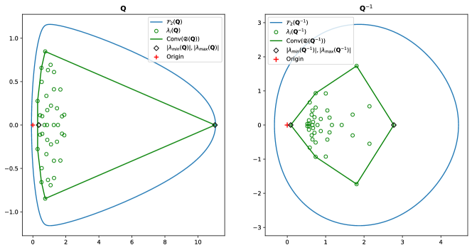
Figure 2: $2$-FoV boundary (blue line), eigenvalues (green circles), convex hull for eigenvalues (green line) and $|\lambda_{\text{min}}|,|\lambda_{\text{max}}|$ (black diamonds) for a matrix ${\bf Q}:={\bf I}+0.5\mathbf{E}\in\mathbb{R}^{40\times 40}$ (left) and its inverse ${\bf Q}^{-1}$ (right). $\mathbf{E}$ is a random matrix with $\mathbf{E}_{i,j}$ uniformly distributed random numbers in $[0,1]$ for $0\leq i,j\leq 40$. Remark that $0\neq\textup{Conv}(\mathfrak{S}({\bf Q}))$ (resp. $0\neq\textup{Conv}(\mathfrak{S}({\bf Q}^{-1}))$) while $0\in\mathcal{F}_{2}({\bf Q})$ (resp. $0\in\mathcal{F}_{2}({\bf Q}^{-1})$).

Figure 2 illustrates the above definitions for a random matrix. Remark that: (i) ${\bf Q}$ is invertible, as $|\lambda_{\text{min}}({\bf Q})|>0$; (ii) $\mathcal{F}_{2}({\bf Q})\not\subset\textup{Conv}(\mathfrak{S}({\bf Q}))$ and $\mathcal{F}_{2}({\bf Q}^{-1})\not\subset\textup{Conv}(\mathfrak{S}({\bf Q}^{-1}))$; (iii) $\text{Conv}(\mathfrak{\mathfrak{S}({\bf Q}}))$ and $\text{Conv}(\mathfrak{S}({\bf Q}^{-1}))$ are bounded away from the origin, whereas $0\in\mathcal{F}_{2}({\bf Q})$ and $0\in\mathcal{F}_{2}({\bf Q}^{-1})$. Moreover, one has $\kappa_{S}({\bf Q})=30.6$ while $\kappa_{2}({\bf Q})=58.3$, evidencing the non-normality of ${\bf Q}$.

5.2 General linear convergence estimates for GMRES$(m)$

Following [36, Chapter 5], let us recall the application of the weighted (resp. Euclidean) GMRES to a linear system ${\bf Q}{\bf x}={\bf d}$ in $\mathbb{C}^{N}$, where ${\bf Q}\in\mathbb{C}^{N\times N}$ is a complex nonsingular matrix. For an initial guess ${\bf x}_{0}\neq{\bf x}$, we introduce the residual ${\bf r}_{0}={\bf d}-{\bf Q}{\bf x}_{0}$ such that ${\bf r}_{0}\neq 0$ as well as Krylov spaces

$$\mathcal{K}^{k}({\bf Q},{\bf r}_{0}):=\textup{span}\{{\bf Q}^{j}{\bf r}_{0}:j=0,\ldots,k-1\},\quad 1\leq k\leq N.$$ (50)

For any step $1\leq k\leq N$, we define ${\bf x}_{k}$ and $\tilde{{\bf x}}_{k}$ to be the unique elements of $\mathcal{K}^{k}({\bf Q},{\bf r}_{0})$ satisfying the minimal residual property under the energy and Euclidean norms:

$$\begin{split}{\|{\bf r}_{k}\|}_{H}&:={\|{\bf d}-{\bf Q}{\bf x}_{k}\|}_{H}=\min_{{\bf x}\in\mathcal{K}^{k}({\bf Q},{\bf r}_{0})}{\|{\bf d}-{\bf Q}{\bf x}\|}_{H},\\ {\|\tilde{{\bf r}}_{k}\|}_{2}&:={\|{\bf d}-{\bf Q}\tilde{{\bf x}}_{k}\|}_{2}=\min_{{\bf x}\in\mathcal{K}^{k}({\bf Q},{\bf r}_{0})}{\|{\bf d}-{\bf Q}{\bf x}\|}_{2},\end{split}$$ (51)

respectively. We refer to either weighted or Euclidean GMRES collectively as GMRES. We add an $(m)$ superscript to signal restarted GMRES$(m)$, for any natural number $1\leq m\leq N$. Notice that GMRES and GMRES$(m)$ coincide up to iteration $m$.

Lemma 4 (Weighted GMRES$(m$): Linear bounds).

Let ${\bf Q}\in\mathbb{C}^{N\times N}$, with $0\neq\mathcal{F}_{H}({\bf Q})$ in (48) and set $1\leq m\leq N$. Then, the $k$-th residual of weighted GMRES$(m)$ for $1\leq k\leq N$ satisfies:

$$\frac{{\|{\bf r}_{k}\|}_{H}}{{\|{\bf r}_{0}\|}_{H}}\leq\left(1-\mathcal{V}_{H}({\bf Q})\mathcal{V}_{H}\left({\bf Q}^{-1}\right)\right)^{\frac{k}{2}}.$$ (52)

Proof.

We first remark that Lemma 4 for the Euclidean GMRES, i.e. for ${\bf H}={\bf I}$, is proved in [18]. Thus, we focus on the extension to weighted GMRES. Following [36, Theorem 5.1], we set $\widehat{{\bf Q}}:={\bf H}^{\frac{1}{2}}{\bf Q}{\bf H}^{-\frac{1}{2}}$, $\widehat{{\bf d}}:={\bf H}^{\frac{1}{2}}{\bf d}$, $\widehat{{\bf x}}:={\bf H}^{\frac{1}{2}}{\bf x}$ and $\widehat{{\bf r}}_{0}:={\bf H}^{\frac{1}{2}}{\bf r}_{0}$. Application of the Euclidean GMRES to $\widehat{{\bf Q}}\widehat{{\bf x}}=\widehat{{\bf d}}$ yields

$$\frac{{\|\widehat{{\bf r}}_{k}\|}_{2}}{{\|\widehat{{\bf r}}_{0}\|}_{2}}\leq\left(1-\mathcal{V}_{2}(\widehat{{\bf Q}})\mathcal{V}_{2}(\widehat{{\bf Q}}^{-1})\right)^{\frac{k}{2}}.$$ (53)

By Lemma 3, we obtain that $\mathcal{F}_{H}({\bf Q})=\mathcal{F}_{2}(\widehat{{\bf Q}})$ and $\mathcal{F}_{H}({\bf Q}^{-1})=\mathcal{F}_{2}({\bf H}^{1/2}{\bf Q}^{-1}{\bf H}^{-1/2})=\mathcal{F}_{2}(\widehat{{\bf Q}}^{-1})$. Consequently, by (53) we derive the final bound for the weighted GMRES

$$\frac{{\|{\bf r}_{k}\|}_{H}}{{\|{\bf r}_{0}\|}_{H}}\leq\left(1-\mathcal{V}_{H}({\bf Q})\mathcal{V}_{H}({\bf Q}^{-1})\right)^{\frac{k}{2}}=\rho^{k},$$ (54)

with $\rho:=\left(1-\mathcal{V}_{H}({\bf Q})\mathcal{V}_{H}({\bf Q}^{-1})\right)^{\frac{1}{2}}$ and $\rho<1$ by [18, Section 1]. Finally, we remark that $\rho$ above does not depend on $k$: it provides a one-step bound. Therefore, we set a restart $1\leq m\leq N$ and define $k=:im+t$ with $0\leq t<m$ and $0\leq i\leq\lfloor\frac{N}{m}\rfloor$. By application of (54), there holds that:

$${\|{\bf r}_{im+t}\|}_{H}\leq\rho^{t}{\|{\bf r}_{im}\|}_{H},$$ (55)

and thus, ${\|{\bf r}_{k}\|}_{H}\leq\rho^{k}{\|{\bf r}_{0}\|}_{H}$, leading to the expected result for GMRES$(m)$. ∎

Remark 8.

Lemma 4 provides a linear convergence bound for weighted GMRES$(m)$ with respect to $\mathcal{V}_{H}({\bf Q})$ and $\mathcal{V}_{H}({\bf Q}^{-1})$ and constitutes a sharper version of the classic result for weighted GMRES in [36, 6]. Indeed, for ${\bf Q}$ in Lemma 4 there holds that [18, Section 1]:

$$1-\mathcal{V}_{H}({\bf Q})\mathcal{V}_{H}({\bf Q}^{-1})\leq 1-\frac{\mathcal{V}_{H}({\bf Q})^{2}}{\|{\bf Q}\|_{H}^{2}}<1.$$

5.3 Discrete $\langle X_{h}\rangle$- and $(X_{h})$-coercivity

For the ensuing GMRES analysis of our preconditioned problem (​(CA)​), we need precise definitions for coercivity that relate to the BNB condition for Hilbert spaces. We introduce the notion of (discrete) $\langle X_{h}\rangle$-coercivity, with angle brackets referring to the dual pairing in (5) (refer to [50, Section 5]).

Definition 2 ($\langle X_{h}\rangle$-coercivity).

Consider $\mathsf{A}:X\to X^{\prime}$ as in the BG case with $X$ being a Hilbert space. For $h>0$ given, $\mathsf{A}$ is said to be $\langle X_{h}\rangle$-coercive if there exists $\alpha_{\mathsf{A}}$ such that

$$0<\alpha_{\mathsf{A}}\leq\frac{|\mathsf{a}(u_{h},u_{h})|}{{\|u_{h}\|}_{X}^{2}}=\frac{|\langle\mathsf{A}u_{h},u_{h}\rangle_{X^{\prime}\times X}|}{{\|u_{h}\|}_{X}^{2}}\quad\forall\ u_{h}\in X_{h}\setminus\{\boldsymbol{0}\}.$$ (56)

Thus, discrete $\langle X_{h}\rangle$-ellipticity refers to self-adjoint operators satisfying the $\langle X_{h}\rangle$-coercivity condition. These definitions extend naturally to continuous $\langle X\rangle$-coercivity and -ellipticity.

Remark 9 (BNB condition and $\langle X_{h}\rangle$-coercivity).

As pointed out for $\langle X\rangle$-coercivity in [2, Lemma 2.8] , $\langle X_{h}\rangle$-coercivity for $\mathsf{A}$ in Definition 2 provides a BNB constant $\gamma_{\mathsf{A}}=\alpha_{\mathsf{A}}$, since for any $u_{h}\in X_{h}\setminus\{\boldsymbol{0}\}$, it holds that

$$0<\alpha_{\mathsf{A}}{\|u_{h}\|}_{X}\leq\frac{|\mathsf{a}(u_{h},u_{h})|}{{\|u_{h}\|}_{X}}\leq\sup_{v_{h}\in X_{h}\setminus\{\boldsymbol{0}\}}\frac{|\mathsf{a}(u_{h},v_{h})|}{{\|v_{h}\|}_{X}}.$$ (57)

Remark 10.

$\langle X_{h}\rangle$-coercivity is a common property for BG methods in Hilbert spaces. For example, under suitable assumptions on the discretization scheme, operators with a Gårding inequality on $X$—of the form $\mathsf{A}=\mathsf{A}_{0}+\mathsf{K}:X\to X^{\prime}$ with $\mathsf{A}_{0}$ $\langle X\rangle$-coercive and $\mathsf{K}$ compact [41, Section 2.1]— admit a $h_{0}>0$ such that $\mathsf{A}$ is $\langle X_{h}\rangle$-coercive for all $0<h\leq h_{0}$ [41, Section 4.2.3].

Similarly to Definition 2, we introduce the discrete $(X_{h})$-coercivity, the difference being the use of inner products.

Definition 3 ($(X_{h})$-coercivity).

Consider $\mathsf{A}:X\to X$ for the PGE case with $X=:H$ being a Hilbert space. $\mathsf{A}$ is said to be $(X_{h})$-coercive if, for any $u_{h}\in X_{h}\setminus\{\boldsymbol{0}\}$, there exists $\alpha_{\mathsf{A}}>0$ such that

$$\alpha_{\mathsf{A}}\leq\frac{\left|(\mathsf{A}u_{h},u_{h})_{H}\right|}{(u_{h},u_{h})_{H}},$$ (58)

or equivalently

$$\alpha_{\mathsf{A}}\leq\inf_{u_{h}\in X_{h}\setminus\{\boldsymbol{0}\}}\frac{\left|(\mathsf{A}u_{h},u_{h})_{H}\right|}{(u_{h},u_{h})_{H}}=\mathcal{V}_{H}(\mathsf{A}_{h}).$$ (59)

Definition 3 via (59) shows the strong connection between $(X_{h})$-coercivity and discrete $\mathcal{V}_{H}$. Furthermore, under the OP setting, the discrete and matrix $H$-FoVs coincide.

Lemma 5.

Consider (​(CA)​) with $X=:H$ a Hilbert space with inner product $(\cdot,\cdot)_{H}$. There holds that

1. $\mathcal{F}_{H}(\mathsf{P}_{h}\mathsf{A}_{h})=\mathcal{F}_{H}({\bf P}{\bf A})$ and $\mathcal{F}_{H}((\mathsf{P}_{h}\mathsf{A}_{h})^{-1})=\mathcal{F}_{H}(({\bf P}{\bf A})^{-1})$;

2. $\mathcal{V}_{H}(\mathsf{P}_{h}\mathsf{A}_{h})=\mathcal{V}_{H}({\bf P}{\bf A})$ and $\mathcal{V}_{H}((\mathsf{P}_{h}\mathsf{A}_{h})^{-1})=\mathcal{V}_{H}(({\bf P}{\bf A})^{-1})$.

Proof.

Following (35), $q_{h}:=\mathsf{P}_{h}\mathsf{A}_{h}u_{h}\in X_{h}$ for any $u_{h}\in X_{h}$ has basis expansion ${\bf q}={\bf P}{\bf A}{\bf u}$. Therefore, there holds by (47) that for any $u_{h}\in X_{h}$:

$$(\mathsf{P}_{h}\mathsf{A}_{h}u_{h},u_{h})_{H}=({\bf P}{\bf A}{\bf u},{\bf u})_{H}\quad\text{and}\quad(u_{h},u_{h})_{H}=({\bf u},{\bf u})_{H},$$ (60)

yielding $\mathcal{F}_{H}(\mathsf{P}_{h}\mathsf{A}_{h})=\mathcal{F}_{H}({\bf P}{\bf A})$, and thus the expected result for $\mathsf{P}_{h}\mathsf{A}_{h}$. Similarly, one deduces the same result for the inverse operator since for any $q_{h}\in X_{h}$, $(\mathsf{P}_{h}\mathsf{A}_{h})^{-1}q_{h}$ has basis expansion $({\bf P}{\bf A})^{-1}{\bf q}$.∎

5.4 Linear convergence estimates for GMRES$(m)$ applied to (​(CA)​)

Following Section 5.2, application of the weighted (resp. Euclidean) preconditioned GMRES$(m)$, for $1\leq m\leq N$, to (​(CA)​)_μ,ν and initial guess ${\bf x}_{0}\neq{\bf u}_{\nu}$, produces the iterates ${\bf x}_{k}$ (resp. $\tilde{{\bf x}}_{k}$) for any step $1\leq k\leq N$ with minimal residual properties:

$$\begin{split}{\|{\bf P}_{\mu}{\bf r}_{k}\|}_{H}&:={\|{\bf P}_{\mu}{\bf b}_{\nu}-{\bf P}_{\mu}{\bf A}_{\nu}{\bf x}_{k}\|}_{H}=\min_{{\bf x}\in\mathcal{K}^{k}({\bf P}_{\mu}{\bf A}_{\nu},{\bf r}_{0})}{\|{\bf P}_{\mu}{\bf b}_{\nu}-{\bf P}_{\mu}{\bf A}_{\nu}{\bf x}\|}_{H},\\ {\|{\bf P}_{\mu}\tilde{{\bf r}}_{k}\|}_{2}&:={\|{\bf P}_{\mu}{\bf b}_{\nu}-{\bf P}_{\mu}{\bf A}_{\nu}\tilde{{\bf x}}_{k}\|}_{2}=\min_{{\bf x}\in\mathcal{K}^{k}\left({\bf P}_{\mu}{\bf A}_{\nu},{\bf r}_{0}\right)}{\|{\bf P}_{\mu}{\bf b}_{\nu}-{\bf P}_{\mu}{\bf A}_{\nu}{\bf x}\|}_{2},\end{split}$$ (61)

with $\mathcal{K}^{k}$ introduced in (50) and obvious construction for (​(CA)​). By (61), the minimal residuals satisfy

$${\|{\bf P}_{\mu}\tilde{{\bf r}}_{k}\|}_{2}\leq{\|{\bf P}_{\mu}{\bf r}_{k}\|}_{2}\quad\text{and}\quad{\|{\bf P}_{\mu}{\bf r}_{k}\|}_{H}\leq{\|{\bf P}_{\mu}\tilde{{\bf r}}_{k}\|}_{H}.$$ (62)

We set convergence rates for the weighted (resp. Euclidean) preconditioned GMRES$(m)$:

$$\Theta^{(m)}_{k}:=\left(\frac{{\|{\bf P}_{\mu}{\bf r}_{k}\|}_{H}}{{\|{\bf P}_{\mu}{\bf r}_{0}\|}_{H}}\right)^{\frac{1}{k}}\quad\text{and}\quad\widetilde{\Theta}_{k}^{(m)}:=\left(\frac{{\|{\bf P}_{\mu}\tilde{{\bf r}}_{k}\|}_{2}}{{\|{\bf P}_{\mu}{\bf r}_{0}\|}_{2}}\right)^{\frac{1}{k}}.$$ (63)

Finally, we define convergence rates for non-restarted weighted (resp. Euclidean) preconditioned GMRES $\Theta_{k}:=\Theta_{k}^{(N)}$ (resp. $\widetilde{\Theta}_{k}:=\widetilde{\Theta}_{k}^{(N)}$).

The bounds in Theorem 1 and Theorem 2 are related to the spectral radius, and rely on the continuity and discrete inf-sup constants: they do not supply information on the eigenvalue or FoV distributions, as pointed out in Figure 2, which are required to derive convergence results for iterative solvers to (​(CA)​)or (​(CA)​)_μ,ν. Thus, more specific conditions are required. For instance, for (​(CA)​) we enforce the following $(X_{h})$-coercivity condition for $\mathsf{P}_{h}\mathsf{A}_{h}$.

Assumption 3 ($(X_{h})$-coercivity for (​(CA)​)).

For problem (​(CA)​) with $X:=H$ being a Hilbert space with inner product $(\cdot,\cdot)_{H}$, we assume that $\mathsf{P}_{h}\mathsf{A}_{h}$ and its inverse are $(X_{h})$-coercive satisfying

$$\frac{\gamma_{\mathsf{C}}\gamma_{\mathsf{A}}}{\|\mathsf{m}\|\|\mathsf{n}\|}\leq\mathcal{V}_{H}(\mathsf{P}_{h}\mathsf{A}_{h})\quad\text{and}\quad\frac{\gamma_{\mathsf{M}}\gamma_{\mathsf{N}}}{\|\mathsf{c}\|\|\mathsf{a}\|}\leq\mathcal{V}_{H}((\mathsf{P}_{h}\mathsf{A}_{h})^{-1}).$$ (64)

Remark 11.

The $(X_{h})$-coercivity constants in 3 emerge naturally, as they are related to the BNB constants for both $\mathsf{P}_{h}\mathsf{A}_{h}$ and its inverse (cf. proof of Theorem 1). Alternatively, one can write 3 as:

$$0<\Gamma_{0}\leq\mathcal{V}_{H}(\mathsf{P}_{h}\mathsf{A}_{h})\quad\text{and}\quad 0<\Gamma_{1}\leq\mathcal{V}_{H}((\mathsf{P}_{h}\mathsf{A}_{h})^{-1}),$$ (65)

with $\Gamma_{0},\Gamma_{1}$ constants depending on the discrete inf-sup and continuity constants for the induced operators and eventually for $(\cdot,\cdot)_{H}$ in (47).

We are ready to state the linear convergence result for GMRES$(m)$ for (​(CA)​) for the Hilbertian case.

Theorem 3 (GMRES$(m)$: Linear convergence estimates for (​(CA)​)).

Consider (​(CA)​) with $X=:H$ Hilbert and $(\cdot,\cdot)_{H}$ such that 3 holds. Then, GMRES($m$) for $1\leq k,m\leq N$ leads to

$$\Theta_{k}^{(m)}\leq\left(1-\frac{1}{\operatorname{K}_{\star}}\right)^{\frac{1}{2}}\quad\textup{and}\quad\widetilde{\Theta}_{k}^{(m)}\leq\operatorname{K}_{\Lambda_{h}}\left(1-\frac{1}{\operatorname{K}_{\star}}\right)^{\frac{1}{2}},$$ (66)

with $\operatorname{K}_{\star}$ as defined in (36) and $\operatorname{K}_{\Lambda_{h}}$ in (16).

Proof.

By combining 3, Lemma 5 and definition of $\operatorname{K}_{\star}$, there holds that

$$\mathcal{V}_{H}({\bf P}{\bf A})\mathcal{V}_{H}(({\bf P}{\bf A})^{-1})\geq\frac{1}{\operatorname{K}_{\star}}$$ (67)

and thus

$$1-\mathcal{V}_{H}({\bf P}{\bf A})\mathcal{V}_{H}(({\bf P}{\bf A})^{-1})\leq 1-\frac{1}{\operatorname{K}_{\star}}$$

Application of Lemma 4 to the preconditioned system with residuals (61) provides the first bound in (66), namely

$$\frac{{\|{\bf P}{\bf r}_{k}\|}_{H}}{{\|{\bf P}{\bf r}_{0}\|}_{H}}\leq\left(1-\frac{1}{\operatorname{K}_{\star}}\right)^{\frac{k}{2}},\quad 1\leq k\leq N.$$ (68)

Next, we follow the steps in [6, Section 4] to arrive at the second bound in (66). First, the minimal residual property (62) yields

$${\|{\bf P}\tilde{{\bf r}}_{k}\|}_{2}\leq{\|{\bf P}{\bf r}_{k}\|}_{2}.$$ (69)

By virtue of the synthesis operator in (14), one has

$${\|{\bf P}{\bf r}_{k}\|}_{2}\leq\frac{1}{\gamma_{\Lambda_{h}}}{\|{\bf P}{\bf r}_{k}\|}_{H}\quad\text{and}\quad{\|{\bf P}{\bf r}_{0}\|}_{H}\leq\|\Lambda_{h}\|{\|{\bf P}{\bf r}_{0}\|}_{2}.$$ (70)

Therefore, (68) combined with (69) and (70) lead to the final result, as

$${\|{\bf P}\tilde{{\bf r}}_{k}\|}_{2}\leq{\|{\bf P}{\bf r}_{k}\|}_{2}\leq\frac{1}{\gamma_{\Lambda_{h}}}{\|{\bf P}{\bf r}_{k}\|}_{H}\leq\frac{1}{\gamma_{\Lambda_{h}}}\left(1-\frac{1}{\operatorname{K}_{\star}}\right)^{\frac{k}{2}}{\|{\bf P}{\bf r}_{0}\|}_{H}\leq\operatorname{K}_{\Lambda_{h}}\left(1-\frac{1}{\operatorname{K}_{\star}}\right)^{\frac{k}{2}}{\|{\bf P}{\bf r}_{0}\|}_{2},$$

as stated. ∎

Remark 12.

This result provides extensive convergence bounds for GMRES$(m)$. It will guarantee $h$-independent convergence for weighted GMRES$(m)$ for (​(CA)​) in the Hilbert setting (cf. Corollary 3). Also, the synthesis operator enters as an offset factor in $\widetilde{\Theta}_{k}^{(m)}=\operatorname{K}_{\Lambda_{h}}\rho$ with $\rho:=(1-1/\operatorname{K}_{\star})^{1/2}<1$. One should observe that $\widetilde{\Theta}_{k}^{(\text{m})}$ could be larger than 1 for $\operatorname{K}_{\Lambda_{h}}>1$, an impractical bound for Euclidean GMRES$(m)$. The latter supports theoretically the use of weighted GMRES$(m)$ as a solver [38].

To illustrate the application of the above results, we provide a case of interest where 3 is satisfied. Therein, notice the extra $\mathsf{K}_{\mathsf{A}}$-term in (71) below, justifying Remark 11.

Corollary 1 (Preconditioner-induced norm [38, 17, 19]).

Consider (​(CA)​) for OP-BG for Hilbert spaces $X=:H$ and $V$, $\mathsf{A}$ being $\langle X_{h}\rangle$-coercive, and $\mathsf{C}$ being $\langle V_{h}\rangle$-elliptic, with $\gamma_{\mathsf{A}}:=\alpha_{\mathsf{A}}$ and $\gamma_{\mathsf{C}}:=\alpha_{\mathsf{C}}$. Then, $\mathsf{P}^{-1}$ is Hermitian and yields an inner product on $X_{h}$, denoted by $(\cdot,\cdot)_{P^{-1}}$, and

$$\frac{\gamma_{\mathsf{C}}\gamma_{\mathsf{A}}}{\|\mathsf{m}\|^{2}}\leq\mathcal{V}_{P^{-1}}(\mathsf{P}_{h}\mathsf{A}_{h})\quad\text{and}\quad\frac{\gamma_{\mathsf{M}}^{2}}{\|\mathsf{c}\|\|\mathsf{a}\|}\operatorname{K}_{\mathsf{A}}\leq\mathcal{V}_{P^{-1}}((\mathsf{P}_{h}\mathsf{A}_{h})^{-1}).$$ (71)

Proof.

First, notice that since $\mathsf{C}$ is $\langle V_{h}\rangle$-elliptic, ${\bf C}$ and ${\bf C}^{-1}$ are Hermitian positive definite. Therefore, we deduce that ${\bf P}={\bf M}^{-1}{\bf C}{\bf M}^{-H}={\bf P}^{H}$ and ${\bf P}^{-1}={\bf P}^{-H}$ are Hermitian positive definite. For any ${\bf u},{\bf v}\in\mathbb{C}^{N}\setminus\{\boldsymbol{0}\}$ and ${\bf w}:={\bf P}^{-1}{\bf v}$, one has

$$\mathcal{V}_{P^{-1}}(\mathsf{P}_{h}\mathsf{A}_{h})=\inf_{{\bf u}\in\mathbb{C}^{N}\setminus\{\boldsymbol{0}\}}\frac{|({\bf P}{\bf A}{\bf u},{\bf u})_{P^{-1}}|}{({\bf u},{\bf u})_{P^{-1}}}=\inf_{{\bf u}\in\mathbb{C}^{N}\setminus\{\boldsymbol{0}\}}\frac{|({\bf A}{\bf u},{\bf u})_{2}|}{|({\bf P}^{-1}{\bf u},{\bf u})_{2}|}$$

and

$$\quad\mathcal{V}_{P^{-1}}((\mathsf{P}_{h}\mathsf{A}_{h})^{-1})=\inf_{{\bf v}\in\mathbb{C}^{N}\setminus\{\boldsymbol{0}\}}\frac{|({\bf A}^{-1}{\bf P}^{-1}{\bf v},{\bf v})_{P^{-1}}|}{({\bf v},{\bf v})_{P^{-1}}}=\inf_{{\bf w}\in\mathbb{C}^{N}\setminus\{\boldsymbol{0}\}}\frac{|({\bf A}^{-1}{\bf w},{\bf w})_{2}|}{|({\bf P}{\bf w},{\bf w})_{2}|}.$$

Next, using Equations 2.61 and 2.62 in Kirby [19], we deduce that:

$$\gamma_{\mathsf{A}}\|u_{h}\|_{X}^{2}\leq|({\bf A}{\bf u},{\bf u})_{2}|\leq\|\mathsf{a}\|\|u_{h}\|_{X}^{2}\quad\text{and}\quad\frac{\gamma_{\mathsf{A}}}{\|\mathsf{a}\|}\|w_{h}\|_{X_{{h}}^{\prime}}^{2}\leq|({\bf A}^{-1}{\bf w},{\bf w})_{2}|\leq\|\mathsf{a}\|\|w_{h}\|_{X_{{h}}^{\prime}}^{2},$$ (72)

while for the preconditioner ${\bf P}$ one has by [8, Section 13.2] that

$$\frac{\gamma_{\mathsf{C}}}{\|\mathsf{m}\|^{2}}\|w_{h}\|_{X_{h}^{\prime}}^{2}\leq|({\bf P}{\bf w},{\bf w})_{2}|\leq\frac{\|\mathsf{c}\|}{\gamma_{\mathsf{M}}^{2}}\|w_{h}\|_{X_{{h}}^{\prime}}^{2}\quad\text{and}\quad\frac{\gamma_{\mathsf{M}}^{2}}{\|\mathsf{c}\|}\|u_{h}\|_{X}^{2}\leq|({\bf P}^{-1}{\bf u},{\bf u})_{2}|\leq\frac{\|\mathsf{m}\|^{2}}{\gamma_{\mathsf{C}}}\|u_{h}\|_{X}^{2}.$$ (73)

Therefore,

$$\frac{\gamma_{\mathsf{A}}\gamma_{\mathsf{C}}}{\|\mathsf{m}\|^{2}}\leq\frac{|({\bf A}{\bf u},{\bf u})_{2}|}{|({\bf P}^{-1}{\bf u},{\bf u})_{2}|}\quad\text{and}\quad\frac{\gamma_{\mathsf{A}}\gamma_{\mathsf{M}}^{2}}{\|\mathsf{a}\|^{2}\|\mathsf{c}\|}\leq\frac{|({\bf A}^{-1}{\bf w},{\bf w})_{2}|}{|({\bf P}{\bf w},{\bf w})_{2}|},$$ (74)

finalizing the proof. ∎

Corollary 2.

Consider (​(CA)​) for OP-BG for Hilbert spaces $X=:H$ and $V$, $\mathsf{A}$ being $\langle X_{h}\rangle$-coercive, and $\mathsf{C}$ being $\langle V_{h}\rangle$-elliptic. Then, GMRES$(m)$ for $1\leq k,m\leq N$ leads to

$$\Theta_{k}^{(m)}\leq\left(1-\frac{1}{\operatorname{K}_{\star}\operatorname{K}_{\mathsf{A}}}\right)\quad\text{and}\quad\widetilde{\Theta}_{k}^{(m)}\leq\operatorname{K}_{\Lambda_{h}}\left(1-\frac{1}{\operatorname{K}_{\star}\operatorname{K}_{\mathsf{A}}}\right)^{\frac{1}{2}},$$ (75)

with $\operatorname{K}_{\star}$ as defined in (36), $\operatorname{K}_{\Lambda_{h}}$ in (16) and $\operatorname{K}_{\mathsf{A}}$ in (12).

Remark 13.

The $\operatorname{K}_{\mathsf{A}}$-term in Corollary 1 and Corollary 2 is removed if $\mathsf{A}$ is $\langle X_{h}\rangle$-elliptic, since $\mathsf{A}^{-1}$ is $\langle X_{h}^{\prime}\rangle$-elliptic with constant $1/\|\mathsf{a}\|$ [8, Section 13.2].

5.5 Linear convergence estimates for GMRES$(m)$ applied to (​(CA)​)_μ,ν

As in Section 5.4, we give counterparts to 3 and Theorem 3 for the bi-parametric preconditioned problem (​(CA)​)_μ,ν.

Assumption 4 ($(X_{h})$-coercivity for (​(CA)​)_μ,ν).

For (​(CA)​)_μ,ν with $X:=H$ being a Hilbert space with inner product $(\cdot,\cdot)_{H}$, assume that there holds that

$$\frac{\gamma_{\mathsf{C}_{\mu}}\gamma_{\mathsf{A}_{\nu}}}{\|\mathsf{m}\|\|\mathsf{n}\|}\leq\mathcal{V}_{H}(\mathsf{P}_{h,\mu}\mathsf{A}_{h,\nu})\quad\text{and}\quad\frac{\gamma_{\mathsf{M}}\gamma_{\mathsf{N}}}{\|\mathsf{c}_{\mu}\|\|\mathsf{a}_{\nu}\|}\leq\mathcal{V}_{H}((\mathsf{P}_{h,\mu}\mathsf{A}_{h,\nu})^{-1}).$$ (76)

Remark 11 remains valid for 4. With this, we can extend Theorem 3 to (​(CA)​)_μ,ν.

Theorem 4 (GMRES$(m)$: Linear convergence estimates for (​(CA)​)_μ,ν).

Consider (​(CA)​)_μ,ν along with 4. Then, the residuals for GMRES($m$) for $1\leq k,m\leq N$ are bounded as

$$\Theta_{k}^{(m)}\leq\left(1-\frac{1}{\operatorname{K}_{\star,\mu,\nu}}\right)^{\frac{1}{2}}\quad\textup{and}\quad\widetilde{\Theta}_{k}^{(m)}\leq\operatorname{K}_{\Lambda_{h}}\left(1-\frac{1}{\operatorname{K}_{\star,\mu,\nu}}\right)^{\frac{1}{2}},$$ (77)

with $\operatorname{K}_{\star,\mu,\nu}$ and $\operatorname{K}_{\Lambda_{h}}$ defined in (44) and (16), respectively.

Proof.

The result follows by direct application of Theorem 3 to (​(CA)​)_μ,ν. ∎

Remark 14.

The above result gives a controlled convergence rate for GMRES$(m)$ with respect to bi-parametric $(\mu,\nu)$-perturbations. As in the discussion ensuing Theorem 2 and in order to illustrate its practical implications, assume that the best approximation error in Lemma 2 converges at a rate $\mathcal{O}(h^{r})$, $r>0$, and $\nu=\mathcal{O}(h^{r})$. Therefore, provided that $\mu=\mathcal{O}(1)$ guarantees a bounded $\operatorname{K}_{\star,\mu,\nu}$, the bounds in (77) ensure linear convergence for the weighted GMRES$(m)$ (resp. Euclidean GMRES$(m)$, for $\operatorname{K}_{\Lambda_{h}}<1$).

5.6 Compact and Carleman class operators

So far, we have focused on the linear convergence rates for GMRES($m$). Yet, it is know that in many situations the bound in Lemma 4 “may significantly overestimate the GMRES residual norms” [18]. To better understand this, we aim to improve bounds for the case of second-kind Fredholm operators, which are known to display super-linear convergence results for GMRES, i.e. the radius of convergence tends to zero as $k\to\infty$. To this end, we introduce the concept of Carleman class operators.

Again, assuming $H$ to be a separable Hilbert space, we introduce $\mathcal{C}(H)\equiv\mathcal{C}(H;H)$ the space of compact operators on $H$. Given $\mathsf{T}\in\mathcal{L}(H;H)$, we denote the ordered singular values of $\mathsf{T}$ as $\sigma_{j}(\mathsf{T}):=\{\inf{\|\mathsf{T}-\mathsf{T}_{i}\|}_{H}:\mathsf{T}_{i}:H\to H,\ \textup{rank}\mathsf{T}_{i}<j\}$. For any $k\geq 1$, the $k$th partial arithmetic mean for the singular values reads

$$\overline{\sigma}_{k}(\mathsf{K}):=\frac{1}{k}\sum_{j=1}^{k}\sigma_{j}(\mathsf{K}).$$ (78)

For $p>0$, a compact operator $\mathsf{K}\in\mathcal{C}(H)$ is said to belong to the Carleman class $\mathcal{C}^{p}(H)$ [51, Section XI.9] if it holds that

$${\left|\kern-1.07639pt\left|\kern-1.07639pt\left|\mathsf{K}\right|\kern-1.07639pt\right|\kern-1.07639pt\right|}_{p}=\|\sigma(\mathsf{K})\|_{p}:=\left(\sum_{i=1}^{\infty}{\sigma_{i}(\mathsf{K})}^{p}\right)^{1/p}<\infty.$$ (79)

Next, we say that $\mathsf{Q}$ is a $p$-class Fredholm operator of the second-kind, $\mathsf{Q}\in\mathcal{F}\mathcal{C}^{p}(H)$ if and only if $\mathsf{Q}-\mathsf{I}\in\mathcal{C}(H)$ for $p=0$ (resp. $\mathsf{Q}-\mathsf{I}\in\mathcal{C}^{p}(H)$ for $p>0$). Consequently, for $H=:X$ a separable Hilbert space, $p\geq 0$ and $\nu,\mu\in[0,1)$, we define the following problems:

$$\textup{(\!(A)\!)}^{p}:\quad\textup{(\!(A)\!)}\quad\text{for PGE (i.e.~{}$\mathsf{A}:H\to H$) with }\mathsf{A}\in\mathcal{F}\mathcal{C}^{p}(H)\quad\text{and}\quad\mathsf{N}:=\mathsf{I},$$ (80)

and

$$\textup{(\!(CA)\!)}_{\mu,\nu}^{p}:\quad\textup{(\!(CA)\!)}_{\mu,\nu}\quad\text{with}\quad\mathsf{C}_{\mu}\mathsf{N}^{-1}\mathsf{A}_{\nu}\in\mathcal{F}\mathcal{C}^{p}(H),\quad\text{and}\quad\mathsf{M}:=\mathsf{I},$$ (81)

whose diagram representation is

$$\textup{{(\!(CA)\!)}}_{\mu,\nu}^{p}:\quad\leavevmode\hbox to65.41pt{\vbox to56.29pt{\text{[drawing]}}}. {H} {Y^{\prime}} {H} {V} \scriptstyle{\mathsf{A}_{\nu}} \scriptstyle{\mathsf{N}^{-1}} \scriptstyle{\mathsf{I}^{-1}} \scriptstyle{\mathsf{C}_{\mu}}$$

Finally, for (​(A)​)^p and (​(CA)​)${}^{p}_{\mu,\nu}$, the corresponding compact terms $\mathsf{K}:=\mathsf{A}-\mathsf{I}$ and $\mathsf{K}_{\mu,\nu}:=\mathsf{C}_{\mu}\mathsf{N}^{-1}\mathsf{A}_{\nu}-\mathsf{I}$ have discrete counterparts $\mathsf{K}_{h}:=\mathsf{A}_{h}-\mathsf{I}_{h}$ and $\mathsf{K}_{h,\mu,\nu}:=\mathsf{C}_{h}\mathsf{N}_{h}^{-1}\mathsf{A}_{h}-\mathsf{I}_{h}$ with Galerkin matrices defined as

$${\bf K}:={\bf A}-{\bf N}\quad\text{and}\quad{\bf K}_{\mu,\nu}:={\bf C}_{\mu}{\bf N}^{-1}{\bf A}_{\nu}-{\bf M},$$ (82)

respectively. In the sequel, we introduce ordered (matrix) singular values with respect to the $H$-norm [33, Proposition 4.2]:

$$\sigma_{j}^{H}({\bf Q}):=\lambda_{j}({\bf Q}^{\star}{\bf Q})^{1/2}=\sigma_{j}({\bf H}^{1/2}{\bf Q}{\bf H}^{-1/2}),$$ (83)

for any ${\bf Q}\in\mathbb{C}^{N\times N}$ and ${\bf Q}^{\star}={\bf H}^{-1}{\bf Q}^{H}{\bf H}$ its $H$-adjoint.

5.7 Super-linear convergence estimates for GMRES applied to (​(A)​)^p

We recall the classic super-linear convergence result for weighted GMRES on a (continuous) Hilbert setting level (cf. [20] and [33, Theorem 3.1]).

Proposition 3 (Weighted GMRES: Classic super-linear convergence estimate [33, Theorem 3.1]).

Let $H$ be a Hilbert space. Set $p\geq 0$ and consider the application of weighted GMRES on $\mathsf{Q}x={f}$, for a bounded and invertible operator $\mathsf{Q}\in\mathcal{F}\mathcal{C}^{p}(H)$ with $f\in H$. Introduce GMRES iterates $x_{0}\neq x$, and $x_{k}$, along with $r_{k}:=\mathsf{Q}x_{k}-f$, for any $k\geq 1$. Then, the residuals satisfy

$$\left(\frac{{\|r_{k}\|}_{H}}{{\|r_{0}\|}_{H}}\right)^{\frac{1}{k}}\leq{\|\mathsf{Q}^{-1}\|}_{H}\overline{\sigma}_{k}(\mathsf{K}),$$

wherein $\mathsf{K}:=\mathsf{Q}-\mathsf{I}\in\mathcal{C}(H)$ for $p=0$ (resp.  $\mathcal{C}^{p}(H)$ for $p>0$) and $\overline{\sigma}_{k}(\mathsf{K})$ defined in (78).

Remark that $\overline{\sigma}_{k}(\mathsf{K})\to 0$ as $k\to\infty$ evidencing the super-linear convergence rate for residuals of weighted GMRES in this particular case. Furthermore, the convergence rate depends directly on the singular values of the continuous operator $\mathsf{K}$. The following result shows that the above is applicable to (​(A)​)^p as well.

Theorem 5 (GMRES: Super-linear convergence estimates for (​(A)​)^p).

Consider the PGE problem (​(A)​)^p in (80) for any $p\geq 0$. Then, for $1\leq k\leq N$, it holds that

$$\left(\frac{{\|{\bf r}_{k}\|}_{H}}{{\|{\bf r}_{0}\|}_{H}}\right)^{\frac{1}{k}}\leq\frac{\overline{\sigma}_{k}(\mathsf{K})}{\gamma_{\mathsf{A}}\gamma_{\mathsf{N}}}\quad\left({\leq\frac{{\left|\kern-1.07639pt\left|\kern-1.07639pt\left|\mathsf{K}\right|\kern-1.07639pt\right|\kern-1.07639pt\right|}_{p}}{\gamma_{\mathsf{A}}\gamma_{\mathsf{N}}}k^{-\frac{1}{p}}}\quad\text{if}\quad p>0\right),$$ (84)

and

$$\left(\frac{{\|\tilde{{\bf r}}_{k}\|}_{2}}{{\|{\bf r}_{0}\|}_{2}}\right)^{\frac{1}{k}}\leq\operatorname{K}_{\Lambda_{h}}\frac{\overline{\sigma}_{k}(\mathsf{K})}{\gamma_{\mathsf{A}}\gamma_{\mathsf{N}}}\quad\left({\leq\operatorname{K}_{\Lambda_{h}}\frac{{\left|\kern-1.07639pt\left|\kern-1.07639pt\left|\mathsf{K}\right|\kern-1.07639pt\right|\kern-1.07639pt\right|}_{p}}{\gamma_{\mathsf{A}}\gamma_{\mathsf{N}}}}k^{-\frac{1}{p}}\quad\text{if}\quad p>0\right),$$ (85)

wherein $\mathsf{K}:=\mathsf{A}-\mathsf{I}\in\mathcal{C}(H)$ for $p=0$ (resp. $\mathcal{C}^{p}(H)$ for $p>0$) and $\overline{\sigma}_{k}(\mathsf{K})$ from (78).

Proof.

By hypothesis, we have that ${\bf N}^{-1}{\bf A}={\bf I}+{\bf N}^{-1}{\bf K}$, with ${\bf K}$ such as in (82). Following the same steps as in Axelsson [33], we deduce that the following relations hold (cf. proofs of Theorem 1 and Lemma 5):

$${\|({\bf N}^{-1}{\bf A})^{-1}\|}_{H}\leq\frac{\|\mathsf{n}\|}{\gamma_{\mathsf{A}}}\ =\frac{1}{\gamma_{\mathsf{A}}},$$

since $\mathsf{N}=\mathsf{I}$. Furthermore, it holds that the singular values [33, Proposition 4.2]

$$\sigma_{j}^{{H}}({\bf N}^{-1}{\bf K})\leq\frac{1}{\gamma_{\mathsf{N}}}\sigma_{j}(\mathsf{K}_{h})\leq\frac{1}{\gamma_{\mathsf{N}}}\sigma_{j}(\mathsf{K}).$$

Therefore, for $1\leq k\leq N$, following [33] and using Proposition 3, we can show that

$$\frac{{\|{\bf r}_{k}\|}_{H}}{{\|{\bf r}_{0}\|}_{H}} \leq\frac{{\|({\bf N}^{-1}{\bf A})^{-1}\|}_{H}}{k}\sum_{j=1}^{k}\sigma_{j}^{{H}}({\bf N}^{-1}{\bf K})\leq\frac{1}{\gamma_{\mathsf{A}}}\sum_{j=1}^{k}\frac{\sigma_{j}^{{H}}({\bf N}^{-1}{\bf K})}{k}\leq\frac{1}{\gamma_{\mathsf{A}}\gamma_{\mathsf{N}}}\sum_{j=1}^{k}\frac{\sigma_{j}(\mathsf{K})}{k}.$$

Now, if $\mathsf{K}\in\mathcal{C}^{p}(H)$ for any $p>0$, we follow [21, Theorem 2.2] and derive

$$\sum_{j=1}^{k}\frac{\sigma_{j}(\mathsf{K})}{k}\leq{\left|\kern-1.07639pt\left|\kern-1.07639pt\left|\mathsf{K}\right|\kern-1.07639pt\right|\kern-1.07639pt\right|}_{p}k^{-\frac{1}{p}},$$

providing the final estimate in energy norm.

Finally, the bounds in Euclidean norm are deduced in the same fashion as in Theorem 3. ∎

Remark 15.

This result appears to be new and it justifies the positive results of employing mass matrix preconditioning, i.e. $\mathsf{N}:=\mathsf{I}$, to transfer the super-linear convergence bounds from the continuous to the discrete level. Indeed, the choice of $\mathsf{N}=\mathsf{I}$ guarantees a discrete system ${\bf N}^{-1}{\bf A}={\bf I}+{\bf N}^{-1}{\bf K}$ of the form ${\bf I}$ plus discretization of a compact operator. The latter enables the application of the classical super-linear results for GMRES given in Proposition 3. Notice that the bounds in (84) and (85) depend on $k$ via $\overline{\sigma}_{k}(\mathsf{K})$: they are not one-step bounds, and do not generalize to GMRES$(m)$, as the relative error at iteration $k$ for $2\leq k\leq N$ depends on previous iterations.

Remark 16.

The super-linear convergence rate depends on the decay rate of $\overline{\sigma}_{k}(\mathsf{K})$. For example, for trace class operators ($p=1$), it holds that ${\|{\bf r}_{k}\|}_{H}/{\|{\bf r}_{0}\|}_{H}=\mathcal{O}(k^{-1})$ while for Hilbert-Schmidt operators ($p=2$), one observes the faster rate ${\|{\bf r}_{k}\|}_{H}/{\|{\bf r}_{0}\|}_{H}=\mathcal{O}(k^{-2})$ [51, Chapter XI]. Results describing the Carleman class index for pseudo-differential operators (resp. the Laplace double-layer operator) can be found in [52] (resp. [53, 54]) and will be investigated elsewhere.

5.8 Super-linear convergence estimates for GMRES applied to (​(CA)​)${}_{\mu,\nu}^{p}$

We next show that the reasoning in Theorem 5 can also be applied to (​(CA)​)${}^{p}_{\mu,\nu}$.

Theorem 6 (GMRES: Super-linear convergence estimates for (​(CA)​)${}_{\mu,\nu}^{p}$).

Consider (​(CA)​)${}^{p}_{\mu,\nu}$ in (81) for any $p\geq 0$ and define $\mathsf{K}_{\mu,\nu}:=\mathsf{C}_{\mu}\mathsf{N}^{-1}\mathsf{A}_{\nu}-\mathsf{I}\in\mathcal{C}(H)$ for $p=0$ (resp. $\mathcal{C}^{p}(H)$ for $p>0$). Then, for weighted and Euclidean GMRES, respectively, it holds that

$$\begin{split}\Theta_{k}&\leq\frac{\|\mathsf{n}\|}{\gamma_{\mathsf{C}}\gamma_{\mathsf{A}}\gamma_{\mathsf{M}}}\frac{\overline{\sigma}_{k}(\mathsf{K}_{\mu,\nu})}{(1-\mu)(1-\nu)}\quad\left(\leq\frac{\|\mathsf{n}\|}{\gamma_{\mathsf{C}}\gamma_{\mathsf{A}}\gamma_{\mathsf{M}}}\frac{{\left|\kern-1.07639pt\left|\kern-1.07639pt\left|\mathsf{K}_{\mu,\nu}\right|\kern-1.07639pt\right|\kern-1.07639pt\right|}_{p}}{(1-\mu)(1-\nu)}k^{-\frac{1}{p}}\quad\text{if}\quad p>0\right),\end{split}$$ (86)

and

$$\begin{split}\widetilde{\Theta}_{k}&\leq\operatorname{K}_{\Lambda_{h}}\frac{\|\mathsf{n}\|}{\gamma_{\mathsf{C}}\gamma_{\mathsf{A}}\gamma_{\mathsf{M}}}\frac{\overline{\sigma}_{k}(\mathsf{K}_{\mu,\nu})}{(1-\mu)(1-\nu)}\quad\left(\leq\operatorname{K}_{\Lambda_{h}}\frac{\|\mathsf{n}\|}{\gamma_{\mathsf{C}}\gamma_{\mathsf{A}}\gamma_{\mathsf{M}}}\frac{{\left|\kern-1.07639pt\left|\kern-1.07639pt\left|\mathsf{K}_{\mu,\nu}\right|\kern-1.07639pt\right|\kern-1.07639pt\right|}_{p}}{(1-\mu)(1-\nu)}k^{-\frac{1}{p}}\quad\text{if}\quad p>0\right),\end{split}$$ (87)

with ${\Theta}_{k}$ and $\widetilde{\Theta}_{k}$ defined in (63) and $\overline{\sigma}_{k}(\cdot)$ in (78).

Proof.

Consider (​(CA)​)${}^{p}_{\mu,\nu}$ and follow the proof of Theorem 5. First, we use Proposition 1 to deduce that

$${\|({\bf P}_{\mu}{\bf A}_{\nu})^{-1}\|}_{H}={{\|{\bf A}^{-1}_{\nu}{\bf N}{\bf C}^{-1}_{\mu}{\bf M}\|}_{H}}\leq\frac{\|\mathsf{n}\|}{\gamma_{\mathsf{A}}\gamma_{\mathsf{C}}}\frac{1}{(1-\mu)(1-\nu)}.$$

Next, for $1\leq j\leq N$, one has

$$\sigma_{j}^{{H}}({\bf M}^{-1}{\bf C}_{\mu}{\bf N}^{-1}{\bf A}_{\nu}-{\bf I})={\sigma_{j}^{{H}}({\bf M}^{-1}{\bf K}_{\mu,\nu})}\leq\frac{1}{\gamma_{\mathsf{M}}}\sigma_{j}(\mathsf{K}_{\mu,\nu}),$$

with ${\bf K}_{\mu,\nu}={\bf C}_{\mu}{\bf N}^{-1}{\bf A}-{\bf M}$ as in (82). Therefore, we obtain

$$\Theta_{k} \leq\frac{{\|({\bf P}_{\mu}{\bf A}_{\nu})^{-1}\|}_{H}}{k}\sum_{j=1}^{k}\sigma_{j}^{{H}}({\bf M}^{-1}{\bf K}_{\mu,\nu})\leq\frac{\|\mathsf{n}\|}{\gamma_{\mathsf{C}}\gamma_{\mathsf{A}}\gamma_{\mathsf{M}}}\frac{\overline{\sigma}_{k}(\mathsf{K}_{\mu,\nu})}{(1-\mu)(1-\nu)}.$$

The second bound in (86) and (87) follows by the same arguments as in the proof of Theorem 5. ∎

Theorem 6 describes precisely the residual convergence behavior of GMRES for (​(CA)​)${}^{p}_{\mu,\nu}$ for $p\geq 0$. In particular, (87) shows that the Euclidean GMRES converges super-linearly, up to a $\operatorname{K}_{\Lambda_{h}}$-term as observed experimentally for the electric field integral equation on screens in [35].

Corollary 3 ($h$-Asymptotics).

Consider (​(CA)​)_μ,ν in (77), for $\mu\to 0$ and $\nu\to 0$ as $h\to 0$. Additionally, let us suppose that (i) the finite dimensional subspaces are dense in their function space, satisfying the approximability property [2, Definition 2.14]; and, (ii) the forms in (​(CA)​) have a uniform discrete inf-sup condition with respect to $h$. Then, for vanishing $h$, the following statements hold:

1. $\|u-u_{h}\|_{X}\to 0$ in Lemma 2;

2. $\operatorname{K}_{\star}$ in Theorem 1, and subsequently $\operatorname{K}_{\star,\mu,\nu}$ Theorem 2 remain bounded ($h$-independence);

3. Under 4, the residual $\Theta_{k}^{(m)}$ in (77) remains bounded ($h$-independent linear convergence);

4. For (​(CA)​)${}^{p}_{\mu,\nu}$ in (81), $p\geq 0$, the residual $\Theta_{k}\to 0$ as $k\to\infty$ in Theorem 6 ($h$-independent super-linear convergence).

Remark 17.

Theorem 6 requires the operator $\mathsf{K}_{\mu,\nu}$ to be compact so as to ensure application of Proposition 3. Recent results by Bletcha [55] allow to consider a more general Proposition 3 with $\mathsf{A}:H\to H$ of the form $\mathsf{A}=\mathsf{Q}+\mathsf{K}$, with $\mathsf{Q}$ a bounded invertible operator and $\mathsf{K}$ compact. The latter could allow to relax the compactness for $\mathsf{K}_{\mu,\nu}$ and to analyze (​(CA)​)_μ,ν as a general bounded perturbation of (​(CA)​)^p. This will be investigated elsewhere.

5.9 Elliptic Case

We give further insight on the bi-parametric operator preconditioning framework by considering the elliptic case for OP-BG for $X=:H$ and $V$ being Hilbert spaces. To this end, we assume that $\mathsf{A}$ is $\langle X\rangle$-elliptic and $\mathsf{C}$ is $\langle V\rangle$-elliptic. Therefore, we have the ellipticity conditions

$$\mathsf{a}(u,u)\geq\alpha_{\mathsf{A}}{\|u\|}^{2}_{X}\quad\text{and}\quad\mathsf{c}(v,v)\geq\alpha_{\mathsf{C}}{\|v\|}^{2}_{V},$$

for all $u\in X$ and all $v\in V$. Notice that continuous ellipticity implies a discrete inf-sup condition for conforming discretization spaces, with $\gamma_{\mathsf{A}}=\alpha_{\mathsf{A}}$ and $\gamma_{\mathsf{C}}=\alpha_{\mathsf{C}}$, respectively, and allows to apply our previous analysis—without requiring 3.

For $p\geq 0$, problem (​(CA)​)^p leads to $\mathsf{C}\mathsf{N}^{-1}\mathsf{A}=\mathsf{I}+\mathsf{K}$ with $\mathsf{K}$ compact and self-adjoint. Thus, we introduce the ordered eigenvalues $|\lambda_{i+1}(\mathsf{K})|\leq|\lambda_{i}(\mathsf{K})|$ for $i\geq 1$. By [21, Section 2], $|\lambda_{i}(\mathsf{K})|=\sigma_{i}(\mathsf{K})$ and the Carleman class in (79) simplifies to the Neumann-Schatten class

$${\left|\kern-1.07639pt\left|\kern-1.07639pt\left|\mathsf{K}\right|\kern-1.07639pt\right|\kern-1.07639pt\right|}_{p}:=\left(\sum_{i=1}^{\infty}|\lambda_{i}(\mathsf{K})|\right)^{1/p}<\infty.$$ (88)

As ellipticity allows for more refined bounds, one can examine the use of preconditioned CG solvers [8, Section 13.1].

Corollary 4 (Elliptic Case).

Consider (​(CA)​)_μ,ν with $\mathsf{c}_{\mu}\in\Phi_{h,\mu}(\mathsf{c})$, $\mathsf{a}_{\nu}\in\Phi_{h,\nu}(\mathsf{a})$, such that $\mathsf{A}_{\nu}$ is $\langle X\rangle$-elliptic and $\mathsf{C}_{\mu}$ is $\langle V\rangle$-elliptic.Then, the continuous and perturbed problems have a unique solution, $u$ and $u_{h,\nu}$, respectively, with the following error bound

$${\|u-u_{h,\nu}\|}_{X} \leq\inf_{w_{h}\in X_{h}}\left(\frac{{\operatorname{K}_{\mathsf{A}}}}{1-\nu}\|u-w_{h}\|_{X}+\frac{\nu}{1-\nu}{\|w_{h}\|}_{X}\right)+\frac{\nu}{\gamma_{\mathsf{A}}(1-\nu)}{\|b_{{h}}\|}_{Y_{h}^{\prime}}$$

$${\leq\left(\frac{{\operatorname{K}_{\mathsf{A}}^{2}}}{1-\nu}\right)\inf_{w_{h}\in X_{h}}{\|u-w_{h}\|}_{X}+\frac{2\nu}{\gamma_{\mathsf{A}}(1-\nu)}{\|b_{{h}}\|}_{Y_{h}^{\prime}}.}$$

with $\operatorname{K}_{\mathsf{A}}$ defined in (12). Furthermore, it holds that

$$\kappa_{S}({\bf P}_{\mu}{\bf A}_{\nu})=\kappa_{2}({\bf P}_{\mu}{\bf A}_{\nu})\leq\operatorname{K}_{\star,\mu,\nu},$$ (89)

with $\operatorname{K}_{\star,\mu,\nu}$ in (45). Therefore, for ${\bf x}_{0}\neq{\bf u}_{\nu}$ and $1\leq k\leq N$, the $k$-th iterate ${\bf x}_{k}$ of CG with an error $\mathbf{e}_{k}:={\bf x}_{k}-{\bf u}_{\nu}$ is bounded in the $A_{\nu}$-norm as

$$\Theta_{k}^{\textup{CG}}:=\left(\frac{{\|\mathbf{e}_{k}\|}_{A_{\nu}}}{{\|\mathbf{e}_{0}\|}_{A_{\nu}}}\right)^{\frac{1}{k}}\leq 2^{\frac{1}{k}}\left(1-\frac{2}{\sqrt{\operatorname{K}_{\star,\mu,\nu}}+1}\right).$$ (90)

Finally, consider (​(CA)​)${}_{\mu,\nu}^{p}$ for $p\geq 0$. It holds that

$$\begin{split}\Theta_{k}^{\textup{CG}}&\leq\frac{2\|\mathsf{n}\|}{\gamma_{\mathsf{C}}\gamma_{\mathsf{A}}\gamma_{\mathsf{M}}}\frac{1}{(1-\mu)(1-\nu)}\cdot\frac{1}{k}\sum_{j=1}^{k}|\lambda_{j}(\mathsf{K}_{\mu,\nu})|\end{split}$$ (91)

and, if $p>0$, one retrieves

$$\begin{split}\Theta_{k}^{\textup{CG}}\leq\frac{2\|\mathsf{n}\|}{\gamma_{\mathsf{C}}\gamma_{\mathsf{A}}\gamma_{\mathsf{M}}}\frac{{\left|\kern-1.07639pt\left|\kern-1.07639pt\left|\mathsf{K}_{\mu,\nu}\right|\kern-1.07639pt\right|\kern-1.07639pt\right|}_{p}}{(1-\mu)(1-\nu)}k^{-\frac{1}{p}}.\end{split}$$ (92)

Proof.

By the ellipticity hypothesis on the sesqui-linear form $\mathsf{a}$, Lemma 1 is replaced by the Lax-Milgram lemma [2, Section 2.1.2], providing the sharper quasi-optimality constant ${\operatorname{K}_{\mathsf{A}}}$. Since the resulting system is Hermitian positive definite, the spectral and Euclidean condition numbers coincide. Next, we set $\varkappa:=\kappa_{S}({\bf P}_{\mu}{\bf A}_{\nu})$ and introduce the linear bound for the preconditioned CG with respect to the condition number [56, Theorem 1.8]:

$$\Theta_{k}^{\textup{CG}}\leq 2^{\frac{1}{k}}\left(\frac{\sqrt{\varkappa}-1}{\sqrt{\varkappa}+1}\right).$$ (93)

Observe that

$$\left(\frac{\sqrt{\varkappa}-1}{\sqrt{\varkappa}+1}\right)=\left(1-\frac{2}{\sqrt{\varkappa}+1}\right)\leq\left(1-\frac{2}{\sqrt{\operatorname{K}_{\star,\mu,\nu}}+1}\right),$$

leading to (90). Since, (​(CA)​)${}^{p}_{\mu,\nu}$ entails a self-adjoint compact perturbation $\mathsf{K}_{\mu,\nu}:=\mathsf{C}_{\mu}\mathsf{N}^{-1}\mathsf{A}_{\nu}-\mathsf{I}$, one has an ordered eigenvalue decomposition, and the application of super-linear result for CG [56, Theorem 1.9]:

$$\Theta_{k}^{\textup{CG}}\leq 2{\|({\bf P}_{\mu}{\bf A}_{\nu})^{-1}\|}_{H}\left(\frac{1}{k}\sum_{j=1}^{k}|\lambda_{j}({\bf M}^{-1}{\bf K}_{\mu,\nu})|\right).$$

Finally, one can show that (cf. proof of Theorem 6):

$${\|{\bf A}_{\nu}^{-1}{\bf P}_{\mu}^{-1}\|}_{H}\leq\frac{\|\mathsf{n}\|}{\gamma_{\mathsf{C}}\gamma_{\mathsf{A}}}\frac{1}{(1-\mu)(1-\nu)}\quad\text{and}\quad|\lambda_{j}({\bf M}^{-1}{\bf K}_{\mu,\nu})|\leq\frac{1}{\gamma_{\mathsf{M}}}|\lambda_{j}(\mathsf{K}_{\mu,\nu})|,$$

proving the final result. ∎

6 Conclusion

For general Petrov-Galerkin methods, we considered their operator preconditioning and introduced the novel bi-parametric framework. Several results were derived including bounds in Euclidean norm for the convergence of iterative solvers when preconditioning, with GMRES as a reference. These results pave the way toward new paradigms for preconditioning, as they allow to craft robust preconditioners, better understand the efficiency of existing ones and relate them to experimental results. We see direct applications in a variety of research areas including wave propagation problems [57], singular perturbation theory [32, Section 3], fast numerical methods [25, 46] and iterative solvers [4].

Future work avenues we foresee are: further analysis of second-kind Fredholm integral equations, with applications to acoustics and electromagnetics; deep learning of preconditioners for GMRES, and wavenumber asymptotic analysis for preconditioners. Also, we mention two promising research areas: (i) extension of (​(CA)​)${}_{\mu,\nu}^{p}$ to bounded perturbations of (​(CA)​)^p via [55]; and (ii) characterization of Carleman class for compact operators using elliptic regularity theorems [53].

References

- [1] T. Betcke, M. W. Scroggs, W. Śmigaj, Product algebras for Galerkin discretisations of boundary integral operators and their applications, ACM Transactions on Mathematical Software (TOMS) 46 (1) (2020) 1–22.
- [2] A. Ern, J. Guermond, Theory and Practice of Finite Elements, Applied Mathematical Sciences, Springer New York, 2004.
- [3] Y. Saad, Iterative Methods for Sparse Linear Systems, 2nd Edition, Society for Industrial and Applied Mathematics, USA, 2003.
- [4] Y. Saad, M. H. Schultz, GMRES: A Generalized Minimal Residual Algorithm for Solving Nonsymmetric Linear Systems, SIAM J. Sci. Stat. Comput. 7 (3) (1986) 856–869.
- [5] M. R. Hestenes, E. Stiefel, et al., Methods of conjugate gradients for solving linear systems, Journal of research of the National Bureau of Standards 49 (6) (1952) 409–436.
- [6] M. Sarkis, D. B. Szyld, Optimal left and right additive Schwarz preconditioning for minimal residual methods with Euclidean and energy norms, Computer Methods in Applied Mechanics and Engineering 196 (8) (2007) 1612–1621.
- [7] B. Beckermann, S. A. Goreinov, E. E. Tyrtyshnikov, Some Remarks on the Elman estimate for GMRES, SIAM Journal on Matrix Analysis and Applications 27 (3) (2005) 772–778.
- [8] O. Steinbach, Numerical Approximation Methods for Elliptic Boundary Value Problems: Finite and Boundary Elements, Texts in Applied Mathematics, Springer New York, 2007.
- [9] O. Nevanlinna, Convergence of Iterations for Linear Equations, Birkhauser Verlag, CHE, 1993.
- [10] R. Hiptmair, Operator Preconditioning, Computers and Mathematics with Applications 52 (5) (2006) 699–706.
- [11] S. H. Christiansen, J.-C. Nédélec, Des préconditionneurs pour la résolution numérique des équations intégrales de frontière de l’acoustique, Comptes Rendus de l’Académie des Sciences-Series I-Mathematics 330 (7) (2000) 617–622.
- [12] R. Andreev, Stability of sparse space-time finite element discretizations of linear parabolic evolution equations, IMA Journal of Numerical Analysis 33 (1) (2013) 242–260.
- [13] O. Steinbach, W. L. Wendland, The construction of some efficient preconditioners in the boundary element method, Advances in Computational Mathematics 9 (1-2) (1998) 191–216.
- [14] W. McLean, O. Steinbach, Boundary element preconditioners for a hypersingular integral equation on an interval, Advances in Computational Mathematics 11 (4) (1999) 271–286.
- [15] G. C. Hsiao, W. L. Wendland, Boundary Integral Equations, Springer Berlin Heidelberg, 2008.
- [16] R. Stevenson, R. van Venetië, Uniform Preconditioners of Linear complexity for Problems of Negative Order, Computational Methods in Applied Mathematics 21 (2) (2021) 469–478.
- [17] G. Starke, Field-of-values analysis of preconditioned iterative methods for nonsymmetric elliptic problems, Numerische Mathematik 78 (1) (1997) 103–117.
- [18] J. Liesen, P. Tichý, The field of values bound on ideal GMRES, arXiv preprint arXiv:1211.5969 (2012).
- [19] R. C. Kirby, From Functional Analysis to Iterative Methods, SIAM Review 52 (2) (2010) 269–293.
- [20] I. Moret, A note on the superlinear convergence of GMRES, SIAM Journal on Numerical Analysis 34 (2) (1997) 513–516.
- [21] R. Winther, Some superlinear convergence results for the conjugate gradient method, SIAM Journal on Numerical Analysis 17 (1) (1980) 14–17.
- [22] S. L. Campbell, I. C. Ipsen, C. T. Kelley, C. D. Meyer, GMRES and the minimal polynomial, BIT Numerical Mathematics 36 (4) (1996) 664–675.
- [23] O. Axelsson, J. Karátson, Superlinear convergence of the GMRES for PDE-constrained optimization problems, Numerical Functional Analysis and Optimization 39 (9) (2018) 921–936.
- [24] F. P. Andriulli, K. Cools, H. Bagci, F. Olyslager, A. Buffa, S. Christiansen, E. Michielssen, A Multiplicative Calderón Preconditioner for the Electric Field Integral Equation, IEEE Transactions on Antennas and Propagation 56 (8) (2008) 2398–2412.
- [25] M. Bebendorf, Hierarchical Matrices: A Means to Efficiently Solve Elliptic Boundary Value Problems, 1st Edition, Lecture Notes in Computational Science and Engineering, 63, Springer, Berlin, 2008.
- [26] P. Escapil-Inchauspé, C. Jerez-Hanckes, Fast Calderón Preconditioning for the Electric Field Integral Equation, IEEE Transactions on Antennas and Propagation 67 (4) (2019) 2555–2564.
- [27] I. Fierro, C. Jerez-Hanckes, Fast Calderón preconditioning for Helmholtz boundary integral equations, Journal of Computational Physics 409 (2020) 109355.
- [28] G. Strang, Variational Crimes in the Finite Element Method, in: The Mathematical Foundations of the Finite Element Method with Applications to Partial Differential Equations, Academic Press, 1972, pp. 689–710.
- [29] D. A. Di Pietro, J. Droniou, A third Strang lemma and an Aubin–Nitsche trick for schemes in fully discrete formulation, Calcolo 55 (3) (2018) 1–39.
- [30] A. Kleanthous, T. Betcke, D. P. Hewett, P. Escapil-Inchauspé, C. Jerez-Hanckes, A. J. Baran, Accelerated Calderón preconditioning for Maxwell transmission problems, arXiv preprint arXiv:2008.04772 (2020).
- [31] V. Faber, T. A. Manteuffel, S. V. Parter, On the theory of equivalent operators and application to the numerical solution of uniformly elliptic partial differential equations, Advances in Applied Mathematics 11 (2) (1990) 109–163.
- [32] O. Axelsson, J. Karátson, Equivalent operator preconditioning for elliptic problems, Numerical Algorithms 50 (3) (2009) 297–380.
- [33] O. Axelsson, J. Karátson, F. Magoulès, Superlinear convergence using block preconditioners for the real system formulation of complex Helmholtz equations, Journal of Computational and Applied Mathematics 340 (2018) 424–431.
- [34] X. Antoine, M. Darbas, An Introduction to Operator Preconditioning for the Fast Iterative Integral Equation Solution of Time-Harmonic Scattering Problems, Multiscale Science and Engineering 3 (2021) 1–35.
- [35] R. Hiptmair, C. Urzúa-Torres, Preconditioning the EFIE on screens, Mathematical Models and Methods in Applied Sciences 30 (09) (2020) 1705–1726.
- [36] I. Graham, E. Spence, E. Vainikko, Domain decomposition preconditioning for high-frequency Helmholtz problems with absorption, Mathematics of Computation 86 (307) (2017) 2089–2127.
- [37] J. Galkowski, E. H. Müller, E. A. Spence, Wavenumber-explicit analysis for the Helmholtz -BEM: error estimates and iteration counts for the Dirichlet problem, Numerische Mathematik 142 (2) (2019) 329–357.
- [38] M. Feischl, T. Führer, D. Praetorius, E. P. Stephan, Optimal preconditioning for the symmetric and nonsymmetric coupling of adaptive finite elements and boundary elements, Numerical Methods for Partial Differential Equations 33 (3) (2017) 603–632.
- [39] K. Atkinson, A Survey of Numerical Methods for the Solution of Fredholm Integral Equations of the Second Kind, Society for Industrial and Applied Mathematics (Philadelphia), 1976.
- [40] D. Colton, R. Kress, Inverse acoustic and electromagnetic scattering theory, Vol. 93, Springer Science & Business Media, 2012.
- [41] S. A. Sauter, C. Schwab, Boundary Element Methods, in: Boundary Element Methods, Springer, 2010, pp. 183–287.
- [42] A. Ern, J.-L. Guermond, Evaluation of the condition number in linear systems arising in finite element approximations, ESAIM: Mathematical Modelling and Numerical Analysis 40 (1) (2006) 29–48.
- [43] M. Ainsworth, W. McLean, T. Tran, The Conditioning of Boundary Element Equations on Locally Refined Meshes and Preconditioning by Diagonal Scaling, SIAM Journal on Numerical Analysis 36 (6) (1999) 1901–1932.
- [44] R. Hiptmair, C. Jerez-Hanckes, S. Mao, Extension by zero in discrete trace spaces: Inverse estimates, Mathematics of Computation 84 (2015) 2589–2615.
- [45] J. Céa, Approximation variationnelle des problèmes aux limites, Annales de l’Institut Fourier 14 (2) (1964) 345–444.
- [46] M. Bebendorf, S. Kunis, Recompression techniques for adaptive cross approximation, The Journal of Integral Equations and Applications 21 (3) (2009) 331–357.
- [47] A. J. Meade Jr, A. A. Fernandez, The numerical solution of linear ordinary differential equations by feedforward neural networks, Mathematical and Computer Modelling 19 (12) (1994) 1–25.
- [48] J. Sappl, L. Seiler, M. Harders, W. Rauch, Deep Learning of Preconditioners for Conjugate Gradient Solvers in Urban Water Related Problems, arXiv preprint arXiv:1906.06925 (2019).
- [49] M. Benzi, Localization in matrix computations: Theory and applications, in: Exploiting Hidden Structure in Matrix Computations: Algorithms and Applications, Springer, 2016, pp. 211–317.
- [50] S. N. Chandler-Wilde, I. G. Graham, S. Langdon, E. A. Spence, Numerical-asymptotic boundary integral methods in high-frequency acoustic scattering, Acta Numerica 21 (2012) 89–305.
- [51] N. Dunford, J. T. Schwartz, Linear Operators, Part 2: Spectral Theory, Self Adjoint Operators in Hilbert Space, Wiley Classics Library, Wiley, 1963.
- [52] A. V. Sobolev, On the Schatten–von Neumann properties of some pseudo-differential operators, Journal of Functional Analysis 266 (9) (2014) 5886–5911.
- [53] A. L. Bessoud, F. Krasucki, Q-superlinear convergence of the GMRES algorithm for multi-materials with strong interface, Comptes Rendus Mathematique 343 (4) (2006) 279–282.
- [54] Y. Miyanishi, T. Suzuki, Eigenvalues and Eigenfunctions of Double Layer Potentials, Transactions of the American Mathematical Society 369 (01 2015).
- [55] J. Blechta, Stability of linear GMRES convergence with respect to compact perturbations, SIAM Journal on Matrix Analysis and Applications 42 (1) (2021) 436–447.
- [56] T. Kurics, Operator preconditioning in Hilbert space, Ph.D. thesis, Eötvös Loránd University (2010).
- [57] M. J. Gander, I. G. Graham, E. A. Spence, Applying GMRES to the Helmholtz equation with shifted Laplacian preconditioning: What is the largest shift for which wavenumber-independent convergence is guaranteed?, Numerische Mathematik 131 (3) (2015) 567–614.