Point Cloud Registration Based on Consistency Evaluation of Rigid Transformation in Parameter Space

Abstract

We can use a method called registration to integrate some point clouds that represent the shape of the real world. In this paper, we propose highly accurate and stable registration method. Our method detects keypoints from point clouds and generates triplets using multiple descriptors. Furthermore, our method evaluates the consistency of rigid transformation parameters of each triplet with histograms and obtains the rigid transformation between the point clouds. In the experiment of this paper, our method had minimul errors and no major failures. As a result, we obtained sufficiently accurate and stable registration results compared to the comparative methods.

1 Introduction

We can obtain point clouds that represent the 3-dimensional shape of the real world by using depth sensors. However the sensors, at one time, can obtain only a partial shape within the measurement range. Therefore, we have a demand for integrating measured objects (point clouds) in order to restore them on a computer. To do that, there is a method called registration.

Registration is a method of calculating the relationship between local coordinates of point clouds. To calculate this relationship, in ragistration, point correspondences are created between the point clouds. The points associated with the correct correspondence represent the same position of the real object. By obtaining a plurality of correct correspondences, it is possible to calculate the rigid transformation between the local coordinates of points clouds. Some registration method can calculate non-rigid transformation.

Registration is becoming more and more important these days, but the size of the acquired point cloud is also increasing as the performance of hardware becomes higher. Most of the (fine) registration methods so far have used all points in the point cloud. However, such methods becomes difficult to calculate within a realistic time when the size of point cloud becomes large.

Therefore, to perform the registration between large-size point clouds, the points required for the registration, that is the keypoints, are extracted from the point cloud and the registration is performed using only the keypoints. This makes it possible to speed up the calculation.

Moreover, the robustness of descriptors can be improved by using keypoints. For the descriptor of the type for which the valus of the vector are calculated using the local point cloud, the shape of the local point cloud must be characteristic. If inappropriate points are used, a plurality of similar descriptors are obtained, and correct correspondences may not be obtained using those descriptors. Therefore, it is important to detect keypoints when using descriptors.

The purpose of this paper is to propose a global registration method with high accuracy and stability at a practical speed.

The essential of our method is, first, to use keypoints. By using keypoints, we can obtain the robustness of the descriptors while improving the speed by reducing the points. The second essential is to search a region with the correct triplets by expanding one-to-one correspondences to triplets and performing statistical evaluation of rigid transformation parameters obtained from each triplet using the histograms. In detail, the correct triplet is a triplet with a small error from the ground truth of the rigid transformation. At this time, since the error between the correct triplets is also small, they are concentrated around the ground truth. On the other hand, the triplets with a large error from the ground truth - the wrong triplets - are dispersed in the region away from the ground truth, so there is basically no crowd of the wrong triplets. Therefore, by searching for the dense region of the distribution of rigid transformation parameters, we can find the region where correct triplets are concentrated, that is, the region as close as possible to the ground truth. By doing so, we can directly obtain the globally-optimum result instead of iterative calculation while removing the wrong correspondences.

Section 2 introduces the related registration method, section 3 describes the details of our method, section 4 conducts experiments and evaluations on accuracy and speed between our method and the comparative methods, and finally Section 5 concludes the paper.

2 Related work

There are various methods for registration, and the most famous of them is Iterative Closest Point (ICP) proposed by P. J. Besl[1] in 1992. At the same time, Y. Chen[2] proposed a similar method. There are many derivative methods such as color ICP proposed by A. E. Johmson[3] in 1999, ICPIF proposed by G. C. Sharp[4] in 2000, EM-ICP proposed by S. Granger[5] in 2002, LM-ICP proposed by A. Fitzgibbon[6] in 2003 and so on. In the most basic ICP, when two point clouds are given, the transformation is iteratively performed so that the mean square error of the distance between each point and the nearest point in another point cloud is minimized. ICP and its derivatives are generally methods of obtaining a local optimal solution using the all points, but in recent years, a method called Globally Optimal ICP (Go-ICP) has been proposed by J. Yang[7, 8]. Go-ICP makes it possible to obtain a global optimal solution by using the ICP and the Branch-and-Bound (BnB) method.

There are other methods that use Gaussian mixture model (GMM). These methods are the derivatives of the one proposed by B. Jian[9] in 2005 based on the framework proposed by G. Chui[10] in 2000. These methods are the global registration methods using all points, which can obtain more robustness to noise than ICP by treating the point cloud as a GMM. Also, depending on the method, non-rigid transformation can be obtained. As derivative methods, there are Coherent Point Drift (CPD) proposed by A. Myronenko[11] in 2010, GMMerge proposed by D. Campbell[12] in 2015, adaptive GMM proposed by C. Pu[13] in 2017 and so on.

Furthermore, as registration methods other than the above classification, there are 4-Points Congruent Sets (4PCS) proposed by D. Aiger[14] in 2008, Fast Global Registration (FGR) proposed by Q.-Y. Zhou[15] in 2016, Discriminative Optimization (DO) proposed by J. Vongkulbhisal[16] in 2017 and so on. 4PCS is a global registration method that selects a combination of four points from all points; the four points are on the same plane that are invariant to the affine transformation. The method can be used even when the overlap between point clouds is small compared to ICP. and there is also a derivative method called Super 4-Points Congruent Sets (Super4PCS)[17] that speeds up. FGR is a global registration method that minimize the function of rigid transformation using Geman-McClure Estimator as a penalty function. That is a high-speed method that combines simple methods, and unlike ICP, it does not perform iterative calculation using all points. DO is a global registration method using all points that based on SSU (Supervised Sequential Update), which is a method of detecting and tracking facial organs. By learning from the data, this method does not fall into a local minimum unlike ICP. Inverse Composition Discriminative Optimization (ICDO)[18], which speeded up and generalized DO, exists as a derivative method.

3 Method

In this chapter, we explain the process to generate triplets for the evaluation in the experiment.

Suppose two point clouds $X$ and $Y$$\subset\mathbb{R}^{3\times 1}$ are given. At this time, using the points ${\bf x}\in X$ and ${\bf y}\in Y$ in each point cloud $X$, $Y$,
triplets are generated by the following flow.

1. Calculate the normals ${\bf n}_{x}$, ${\bf n}_{y}$ for the points ${\bf x}\in X$, ${\bf y}\in Y$.

2. Find the sets of keypoints $P_{x}$ and $P_{y}$ for each point cloud $X$, $Y$.

3. Calculate FPFH descriptors[19, 20] $f({\bf p}_{x})$ and $f({\bf p}_{y})$ for each keypoint ${\bf p}_{x}\in P_{x}$, ${\bf p}_{y}\in P_{y}$.

4. Generate set of one-to-one correspondences $C_{1}$ from keypoint sets $P_{x}$, $P_{y}$. At this time, FPFH descriptors $f({\bf p}_{x})$, $f({\bf p}_{y})$ are used. AApproximate curvatures $\tilde{\sigma}({\bf x})$, $\tilde{\sigma}({\bf y})$ are also used.

5. Generate set of triplets $C_{3}$ from set of one-to-one correspondences $C_{1}$.

6. Estimate a rigid transformation from each tripret $c_{3}\in C_{3}$, and calculate the rotation vector ${\bf r}$ and the translation vector ${\bf t}$. Obtain the mode from each of the rotation vector ${\bf r}$ and the translation vector ${\bf t}$. The mode is used as the estimated rigid transformation between point clouds.

In this paper, we do not specify the keypoints detection method, but will propose in the original of this paper. The details of each stage are as follows.

3.1 Calculation of normals

The method of principal component analysis (PCA) is used to calculate the normals. First, the local point cloud $Z\subset X$ is extracted using kd-tree for the query point ${\bf x}\in X\subset\mathbb{R}^{3\times 1}$. Next, the covariance matrix $\Sigma$ of $Z$ centered on ${\bf x}$ is calculated by the following formula.

$$\Sigma=\frac{1}{|Z|}\sum_{{\bf z}\in Z}({\bf z}-{\bf x})({\bf z}-{\bf x})^{\rm T}$$ (1)

Furthermore, PCA is performed on $\Sigma$ to obtain eigenvalues $\lambda_{1}\geq\lambda_{2}\geq\lambda_{3}$ and corresponding eigenvectors ${\bf u}_{1}$, ${\bf u}_{2}$, ${\bf u}_{3}$. Eigenvector ${\bf u}_{3}$ corresponding to the minimum eigenvalue $\lambda_{3}$ becomes the normal ${\bf n}_{x}$ of ${\bf x}$. The sign is corrected in consideration of the measurement direction and the like because the sign of this normal is indefinite.

By this method, we obtain the normals for all points in $X$. We also do the same calculation for $Y$.

Here, for each point cloud $X$, $Y$, get the medians of distribution of distances between the points ${\bf x}$, ${\bf y}$ and their nearest points. These medians are named ${\rm med}D_{X}$ and ${\rm med}D_{Y}$, and record ${\rm med}D=({\rm med}D_{X}+{\rm med}D_{Y})/2$. This ${\rm med}D$ will be used for some parameter calculations.

3.2 Calculation of keypoints and descriptors

When the calculation of the normals is completed, the keypoints $P_{x}$ and $P_{y}$ are extracted from the point clouds $X$ and $Y$.

When $P_{x}$ and $P_{y}$ are obtained, the descriptors are calculated next. In this paper, the FPFH descriptors[19, 20] $f({\bf p}_{x})$ and $f({\bf p}_{y})$ are used. FPFH descriptors are calculated for all keypoints in $P_{x}$, $P_{y}$.

3.3 Calculation of correspondences

When two keypoint sets $P_{x}$, $P_{y}$ are obtained, a set of one-to-one correspondences $C_{1}$ is generated using those.

To generate $C_{1}$, FPFH descriptors $f({\bf p}_{x})$, $f({\bf p}_{y})$ are used. In some cases, other values may be used additionally. For each keypoint ${\bf p}_{x}\in P_{x}$, using $f({\bf p}_{x})$ as a query, the local point cloud ${\rm knn}(f({\bf p}_{x}))\subset P_{y}$ is searched from a kd-tree composed of $f({\bf p}_{y})$. $C_{1}$ satisfies the following equation.

$$C_{1}^{\prime}= \{({\bf p}_{x},~{}{\bf p}_{y})\mid\forall{\bf p}_{x}\in P_{x},$$ (2)

$$~{}{\bf p}_{y}\in{\rm knn}(f({\bf p}_{x}))$$

$$\land~{}[{\rm~{}other~{}restrictions}\dots~{}]\}$$

3.4 Calculation of triplets

When the set of one-to-one correspondences $C_{1}$ is obtained, next calculate a set of triplets $C_{3}$. However, if $C_{3}$ is straightforwardly calculated, the number will be enormous. Therefore, by performing the calculation according to the procedure described below, our method obtains a fixed number of triplets $C_{3}$ having the desired properties.

First, for each one-to-one correspondence $c_{1}^{(i)}=({\bf p}_{x}^{(i)},{\bf p}_{y}^{(i)})\in C_{1}$, the consistency with other correspondence $c_{1}^{(j)}$ is evaluated, and the total of those value $\tilde{\pi}_{i}$ is taken as the reliability of $c_{1}^{(i)}$. The reliability $\tilde{\pi}_{i}$ is calculated by the following formula, where $h$ is a parameter that determines the range and is set to $h=h_{r}{\rm med}D$ ($h_{r}$ is the size with ${\rm med}D$ as the unit).

$$\tilde{\pi}_{i}= \sum_{c_{1}^{(j)}\in C_{1}}\frac{1}{1+h^{-2}(d_{x}^{2}-d_{y}^{2})^{2}}$$ (3)

$$d_{x}=||{\bf p}_{x}^{(i)}-{\bf p}_{x}^{(j)}||$$

$$d_{y}=||{\bf p}_{y}^{(i)}-{\bf p}_{y}^{(j)}||$$

Further, since $\tilde{\pi}_{i}$ does not require accuracy as much as that, the speed is increased by dividing $C_{1}$. In detail, $C_{1}$ is divided into some subsets $C_{1}^{k}$, and $\tilde{\pi}_{i}$ is calculated between the correspondences in each subset $c_{1}^{(i_{k})}\in C_{1}^{k}$. At this time, $\tilde{\pi}_{i}$ is multiplied by the coefficient $|C_{1}|/|C_{1}^{k}|$ to correct the difference in the number of elements between the subsets.

When the reliabilities are obtained, sort $C_{1}$ in descending order using these values and generate the triplets $C_{3}$ while calculating the directed graph between the $C_{1}$, where each ordered correspondence $c_{1}^{(i)}\in C_{1}$ is a node of graph.

The calculation of the branches of the graph and the generation of $C_{3}$ are alternately performed by the following procedure.

1. $i:=1$

2. For $c_{1}^{(i)}$, perform a similarity of the PPF descriptor with all $c_{1}^{(j)}(j<i)$, and connect the branches with $c_{1}^{(i)}$ as the starting node side when they are similar.

3. Follow the branch only twice from $c_{1}^{(i)}$. When the search is performed in the order of $c_{1}^{(i)}\rightarrow c_{1}^{(j)}\rightarrow c_{1}^{(k)}~{}(k<j<i)$, the three one-to-one correspondence $(c_{1}^{(i)},~{}c_{1}^{(j)},~{}c_{1}^{(k)})$ obtained at this time are candidates for a triplet $c_{3}$. Similarity evaluation of PPF descriptors[21] is performed between $c_{1}^{(i)}$ and $c_{1}^{(k)}$, and if they are similar, further angle evaluation is performed. Those that pass all evaluation are considered a triplet $c_{3}$.

4. Repeat step 3 for all possible combinations.

5. If $|C_{3}|\geq N_{C3\min}$, terminate the process. Also if $i\geq s|C_{1}|$ is reached, the process is terminated.

6. Return to step 2 as $i:=i+1$.

Where $N_{C3\min}$ is lower limit of $|C_{3}|$ and $s$ is a parameter that determines the ratio to the number of $C_{1}$.

Here, the similarity evaluation of two PPF descriptors $(F_{1},F_{2},F_{3},F_{4})$ and $(G_{1},G_{2},G_{3},G_{4})$ is performed by the following formula, where $\vartheta_{\gamma}~{}(\gamma=1,2,3)$ are the thresholds.

$$\left(\vartheta_{1}<\frac{F_{1}}{G_{1}}<\frac{1}{\vartheta_{1}}\right)\land(|F_{2}-G_{2}|<\vartheta_{2})$$ (4)

$$\land(|F_{3}-G_{3}|<\vartheta_{2})\land(|F_{4}-G_{4}|<\vartheta_{3})$$

Since $F_{1}$ and $G_{1}$ are the distances between points, they are evaluated by the ratio. The other values are angles, so they are evaluated by the difference. Because $F_{4}$ and $G_{4}$ are the angles between the normals of two points, they are less accurate than the other values and different thresholds are used.

Also, the angle evaluation between the three one-to-one correspondences $(c_{1}^{(i)},~{}c_{1}^{(j)},~{}c_{1}^{(k)})$ is performed to guarantee that the three keypoints in same point cloud are not aligned on a straight line when the rigid transformation is calculated from the triplet. The angle evaluation is only performed on the minimum edge $a<b,c$ (or $a^{2}<b^{2},c^{2}$) of the triangle consisting of three keypoints At this time, it is determined that other angles are also larger than that. When the inequality $b^{2}+c^{2}-a^{2}<2\sqrt{b^{2}c^{2}}\cos\vartheta_{\triangle}$ is satisfied, the angle evaluation is passed. Where $\vartheta_{\triangle}$ is the threshold. This evaluation is performed on both triangles in $X$ and $Y$.

3.5 Estimation of the rigid transformation between point clouds

After generating the triplets $C_{3}$, we estimate the rigid transformation for each triplet $c_{3}\in C_{3}$. As the estimation method, the one using singular value decomposition[22] is used. The parameters of the estimated rigid transformation are rotation angle $\theta\in\mathbb{R}$, rotation axis ${\bm{\alpha}}\in\mathbb{R}^{3\times 1}$ and translation ${\bf t}\in\mathbb{R}^{3\times 1}$, and the rotation vector ${\bf r}=\theta{\bm{\alpha}}$ is calculated. A rotation vector and a translation vector are found in all triplets, and sets of them are set as a rotation vector set $R$ and a translation vector set $T$, respectively.

First, for the set $V\in\{R,~{}T\}$, the covariance matrix

$$\Sigma_{V}=\frac{1}{|V|}\sum_{{\bf v}\in V}({\bf v}-\bar{\bf v})({\bf v}-\bar{\bf v})^{\rm T}$$ (5)

is calculated, and the principal component analysis (PCA) is performed on $\Sigma_{V}$. Where $\bar{\bf v}$ is the average value of ${\bf v}\in V$. The result of PCA is

$${\rm PCA}(\Sigma_{V})=U_{V}\Lambda_{V}U_{V}^{\rm T}$$ (6)

. Further, the coordinate transformation of ${\bf v}\in V$ is performed by $\hat{\bf v}=U_{V}^{\rm T}{\bf v}$. Let $\hat{V}_{x}~{}(x=1,2,3)$ be a set of the elements of the vector $\hat{\bf v}$ after the transformation.

Next, create a histogram for $\hat{V}_{x}$. The number of bins in the histogram is $B$, and the interval width $h$ is determined using the Freedman-Diaconis’ choice[23]. The bin number $b$ in which $\hat{v}_{x}\in\hat{V}_{x}$ is stored is determined by the following formula, where ${\rm med}\hat{V}_{x}$ is the median of $\hat{V}_{x}$.

$$b=\left\lfloor\frac{\hat{v}_{x}}{h}-\frac{{\rm med}\hat{V}_{x}}{h}+\frac{B}{2}\right\rfloor$$ (7)

If $b$ is out of the range of $[0\leq b\leq B-1]$, the vector $\hat{v}_{x}$ is not added to the histogram.

Next, when the set of elements contained in bin $b$ of the histogram is $\hat{V}_{x}^{(b)}$, find $\hat{v}_{x}^{\dagger}$ by the following formula using the mode bin $b^{\ast}=\mathop{\rm argmax}\limits_{b}|\hat{V}_{x}^{(b)}|$ and its $\delta$ neighborhoods.

$$\hat{v}_{x}^{\dagger}=\frac{1}{|\hat{V}_{x}^{\ast}|}\sum_{\hat{v}_{x}^{\ast}\in\hat{V}_{x}^{\ast}}\hat{v}_{x}^{\ast}~{}~{}\left(\hat{V}_{x}^{\ast}=\bigcup^{b^{\ast}+\delta}_{b=b^{\ast}-\delta}\hat{V}_{x}^{(b)}\right)$$ (8)

Find this value in all cases ($V\in\{R,~{}T\}$, $x=1,2,3$) and the resulting rotation vector is $\hat{\bf r}^{\dagger}$ and the translation vector be $\hat{\bf t}^{\dagger}$. Finally, the coordinate of $\hat{\bf r}^{\dagger}$ and $\hat{\bf t}^{\dagger}$ is restored by the inverse transformation; ${\bf r}^{\dagger}=U_{R}\hat{\bf r}^{\dagger},~{}~{}{\bf t}^{\dagger}=U_{T}\hat{\bf t}^{\dagger}$. The calculated vectors ${\bf r}^{\dagger}$ and ${\bf t}^{\dagger}$ are the estimated rigid transformation parameters between point clouds $X$, $Y$. Note that $\theta^{\dagger}=||{\bf r}^{\dagger}||$, ${\bm{\alpha}}^{\dagger}={\bf r}^{\dagger}/\theta^{\dagger}$.

4 Experimentation

In this section, we conducted experiments and evaluations on accuracy and speed. The following computer and software were used as the environment for this experiment. We have not overclocked the CPU.

• CPU: Intel Core i7 7700K

• OS: Windows 10

• Software: Microsoft Visual Studio 2015 Community Edition

4.1 Used keypoints detection method

In this experiment, we used approximate curvatures[24] $\tilde{\sigma}$ as the keypoints detection method. The following formula is used for the calculation.

$$\tilde{\sigma}=\frac{\lambda_{3}}{\lambda_{1}+\lambda_{2}+\lambda_{3}}\leq\frac{1}{3}$$ (9)

Where $\lambda_{1}$, $\lambda_{2}$ and $\lambda_{3}$ are eigenvalues of the covariance matrix of the local point cloud obtained during the normal calculation.

Several points are selected as the keypoints of $X$ in order from the point where the approximate curvature $\tilde{\sigma}({\bf x})$ becomes large, and the set of selected points is $P_{x}$. Do the same for the point cloud $Y$ to obtain the keypoints $P_{y}$.

Furthermore, we added the following equation as a restriction when generating one-to-one correspondences.

$$|\tilde{\sigma}({\bf p}_{x})-\tilde{\sigma}({\bf p}_{y})|<\vartheta_{\tilde{\sigma}}$$ (10)

Where $\tilde{\sigma}({\bf p}_{x})$ and $\tilde{\sigma}({\bf p}_{y})$ are the approximate curvature value corresponding to ${\bf p}_{x}$ and ${\bf p}_{y}$. $\vartheta_{\tilde{\sigma}}$ is the threshold.

4.2 Comparative methods

In this experiment, we compared our method with other methods. we used Fast Global Registration (FGR)[15], Coherent Point Drift (CPD)[11], Globally-Optimal ICP (Go-ICP)[7, 8] and Super 4-Points Congruent Sets (Super4PCS)[17] as the comparative methods.

4.3 Threshold settings

The threshold settings in this experiment will be described in this section. First, 1500 keypoints were generated, and the search radius of the kd-tree of FPFH descriptors was set to $10\times{\rm med}D$. In addition, the number of kd-tree searches in the one-to-one correspondences generation $K$ was $15$ and the threshold of the approximate curvature values used as constraints $\vartheta_{\tilde{\sigma}}$ was set to $0.05$. Furthermore, in the triplets generation, the range determination parameter of reliability evaluation $h_{r}$ was $10$, the number of divisions was $4$, PPF descriptor thresholds $(\vartheta_{1},\vartheta_{2},\vartheta_{3})$ were $(0.95,3.0[{\rm degrees}],5.0[{\rm degrees}])$, the triangle angle threshold $\vartheta_{\triangle}$ was $20$ degrees, the thresholds of the triplets’ search termination were $N_{C3\min}=150000$ and $s=0.6$. Mode’s neiborhoods parameter of histogram $\delta$ was $1$.

4.4 Used model data

For evaluation, we used partial point cloud data converted from PLY data of Stanford University[25] and from PLY data measured in the laboratory. Each image is like fig. 1, 2. Each partial point cloud data was obtained by rotating the model by 20 degrees about the Y-axis direction, so there were 18 ring-shaped point cloud data for each model. Evaluation was performed between adjacent data. There are 5 models of Stanford and 9 models of laboratory, so the total number of registration trials is $(5+9)\times 18=252$.

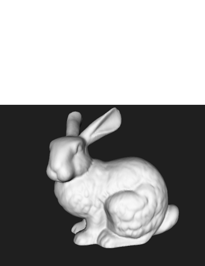
(a) bunny

(b) dragon

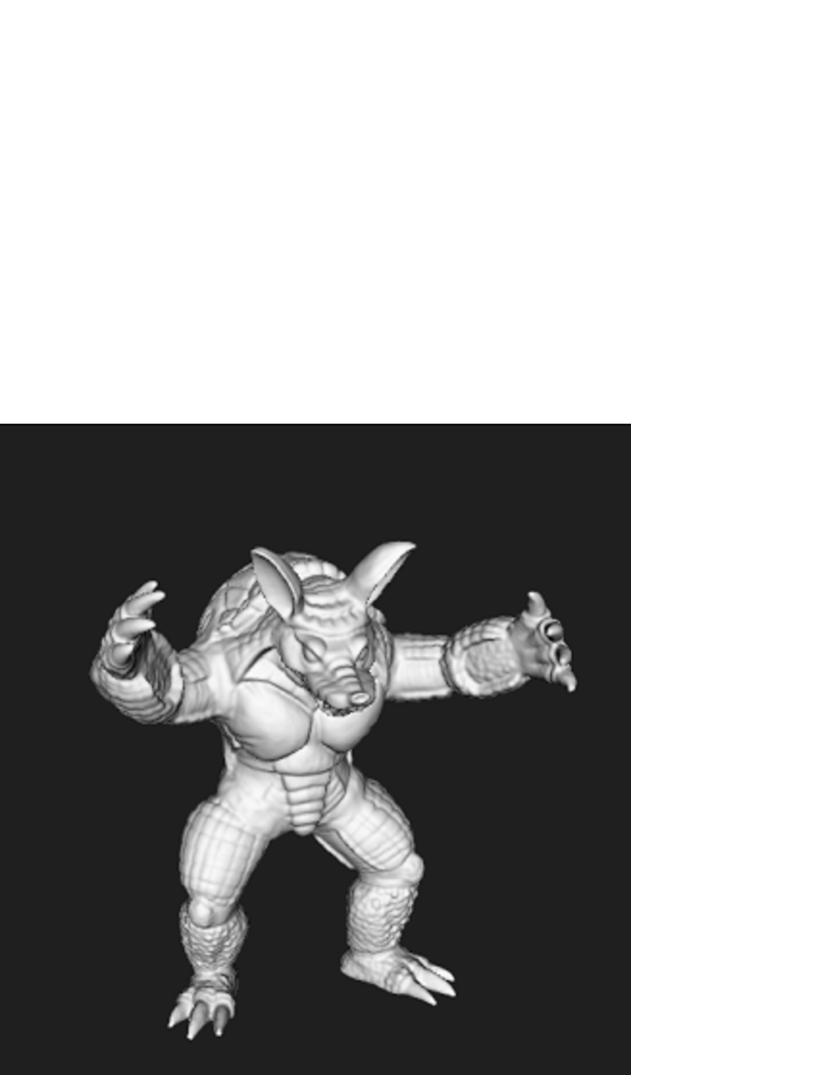
(c) armadillo

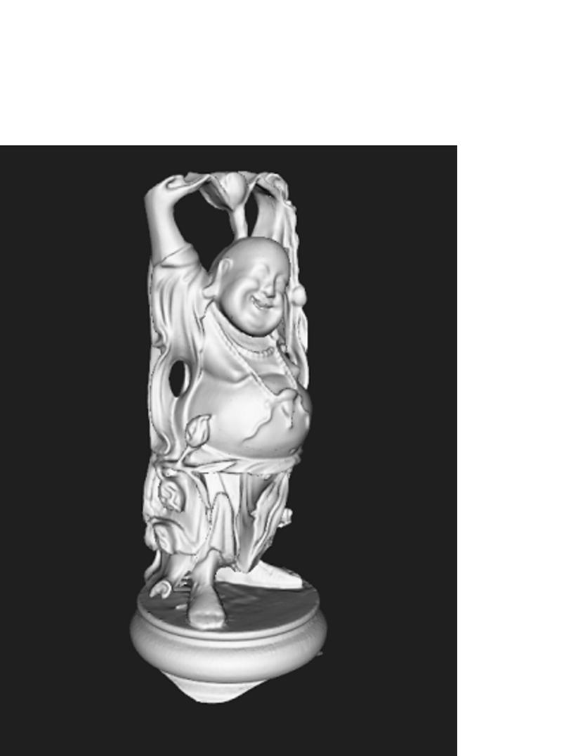
(d) buddha

(e) lucy

Figure 1: Stanford data

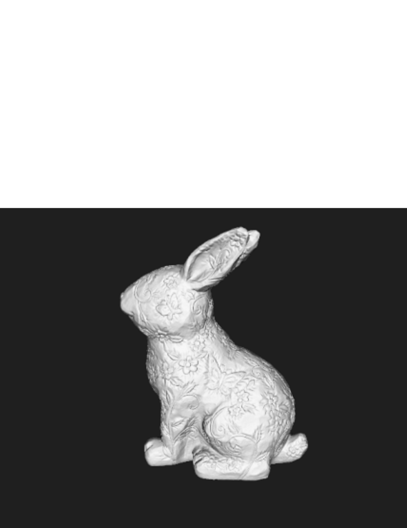
(a) lab bunny

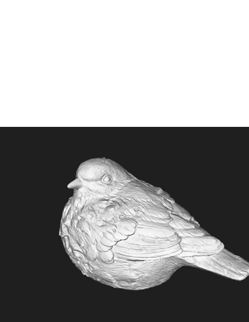
(b) bird

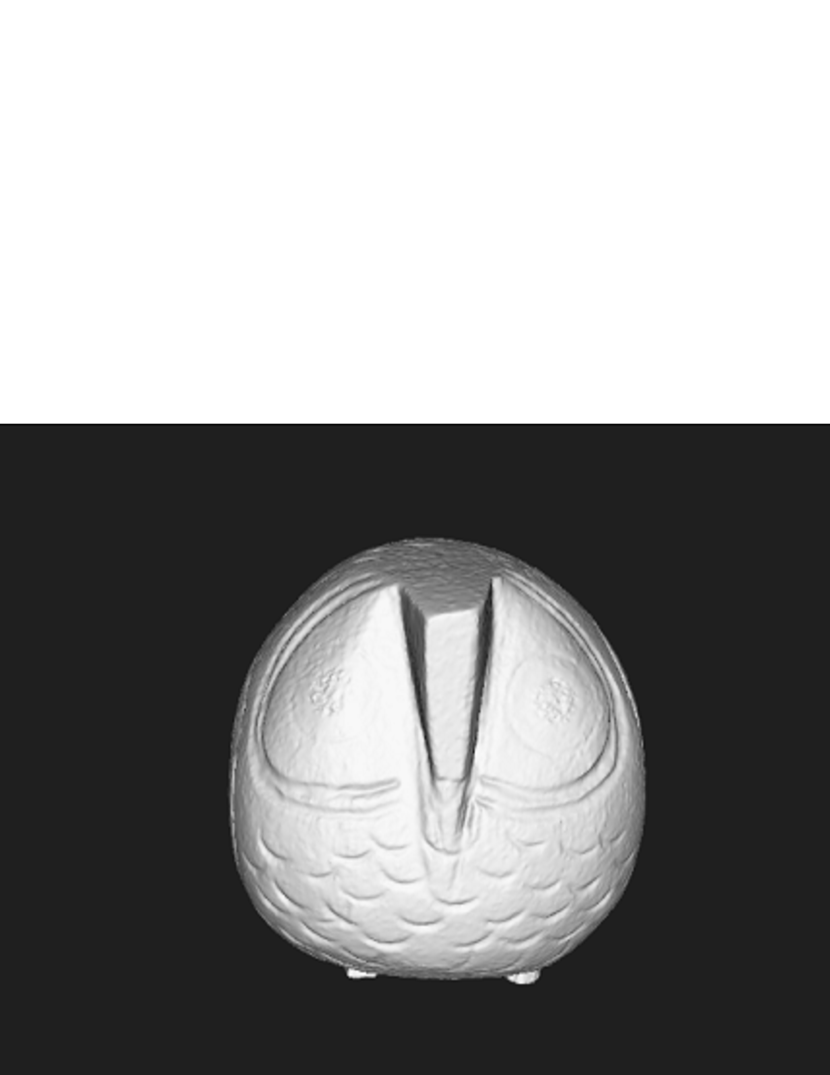
(c) owl

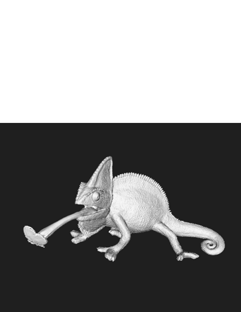
(d) chameleon

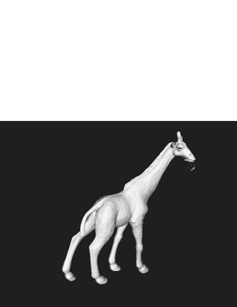
(e) giraffe

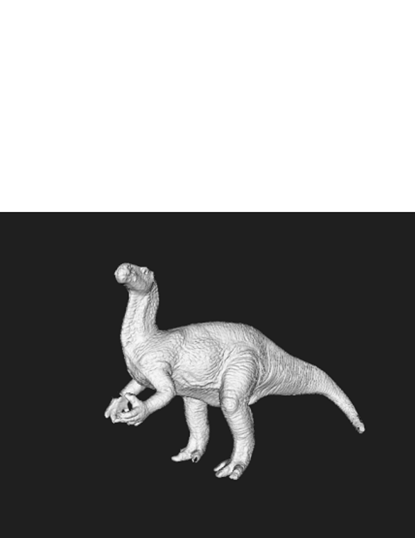
(f) dinosaur

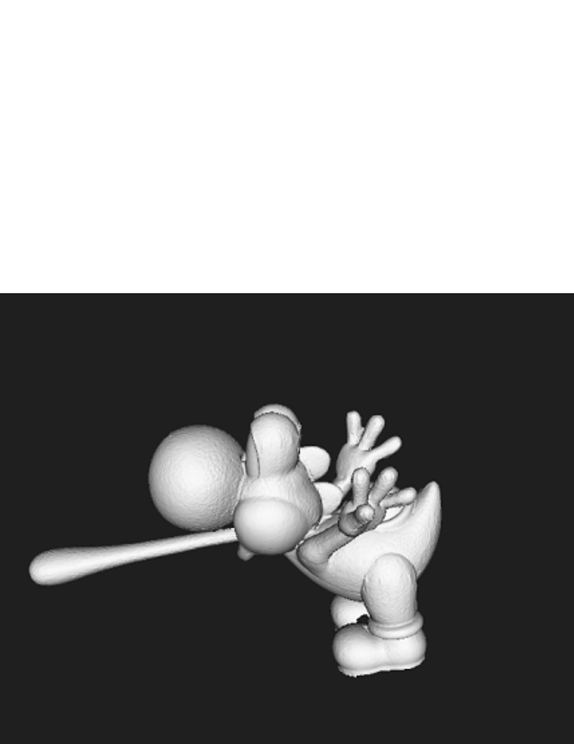
(g) Yoshi

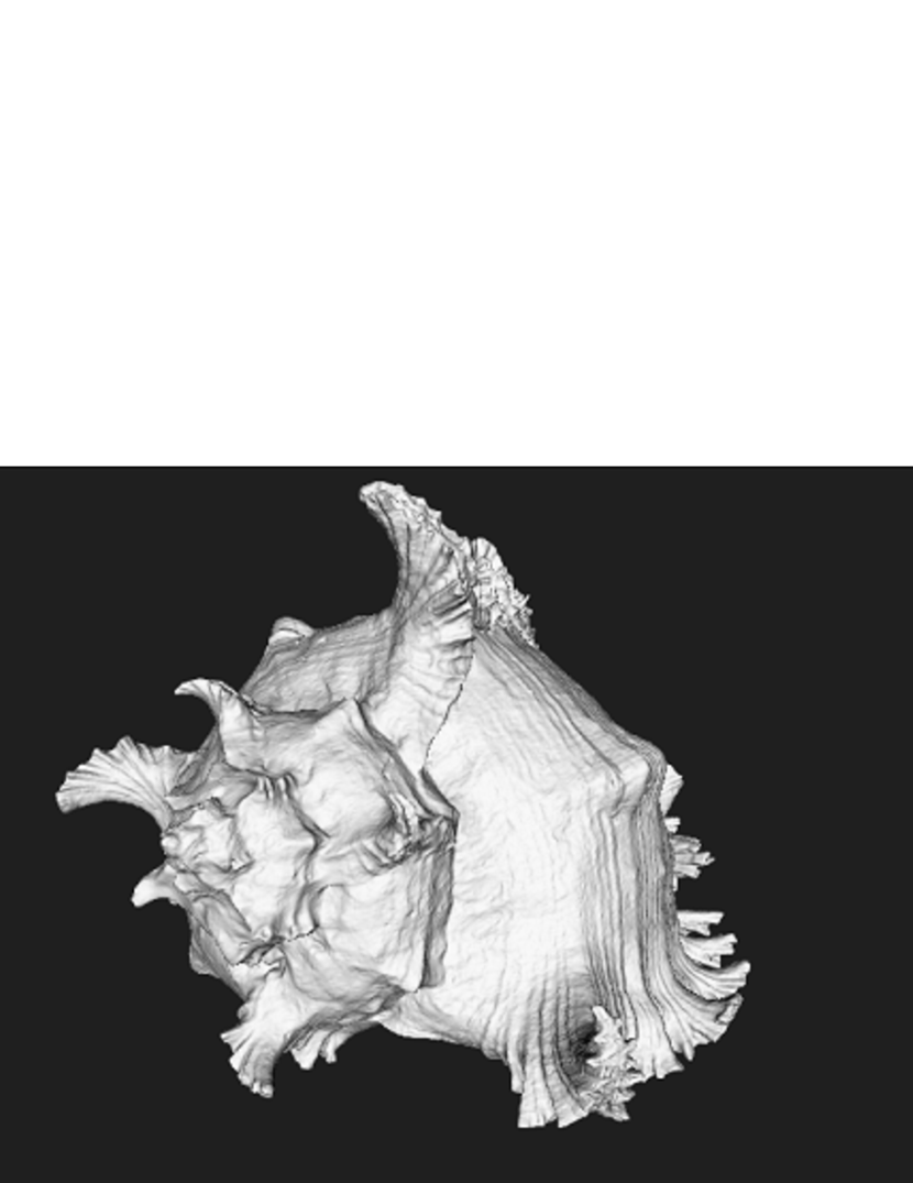
(h) shell

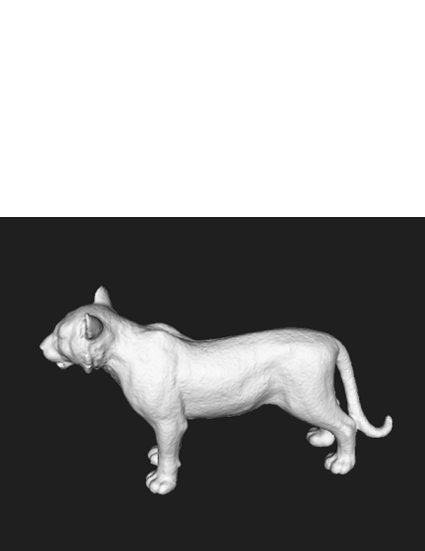
(i) tiger

Figure 2: Laboratory data

4.5 Way of evaluation

In this experiment, Root Mean Square Error (RMSE) is used as the evaluation method on accuracy. Since the ground truth of the rigid transformation is known for the data used in this experiment, the evaluation value is calculated by the following equation using the error between the estimated value and the ground truth.

$$E_{\rm RMSE}= \sqrt{\frac{E^{2}_{X}+E^{2}_{Y}}{|X|+|Y|}}$$ (11)

$$E^{2}_{X}=\sum_{{\bf x}\in X}\left\|\tilde{\mathcal{T}}^{-1}{\bf x}-{\bf x}\right\|^{2}$$

$$E^{2}_{Y}=\sum_{{\bf y}\in Y}\left\|\tilde{\mathcal{T}}{\bf y}-{\bf y}\right\|^{2}$$

Where the two point clouds used for registration are $X,~{}Y$ $\subset\{(x~{}y~{}z~{}1)^{\rm T}$ $|~{}x,~{}y,~{}z\in\mathbb{R}\}$, and the error matrix is $\tilde{\mathcal{T}}=\mathcal{T}_{\rm gt}^{-1}\mathcal{T}$ when the estimated value of the rigid transformation matrix is $\mathcal{T}$ and the ground truth is $\mathcal{T}_{\rm gt}$.

4.6 Experimental result

When we conducted experiments on our method and the comparatives, the overall RMSE results became fig. 3. The RMSE results for Stanford’s data were fig. 4, and the ones for laboratory data were fig. 5. The results show that our method was the most accurate and stable for both data. Also, in the comparative methods, the accuracy of the maximum value was worse in the laboratory data than in the Stanford data. On the other hand, it can be seen that our method maintained accuracy.

The results of actual runtimes of our method and the comparative methods were fig. 6. From the results, we were able to obtain the second highest speed after FGR in terms of median and mean values.

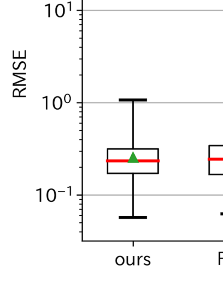
Figure 3: RMSE result of experiments (All Data)

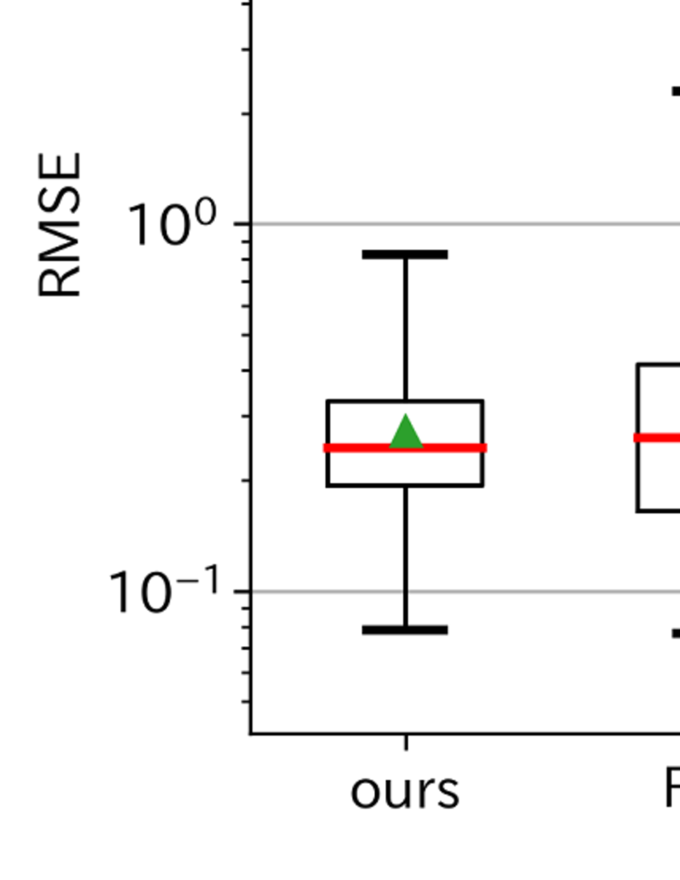
Figure 4: RMSE result of experiments (Stanford Data)

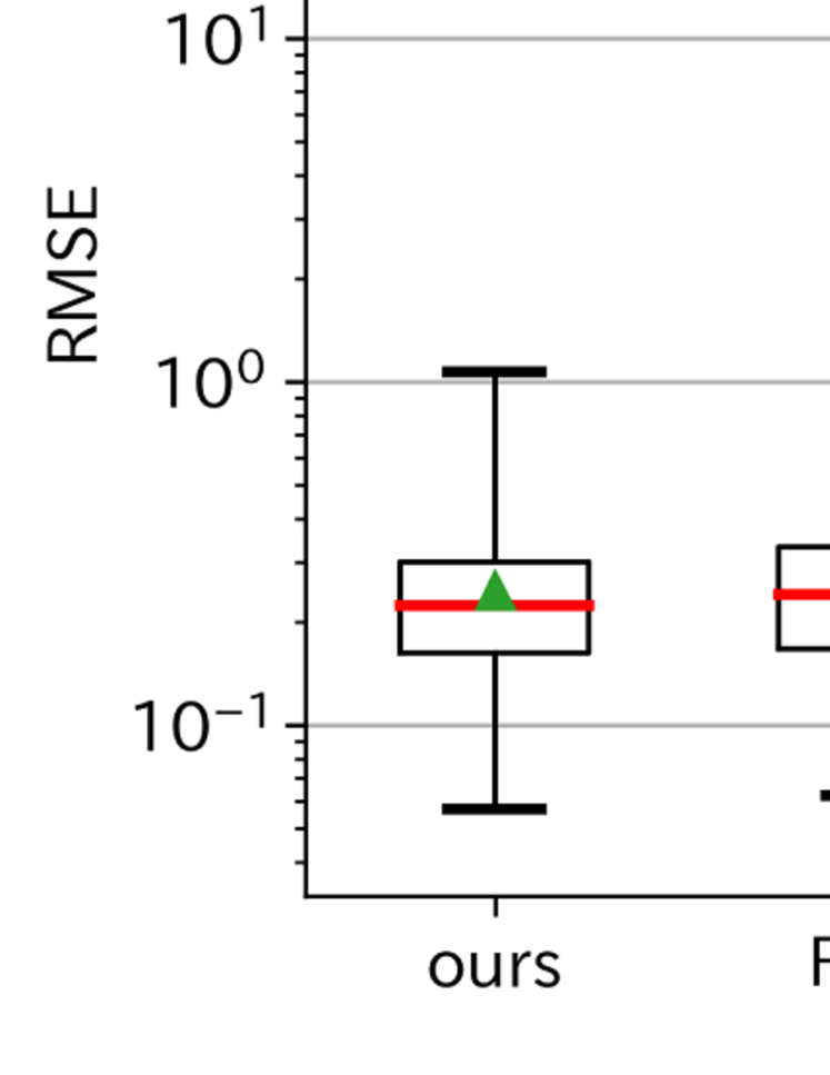
Figure 5: RMSE result of experiments (Lab. Data)

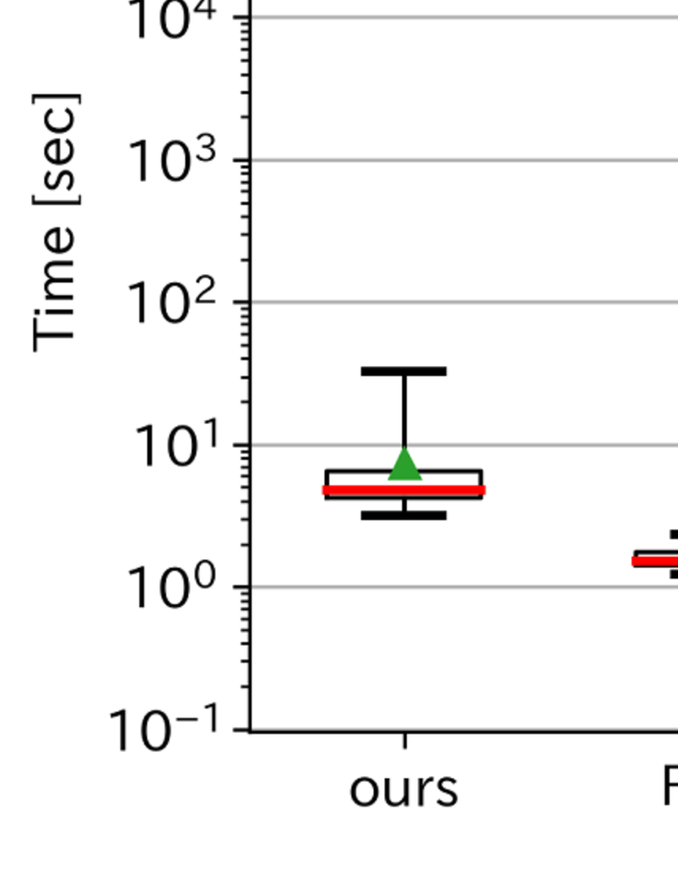
Figure 6: Time result of experiments

We consider why our method obtained stable results with high accuracy. First, if the methods worked well, the accuracy of proposed method did not change significantly from FGR and CPD. This can be seen from the fact that the medians of fig. 3 are close to each other. However, with FGR and CPD, there were cases where some registrations failed. This led to a great lack of stability. Stanford’s Buddha data was the worst, and was significantly inferior to our method in all registrations. The accuracy of the other data often deteriorated at specific registrations.

The reason for this is that CPD uses all points of point clouds and FGR chooses correspondence, but there is a problem in how to choose. Similar to our method, in FGR, the correspondences are selected using the FPFH descriptors and constrained by forming triplets. However, unlike our method, the search of correspondences is performed for all points and this search is stopped when the necessary number has been collected. Therefore, in some results, FGR selected inappropriate points and did not selected good ones. On the other hand, our method excluded inappropriate points by determining the keypoints in advance. As a result, it is considered that our method was very stable compared to the comparative methods.

In addition, our method could be calculated at the speed next to FGR. Considering this reason, first, by using keypoints, our method reduces the point cloud. This made it possible to reduce the number of simple evaluations in subsequent calculations. In addition, although the calculation of triplets is inherently expensive, the appropriate one-to-one correspondences are preferentially used by the preliminary evaluation, and the calculation of triplets is stopped in the middle. Furthermore, since our method does not perform iterative calculation such as continuing the evaluation until the result becomes stable, the calculation time does not increase due to the unstable result. As a result, sufficient speed could be obtained. However, we also found that the calculation of triplets was still expensive, and the algorithm procedure was complicated compared to FGR, so it was not as fast as FGR.

5 Conclusion

In this paper, we proposed a global registration method between 3-dimensional point clouds with high accuracy and stability at a practical speed.

In our method, first the keypoints were extracted from the point cloud, and the one-to-one correspondences were generated using the FPFH descriptors. Furthermore, after obtaining the search priority, we generated triplets using PPF descriptors. The parameters of the rigid transformation were calculated from each triplet, and the rotation vector and translation vector were obtained. Then, histograms were generated for these rotation and translation vectors, and the mode was defined as the rigid transformation between the point clouds.

In the experiment, partial point clouds created from the data of Stanford and the laboratory were used. When compared with other methods such as Fast Global Registration (FGR), our method was sufficiently accurate and had no major failures. As a result, our method obtained high accurate and the most stable results. We think that the reason for this is the selection of keypoints. FGR may select all points. Therefore, for some registrations, FGR selected points where the accuracy of the descriptor was unstable. Other comparative methods likewise failed registration because they used improper points for matching. On the other hand, our method excluded inappropriate points by determining the keypoints in advance. As a result, it is considered that our method was very stable compared to the comparative methods.

In addition, we obtained the result that the calculation speed was second only to FGR by using keypoints and evaluating the priorities of the one-to-one correspondences before the calculation of triplets. Although not as fast as FGR, our method was fast enough given the complexity of the algorithm.

References

- [1] P. Besl and N. D. McKay. “A Method for Registration of 3-D Shapes”. IEEE Transactions on Pattern Analysis and Machine Intelligence(T-PAMI), Vol. 14, No. 2, pp. 239–256, 1992.
- [2] Y. Chen and G. Medioni. “Object Modeling by Registration of Multiple Range Images”. IEEE International Conference Robotics and Automation, Vol. 3, pp. 2724–2729, 1991.
- [3] A. E. Johnson and B. K. Sing. “Registration and integration of textured 3D data”. Image and Vision Computing, Vol. 17, No. 2, pp. 135–147, 1999.
- [4] G. C. Sharp, S. W. Lee and D. K. Wehe. “ICP Registration using Invariant Features”. University of Michigan, Sogang University, 2000.
- [5] S. Granger and X. Pennec. “Multi-scale EM-ICP: A fast and robust approach for surface registration”. European Conference on Computer Vision (ECCV), pp. 418–432, 2002.
- [6] A. Fitzgibbon. “Robust registration of 2D and 3D point sets”. Image and Vision Computing, Vol. 21, No. 13, pp. 1145–1153, 2003.
- [7] J. Yang, H. Li and Y. Jia. “Go-ICP: Solving 3D registration efficiently and globally optimally”. International Conference on Computer Vision (ICCV), pp. 1457–1464, 2013.
- [8] J. Yang, H. Li, D. Campbell and Y. Jia. “Go-ICP: A Globally Optimal Solution to 3D ICP Point-Set Registration”. IEEE Transactions on Pattern Analysis and Machine Intelligence(T-PAMI), Vol. 38, pp. 2241–2254, 2016.
- [9] B. Jian and B. C. Vemuri. “A Robust Algorithm for Point Set Registration Using Mixture of Gaussians”. International Conference on Computer Vision (ICCV), Vol. 2, pp. 1246–1251, 2005.
- [10] H. Chui and A. Rangarajan. “A feature registration framework using mixture models”. IEEE Workshop on Mathematical Methods in Biomedical Image Analysis, pp. 190–197, 2000.
- [11] A. Myronenko and X. Song. “Point Set Registration: Coherent Point Drift”. IEEE Transactions on Pattern Analysis and Machine Intelligence(T-PAMI), Vol. 32, No. 12, pp. 2262–2275, 2010.
- [12] D. Campbell and L. Petersson. “An Adaptive Data Representation for Robust Point-Set Registration and Merging”. International Conference on Computer Vision (ICCV), 2015.
- [13] C. Pu, N. Li and R. B. Fisher. “Robust Rigid Point Registration based on Convolution of Adaptive Gaussian Mixture Models”. Cornell University Library, 2017.
- [14] D. Aiger, N. J. Mitra, and D. Cohen-Or. “4pointss Congruent Sets for Robust Pairwise Surface Registration”. ACM Trans. Graph., Vol. 27, No. 3, pp. 85:1–85:10, August 2008.
- [15] Q.-Y. Zhou, J. Park, and V. Koltun. “Fast Global Registration”. In European Conference on Computer Vision, 2016.
- [16] J. Vongkulbhisal, F. D. l. Torre, and J. P. Costeira. “Discriminative Optimization: Theory and Applications to Computer Vision Problems”. The IEEE Conference on Computer Vision and Pattern Recognition (CVPR), 2017.
- [17] N. Mellado and D. Mitra, Niloy J.and Aiger. “Super 4PCS Fast Global Pointcloud Registration via Smart Indexing”. Computer Graphics Forum, Vol. 33, No. 5, pp. 205–215, 2014.
- [18] J. Vongkulbhisal, B. Irastorza Ugalde, F. D. l. Torre, and J. P. Costeira. “Inverse Composition Discriminative Optimization for Point Cloud Registration”. The IEEE Conference on Computer Vision and Pattern Recognition (CVPR), pp. 2993–3001, 2018.
- [19] R. B. Rusu, N. Blodow, and M. Beetz. “Fast Point Feature Histograms (FPFH) for 3D Registration”. In Proceedings of the 2009 IEEE International Conference on Robotics and Automation, ICRA’09, pp. 1848–1853, Piscataway, NJ, USA, 2009. IEEE Press.
- [20] R. B. Rusu, A. Holzbach, N. Blodow, and M. Beetz. “Fast Geometric Point Labeling Using Conditional Random Fields”. In Proceedings of the 2009 IEEE/RSJ International Conference on Intelligent Robots and Systems, IROS’09, pp. 7–12, Piscataway, NJ, USA, 2009. IEEE Press.
- [21] B. Drost, M. Ulrich, N. Navab, and S. Ilic. “Model globally, match locally: Efficient and robust 3D object recognition”. In 2010 IEEE Computer Society Conference on Computer Vision and Pattern Recognition, pp. 998–1005, June 2010.
- [22] S. Ueyama. “Least-Square Estimation of Transformation Parameters Between Two Point Patterns”. IEEE Transactions on Pattern Analysis and Machine Intelligence(T-PAMI), Vol. 13, No. 4, pp. 376–380, 1991.
- [23] D. Freedman and P. Diaconis. “On the histogram as a density estimator:L2 theory”. Zeitschrift für Wahrscheinlichkeitstheorie und Verwandte Gebiete, Vol. 57, No. 4, pp. 453–476, Dec 1981.
- [24] R. B. Rusu. Semantic 3D Object Maps for Everyday Robot Manipulation. Springer Publishing Company, Incorporated, 2013.
- [25] “The Stanford 3D Scanning Repository”. http://graphics.stanford.edu/data/3Dscanrep/.