Certifying zeros of polynomial systems using interval arithmetic

Abstract

We establish interval arithmetic as a practical tool for certification in numerical algebraic geometry. Our software HomotopyContinuation.jl now has a built-in function certify, which proves the correctness of an isolated nonsingular solution to a square system of polynomial equations. The implementation rests on Krawczyk’s method. We demonstrate that it dramatically outperforms earlier approaches to certification. We see this contribution as powerful new tool in numerical algebraic geometry, that can make certification the default and not just an option.

1 Introduction

Systems of polynomial equations appear in many areas of mathematics, as well as in many applications in the sciences and engineering. In physics and chemistry the geometry of molecules is often modelled with algebraic constraints on the distance or the angle between atoms. In kinematics the relation between robot joints is defined by polynomial equations. In systems biology the steady-state equations for many bio-chemical reaction networks are algebraic equations. A central task in all those applications is computing the isolated zeros of a system of polynomials.

The study of zeros of polynomial systems is at the heart of algebraic geometry. The field of computational algebraic geometry is often associated with symbolic computations based on Gröbner bases. But over the last thirty years numerical algebraic geometry (NAG) [SW05] emerged as an alternative; enabling us to solve problems infeasible with symbolic methods. The algorithmic framework in NAG is numerical homotopy continuation. Several implementations of this are available: Bertini [BHSW], Hom4PS-3 [CLL14], HomotopyContinuation.jl [BT18], NAG4M2 [Ley11] and PHCpack [Ver99]. The first and the third author are the developers of HomotopyContinuation.jl.

Hauenstein and Sottile remark in [HS12] that while all of these softwares “routinely and reliably solve systems of polynomial equations with dozens of variables having thousands of solutions”, they have the shortcoming that “the output is not certified” and that “this restricts their use in some applications, including those in pure mathematics”. To remedy this, Hauenstein and Sottile developed the software alphaCertified [HS12]. It can rigorously certify that Newton’s method, starting at a given numerical approximation, converges quadratically to a true zero by using Smale’s $\alpha$-theory [Sma86]. Hauenstein and Sottile’s contribution to numerical algebraic geometry was a milestone. Yet, alphaCertified produces rigorous certificates using expensive rational arithmetic. This turns the big advantage of numerical computations, namely that they are fast, upside-down and makes certification of large problems prohibitively expensive. Thus, up to this point, the majority of researchers in applied algebraic geometry were kept from using numerical methods, because certification was too expensive and because without certification numerical methods can’t be used for proofs.

We give researchers a new powerful tool in numerical algebraic geometry. Our implementation is integrated in HomotopyContinuation.jl [BT18], so that in principle we can certify all zeros of a system of polynomial equations (see Section 1.2 below for more details). With a fast implementation certification becomes the default and is not just an option and enables the extensive use of numerical methods for rigorous proofs. This is underlined by at least 15 research works [BRST22, BFS21, KPR⁺21, BPS21, BHIM22, Ear21, Mar21, Wei21, LAR21, Stu21, BT21, ABF⁺21, BKK20, SY21, ST21] that have used our implementation in the last two years.

1.1 Contribution

Our contribution to the field of computational and applied algebraic geometry is an extremely fast and easy-to-use implementation of a certification method. This implementation outperforms alphaCertified by several orders of magnitude. It makes the certification of solutions often a matter of seconds and not hours or days. This leap in performance can turn certification in numerical algebraic into default and not just an option.

Starting from version 2.1 HomotopyContinuation.jl has a function certify. The function certify takes as input a square polynomial system $F$ and a numerical approximation of a complex zero $x\in\mathbb{C}^{n}$ (or a list of zeros). If the output says “certified”, then this is a rigorous proof that a solution of $F=0$ is near $x$. If the output says “not certified”, then this does not necessarily mean that there is no zero near $x$, just that the method couldn’t find one. Figure 2 shows an example of certify.

We combine interval arithmetic and Krawczyk’s method with numerical algebraic geometry to rigorously certify solutions to square systems of polynomial equations. In technical terms, our implementation returns strong interval approximate zeros. We introduce this notion in Definition 3.7 below. The strong interval approximate zero consists of a box in $\mathbb{C}^{n}$, which contains a unique true zero of the polynomial system. If the input is a list of zeros, the routine returns a list of distinct strong interval approximate zeros. Therefore, our method can be used to prove hard lower bounds on the number of zeros of a polynomial system. Combined with theoretical upper bounds this can constitute rigorous mathematical proofs on the number of zeros of such systems. We explain this in more detail in the next subsection. In addition, if the given polynomial system is real, we give a certificate whether the certified zero is a real zero (the approximate zero does not need to be real for this). The returned boxes may also be used to verify if a real zero is positive real. Therefore, our method can also be used to prove lower bounds on the number of real and positive real zeros of a polynomial system.

It is also possible to give a square system of rational functions as input to our implementation. Although this article is mostly formulated in terms of polynomial systems, Krawczyk’s method also applies to square systems of rational functions (in fact, to all analytic functions $\mathbb{R}^{n}\to\mathbb{R}^{n}$; see Section 3). Consequently, all statements about using our implementation for proofs are equally valid of square systems of rational functions.

1.2 Certifying all zeros

Our implementation is integrated in HomotopyContinuation.jl [BT18]. This is a software for numerically solving systems of polynomials equations via homotopy continuation. The basic idea is as follows: suppose that $F(x)=(f_{1}(x),\ldots,f_{n}(x))$ is a system of polynomials in $n$ variables $x=(x_{1},\ldots,x_{n})$. To compute the solutions of the systems of equation $F(x)=0$ one takes another system of polynomials $G(x)=(g_{1}(x),\ldots,g_{n}(x))$, called start system, for which the zeros are simple to compute. Then, $F$ and $G$ are joined with a path in the vector space of systems of polynomials. This path defines a homotopy $H(x,t):\mathbb{C}^{n}\times\mathbb{C}\to\mathbb{C}$, such that $H(x,1)=G(x)$ and $H(x,0)=F(x)$. The zeros of $G$ are continued towards the zeros of $F$ by solving the ODE initial value problems $\tfrac{\partial H}{\partial t}+\tfrac{\partial H}{\partial x}\dot{x}(t)=0$, where $x(1)$ ranges over the zeros of $G$. For more details see the textbook [SW05].

In the last paragraph there is nothing special about polynomials. This approach works for any analytic functions $F$ and $G$. However, in the case of systems of polynomial equations we can choose $G$ such that we compute all zeros of $F$. This follows from the Parameter Continuation Theorem by Morgan and Sommese [MS89]: suppose that $F(x)=F(x;p_{0})$ is a point in family of polynomials systems $F(x;p)$ that depends polynomially on parameters $p\in\mathbb{C}^{k}$. The Parameter Continuation Theorem says that there exists a proper algebraic subvariety $\Sigma\subset\mathbb{C}^{k}$ with the following property. Let $\gamma(t)\colon[0,1]\rightarrow\mathbb{C}^{k}$ with $\gamma(0)=p_{0}$ be a continuous path and $H(x,t)$ the corresponding homotopy. If $\gamma((0,1])\cap\Sigma=\emptyset$, then as $t\to 0$, the limits of the solution paths $x(t)$ with $H(x(t),t)=0$ include all the isolated solutions to $F(x;p_{0})=0$. This includes both regular solutions and solutions with multiplicity greater than one. Consequently, every parameter outside $\Sigma$ provides a suitable start system for $F$.

The Parameter Continuation Theorem implies the existence of start systems, such that we can compute all zeros of $F$, but it does not tell us how to set up these start systems, nor how to compute their zeros. In fact, different choices of families of parametrized systems lead to different start systems and thus different homotopy methods. In HomotopyContinuation.jl [BT18] one can choose between two well-established strategies for choosing start systems: the so-called totaldegree start system and the polyhedral start system [HS95].

Coming back to interval arithmetic we see that the zeros computed by polynomial homotopy continuation can be used as input for certification, so that we can certify all solutions of a system of polynomial equations. There is one subtlety, though. Although the Parameter Continuation Theorem asserts that in principle we can find all solutions, since homotopy continuation involves numerical computations we can’t rule out the possibiliy that some computations of solutions paths fail. Still, combining certification with homotopy continuation always gives lower bounds on the number of zeros. This can be exploited in situations, where we know upper bounds. An example of such a scenario in enumerative geometry is discussed in Section 5.1 below, where we certify 3264 real zeros of a system of polynomials that is known to have at most 3264 complex zeros. Another example from optimization is discussed in [BSW21, Section 3.3]. Here, certifying all zeros of a system of polynomial equations helps to rigorously compute the minimal Euclidean distance of a point to an algebraic hypersurface.

1.3 Comparison to previous works

There are other implementations of certification methods using Krawczyk’s method and interval arithmetic, e.g., the commercial MATLAB package INTLAB [Rum99], the Macaulay2 package NumericalCertification [Lee19], and the Julia package IntervalRootFinding.jl [BS]. The theory of Krawczyk’s method and interval arithmetic are explained, for instance, in [Rum83].

Compared to INTLAB, the source code of our implementation is freely available and can be verified by anyone. Additionally, INTLAB doesn’t support the use of arbitrary precision interval arithmetic which limits its capability to certify badly conditioned solutions. NumericalCertification, as of version 1.0, takes as input not the numerical approximation of a complex zero $x\in\mathbb{C}^{n}$, but instead a box $I$ in $\mathbb{C}^{n}$. Then, NumericalCertification attempts to certify that interval $I$ is a strong interval approximate. The process of going from a numerical approximation $x$ to a good candidate interval $I$ needs particular care, as illustrated in Section 4. INTLAB and NumericalCertification also both require manual work to obtain a list of all distinct distinct strong interval approximate zeros. The package IntervalRootFinding.jl can find all zeros of a multivariate function inside a given box in $\mathbb{R}^{n}$, whereas our implementation works in $\mathbb{C}^{n}$ and additionally certifies reality of zeros; see Section 7.

1.4 Acknowledgements

We thank Pierre Lairez for a discussion that initiated this project and for several helpful subsequent discussions on the topic. We thank anonymous referees for useful feedback that improved the article.

1.5 Outline

The rest of this article is organized as follows. In the next two sections we give a short introduction to interval arithmetic and explain the Krawczyk method. Section 4 focuses on implementation details. In Section 5 we demonstrate features of our implementations using two examples. For completeness, we give a proof of Krawczyk’s method in Section 6, and in Section 7 we discuss how to certify reality of zeros.

2 Interval arithmetic

Before we discuss our implementation, let us briefly introduce the basics of interval arithmetic.

Since the 1950s researchers [Moo66, Sun58] have worked on interval arithmetic, which allows certified computations while still using floating point arithmetic. We briefly introduce the concepts from interval arithmetic which are relevant for our article.

2.1 Real interval arithmetic

Real interval arithmetic concerns computing with compact real intervals. Following [May17] we denote the set of all compact real intervals by

$$\mathbb{I}\mathbb{R}:=\{[a,b]\mid a,b\in\mathbb{R},a\leq b\}.$$

For $X,Y\in\mathbb{IR}$ and the binary operation $\circ\in\{+,-,\cdot,/\}$ we define

$$X\circ Y=\{x\circ y\,|\,x\in X,y\in Y\},$$ (1)

where we assume $0\notin Y$ in the case of division. The interval arithmetic version of these binary operations, as well as other standard arithmetic operations, have explicit formulas. See, e.g., [May17, Sec. 2.6] for more details.

2.2 Complex interval arithmetic

We define the set of rectangular complex intervals as

$$\mathbb{IC}:=\{X+iY\mid X,Y\in\mathbb{IR}\},$$

where $X+iY=\{x+iy\mid x\in X,y\in Y\}$ and $i=\sqrt{-1}$. Following [May17, Ch. 9] we define the algebraic operations for $I=X+iY,J=W+iZ\in\mathbb{IC}$ in terms of operations on the real intervals from (1):

$$I+J :=(X+W)+i(Y+Z),\qquad I\cdot J :=(X\cdot W-Y\cdot Z)+i(X\cdot Z+Y\cdot W)$$ (2)

$$I-J :=(X-W)+i(Y-Z),\qquad\;\,\frac{I}{J} :=\frac{X\cdot W+Y\cdot Z}{W\cdot W+Z\cdot Z}+i\frac{Y\cdot W-X\cdot Z}{W\cdot W+Z\cdot Z}.$$

It is necessary to use (1) instead of complex arithmetic for the definition of algebraic operations in $\mathbb{IC}$. The following example from [May17] demonstrates this. Consider the intervals $I=[1,2]+i[0,0]$ and $J=[1,1]+i[1,1]$. Then, $\{x\cdot y|x\in I,y\in J\}=\{t(1+i)\mid 1\leq t\leq 2\}$ is not a rectangular complex interval, while $I\cdot J=[1,2]+i[1,2]$ is.

The algebraic structure of $\mathbb{IC}$ is given by following theorem; see, e.g., [May17, Theorem 9.1.4].

Theorem 2.1.

The following holds.

1. $(\mathbb{IC},+)$ is a commutative semigroup with neutral element.

2. $(\mathbb{IC},+,\cdot)$ has no zero divisors.

Furthermore, if $I,J,K,L\in\mathbb{IC}$, then

1. $I\cdot(J+K)\subseteq I\cdot J+I\cdot K$, but equality does not hold in general.

2. $I\subseteq J,K\subseteq L$, then $I\circ K\subseteq J\circ L$ for $\circ\in\{+,-,\cdot,/\}$.

Working with interval arithmetic is challenging because of the third item from the previous theorem: distributivity does not hold in $\mathbb{IC}$. As a consequence, in $\mathbb{IC}$ the evaluation of polynomials depends on the exact order of the evaluation steps. Therefore, the evaluation of polynomial maps $F:\mathbb{IC}^{n}\to\mathbb{IC}$ is only well-defined if $F$ is defined by a straight-line program, and not just by a list of coefficients. Figure 1 demonstrates this issue in an example. See, e.g., [BCS13, Sec. 4.1] for an introduction to straight-line programs.

Figure 1: The picture shows two straight-line programs for evaluating the polynomial $f(x,y,z)=(x+y)z$. Let $I=([-1,0],\,[1,1],\,[0,1])^{T}$. Then, the program on the left evaluated at $I$ yields $f(I)=([-1,0]+[1,1])[0,1]=[0,1]$, while the program on the right yields $f(I)=[-1,0][0,1]+[1,1][0,1]=[-1,1]$.

Arithmetic in $\mathbb{IC}^{n}$ is defined in the expected way. If $I=(I_{1},\ldots,I_{n}),J=(J_{1},\ldots,J_{n})\in\mathbb{IC}^{n}$,

$$I+J=(I_{1}+J_{1},\ldots,I_{n}+J_{n}).$$

Scalar multiplication for $I\in\mathbb{IC}$ and $J\in\mathbb{IC}^{n}$ is defined as $I\cdot J=(I\cdot J_{1},\ldots,I\cdot J_{n})$. The product of an interval matrix $A=(A_{i,j})\in\mathbb{IC}^{n\times n}$ and an interval vector $I\in\mathbb{IC}^{n}$ is

$$A\cdot I:=I_{1}\cdot\begin{bmatrix}A_{1,1}\\ \vdots\\ A_{n,1}\end{bmatrix}+\cdots+I_{n}\cdot\begin{bmatrix}A_{1,n}\\ \vdots\\ A_{n,n}\end{bmatrix}.$$ (3)

Similar to the one-dimensional case $(\mathbb{IC}^{n},+)$ is a commutative semigroup with neutral element.

3 Certifying zeros with interval arithmetic

In 1969 Krawczyk [Kra69] developed an interval arithmetic version of Newton’s method. Later in 1977 Moore [Moo77] recognized that Krawczyk’s method can be used to certify the existence and uniqueness of a solution to a system of nonlinear equations. Interval arithmetic and interval Newton’s method are a prominent tool in many areas of applied mathematics; e.g., in chemical engineering [GS05], thermodynamics [GD05] and robotics [KSS15]. See also the overview in [Rum10].

The results in this section are stated for general functions. For a practical implementation it is however necessary to compute interval enclosures (see Definition 3.1). We discuss our approach in the context of polynomial systems in Section 4.1 below. A generalization in this spirit is discussed in [BLL19].

3.1 Krawczyk’s method

In this section we recall Krawczyk’s method. First, we need three definitions.

Definition 3.1 (Interval enclosure).

Let $F:\mathbb{C}^{n}\rightarrow\mathbb{C}^{n}$. A map $\square F:\mathbb{IC}^{n}\rightarrow\mathbb{IC}^{n}$ is an interval enclosure of $F$ if for every $I\in\mathbb{IC}^{n}$ we have $\{F(x)\mid x\in I\}\subseteq\square F(I).$

In the rest of this article we use the notation $\square F$ to denote the interval enclosure of $F$. Also, we do not distinguish between a point $x\in\mathbb{C}^{n}$ and the complex interval $[\mathrm{Re}(x),\mathrm{Re}(x)]+i[\mathrm{Im}(x),\mathrm{Im}(x)]$ defined by $x$. We simply use the symbol “$x$” for both terms so that $\square F(x)$ is well-defined.

Definition 3.2 (Interval matrix norm).

Let $A\in\mathbb{IC}^{n\times n}$. We define the operator norm of $A$ as $\|A\|_{\infty}:=\max\limits_{B\in A}\max\limits_{v\in\mathbb{C}^{n}}\tfrac{\|Bv\|_{\infty}}{\|v\|_{\infty}},$ where $\|(v_{1},\ldots,v_{n})\|_{\infty}=\max_{1\leq i\leq n}|v_{i}|$ is the infinity norm in $\mathbb{C}^{n}$.

Next we introduce an interval version of the Newton operator, the Krawczyk operator [Kra69].

Definition 3.3.

Let $F:\mathbb{C}^{n}\rightarrow\mathbb{C}^{n}$ be differentiable, and $\mathrm{J}F$ be its Jacobian matrix seen as a function $\mathbb{C}^{n}\to\mathbb{C}^{n\times n}$. Let $\square F$ be an interval enclosure of $F$ and $\square\mathrm{J}F$ be an interval enclosure of $\mathrm{J}F$. Furthermore, let $I\in\mathbb{IC}^{n}$ and $x\in\mathbb{C}^{n}$ and let $Y\in\mathbb{C}^{n\times n}$ be an invertible matrix. We define the Krawczyk operator

$$K_{x,Y}(I):=x-Y\cdot\square F(x)+(\mathbf{1}_{n}-Y\cdot\square\mathrm{J}F(I))(I-x).$$

Here, $\mathbf{1}_{n}$ is the ${n\times n}$-identity matrix.

Remark 3.4.

In the literature, $K_{x,Y}(I)$ is often defined using $F(x)$ and not $\square F(x)$. Here, we use this definition, because in practice it is usually not feasible to evaluate $F(x)$ exactly. Instead, $F(x)$ is replaced by an interval enclosure.

Remark 3.5.

The second part of Theorem 3.6 motivates to find a matrix $Y\in\mathbb{C}^{n\times n}$ such that $||1_{n}-Y\cdot\square\mathrm{J}F(I)||_{\infty}$ is minimized. A good choice is an approximation of the inverse of $\mathrm{J}F(x)$.

We are now ready to state the theorem behind Krawczyk’s method. The first proof for real interval arithmetic is due to Moore [Moo77]. A proof for complex data is at least known since the work by Rump [Rum83]. We recall the proof from [BLL19] in Section 6 below. Note that all the data in the theorem can be computed using interval arithmetic.

Theorem 3.6.

Let $F:\mathbb{C}^{n}\rightarrow\mathbb{C}^{n}$ be differentiable and $I\in\mathbb{IC}^{n}$. Let $x\in I$ and $Y\in\mathbb{C}^{n\times n}$ be an invertible complex $n\times n$ matrix. The following holds.

1. If $K_{x,Y}(I)\subset I$, there is a zero of $F$ in $I$.

2. If additionally $\sqrt{2}\,\lVert\mathbf{1}_{n}-Y\square\mathrm{J}F(I)\rVert_{\infty}<1$, then $F$ has exactly one zero in $I$.

To simplify our language when talking about intervals $I\in\mathbb{IC}^{n}$ satisfying Theorem 3.6 we introduce the following definitions.

Definition 3.7.

Let $F:\mathbb{C}^{n}\rightarrow\mathbb{C}^{n}$ be differentiable and $I\in\mathbb{IC}^{n}$. Let $K_{x,Y}(I)$ be the associated Krawczyk operator (see Definition 3.3). If there exists an invertible matrix $Y\in\mathbb{C}^{n\times n}$, such that $K_{x,Y}(I)\subset I$, we say that $I$ is an interval approximate zero $F$. We call $I$ a strong interval approximate zero of $F$ if in addition $\sqrt{2}\lVert\mathbf{1}_{n}-Y\square\mathrm{J}F(I)\rVert_{\infty}<1$ .

Remark 3.8.

The name “strong interval approximate zero” is not common in the field of interval arithmetic. We introduce it as a reference to the work of Shub and Smale and the software alphaCertified [HS12] that inspired our work. Shub and Smale coined the name strong approximate zero for points in the radius of quadratic convergence of Newton’s method.

Definition 3.9.

If $I$ is an interval approximate zero, then, by Theorem 3.6, $I$ contains a zero of $F$. We call such a zero an associated zero of $I$. If $I$ is a strong interval approximate zero then there is a unique associated zero and we refer to is as the associated zero of $I$.

The notion of strong interval approximate zero is stronger than the definition suggests at first sight. We not only certify that a unique zero of $F$ exists inside $I$, but even that we can approximate this zero with arbitrary precision. This is shown in the next proposition, which we prove in Section 6

Proposition 3.10.

Let $I$ be a strong interval approximate zero of $F$ and let $x^{*}\in I$ be the unique zero of $F$ inside $I$. Let $x\in I$ be any point in $I$. We define $x_{0}:=x$ and for all $i\geq 1$ we define the iterates $x_{i}:=x_{i-1}-Y\,F(x_{i-1})$, where $Y\in\mathbb{C}^{n\times n}$ is the matrix from Definition 3.7. Then, the sequence $(x_{i})_{i\geq 0}$ converges (at least linearly) to $x^{*}$.

4 Implementation details

In this section we describe details of our implementation of Krawcyzk’s method.

The certification routine takes as input a square polynomial system $F:\mathbb{C}^{n}\rightarrow\mathbb{C}^{n}$ and a finite list $X\subset\mathbb{C}^{n}$ of (suspected) approximations of isolated nonsingular zeros of $F$. It is also possible to provide a square system of rational functions as input, but in the following we focus in polynomial systems for simplicity. Our implementation returns a list of strong interval approximate zeros $\mathcal{I}=\{I_{1},\ldots,I_{m}\}$ in $\mathbb{IC}^{n}$, such that no two intervals $I_{k}$ and $I_{\ell}$, $k\neq\ell$, overlap. If two strong interval approximate zeros don’t overlap then this implies that their associated zeros are distinct. Additionally, if $F$ is a real polynomial system then for each $I_{k}\in\mathcal{I}$ it is determined whether its associated zero is real. The prototypical application of the certification routine is to take as input approximations of all isolated nonsingular solutions $X\subset\mathbb{C}^{n}$ of $F$ as computed by numerical homotopy continuation methods as discussed in Section 1.2.

4.1 Interval enclosures for polynomial systems

The fact that distributivity doesn’t hold in $\mathbb{IC}$ makes it necessary for us to define the polynomial system $F:\mathbb{C}^{n}\to\mathbb{C}^{n}$, and its interval enclosure $\square F$, by a straight-line program, and not just by a list of coefficients. The overestimation of the interval enclosure $\square F$ increases with the size of the straight line program. Therefore, it is good to express $F$ and its enclosure $\square F$ by the smallest straight line program possible. To achieve this, HomotopyContinuation.jl automatically applies a multivariate version of Horner’s rule to reduce the number of operations necessary to evaluate $F$ and $\square F$.

Remark 4.1.

Our implementation of interval enclosures can also be used to prove that a polynomial map $F:\mathbb{C}^{n}\to\mathbb{C}^{m}$ with real coefficients, evaluated at a real point $p\in\mathbb{R}^{n}$, is positive. To verify this, one takes an interval $I\in\mathbb{IC}^{n}$ of the form $I=J+i[0,0]^{\times n}$ such that $p\in J$. If $\square F$ is an interval enclosure of $F$, and if $\square F(I)\subset\mathbb{R}_{>0}^{m}+i[0,0]^{\times m}$, then this is a proof that $F(p)\in\mathbb{R}_{>0}^{m}$.

4.2 Machine interval arithmetic

In the next subsection we give a method to construct an candidate $I\in\mathbb{IC}^{n}$ for a strong interval approximate zero. Before, we need to study machine interval arithmetic; the realization of interval arithmetic with finite precision floating point arithmetic. We assume the standard model of floating point arithmetic [Hig02, Section 2.3], where the result of a floating point operation is accurate up to relative unit roundoff $u$: $\mathrm{fl}(x\circ y)=(x\circ y)(1+\delta),$ where $|\delta|\leq u$ and $\circ\in\{+,-,*,/\}$. For instance, following the IEE-754 standard, the unit roundoff in double precision arithmetic is $u=2^{-53}\approx 2.2\cdot 10^{-16}$. The key property in the context of interval arithmetic is that each result of a floating point operation can be rounded outwards, such that the resulting interval contains the true (exact) result; see, e.g., [May17, Section 3.2]. Therefore, given $X,Y\in\mathbb{IC}$ the result of $X\circ Y$, $\circ\in\{+,-,*,/\}$, is $\mathrm{fl}(X\circ Y):=\{(x\circ y)(1+\delta)\,|\,|\delta|\leq u,x\in X,y\in Y\}$ in machine arithmetic. This interval contains $X\circ Y$. It is larger. Additionally, for a given $x\in\mathbb{IC}$, all intervals of the form $\{x+(|\mathrm{Re}(x_{j})|+i|\mathrm{Im}(x_{j})|)\delta\,|\,|\delta|\leq\mu\}$ with $0<\mu\leq u$ are indistinguishable when working with precision $u$.

Consequently it is possible that the Krawczyk operator $K_{\tilde{x},Y}$, see Definition 3.3, is a contraction for the interval $I$, but that machine arithmetic can’t verify this, because $\mathrm{fl}(X\circ Y)$ is larger than $X\circ Y$. In such a case, the unit roundoff $u$ needs to be sufficiently decreased. For this reason our implementation uses machine interval arithmetic based on double precision arithmetic as well as, if necessary, the arbitrary precision interval arithmetic implemented in Arb [Joh17]. For instance, we could not certify all solutions in the example in Section 5.1 below using only 64-bit arithmetic, because the zeros are too ill-posed.

4.3 Determining strong interval approximate zeros

In a first step, the certification routine attempts to produce for a given $x\in X$ a strong interval approximate zero $I\in\mathbb{IC}^{n}$. Recall that for $I\in\mathbb{IC}^{n}$ to be a strong interval approximate zero we need by Theorem 3.6 to have a point $\tilde{x}\in I$, and a matrix $Y\in\mathbb{C}^{n\times n}$ such that $K_{\tilde{x},Y}(I)\subset I$, and $\sqrt{2}\,\lVert\mathbf{1}_{n}-Y\square\mathrm{J}F(I)\rVert_{\infty}<1$.

Given a point $x\in X$ and a unit roundoff $u$, the point $x$ is refined using Newton’s method to maximal accuracy. We denote this refined point $\tilde{x}$. Here, we assume that $x$ is already in the region of quadratic convergence of Newton’s method. Next, the point $\tilde{x}$ needs to be inflated to an interval $I$ with $\tilde{x}\in I$. This process is called $\varepsilon$-inflation in the literature [May17, Sec. 4.3]. However, choosing the correct $I$ is a hard problem: if $I$ is too small or too large, then the Krawcyzk operator is not a contraction.

In spite of these difficulties, we found the following heuristic to determine $I$ work very well. First, we compute $JF(\tilde{x})^{-1}$ in floating arithmetic, which yields a matrix $Y$. Then, we set

$$I:=(\tilde{x}_{j}\pm|(Y\cdot\square F(x))_{j}|u^{-\frac{1}{4}})_{j=1,\ldots,n},$$

where $u$ is the unit roundoff. The motivation behind this choice is as follows: If we assume $\tilde{x}$ to be in the region of quadratic convergence of Newton’s method, it follows from the Newton-Kantorovich theorem that $||\mathrm{J}F(\tilde{x})^{-1}F(\tilde{x})||_{\infty}$ is a good estimate of the distance between $\tilde{x}$ and the convergence limit $x^{*}$. This distance is approximated by $(Y\cdot\square F(x))_{j}$ for $1\leq j\leq n$. The factor $u^{-\frac{1}{4}}$ accounts for the overestimation by machine interval arithmetic. Here is how we arrived at this factor: The best relative accuracy we can expect to get for the $j$-th entry of $x^{*}$ is about $|(x^{*})_{j}|\cdot u$, so that $||I-x^{*}||_{\infty}$ needs to be larger than $(|(x^{*})_{j}|u)^{-1/2}$ for quadratic convergence. On the other hand, we need to have an $\varepsilon$-inflation of at least $|(Y\cdot\square F({x}))_{j}|$ so that the inflated interval contains $(x^{*})_{j}$. In the typical case we have $|(Y\cdot\square F({x}))_{j}|>1$, i.e., $|(Y\cdot\square F({x}))_{j}|>|(Y\cdot\square F({x}))_{j}|^{\frac{1}{2}}$. All of this motivates us to use $|(Y\cdot\square F({x}))_{j}|u^{-\frac{1}{2}}$ as the inflation constant. However, to account for hidden constant factors we need to increase this estimate. We found that replacing $u^{-\frac{1}{2}}$ by $u^{-\frac{1}{4}}$ produces a good estimate that works well in all the examples we tested.

Finally, if $I$ doesn’t satisfy the conditions in Theorem 3.6 the procedure is repeated with a smaller unit roundoff $u$. This repeats until either a minimal unit roundoff is reached or the certification is successful.

4.4 Producing distinct intervals

Assume now that the steps in Section 4.3 have been performed for all $x\in X$. We obtain a list of strong interval approximate zeros $I_{1},\ldots,I_{r}\in\mathbb{IC}^{n}$. In a final step we want to select a subset $M\subset\{1,\ldots,r\}$ such that for all $k,j\in M$, $k\neq j$, the intervals $I_{k}$ and $I_{j}$ do not overlap. If two strong interval approximate zeros do not overlap then it is guaranteed that they have distinct associated zeros. A simple approach to determine $M$ is to compare all intervals pairwise. However, this approach requires us to perform ${r\choose 2}$ interval vector comparisons. For larger problems this becomes prohibitively expensive: in the example in Section 5.2 the number of necessary comparisons is already larger than $4\cdot 10^{9}$.

Instead, we employ the following improved scheme to determine all non-overlapping intervals. First, we pick a random point $q\in\mathbb{C}^{n}$ and compute in interval arithmetic for each $I_{k}$, $k\in M$, the squared Euclidean distance $d_{k}\in\mathbb{IR}$ between $I_{k}$ and $q$. Due to the guarantees of interval arithmetic we have that $d_{k}$ and $d_{\ell}$ overlap if $I_{k}$ and $I_{\ell}$ overlap (but the converse it not necessarily true). Next, we check for all overlapping intervals $d_{k},d_{\ell}\in\{d_{k}\in\mathbb{IR}\,|\,k=1,\ldots,r\}$, whether $I_{k}$ and $I_{\ell}$ overlap, and if so, we group them accordingly. This allows us to construct the set $M$ by selecting those intervals which don’t overlap with any other and by picking one representative of each cluster of overlapping intervals. The worst case complexity of this procedure still requires $O(r^{2})$ operations, but in the common case where no or only a small number of intervals overlap $O(r\log r)$ operations are sufficient.

5 Applications

In this section we showcase two example applications of our certification method.

The first example is from enumerative geometry and demonstrates how our method can be used for rigorous proofs. The second example is an application from kinematics, which shows that our implementation can deal with large problems and that our strategy for producing distinct intervals from Section 4.4 is indispensable. This is underlined by the fact that with our computation we improve a result from the literature. Both examples emphasize the speed compared to the symbolic approaches, and they rely on the option to modulate the precision thanks to our usage of Arb [Joh17].

All reported timings were obtained on an desktop computer with a 3.4 GHz processor running Julia 1.5.2 [BEKS17] and HomotopyContinuation.jl version 2.2.2.

5.1 3264 real conics

We demonstrate how certification methods in numerical algebraic geometry allow to proof theorems in algebraic geometry. This example furthermore reveals the superior speed of our implementation compared to alphaCertified.

In [BST20] we used alphaCertified to prove that a certain arrangement of five conics in the plane had 3264 real conics, which were simultaneously tangent to each of the five given conics. Such an arrangement is called totally real. It was known before that such arrangements exist [RTV97], but an explicit instance was not known. The fact that alphaCertified provides a proof for a totally real instance highlights the relevance of certification software in algebraic geometry.

The strategy for the computation is this. The zeros of the system (12) in [BST20] give the coordinates of the 3264 conics which are tangent to five given conics. We compute the zeros for the coordinates of the specific instance in [BST20, Figure 2] using HomotopyContinuation.jl. This is a numerical computation. Therefore, it is inexact and cannot be used in a proof. Next, we take the inexact numerical zeros as starting points for our certification method. If our implementation outputs that it has found a real certified zero, then this is an exact result and hence it is a proof that the zero is real. This way we can prove that indeed all the 3264 conics for the instance in [BST20, Figure 2] are real. See also the proof of [BST20, Proposition 1] for a more detailed discussion.

The certification with alphaCertified took us more than 36 hours. In contrast, our implementation certifies the reality and distinctness of the 3264 conics in less than three seconds.

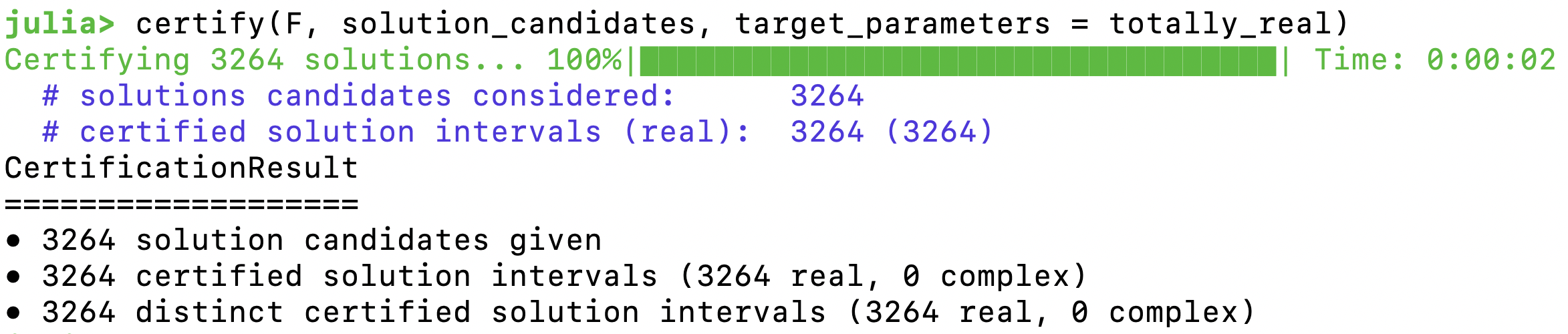
Figure 2: Screenshot from a Julia session, where we certify the 3264 real conics for the totally real arrangement from [BST20]. Here, F is the system of polynomials from (12) in [BST20]. The screenshot also demonstrates the simple syntax of our implementation.

5.2 Numerical Synthesis of Six-Bar Linkages

Now we demonstrate that the certification routine can cope with large problems. With our computation we improve a result from the literature.

We consider the kinematic synthesis of six-bar linkages that use eight prescribed accuracy points as described in [PM14]. In this article, the authors derive the synthesis equations for six-bar linkages of the Watt II, Stephenson II, and Stephenson III type. Additionally, in [PM14, Eq. (35)] they construct a system of 22 polynomials in 22 unknowns and 224 parameters, that can be used as a start system in a parameter homotopy to solve the synthesis equations of all three considered six-bar linkage types.

The number of non-singular zeros of this generalized start system is reported as 92,736. It was computed using Bertini and a multi-homogeneous start system. To certify the reported count, we solved the generalized start system using the monodromy method [DHJ⁺18] implementation in HomotopyContinuation.jl. In our computation we obtained 92,752 non-singular zeros for a generic choice of the 224 parameters. These are sixteen more than reported in [PM14]. We certified this count using our certification routine and obtained 92,752 distinct strong interval approximate zeros. Therefore, we have a certificate that the generalized system has in general (at least) 92,752 non-singular solution. This establishes that the result in [PM14] undercounts the true number of solutions. The certification needed only 38.34 seconds which underlines the scalability of the certification routine. Notice that the naive method for comparing intervals in Section 4.4 gives $4.301.420.376$ pairs to check. This underlines the need for having an efficient algorithm for comparing pairs.

6 Proof of the Krawczyk method

The idea for the proof of both Theorem 3.6 and Proposition 3.10 is to verify that for strong interval approximate zeros $I$ the map $G_{Y}(x)=x-Y\cdot F(x)$ defines a contraction on $I$. If this is true, by Banach’s Fixed Point Theorem there is exactly one fixed-point of this map in $I$. Since $Y$ is invertible, this implies that there is exactly one zero to $F(x)$ in $I$.

Before we give the proof of Theorem 3.6, we need a lemma. It is a direct sequence of a complex version of the mean-value theorem.

Lemma 6.1.

Let $Y\in\mathbb{C}^{n\times n}$ and $F:\mathbb{C}^{n}\to\mathbb{C}^{n}$. Define $G_{Y}(x)=x-YF(x)$. Let $I\in\mathbb{IC}^{n}$ be an interval vector and $x,z\in I$. Then, we have

1. $G_{Y}(z)-G_{Y}(x)\in(\mathbf{1}_{n}-Y\cdot\square\mathrm{J}F(I))\,\mathrm{Re}(z-x)+(\mathbf{1}_{n}-Y\cdot\square\mathrm{J}F(I))\,i\mathrm{Im}(z-x).$

2. $G_{Y}(I)\subset K_{x,Y}(I)$.

Proof.

The following proof is adapted from [BLL19, Lemma 2].

In the proof we abbreviate $G:=G_{Y}$. We first show the second part assuming the first part of the lemma. Then, we prove the first part. We fix an interval $I\in\mathbb{IC}^{n}$ and $x,z\in\mathbb{C}^{n}$.

For the second part, we have to show that for all $I\in\mathbb{IC}^{n}$ we have $G(I)\subset K_{x,Y}(I)$. To show this we define the interval matrix $M:=(\mathbf{1}_{n}-Y\square\mathrm{J}F(I))\in\mathbb{IC}^{n\times n}$. By definition of $K_{x,Y}$ we have $G(x)+M(I-x)\subset K_{x,Y}(I)$. Thus, we have to show that $G(z)-G(x)\in M(I-x)$, since $z\in I$ is arbitrary. The first part of the lemma implies that we can find matrices $M_{1},M_{2}\in M$ such that $G(z)-G(x)=M_{1}\mathrm{Re}(z-x)+iM_{2}\mathrm{Im}(z-x)$. Decomposing the matrices into real and imaginary part we find

$$G(z)-G(x)=\mathrm{Re}(M_{1})\mathrm{Re}(z-x)-\mathrm{Im}(M_{2})\mathrm{Im}(z-x)+i(\mathrm{Im}(M_{1})\mathrm{Re}(z-x)+\mathrm{Re}(M_{2})\mathrm{Im}(z-x)).$$

Since $z-x\in I$ and by definition of the complex interval multiplication from (2) and the interval matrix-vector-multiplication (3) we see that $G(z)-G(x)\in M(I-x)$. This finishes the proof for the second part.

The first part of the lemma may be shown entry-wise. We will show this by combining a complex version of the mean value theorem with the following observation: $\mathrm{J}G(x)=\mathbf{1}_{n}-Y\cdot\mathrm{J}F(x)$, so we have the inclusion

$$\mathrm{J}G(I)=\mathbf{1}_{n}-Y\cdot\mathrm{J}F(I)\subseteq\mathbf{1}_{n}-Y\cdot\square\mathrm{J}F(I).$$ (4)

We relate $G(z)-G(x)$ to (4) using the mean value theorem. First, we define $w:=\mathrm{Re}(z)+i\mathrm{Im}(x)$. Let $1\leq j\leq n$ and let $G_{j}$ denote the $j$-th entry of $G$. We define the function $h(t):=G_{j}(tz+(1-t)w)$. The real and imaginary part of $h(t)$ are real differentiable functions of the real variable $t$. The mean value theorem can be applied, and we find $0<t_{1},t_{2}<1$ such that $\mathrm{Re}(h(1))-\mathrm{Re}(h(0))=\tfrac{\mathrm{d}}{\mathrm{d}t}\mathrm{Re}(h(t_{1}))$ and $\mathrm{Im}(h(1))-\mathrm{Im}(h(0))=\frac{\mathrm{d}}{\mathrm{d}t}\mathrm{Im}(h(t_{2}))$. Setting $c_{1}=t_{1}z+(1-t_{1})w$ and $c_{2}=t_{2}z+(1-t_{2})w$ this implies

$$G_{j}(w)-G_{j}(z)=(\nabla_{\mathrm{Re}}\mathrm{Re}(G_{j}(c_{1})))^{T}(z-w)+i\nabla_{\mathrm{Re}}\mathrm{Im}(G(c_{2})))^{T}(z-w),$$

where $\nabla_{\mathrm{Re}}G$ denotes the vector of partial derivatives with respect to the real variable. Let us denote by $G_{j}^{\prime}$ the complex derivative of $G_{j}$; that is, $G_{j}^{\prime}:\mathbb{C}^{n}\to\mathbb{C}^{n}$ as a function. From the Cauchy Riemann equations it follows that $\nabla_{\mathrm{Re}}\mathrm{Re}(G_{j}(c_{1}))=\mathrm{Re}(G_{j}^{\prime}(c_{1}))$ and likewise $\nabla_{\mathrm{Re}}\mathrm{Im}(G(c_{2}))=\mathrm{Im}(G^{\prime}(c_{2}))$. This yields $G_{j}(z)-G_{j}(w)=(\mathrm{Re}(G_{j}^{\prime}(c_{1})+i\mathrm{Im}(G_{j}^{\prime}(c_{2})))^{T}(z-w)$. Putting these equations ranging over $j$ together we find $G(z)-G(w)=(\mathrm{Re}(\mathrm{J}G(c_{1}))+i\mathrm{Im}(\mathrm{J}G(c_{2})))(z-w)$. By construction, $c_{1}$ and $c_{2}$ are contained in $I$, because $w$ and $z$ are contained in $I$, and $I$ is a product of rectangles and thus convex. Combined with (4) this yields

$$G(z)-G(w)\in(\mathbf{1}_{n}-Y\cdot\square\mathrm{J}F(I))(z-w).$$

Using essentially the same arguments for the path from $x$ to $w$ we also find

$$G(w)-G(x)\in(\mathbf{1}_{n}-Y\cdot\square\mathrm{J}F(I))(w-x).$$

By construction, $z-w=i\mathrm{Im}(z-x)$ and $w-x=\mathrm{Re}(z-x)$, which implies

$$G(z)-G(x)\in(\mathbf{1}_{n}-Y\cdot\square\mathrm{J}F(I))\,\mathrm{Re}(z-x)+(\mathbf{1}_{n}-Y\cdot\square\mathrm{J}F(I))\,i\mathrm{Im}(z-x).$$

This finishes the proof. ∎

Proof of Theorem 3.6 and Proposition 3.10.

We fix $Y\in\mathbb{C}^{n\times n}$. The second part of Lemma 6.1 implies that, if we have $K_{x,Y}(I)\subseteq I$, then $G_{Y}(I)\subseteq I$. Brouwer’s fixed point Theorem shows that $G_{Y}$ has a fixed point in $I$. Since $Y$ is assumed to be invertible, the fixed point is a zero of $F$. This finishes the proof for the first part of Theorem 3.6. For the second part let $z_{0},z_{1}\in I$. The first part of Lemma 6.1 implies

$$G_{Y}(z_{0})-G_{Y}(z_{1})\in(\mathbf{1}_{n}-Y\cdot\square\mathrm{J}F(I))\text{Re}(z_{0}-z_{1})+(\mathbf{1}_{n}-Y\cdot\square\mathrm{J}F(I))\ i\text{Im}(z_{0}-z_{1}).$$

(Note that we can’t apply the distributivity law because of Theorem 2.1 3.). Applying norms and using submultiplicativity yields

$$\lVert G_{Y}(z_{0})-G_{Y}(z_{1})\rVert_{\infty}\leq\lVert(\mathbf{1}_{n}-Y\cdot\square\mathrm{J}F(I))\rVert_{\infty}\,(\lVert\text{Re}(z_{0}-z_{1})\rVert_{\infty}+\lVert\text{Im}(z_{0}-z_{1})\rVert_{\infty}).$$

Since $\lVert\text{Re}(z_{0}-z_{1})\rVert_{\infty}+\lVert\text{Im}(z_{0}-z_{1})\rVert_{\infty}\leq\sqrt{2}\lVert z_{0}-z_{1}\rVert_{\infty}$ it holds

$$\lVert G_{Y}(z_{0})-G_{Y}(z_{1})\rVert_{\infty}\leq\sqrt{2}\lVert\mathbf{1}_{n}-Y\cdot\square\mathrm{J}F(I)\rVert_{\infty}\lVert z_{0}-z_{1}\rVert_{\infty}.$$ (5)

By assumption $\sqrt{2}\lVert\mathbf{1}_{n}-Y\cdot\square\mathrm{J}F(I)\rVert_{\infty}$ is smaller than 1 so $G_{Y}$ is a contraction. Banach’s Fixed Point Theorem implies that $G_{Y}$ has a unique fixed point in $I$. Since $Y$ is invertible, this fixed point is the unique zero of $F$ in $I$. This shows the second part of Theorem 3.6.

Finally, let $(x_{i})_{i\geq 0}$ be the sequence defined in Proposition 3.10. By assumption, $x_{0}\in I$ and $x_{i+1}=G_{Y}(x_{i})$, $i\geq 0$. The second part of Lemma 6.1 together with an induction argument imply that $x_{i}\in I$ for all $i$. Let $x^{*}$ be the unique zero of $F$ in $I$. Then, 5 holds if we replace $z_{0}$ by $x^{*}$ and $z_{1}$ by $x_{i}$. We get $\lVert x^{*}-x_{i+1}\rVert_{\infty}<c\cdot\lVert x^{*}-x_{i}\rVert_{\infty}$ with a constant $c:=\sqrt{2}\lVert\mathbf{1}_{n}-Y\cdot\square\mathrm{J}F(I)\rVert_{\infty}<1$. This shows linear convergence and finishes the proof of Proposition 3.10. ∎

7 Certifying reality

For many applications only the real zeros of a polynomial system are of interest. Since numerical homotopy continuation computes in $\mathbb{C}^{n}$, it is important to have a rigorous method to determine whether a zero is real.

Recall from Definition 3.7 the notion of strong interval approximate zero.

Lemma 7.1.

Let $F:\mathbb{C}^{n}\rightarrow\mathbb{C}^{n}$ be a real square system of polynomials (or rational functions) and $I\in\mathbb{IC}^{n}$ a strong interval approximate zero of $F$. Then there exists $x\in I$ and $Y\in\mathbb{C}^{n\times n}$ satisfying $K_{x,Y}(I)\subset I$ and $\sqrt{2}\,\lVert\mathbf{1}_{n}-Y\square\mathrm{J}F(I)\rVert_{\infty}<1$. If additionally $\{\bar{z}\,|\,z\in K_{x,Y}(I)\}\subset I$, the associated zero of $I$ is real.

Proof.

Theorem 3.6 implies that $F$ has a unique zero $s\in K_{x,Y}(I)\subset I$. The element wise complex conjugate $\bar{s}$ is also a zero of $F$. If we have that $\bar{s}\in\{\bar{z}\,|\,z\in K_{x,Y}(I)\}\subset I$, then $\bar{s}=s$, since otherwise $\bar{s}$ and $s$ would be two distinct zeros of $F$ in $I$, contradicting the uniqueness result from Theorem 3.6. ∎

For a wide range of applications positive real zeros are of particular interest.

Corollary 7.2.

Let $F:\mathbb{C}^{n}\rightarrow\mathbb{C}^{n}$ be a real square system of polynomials and $I\in\mathbb{IC}^{n}$ a strong interval approximate zero of $F$ satisfying the conditions of Lemma 7.1. If $\textnormal{Re}(I)>0$ then the associated zero of $I$ is real and positive.

If the reality test in Lemma 7.1 fails for a strong interval approximate zero $I\in\mathbb{C}^{n}$ then this does not necessarily mean that the associated zero of $I$ is not real. A sufficient condition that $I$ is not real is that there is a coordinate such that the imaginary part of it does not contain zero.

Lemma 7.3.

Let $F(x)$ be a square system of polynomials or rational functions and let $I\in\mathbb{IC}^{n}$ be a strong interval approximate zero of $F$. If there exists $k\in\{1,\ldots,n\}$ such that $0\notin\mathrm{Im}(I_{k})$ then the associated zero of $I$ is not real.

Proof.

The associated zero $x$ of $I$ is contained in $I$. Since $0\notin\mathrm{Im}(I_{k})$ follows $x_{k}\notin\mathbb{R}$ and $x\notin\mathbb{R}^{n}$. ∎

Now assume that the certification routine produced a list $\mathcal{I}$ of $m$ distinct strong interval approximate zeros for a given system $F$, and that $m$ also agrees with the theoretical upper bound on the number of isolated, nonsingular zeros of $F$. If we apply Lemma 7.1 to $I_{k}\in\mathcal{I}$, then we obtain only a lower bound, say $r$, on the number of real zeros of $F$. However, combined with Lemma 7.3 we can also obtain an upper bound of the number of real zeros. If these two bounds agree we obtain a certificate that, among the associated zeros of the intervals in $\mathcal{I}$, there are exactly $r$ real zeros. An application of this is, e.g., the study of the distribution of the number of real solutions of the power flow equations [LZBL20].

References

- [ABF+21] Daniele Agostini, Taylor Brysiewicz, Claudia Fevola, Lukas Kühne, Bernd Sturmfels, and Simon Telen. Likelihood degenerations. arXiv preprint arXiv:2107.10518, 2021.
- [BCS13] Peter Bürgisser, Michael Clausen, and Mohammad A. Shokrollahi. Algebraic Complexity Theory, volume 315. Springer Science & Business Media, 2013.
- [BEKS17] Jeff Bezanson, Alan Edelman, Stefan Karpinski, and Viral B. Shah. Julia: A Fresh Approach to Numerical Computing. SIAM Review, 59(1):65–98, 2017.
- [BFS21] Taylor Brysiewicz, Claudia Fevola, and Bernd Sturmfels. Tangent quadrics in real 3-space. Le Matematiche, 76(2):355–367, 2021.
- [BHIM22] Paul Breiding, Reuven Hodges, Christian Ikenmeyer, and Mateusz Michałek. Equations for gl invariant families of polynomials. Vietnam Journal of Mathematics, pages 1–12, 2022.
- [BHSW] Daniel J. Bates, Jonathan D. Hauenstein, Andrew J. Sommese, and Charles W. Wampler. Bertini: Software for Numerical Algebraic Geometry. Available at bertini.nd.edu with permanent doi: dx.doi.org/10.7274/R0H41PB5.
- [BKK20] Taylor Brysiewicz, Khazhgali Kozhasov, and Mario Kummer. Nodes on quintic spectrahedra. arXiv preprint arXiv:2011.13860, 2020.
- [BLL19] Michael Burr, Kisun Lee, and Anton Leykin. Effective Certification of Approximate Solutions to Systems of Equations Involving Analytic Functions. In Proceedings of the 2019 on International Symposium on Symbolic and Algebraic Computation, ISSAC ’19, pages 267–274, New York, NY, USA, 2019. Association for Computing Machinery.
- [BPS21] Tobias Boege, Sonja Petrović, and Bernd Sturmfels. Marginal independence models. arXiv preprint arXiv:2112.10287, 2021.
- [BRST22] Paul Breiding, Felix Rydell, Elima Shehu, and Angélica Torres. Line multiview varieties. arXiv preprint arXiv:2203.01694, 2022.
-
[BS]
Luis Benet and David P. Sanders.
IntervalRootFinding.jl.
https://juliaintervals.github.io/IntervalRootFinding.jl. - [BST20] Paul Breiding, Bernd Sturmfels, and Sascha Timme. 3264 Conics in a Second. Notices of the American Mathematical Society, 67:30–37, 2020.
- [BSW21] Paul Breiding, Frank Sottile, and James Woodcock. Euclidean distance degree and mixed volume. Foundations of Computational Mathematics, 2021.
- [BT18] Paul Breiding and Sascha Timme. HomotopyContinuation.jl: A Package for Homotopy Continuation in Julia. In Mathematical Software – ICMS 2018, pages 458–465, Cham, 2018. Springer International Publishing.
- [BT21] Matías R Bender and Simon Telen. Yet another eigenvalue algorithm for solving polynomial systems. arXiv preprint arXiv:2105.08472, 2021.
- [CLL14] Tianran Chen, Tsung-Lin Lee, and Tien-Yien Li. Hom4PS-3: A Parallel Numerical Solver for Systems of Polynomial Equations Based on Polyhedral Homotopy Continuation Methods. In Hoon Hong and Chee Yap, editors, Mathematical Software – ICMS 2014, pages 183–190. Springer Berlin Heidelberg, 2014.
- [DHJ+18] Timothy Duff, Cvetelina Hill, Anders Jensen, Kisun Lee, Anton Leykin, and Jeff Sommars. Solving polynomial systems via homotopy continuation and monodromy. IMA Journal of Numerical Analysis, 39(3):1421–1446, 04 2018.
- [Ear21] Nick Early. Planarity in generalized scattering amplitudes: Pk polytope, generalized root systems and worldsheet associahedra. arXiv preprint arXiv:2106.07142, 2021.
- [GD05] Hatice Gecegormez and Yasar Demirel. Phase stability analysis using interval Newton method with NRTL model. Fluid Phase Equilibria, 237(1-2):48––58, 2005.
- [GS05] Balajit Gopalan and Jay-Dean Seader. Application of interval Newton’s method to chemical engineering problems. Reliable Computing, 1(3):215––223, 2005.
- [Hig02] Nicholas J. Higham. Accuracy and stability of numerical algorithms, volume 80. Siam, 2002.
- [HS95] Birkett Huber and Bernd Sturmfels. A polyhedral method for solving sparse polynomial systems. Math. Comp., 64(212):1541–1555, 1995.
- [HS12] Jonathan D. Hauenstein and Frank Sottile. Algorithm 921: alphaCertified: Certifying Solutions to Polynomial Systems. ACM Trans. Math. Softw., 38(4), Aug 2012.
- [Joh17] Frederik Johansson. Arb: efficient arbitrary-precision midpoint-radius interval arithmetic. IEEE Transactions on Computers, 66:1281–1292, 2017.
- [KPR+21] Kathlén Kohn, Ragni Piene, Kristian Ranestad, Felix Rydell, Boris Shapiro, Rainer Sinn, Miruna-Stefana Sorea, and Simon Telen. Adjoints and canonical forms of polypols. arXiv preprint arXiv:2108.11747, 2021.
- [Kra69] Rudolf Krawczyk. Newton-Algorithmen zur Bestimmung von Nullstellen mit Fehlerschranken. Computing, 4(3):187–201, 1969.
- [KSS15] Virendra Kumar, Soumen Sen, and Sankar Shome. Inverse Kinematics of Redundant Manipulator using Interval Newton Method. International Journal of Engineering and Manufacturing, 2:19––20, 2015.
- [LAR21] Julia Lindberg, Carlos Améndola, and Jose Israel Rodriguez. Estimating gaussian mixtures using sparse polynomial moment systems. arXiv preprint arXiv:2106.15675, 2021.
- [Lee19] Kisun Lee. Certifying approximate solutions to polynomial systems on Macaulay2. ACM Communications in Computer Algebra, 53(2):45–48, 2019.
- [Ley11] Anton Leykin. Numerical Algebraic Geometry for Macaulay2. The Journal of Software for Algebra and Geometry: Macaulay2, 3:5–10, 2011.
- [LZBL20] Julia Lindberg, Alisha Zachariah, Nigel Boston, and Bernard C. Lesieutre. The distribution of the number of real solutions to the power flow equations, 2020.
- [Mar21] Ivan A. Martyanov. Solving the delsarte problem for 4-designs on the sphere. Chebyshevskii Sb., 22:154–165, 2021.
- [May17] Günter Mayer. Interval Analysis. De Gruyter, Berlin, Boston, 2017.
- [Moo66] Ramon E. Moore. Interval Analysis, volume 4. Prentice-Hall, 1966.
- [Moo77] Ramon E. Moore. A Test for Existence of Solutions to Nonlinear Systems. SIAM Journal on Numerical Analysis, 14(4):611–615, 1977.
- [MS89] Alexander P. Morgan and Andrew J. Sommese. Coefficient-parameter polynomial continuation. Applied Mathematics and Computation, 29(2):123–160, 1989.
- [PM14] Mark M. Plecnik and John M. McCarthy. Numerical Synthesis of Six-Bar Linkages for Mechanical Computation. Journal of Mechanisms and Robotics, 6(3), 06 2014. 031012.
- [RTV97] Felice Ronga, Alberto Tognoli, and Thierry Vust. The number of conics tangent to five given conics: the real case. Rev. Mat. Univ. Complut. Madrid, 10:391–421, 1997.
- [Rum83] Siegfried M. Rump. Solving algebraic problems with high accuracy. In Proc. of the Symposium on A New Approach to Scientific Computation, page 51–120, USA, 1983. Academic Press Professional, Inc.
- [Rum99] Siegfried M. Rump. INTLAB - INTerval LABoratory. In Developments in Reliable Computing, pages 77–104. Kluwer Academic Publishers, 1999.
- [Rum10] Siegfried M. Rump. Verification methods: Rigorous results using floating-point arithmetic. Acta Numerica, 19:287–449, 2010.
- [Sma86] Steve Smale. Newton’s Method Estimates from Data at One Point. In Richard E. Ewing, Kenneth I. Gross, and Clyde F. Martin, editors, The Merging of Disciplines: New Directions in Pure, Applied, and Computational Mathematics, pages 185–196. Springer, 1986.
- [ST21] Bernd Sturmfels and Simon Telen. Likelihood equations and scattering amplitudes. Algebraic Statistics, 12(2):167–186, 2021.
- [Stu21] Bernd Sturmfels. Beyond linear algebra. arXiv preprint arXiv:2108.09494, 2021.
- [Sun58] Teruo Sunaga. Theory of an interval algebra and its application to numerical analysis. Research Association of Applied Geometry, 2:29–46, 1958.
- [SW05] Andrew Sommese and Charles Wampler. The Numerical Solution of Systems of Polynomials Arising in Engineering and Science. World Scientific, 2005.
- [SY21] Frank Sottile and Thomas Yahl. Galois groups in enumerative geometry and applications. arXiv preprint arXiv:2108.07905, 2021.
- [Ver99] Jan Verschelde. Algorithm 795: PHCpack: A General-Purpose Solver for Polynomial Systems by Homotopy Continuation. ACM Trans. Math. Softw., 25(2):251–276, June 1999.
- [Wei21] Madeleine Aster Weinstein. Metric Algebraic Geometry. University of California, Berkeley, 2021.