A Q-learning algorithm for discrete-time linear-quadratic control with random parameters of unknown distribution: convergence and stabilization

Abstract

This paper studies an infinite horizon optimal control problem for discrete-time linear systems and quadratic criteria, both with random parameters which are independent and identically distributed with respect to time. A classical approach is to solve an algebraic Riccati equation that involves mathematical expectations and requires certain statistical information of the parameters. In this paper, we propose an online iterative algorithm in the spirit of Q-learning for the situation where only one random sample of parameters emerges at each time step. The first theorem proves the equivalence of three properties: the convergence of the learning sequence, the well-posedness of the control problem, and the solvability of the algebraic Riccati equation. The second theorem shows that the adaptive feedback control in terms of the learning sequence stabilizes the system as long as the control problem is well-posed. Numerical examples are presented to illustrate our results.

1 Introduction and main results

This paper aims to propose an online algorithm to solve the infinite horizon linear quadratic (LQ) control problem for discrete-time systems with random parameters. Given an initial state $x_{0}=x\in\mathbb{R}^{n}$, the system evolves as

$$x_{t+1}=\varLambda_{t+1}\begin{bmatrix}x_{t}\\ u_{t}\end{bmatrix},\quad t=0,1,2,\dots,$$ (1.1)

where $x_{t}\in\mathbb{R}^{n}$ denotes the state and $u_{t}\in\mathbb{R}^{m}$ the control at time $t$; the cost function is defined as

$$J(x,u_{\cdot})=\sum_{t=0}^{\infty}\big{[}x_{t}^{\mathsf{T}},u_{t}^{\mathsf{T}}\big{]}N_{t+1}\begin{bmatrix}x_{t}\\ u_{t}\end{bmatrix}.$$ (1.2)

The random parameters $\varLambda_{t+1}$ and $N_{t+1}$ that affect the system from $t$ to $t+1$ are not exposed until time $t+1$. The objective of this control problem is to minimize the expected value of the cost function among all admissible controls; the selection of such a control $u_{t}$ is only based on the information of parameters up to time $t$. In this paper, we assume that $N_{t}$ is positive semidefinite, and the random matrices $[\varLambda_{t}^{\mathsf{T}},N_{t}]$ with $t=1,2,\dots$ are independent and identically distributed, but their statistical information is previously unknown. In what follows, $[\varLambda^{\mathsf{T}},N]$ denotes an independent copy of $[\varLambda_{1}^{\mathsf{T}},N_{1}]$.

The study of optimal control of discrete-time linear systems with independent random parameters can date back to Kalman [19] in 1961, motivated by random sampling systems [20]. Unsurprisingly, such models arise also in many other situations, for instance, control systems that involve state and control-dependent noise [12, 22, 16], digital control of diffusion processes [29], and macroeconomic systems [10, 3] where the randomness of parameters of econometric models is taken into account.

Due to the wide application background, the LQ problem with random parameters has been extensively studied (see [19, 12, 1, 5, 21, 11, 23, 35, 25, 6, 17, 32] for example). As far as the infinite horizon problem is concerned, the key issues addressed mostly in the literature include:

• to determine whether the LQ problem is well-posed, i.e., the value function

  $$V(x):=\inf_{u_{\cdot}}\mathbb{E}[J(x,u_{\cdot})]~{}~{}~{}~{}~{}~{}~{}~{}~{}~{}~{}~{}$$ (1.3)

  is finite for all $x\in\mathbb{R}^{n}$; and if it is well-posed,

• to construct an optimal control $u_{\cdot}^{\star}$ for each $x$ such that $\mathbb{E}[J(x,u_{\cdot}^{\star})]=V(x)$.

Moreover, it is known that the well-posedness issue has an intimate link to stabilizability of the system (1.1) which in itself is an important topic and has also been widely discussed (see [22, 21, 11, 23, 34] for example).

For the above issues, a commonly used approach in the literature is to apply stochastic dynamic programming [2] to the LQ problem, resulting in an algebraic Riccati equation (ARE) that characterizes the value function and the optimal (feedback) control. In this sense, the problem can be perfectly solved if the distribution of the random parameters are known. To capture more mathematical insights, let us quickly look at the informal derivation. The value function, if it is finite, is believed to be a quadratic form, say, $V(x)=x^{\mathsf{T}}Kx$ with some positive semidefinite matrix $K$, then Bellman’s principle of optimality gives that

$$x^{\mathsf{T}}Kx =\inf_{u_{t}}\mathbb{E}\bigg{\{}\big{[}x_{t}^{\mathsf{T}},u_{t}^{\mathsf{T}}\big{]}N_{t+1}\begin{bmatrix}x_{t}\\ u_{t}\end{bmatrix}+x_{t+1}^{\mathsf{T}}Kx_{t+1}\,\bigg{|}\,x_{t}=x\bigg{\}}$$ (1.4)

$$=\inf_{u_{t}}\mathbb{E}\bigg{\{}\big{[}x_{t}^{\mathsf{T}},u_{t}^{\mathsf{T}}\big{]}(N_{t+1}+\varLambda_{t+1}^{\mathsf{T}}K\varLambda_{t+1})\begin{bmatrix}x_{t}\\ u_{t}\end{bmatrix}\bigg{|}\,x_{t}=x\bigg{\}}$$

$$=\min_{u\in\mathbb{R}^{m}}\big{[}x^{\mathsf{T}},u^{\mathsf{T}}\big{]}\big{(}\mathbb{E}[N_{t+1}+\varLambda_{t+1}^{\mathsf{T}}K\varLambda_{t+1}]\big{)}\begin{bmatrix}x\\ u\end{bmatrix}\quad\forall\,x\in\mathbb{R}^{n};$$

the last unconditional extremum can be solved out explicitly. To proceed further, let us introduce some notations used frequently in this paper. Let $\mathbb{S}_{+}^{d}$ be the set of positive semidefinite $d\times d$-matrices with $d=n+m$, and for any $P\in\mathbb{S}_{+}^{d}$ we refer to its certain submatrices according to the following partition:

$$P=\begin{bmatrix}P_{xx}&P_{xu}\\ P_{ux}&P_{uu}\end{bmatrix}\quad\text{with }\ P_{xx}\in\mathbb{R}^{n\times n},$$ (1.5)

and define the following two mappings:

$$\Pi(P) :=P_{xx}-P_{xu}P_{uu}^{+}P_{ux},$$ (1.6)

$$\Gamma(P) :=-P_{uu}^{+}P_{ux},$$

where $P_{uu}^{+}$ denotes the Moore–Penrose pseudoinverse of $P_{uu}$. Using the above notations, one can easily obtain from (1.4) that

$$K=\Pi(\mathbb{E}[N+\varLambda^{\mathsf{T}}K\varLambda]),$$ (1.7)

which is exactly the algebraic Riccati equation (ARE) for LQ problem (1.1)–(1.2). Moreover, the infimum in (1.4) can be achieved by taking

$$u_{t}=\Gamma(\mathbb{E}[N+\varLambda^{\mathsf{T}}K\varLambda])x_{t},$$

which gives the optimal feedback control of the LQ problem. In principle, to compute the expectation in (1.7) one need know certain statistical information of the parameters $N_{t}$ and $\varLambda_{t}$.

The above argument can be rigorized without much effort; actually, under rather general settings, LQ problem (1.1)–(1.2) is well-posed if and only if ARE (1.7) has a solution (see [11, 23] or Theorem 1 below). Utilizing this relation, some useful criteria for well-posedness of infinite horizon LQ problems are obtained in the papers [12, 5, 21, 11] under various circumstances where the mathematical expectation in ARE (1.7) can be evaluated accurately.

A natural question is, how to solve LQ problem (1.1)–(1.2) when the statistical information of the parameters is inadequate and ARE (1.7) fails to work.

In this paper we propose a Q-learning algorithm to tackle this question. Q-learning is a value-based reinforcement learning algorithm which is used to find the optimal control policy using a state-control value function, called the Q-function or Q-factor, instead of the usual value function in dynamic programming; see [7, 28]. The original and most widely known Q-learning algorithm of Watkins [33] is a stochastic version of value iteration, applying to Markov decision problems with unknown costs and transition probabilities. The starting point is to reformulate Bellman’s equation into an equivalent form that is particularly convenient for deriving learning algorithm. Let us briefly illustrate how this works in our case. Defining

$$Q^{*}=\mathbb{E}[N+\varLambda^{\mathsf{T}}K\varLambda]\in\mathbb{R}^{d\times d},$$

ARE (1.7) are equivalent to the following equation:

$$Q^{*}=\mathbb{E}[N+\varLambda^{\mathsf{T}}\Pi(Q^{*})\varLambda].$$ (1.8)

The mathematical convenience of this reformulation derives from the fact that the nonlinear operator $\Pi(\cdot)$ appears inside the expectation in (1.8), whereas it appears outside the expectation in ARE (1.7). This fact plays an important role in the feasibility and convergence of Q-learning algorithms.

Algorithm 1 Q-learning for LQ problem with random parameters

1:  Set the initial matrix $Q_{0}$.

2:  while not converged do

3:     $Q_{t+1}\leftarrow Q_{t}+\alpha_{t}(N_{t+1}+\varLambda_{t+1}^{\mathsf{T}}\Pi(Q_{t})\varLambda_{t+1}-Q_{t})$.

4:  end while

Algorithm 1 presented above is our Q-learning algorithm for LQ problem (1.1)–(1.2), where the learning rate sequence $(\alpha_{t}\in[0,1]:t=0,1,\dots)$ satisfies

$$\sum_{t=0}^{\infty}\alpha_{t}=\infty\quad\text{and}\quad\sum_{t=0}^{\infty}\alpha_{t}^{2}<\infty,$$ (1.9)

which can be random as long as $\alpha_{t}$ is measurable to $\sigma\{\varLambda_{s},N_{s}:s=1,\dots,t\}$. The objective of this algorithm is to learn the matrix $Q^{*}$ (if it exists) that solves (1.8), based on the observed samples of the parameters.

Algorithm 1 is an online learning algorithm. As pointed out by Tsitsiklis [31], the Q-learning algorithm is recursive and each new piece of information of the parameters is immediately used for computing an additive correction term to the old estimates. The iteration in Algorithm 1, i.e.,

$$Q_{t+1}=Q_{t}+\alpha_{t}(N_{t+1}+\varLambda_{t+1}^{\mathsf{T}}\Pi(Q_{t})\varLambda_{t+1}-Q_{t})$$ (1.10)

can be regarded as a stochastic version of the standard fixed-point iteration based on the equation (1.8).

The first theorem of this paper draws a full picture of the relationship among the LQ problem, ARE, and the Q-learning algorithm.

Theorem 1.

Let $(Q_{t})_{t\geq 0}$ be the sequence constructed in Algorithm 1. In addition to the above setting, we assume that $\mathbb{E}[\|N\|_{2}^{2}+\|\varLambda^{\mathsf{T}}\varLambda\|_{2}^{2}]$ is finite and $\mathbb{E}[N]$ is positive definite.

Then, the following statements are equivalent:

1. LQ problem (1.1)–(1.2) is well-posed;

2. ARE (1.7) admits a solution $K$;

3. $(Q_{t})_{t\geq 0}$ is bounded with a positive probability;

4. $(Q_{t})_{t\geq 0}$ converges almost surely (a.s.) to a deterministic matrix $Q^{\star}\in\mathbb{S}_{+}^{d}$.

Moreover, if either statement is valid, one has the following properties:

1. the value function $V(x)=x^{\mathsf{T}}Kx$ for all $x\in\mathbb{R}^{n}$;

2. the solution of ARE (1.7) is unique and given by $K=\Pi(Q^{\star})$;

3. the optimal control is given by feedback form $u_{t}^{\star}=\Gamma(Q^{\star})x_{t}$;

4. $Q^{\star}$ satisfies (1.8), i.e., $Q^{\star}=\mathbb{E}[N+\varLambda^{\mathsf{T}}\Pi(Q^{\star})\varLambda]$,

where the mappings $\Pi(\cdot)$ and $\Gamma(\cdot)$ are defined in (1.6).

In the theorem, we use $\|\cdot\|_{2}$ to denote the $2$-norm of Matrix. It is worth noting that statement (c) in this theorem looks relatively weak, but it still implies the convergence of $Q_{t}$ and the well-posedness of the LQ problem. Form above theorem, the sequence $Q_{t}$ is either convergent or divergent with probability 1. So we have

Corollary 2.

The probability that $(Q_{t})_{t\geq 0}$ is bounded is either $0$ or $1$.

This zero-one law endows the algorithm with great applicability. Indeed, this proves, at least theoretically, that just running or stimulating the system for one sample trajectory, we can almost certainly detect whether the LQ problem is well-posed or not, and also obtain the desired matrix $Q^{\star}$ if it exists.

The next theorem concerns the stabilization of system (1.1). We say system (1.1) is stabilizable a.s. if under some control the state vanishes a.s. as time tends to infinity. In terms of the sequence $Q_{t}$ from Algorithm 1, it is natural to construct an adaptive feedback control

$$u_{t}^{\mathrm{a}}=\Gamma(Q_{t})x_{t}.$$ (1.11)

It will be shown that this control stabilizes the system a.s. as long as the LQ problem is well-posed.

Theorem 3.

Under the same setting of Theorem 1, if LQ problem (1.1)–(1.2) is well-posed, then the state $x_{t}^{{\rm a}}$ under the control $u_{t}^{\mathrm{a}}$ satisfies

$$J(x,u_{\cdot}^{\mathrm{a}})<\infty\quad\text{and}\quad\sum_{t=0}^{\infty}\big{(}|x_{t}^{\mathrm{a}}|^{2}+|u_{t}^{\mathrm{a}}|^{2}\big{)}<\infty$$ (1.12)

a.s. for any initial state $x\in\mathbb{R}^{n}$; consequently, the adaptive feedback control $u_{\cdot}^{\mathrm{a}}$ given by (1.11) stabilizes system (1.1) a.s.

The stabilization in this result is in the path-wise sense, whereas a relevant definition widely used in the literature is called the mean-square stabilization, i.e., the second-order moment of the state, $\mathbb{E}[\|x_{t}\|_{2}^{2}]$, tends to zero under certain control (see [11, 34] from example). Either of these two definitions cannot cover each other, while the path-wise one is relatively suitable in our setting because our learning algorithm is carried out along one single sample path. Nevertheless, certain modification of the adaptive feedback control (1.11) may stabilize the system in these two sense simultaneously; one possible way is to cut-off the feedback coefficient $\Gamma(Q_{t})$ when its norm is larger than some given bound. The details are left to interested readers.

Let us give some remarks from the technical aspect. Like the original Q-learning, our algorithm can also be embedded into a broad class of stochastic approximation algorithms studied in [18, 31], two celebrated papers that give rigorous convergence proofs of the original Q-learning. However, the results in those papers cannot apply to Algorithm 1 directly for two reasons: firstly, they all require certain contraction conditions which are not satisfied in our case, and secondly, the partial order of vectors used in [31] are substantially different from that of symmetric matrices, so the monotonicity condition required there is not satisfied either. In the proof of Theorem 1 we adopt the comparison argument from [31]. The crucial fact we used is the monotonicity property of $\Pi(\cdot)$, which helps us construct upper and lower bounds for $Q_{t}$ from ARE on the one hand, and an upper bound for the approximating sequence of ARE from $Q_{t}$ on the other hand. The equivalence of statements (a) and (b), i.e., the well-posdness of LQ problem and the solvability of ARE, is proved by means of Bellman’s principle of optimality; similar results can be found in [11, 23] where the control is restricted in the feedback form.

The conditions of our results are quite general. The positive definiteness of $\mathbb{E}[N]$ can be weakened to some extent (see Remark 15), which ensures the same property of the solution of ARE and the limit $Q^{\star}$ (in this case the pseudoinverses in (1.7) and $\Pi(Q^{\star})$ are the standard matrix inverses). The finiteness of $\mathbb{E}[\|N\|_{2}^{2}+\|\varLambda^{\mathsf{T}}\varLambda\|_{2}^{2}]$ is a natural condition to prove the convergence of Algorithm 1 by use of some classical results from stochastic approximation theory. In applications, the verification of these conditions may depend on certain qualitative properties of specific systems rather than the full statistical information of parameters. For example, the conditions are automatically satisfied if $\varLambda,N$ are bounded and $N$ is positive definite a.s. Numerical examples are presented in Section 5. Nevertheless, it would be interesting to extend the results to the indefinite case, in which the matrix $N$ is not necessarily positive semidefinite. The indefinite LQ problem has applications in many fields such as robust control, mathematical finance, and so on; for more details, we refer the reader to [27, 9, 26, 24].

As far as LQ problems with unknown parameters are concerned, our approach is different from the well-known adaptive control [4] in some respects. First, the types of randomness are different: the noise in our model is multiplicative and has no specific structure, whereas most of control systems studied in adaptive control are perturbed by additive noise, for example, the linear–quadratic–Gaussian control problem (see [8, 13, 15, 4] and references therein); as for multiplicative noise, the adaptive control algorithms proposed in [1, 30], of which the convergence are not proved, still specify the type of noise and how it enters into the system. Second, a typical adaptive control algorithm consists of two parts: parameter estimation (or system identification) and control law, while in our approach we do not pursuit to identify the system but directly learn the state-control value function that yields the value function and control law. Nevertheless, an adaptive control algorithm usually makes use of the inputs and outputs of the system, but not the direct observation of the sample of parameters as we do in this paper. Obviously, in a period $[t,t+1]$, the information of inputs and outputs is often insufficient to determine the exact value of the sample of parameters. Modification of our algorithm based on inputs and outputs is expected in future work.

The rest of this paper is organized as follows. Section 2 presents some auxiliary lemmas. The whole of Section 3 is devoted to the proof of Theorem 1, split into five subsections. Section 4 gives the proof of Theorem 3. Numerical examples and further discussion are presented in Section 5.

2 Auxiliary lemmas

Let us introduce some notations used in what follows. For a vector $x$ and a matrix $M$, $|x|$ and $\|M\|_{2}$ denote their $2$-norms, respectively. For two symmetric matrices $M_{1},M_{2}$ with the same size, we write $M_{1}\geq M_{2}$ (resp. $M_{1}>M_{2}$) if $M_{1}-M_{2}$ is positive semidefinite (resp. definite); the notations $M_{1}\leq M_{2}$ and $M_{1}<M_{2}$ are similarly understood. $I_{n}$ denotes the $n\times n$ identity matrix, and $O$ the zero matrix whose size is determined by the context.

Lemma 4.

For any $Q_{1},Q_{2}\in\mathbb{S}_{+}^{d}$, we have

$$\Pi(Q_{1}+Q_{2})\geq\Pi(Q_{1})+\Pi(Q_{2}).$$ (2.1)

In particular, if $Q_{1}\leq Q_{2}$ then $\Pi(Q_{1})\leq\Pi(Q_{2})$.

Proof.

Recalling the definition of $\Pi(\cdot)$ in (1.6), one has that

$$\min_{v\in\mathbb{R}^{m}}\begin{bmatrix}\begin{array}[]{l}x\\ v\end{array}\end{bmatrix}^{\mathsf{T}}Q\begin{bmatrix}\begin{array}[]{l}x\\ v\end{array}\end{bmatrix}=x^{\mathsf{T}}\Pi(Q)x,\quad\forall\,Q\in\mathbb{S}_{+}^{d},\,x\in\mathbb{R}^{d},$$ (2.2)

which implies

$$x^{\mathsf{T}}\Pi(Q_{1}+Q_{2})x\geq x^{\mathsf{T}}\Pi(Q_{1})x+x^{\mathsf{T}}\Pi(Q_{2})x.$$

So (2.1) is proved.

Notice that $\Pi(Q)\geq O$ for any $Q\in\mathbb{S}_{+}^{d}$. If $Q_{1}\leq Q_{2}$, then

$$\Pi(Q_{2})\geq\Pi(Q_{1})+\Pi(Q_{2}-Q_{1})\geq\Pi(Q_{1}).$$

This concludes the proof. ∎

The coming result about a deterministic recursion is elementary.

Lemma 5.

Let $(f_{t}:t=0,1,2,\dots)$ be a bounded real valued sequence, and $(\beta_{t})\subset[0,1]$ satisfy $\sum_{t}\beta_{t}=\infty$. Suppose the sequence $y_{t}$ satisfies

$$y_{t+1}\leq(1-\beta_{t})y_{t}+\beta_{t}f_{t}.$$

Then

$$\limsup_{t\to\infty}y_{t}\leq\limsup_{t\to\infty}f_{t}.$$

Proof.

Let $\tilde{f}_{t}=\sup_{s\geq t}f_{s}$. Then $\tilde{f}_{t}\geq f_{t}$ and $\tilde{f}_{t}\geq\tilde{f}_{t+1}$ for all $t=0,1,2,\dots$ Also, define a sequence $(\tilde{y}_{t})$ with $\tilde{y}_{0}=|y_{0}|+|\tilde{f}_{0}|$ and

$$\tilde{y}_{t+1}=(1-\beta_{t})\tilde{y}_{t}+\beta_{t}\tilde{f}_{t}.$$ (2.3)

It follows from induction that

$$\tilde{y}_{t}\geq y_{t}\quad\text{and}\quad\tilde{f}_{t}\leq\tilde{y}_{t}.$$

Moreover, since $\tilde{y}_{t+1}$ is a convex combination of $\tilde{y}_{t}$ and $\tilde{f}_{t}$, one has $\tilde{y}_{t+1}\leq\tilde{y}_{t}$. Therefore, $\tilde{y}_{t}$ and $\tilde{f}_{t}$ are both decreasing and convergent. Because the sequence

$$z_{t}:=\tilde{y}_{0}-\tilde{y}_{t+1}=\sum_{s=0}^{t}\beta_{s+1}(\tilde{y}_{s}-\tilde{f}_{s})$$

is uniformly bounded, plus the facts that $\tilde{y}_{s}-\tilde{f}_{s}$ is non-negative and $\sum_{s}\beta_{s}=\infty$, there is subsequence $\{t^{\prime}\}$ from $\{t\}$ such that

$$\lim_{t^{\prime}\to\infty}(\tilde{y}_{t^{\prime}}-\tilde{f}_{t^{\prime}})=0,$$

which implies that $\tilde{y}_{t}$ and $\tilde{f}_{t}$ enjoy the same limit. So

$$\limsup_{t\to\infty}f_{t}=\lim_{t\to\infty}\tilde{f}_{t}=\lim_{t\to\infty}\tilde{y}_{t}\geq\limsup_{t\to\infty}y_{t}.$$

The proof is complete. ∎

The following two results of stochastic approximation are important in our argument.

Lemma 6.

Let $\{\mathcal{F}_{t}:t=0,1,2,\dots\}$ be a filtration on a probability space $(\Omega,\mathcal{F},\mathbb{P})$, and for each $t$, let $r_{t}$ and $\alpha_{t}$ be $\mathcal{F}_{t}$-adapted scalar processes, where $\alpha_{t}\in[0,1]$ satisfies (1.9). Suppose that there is an increasing sequence of stopping times $(\tau_{k}:k=1,2,\dots)$ such that

1. $\mathbb{P}(\sup_{k}\tau_{k}=\infty)>0$;

2. $\mathbb{E}[\mathbf{1}_{\{t<\tau_{k}\}}r_{t+1}|\mathcal{F}_{t\wedge\tau_{k}}]=0$ for all $t,k$;

3. $\mathbb{E}[\mathbf{1}_{\{t<\tau_{k}\}}r_{t+1}^{2}\big{|}\mathcal{F}_{t\wedge\tau_{k}}]\leq\mu_{k}$ a.s. with a sequence of deterministic numbers $\mu_{k}$.

Let $w_{t}$ satisfy the recursion:

$$w_{t+1}=(1-\alpha_{t})w_{t}+\alpha_{t}r_{t+1},\quad t=0,1,2\dots$$

Then $\lim_{t\to\infty}w_{t}=0$ on $\{\sup_{k}\tau_{k}=\infty\}$ a.s.

Proof.

First of all, we assume that $\mathbb{E}[r_{t+1}|\mathcal{F}_{t}]=0$ and $\mathbb{E}[r_{t+1}^{2}|\mathcal{F}_{t}]\leq\mu$ a.s. with some number $\mu$. Then convergence of $w_{t}$ follows from some classical results in stochastic approximation theory, e.g., Dvoretzky’s extended theorem [14].

Now for any $k\geq 0$, define $r_{t}^{k}=\mathbf{1}_{\{t<\tau_{k}\}}r_{t}$ and $\mathcal{F}_{t}^{k}=\mathcal{F}_{t\wedge\tau_{k}}$. Then from the assumptions and the above argument, the sequence $w_{t}^{k}$ constructed by

$$w_{t+1}^{k}=(1-\alpha_{t})w_{t}^{k}+\alpha_{t}r_{t+1}^{k},\quad w_{0}^{k}=w_{0}$$

converges to zero a.s. Notice that $w_{t}^{k}=w_{t}$ for all $t<\tau_{k}$, so we have $\lim_{t\to\infty}w_{t}=0$ on $\{\sup_{k}\tau_{k}=\infty\}$ a.s. ∎

Lemma 7.

Let $\alpha_{t}$ be a $[0,1]$-valued process adapted to a filtration $\mathcal{F}_{t}$ and satisfy (1.9), and let $R_{t}$ be an $\mathcal{F}_{t}$-adapted process with values in a vector space equipped with norm $\|\cdot\|$. Then the iterative process

$$X_{t+1}=(1-\alpha_{t})X_{t}+\alpha_{t}R_{t+1}$$

converges to zero a.s. under the following assumptions:

1. $\|\mathbb{E}[R_{t+1}|\mathcal{F}_{t}]\|\leq\lambda\|X_{t}\|$ a.s. with some constant $\lambda<1$,

2. $\mathbb{E}[\|R_{t+1}\|^{2}|\mathcal{F}_{t}]\leq\mu_{t}$ a.s., where $\mu_{t}\in\mathcal{F}_{t}$ and $\mathbb{P}\{\sup_{t}|\mu_{t}|<\infty\}=1$.

Proof.

By means of stopping skill, it suffices to prove the lemma with $\mu_{k}$ dominated by a constant $\mu$. Let

$$S_{t+1}=R_{t+1}-\mathbb{E}[R_{t+1}|\mathcal{F}_{t}].$$

Applying Lemma 6, one has that the vector sequence $W_{t}$ defined by

$$W_{t+1}=(1-\alpha_{t})W_{t}+\alpha_{t}S_{t+1}$$

converges to zero a.s. Setting $Y_{t}=X_{t}-W_{t}$, then

$$\|Y_{t+1}\| =\|(1-\alpha_{t})Y_{t}+\alpha_{t}\mathbb{E}[R_{t+1}|\mathcal{F}_{t}]\|$$

$$\leq(1-\alpha_{t})\|Y_{t}\|+\lambda\alpha_{t}\|Y_{t}+W_{t}\|$$

$$\leq[1-(1-\lambda)\alpha_{t}]\|Y_{t}\|+(1-\lambda)\alpha_{t}\frac{\lambda}{1-\lambda}\|W_{t}\|.$$

From Lemma 5 it follows that

$$\limsup_{t\to\infty}\|Y_{t}\|\leq\frac{\lambda}{1-\lambda}\lim_{t\to\infty}\|W_{t}\|=0\quad\text{a.s.}$$

This concludes the lemma. ∎

3 Proof of Theorem 1

It is easily seen that (d) $\Rightarrow$ (c). In the coming five subsections, we shall prove the relations (a) $\Rightarrow$ (b), (b) $\Rightarrow$ (a), (b) $\Rightarrow$ (c), (c) $\Rightarrow$ (b), and (c) $\Rightarrow$ (d), respectively.

Let us do some preparations. Recall that $[\varLambda_{t}^{\mathsf{T}},N_{t}]$ with $t=1,2,\dots$ are independent and identically distributed matrix-valued random variables on a probability space $(\Omega,\mathcal{F},\mathbb{P})$, and $[\varLambda^{\mathsf{T}},N]$ denotes an independent copy of $[\varLambda_{1}^{\mathsf{T}},N_{1}]$. Introduce the filtration $(\mathcal{F}_{t})$ with $\mathcal{F}_{0}=\{\varnothing,\Omega\}$ and

$$\mathcal{F}_{t}=\sigma\{\varLambda_{s},N_{s}:s=1,\dots,t\},\quad t=1,2,\dots.$$

Also recall that the control sequence is allowed to be any $\mathcal{F}_{t}$-adapted process in $\mathbb{R}^{m}$ (not necessarily of feedback form).

It is convenient to define two mappings

$$\Phi_{t}(Q) :=N_{t}+\varLambda_{t}^{\mathsf{T}}\Pi(Q)\varLambda_{t},$$ (3.1)

$$\Phi(Q) :=\mathbb{E}[N+\varLambda^{\mathsf{T}}\Pi(Q)\varLambda]$$

for $Q\in\mathbb{S}_{+}^{d}$; apparently, $\Phi(Q)=\mathbb{E}[\Phi_{t}(Q)]$.

An important fact is that $\Phi_{t}(\cdot)$ and $\Phi(\cdot)$ are both increasing, i.e., if $Q_{1}\leq Q_{2}$ then $\Phi_{t}(Q_{1})\leq\Phi_{t}(Q_{2})$ and $\Phi(Q_{1})\leq\Phi(Q_{2})$. This follows from the monotonicity of $\Pi(\cdot)$, see Lemma 4.

Occasionally, $\varLambda_{t}\in\mathbb{R}^{n\times d}$ is written into a block matrix $\varLambda_{t}=[A_{t},B_{t}]$ with $A_{t}\in\mathbb{R}^{n\times n}$, then the system reads

$$x_{t+1}=A_{t+1}x_{t}+B_{t+1}u_{t}.$$ (3.2)

From the condition of Theorem 1, there are two numbers $\varepsilon_{0}\in(0,1]$ and $\mu_{0}>0$ such that

$$\mathbb{E}[N+\varLambda^{\mathsf{T}}\varLambda]\geq\varepsilon_{0}I_{d},\quad\mathbb{E}[\|N\|_{2}^{2}+\|\varLambda^{\mathsf{T}}\varLambda\|_{2}^{2}]\leq\mu_{0}.$$ (3.3)

Finally, we claim that, if $u_{t}\in L^{2}(\Omega)$ for all $t$, then $x_{t}\in L^{2}(\Omega)$ for all $t$. Indeed, assuming $x_{t}\in L^{2}(\Omega)$ we compute

$$\mathbb{E}[|x_{t+1}|^{2}|\mathcal{F}_{t}] =\mathbb{E}\bigg{\{}\big{[}x_{t}^{\mathsf{T}},u_{t}^{\mathsf{T}}\big{]}\varLambda_{t+1}^{\mathsf{T}}\varLambda_{t+1}\begin{bmatrix}x_{t}\\ u_{t}\end{bmatrix}\bigg{|}\mathcal{F}_{t}\bigg{\}}$$

$$=\big{[}x_{t}^{\mathsf{T}},u_{t}^{\mathsf{T}}\big{]}(\mathbb{E}[\varLambda_{t+1}^{\mathsf{T}}\varLambda_{t+1}])\begin{bmatrix}x_{t}\\ u_{t}\end{bmatrix}$$

$$\leq c(\mu_{0})(|x_{t}|^{2}+|u_{t}|^{2}),$$

thus, $\mathbb{E}[\|x_{t+1}\|^{2}]<\infty$. The claim is so verified by induction. This ensures the well-posedness of the LQ problem in finite horizon.

3.1 From LQ problem to ARE

Consider the optimal control in finite horizon: let $T$ be a large natural number and define

$$V_{T}(x,t)=\inf_{u_{t},\dots,u_{T-1}}\mathbb{E}\bigg{\{}\sum_{s=t}^{T-1}\big{[}x_{s}^{\mathsf{T}},u_{s}^{\mathsf{T}}\big{]}N_{s+1}\begin{bmatrix}x_{s}\\ u_{s}\end{bmatrix}\,\bigg{|}\,x_{t}=x\bigg{\}}.$$

Recalling (1.3) the value function $V(\cdot)$ of the original problem, it is easily seen that

$$V_{T}(x,t)\leq V(x)\quad\forall\,x\in\mathbb{R}^{n},\,t=0,1,\dots,T-1.$$

For this finite horizon problem, it follows from Bellman’s principle of optimality (cf. [Aoki, p. 32]) that

$$V_{T}(x,t) =\inf_{u_{t}}\mathbb{E}\bigg{\{}\big{[}x_{t}^{\mathsf{T}},u_{t}^{\mathsf{T}}\big{]}N_{t+1}\begin{bmatrix}x_{t}\\ u_{t}\end{bmatrix}+V_{T}(x_{t+1},t+1)\,\bigg{|}\,x_{t}=x\bigg{\}}$$

for $t=0,1,\dots,T-1$; in particular, we set $V_{T}(x,T)=0$. Assume that $V_{T}(x,t+1)$ is a quadratic form for some $t\leq T-1$, namely,

$$V_{T}(x,t+1)=x^{\mathsf{T}}\mathcal{K}_{t+1,T}x,\quad\text{where }\mathcal{K}_{t+1,T}\text{ is a symmetric matrix}.$$

Then $V_{T}(x,t)$ is also a quadratic form:

$$V_{T}(x,t) =\inf_{u_{t}}\mathbb{E}\bigg{\{}\big{[}x_{t}^{\mathsf{T}},u_{t}^{\mathsf{T}}\big{]}N_{t+1}\begin{bmatrix}x_{t}\\ u_{t}\end{bmatrix}+\big{[}x_{t}^{\mathsf{T}},u_{t}^{\mathsf{T}}\big{]}\varLambda_{t+1}^{\mathsf{T}}\mathcal{K}_{t+1,T}\varLambda_{t+1}\begin{bmatrix}x_{t}\\ u_{t}\end{bmatrix}\,\bigg{|}\,x_{t}=x\bigg{\}}$$

$$=\inf_{u_{t}}\mathbb{E}\bigg{\{}\big{[}x^{\mathsf{T}},u_{t}^{\mathsf{T}}\big{]}\big{(}N_{t+1}+\varLambda_{t+1}^{\mathsf{T}}\mathcal{K}_{t+1,T}\varLambda_{t+1}\big{)}\begin{bmatrix}x\\ u_{t}\end{bmatrix}\bigg{\}}$$

$$=\inf_{u\in\mathbb{R}^{m}}\big{[}x^{\mathsf{T}},u^{\mathsf{T}}\big{]}\mathbb{E}[N_{t+1}+\varLambda_{t+1}^{\mathsf{T}}\mathcal{K}_{t+1,T}\varLambda_{t+1}]\begin{bmatrix}x\\ u\end{bmatrix}$$

$$=x^{\mathsf{T}}\Pi(\mathbb{E}[N_{t+1}+\varLambda_{t+1}^{\mathsf{T}}\mathcal{K}_{t+1,T}\varLambda_{t+1}])x$$

$$=:x^{\mathsf{T}}\mathcal{K}_{t,T}x.$$

By induction, one has

$$V_{T}(x,t)=x^{\mathsf{T}}\mathcal{K}_{t,T}x\quad\forall\,t=0,1,\dots,T,$$ (3.4)

where the matrices $\mathcal{K}_{t,T}$ satisfy the following algebraic Riccati equations:

$$\mathcal{K}_{t,T}=\Pi(\mathbb{E}[N+\varLambda^{\mathsf{T}}\mathcal{K}_{t+1,T}\varLambda]),\quad\mathcal{K}_{T,T}=O.$$ (3.5)

The following result shows that ARE (1.7) has a solution as long as the LQ problem is well-posed.

Proposition 8.

Define a sequence $\{K_{t}:t=0,1,2,\dots\}$ recursively as follows:

$$K_{0} =O,$$ (3.6)

$$K_{t+1} =\Pi(\mathbb{E}[N+\varLambda^{\mathsf{T}}K_{t}\varLambda]).$$

If LQ problem (1.1)–(1.2) is well-posed, then $K_{t}$ converges to a matrix $K$ that solves ARE (1.7). Moreover, the solution $K$ obtained here is the minimum solution of ARE (1.7), i.e., $K\leq\tilde{K}$ if $\tilde{K}$ also satisfies ARE (1.7).

Proof.

Comparing (3.5) and (3.6), it is easily seen that $K_{t}=\mathcal{K}_{T-t,T}$ for any $T>t$, which along with (3.4) yields $x^{\mathsf{T}}K_{T-t}x=x^{{\rm T}}\mathcal{K}_{t,T}x=V_{T}(x,t)$. According to its definition, $V_{T}(x,0)$ is increasing in $T$, so $K_{T}$ is also increasing. Therefore, if LQ problem (1.1)–(1.2) is well-posed, then for any unit $x\in\mathbb{R}^{n}$,

$$x^{\mathsf{T}}K_{T}x=V_{T}(x,0)\leq V(x)<\infty,$$ (3.7)

which means that $\{x^{\mathsf{T}}K_{t}x:t\geq 0\}$ is uniformly bounded, as $K_{t}$ is increasing, this fact implies that $K_{t}$ converges to a matrix, denoted by $K$. From the recursive relation of $K_{t}$, one has that $K$ obtained satisfies ARE. Moreover, (3.7) implies that

$$x^{\mathsf{T}}Kx\leq V(x)\quad\forall\,x\in\mathbb{R}^{n}.$$ (3.8)

Let $\tilde{K}$ be any solution of ARE (1.7). Since $K_{0}=O\leq\tilde{K}$, it follows from induction and the monotonicity of $\Pi(\cdot)$ that $K_{t}\leq\tilde{K}$, which implies the limit $K$ is also dominated by $\tilde{K}$. The proof is complete. ∎

3.2 From ARE to LQ problem

Assume that ARE (1.7) has a solution $K$. Select the control

$$u_{t}=\varGamma x_{t}\ \ \text{ with }\ \varGamma=\Gamma(\mathbb{E}[N+\varLambda^{\mathsf{T}}K\varLambda]),$$ (3.9)

where $\Gamma(\cdot)$ is defined in (1.6). Recalling (3.2), the system becomes

$$x_{t+1}=(A_{t+1}+B_{t+1}\varGamma)x_{t}=:\bar{A}_{t+1}x_{t},$$

and the cost function reads

$$J(x,\varGamma x_{\cdot})=\sum_{t=0}^{\infty}x_{t}^{\mathsf{T}}\big{[}I_{n},\varGamma^{\mathsf{T}}\big{]}N_{t+1}\begin{bmatrix}I_{n}\\ \varGamma\end{bmatrix}x_{t}=:\sum_{t=0}^{\infty}x_{t}^{\mathsf{T}}\bar{M}_{t+1}x_{t}.$$

To show that $\mathbb{E}[J(x,\varGamma x_{\cdot})]<\infty$, we define

$$\bar{V}_{T}(x,t)=\mathbb{E}\bigg{\{}\sum_{s=t}^{T-1}x_{s}^{\mathsf{T}}\bar{M}_{s+1}x_{s}\,\bigg{|}\,x_{t}=x\bigg{\}}.$$

With a similar argument as in the last subsection, one can show that there is a symmetric matrix $\bar{\mathcal{K}}_{t,T}$ such that $x^{\mathsf{T}}\bar{\mathcal{K}}_{t,T}x=\bar{V}_{T}(x,t)$, and

$$\bar{\mathcal{K}}_{t,T}=\mathbb{E}[\bar{M}_{t+1}+\bar{A}_{t+1}^{\mathsf{T}}\bar{\mathcal{K}}_{t+1,T}\bar{A}_{t+1}],\quad\bar{\mathcal{K}}_{T,T}=O.$$

Direct computation gives that

$$\mathbb{E}[\bar{M}_{t+1}+\bar{A}_{t+1}^{\mathsf{T}}\bar{\mathcal{K}}_{t+1,T}\bar{A}_{t+1}]=\Pi(\mathbb{E}[N_{t+1}+\varLambda_{t+1}^{\mathsf{T}}\bar{\mathcal{K}}_{t+1,T}\varLambda_{t+1}]),$$

which implies $\bar{\mathcal{K}}_{t,T}=\mathcal{K}_{t,T}$, where $\mathcal{K}_{t,T}$ is defined in (3.4). Thus, one has

$$\bar{V}_{T}(x,0)=x^{\mathsf{T}}\bar{\mathcal{K}}_{0,T}x=x^{\mathsf{T}}\mathcal{K}_{0,T}x=x^{\mathsf{T}}K_{T}x,$$

where $K_{T}$ is defined in (3.6). It follows from induction that $K_{T}\leq K$, so

$$V(x)\leq\mathbb{E}[J(x,\varGamma x_{\cdot})]\leq\limsup_{T\to\infty}\bar{V}_{T}(x,0)\leq x^{\mathsf{T}}Kx<\infty\quad\forall\,x\in\mathbb{R}^{n}.$$ (3.10)

Therefore, the LQ problem is well-posed.

Remark 9.

If ARE has a unique solution $K$ (which is proved in Lemma 12), then it follows from (3.8) and (3.10) that $V(x)=x^{\mathsf{T}}Kx$, and consequently, $V(x)=\mathbb{E}[J(x,\varGamma x_{\cdot})]$ for all $x\in\mathbb{R}^{n}$. This means that the feedback control $u_{t}=\Gamma(\mathbb{E}[N+\varLambda^{\mathsf{T}}K\varLambda])x_{t}$ is optimal.

Remark 10.

The assumption that $\mathbb{E}[N]$ is positive definite is not used above to prove the equivalence of statements (a) and (b), i.e., the well-posedness of LQ problem and the solvability of ARE. Off course, if stament (a) or (b) holds, then it must have that $\mathbb{E}[N]$ is non-negative definite. But it allows $\mathbb{E}[N]$ to be degenerate.

3.3 From ARE to boundedness of $Q_{t}$

Assume that ARE (1.7) has a solution $K$. The basic idea of this part is to transform the problem into an equivalent form in which the solution of ARE becomes the identity matrix. Denote

$$Q^{*} :=\mathbb{E}[N+\varLambda^{\mathsf{T}}K\varLambda],$$ (3.11)

$$\varGamma :=\Gamma(Q^{*})=-(Q_{uu}^{*})^{-1}Q_{ux}^{*}.$$

Since $\mathbb{E}[N]\geq\varepsilon_{0}I_{d}$, one has

$$K=\Pi(\mathbb{E}[N+\varLambda^{\mathsf{T}}K\varLambda])\geq\Pi(\mathbb{E}[N])\geq\varepsilon_{0}I_{n}>O.$$ (3.12)

Similarly, $\mathbb{E}[Q^{*}]\geq\varepsilon_{0}I_{d}$. Let $L$ and $M$ be invertible matrices such that

$$L^{\mathsf{T}}KL=I_{n},\quad M^{\mathsf{T}}Q_{uu}^{*}M=I_{m}.$$

Introducing

$$C:=\begin{bmatrix}I_{n}&O\\ \varGamma&I_{m}\end{bmatrix}\left[\begin{array}[]{cc}L&O\\ O&M\end{array}\right]=\begin{bmatrix}L&O\\ \varGamma L&M\end{bmatrix},$$

we define

$$\tilde{\varLambda}_{t} :=L^{-1}\varLambda_{t}C,$$

$$\tilde{N}_{t} :=C^{\mathsf{T}}N_{t}C.$$

It is easily verified that

$$I_{n}=\Pi(\mathbb{E}[\tilde{N}+\tilde{\varLambda}^{\mathsf{T}}\tilde{\varLambda}]).$$

This means, after transformation, the solution of (new) ARE is the identity matrix $I_{n}$.

Now we reformulate the Q-learning process. Let

$$\tilde{Q}_{t}:=C^{\mathsf{T}}Q_{t}C.$$

We define

$$\tilde{\Phi}_{t}(Q) :=\tilde{N}_{t}+\tilde{\varLambda}_{t}^{\mathsf{T}}\Pi(Q)\tilde{\varLambda}_{t},$$

$$\tilde{\Phi}(Q) :=\mathbb{E}[\tilde{\Phi}_{t}(Q)]=\mathbb{E}[\tilde{N}+\tilde{\varLambda}^{\mathsf{T}}\Pi(Q)\tilde{\varLambda}].$$

Observing

$$C^{\mathsf{T}}QC =\begin{bmatrix}\begin{gathered}L^{\mathsf{T}}(Q_{xu}\varGamma+\varGamma^{\mathsf{T}}Q_{ux}\\ +Q_{xx}+\varGamma^{\mathsf{T}}Q_{uu}\varGamma)L\end{gathered}&L^{\mathsf{T}}(Q_{xu}+\varGamma^{\mathsf{T}}Q_{uu})M\\ \\ M^{\mathsf{T}}(Q_{ux}+Q_{uu}\varGamma)L&M^{\mathsf{T}}Q_{uu}M\end{bmatrix},$$ (3.13)

one can check that

$$\Pi(C^{\mathsf{T}}QC)=L^{\mathsf{T}}\Pi(Q)L.$$ (3.14)

Under the above transformation, the iteration in Algorithm 1 is equivalently written into

$$\tilde{Q}_{0} =C^{\mathsf{T}}Q_{0}C,$$

$$\tilde{Q}_{t+1} =\tilde{Q}_{t}+\alpha_{t}(\tilde{\Phi}_{t+1}(\tilde{Q}_{t})-\tilde{Q}_{t}).$$

According to $Q^{*}=\Phi(Q^{*})$, one can see that

$$I_{d}=\tilde{\Phi}(I_{d}).$$ (3.15)

In other words, $I_{d}$ is a fixed point of $\tilde{\Phi}(\cdot)$.

Define affine mappings

$$\Psi_{t}(Q):=\tilde{N}_{t}+\tilde{\varLambda}_{t}^{\mathsf{T}}Q_{xx}\tilde{\varLambda}_{t}\geq\tilde{\Phi}_{t}(Q)$$ (3.16)

and

$$\Psi(Q):=\mathbb{E}[\Psi_{t}(Q)]\geq\tilde{\Phi}(Q).$$ (3.17)

Comparing to $\tilde{\Phi}(\cdot)$, the most important property of $\Psi(\cdot)$ is that $\Psi(\cdot)$ is a contraction mapping under matrix $2$-norm. To see this, one first obtains from (3.15) and (3.17) that

$$I_{d}=\Psi(I_{d})=\mathbb{E}[\tilde{N}+\tilde{\varLambda}^{\mathsf{T}}\tilde{\varLambda}].$$ (3.18)

$\mathbb{E}[N]>O$ implies $\mathbb{E}[\tilde{N}]>O$, so there is a positive number $\lambda<1$ such that

$$\mathbb{E}[\tilde{\varLambda}^{\mathsf{T}}\tilde{\varLambda}]=I_{d}-\mathbb{E}[\tilde{N}]\leq\lambda I_{d}.$$ (3.19)

Using an elementary fact from linear algebra: $S^{\mathsf{T}}TS\leq\|T\|_{2}\,S^{\mathsf{T}}S$, where $T$ is a symmetric matrix, one has that for any $Q_{1},Q_{2}\in\mathbb{S}_{+}^{d}$,

$$\|\Psi(Q_{1})-\Psi(Q_{2})\|_{2} =\|\mathbb{E}[\tilde{\varLambda}^{\mathsf{T}}(Q_{1,xx}-Q_{2,xx})\tilde{\varLambda}]\|_{2}$$

$$\leq\|Q_{1,xx}-Q_{2,xx}\|_{2}\|\mathbb{E}[\tilde{\varLambda}^{\mathsf{T}}\tilde{\varLambda}]\|_{2}$$

$$\leq\lambda\|Q_{1}-Q_{2}\|_{2}.$$

Since $\lambda<1$, $\Psi(\cdot)$ is a contraction mapping.

Introduce the iteration:

$$P_{0} =C^{\mathsf{T}}Q_{0}C,$$ (3.20)

$$P_{t+1} =P_{t}+\alpha_{t}(\Psi_{t+1}(P_{t})-P_{t}).$$

From (3.16) one can see that

$$\tilde{Q}_{t}\leq P_{t}\quad\forall\,t=0,1,2,\dots$$ (3.21)

So $P_{t}$ is an upper bound process of $\tilde{Q}_{t}$.

Lemma 11.

Under the above setting, $P_{t}$ converges to $I_{d}$ a.s. Consequently, the sequence $Q_{t}$ is bounded a.s.

Proof.

Define $X_{t}=P_{t}-I_{d}$. Using the relation $I_{d}=\Psi(I_{d})$, one has

$$X_{t+1}= (1-\alpha_{t})X_{t}+\alpha_{t}R_{t+1}$$

with

$$R_{t+1}:=\Psi_{t+1}(P_{t})-\Psi(P_{t})+\mathbb{E}[\varLambda^{\mathsf{T}}(P_{t,xx}-I_{n})\varLambda].$$

Now we check that

$$\mathbb{E}[R_{t+1}|\mathcal{F}_{t}] =\mathbb{E}[\Psi_{t+1}(P_{t})-\Psi(P_{t})|\mathcal{F}_{t}]+\mathbb{E}[\varLambda^{\mathsf{T}}(P_{t,xx}-I_{n})\varLambda]$$

$$=\mathbb{E}[\varLambda^{\mathsf{T}}(P_{t,xx}-I_{n})\varLambda]\leq\|P_{t,xx}-I_{n}\|_{2}\mathbb{E}[\varLambda^{\mathsf{T}}\varLambda]$$

$$\leq\lambda\|P_{t,xx}-I_{n}\|_{2}I_{d}\leq\lambda\|X_{t}\|_{2}I_{d},$$

which implies $\|\mathbb{E}[R_{t+1}|\mathcal{F}_{t}]\|_{2}\leq\lambda\|X_{t}\|_{2}$. Moreover, we have

$$\|R_{t+1}\|_{2}^{2} \leq 3(\|\Psi_{t+1}(P_{t})\|_{2}^{2}+\|\Psi(P_{t})\|_{2}^{2}+\|\mathbb{E}[\varLambda^{\mathsf{T}}(P_{t,xx}-I_{n})\varLambda]\|_{2}^{2})$$

$$\leq 6(\|N_{t+1}\|_{2}^{2}+\|\varLambda_{t+1}^{\mathsf{T}}\varLambda_{t+1}\|_{2}^{2}\|P_{t}\|_{2}^{2}+\|\mathbb{E}[N]\|_{2}^{2}+\|\mathbb{E}[\varLambda^{\mathsf{T}}\varLambda]\|_{2}^{2}\|P_{t}\|_{2}^{2}$$

$$\quad\quad+\|\mathbb{E}[\varLambda^{\mathsf{T}}\varLambda]\|_{2}^{2}\|X_{t}\|_{2}^{2}).$$

Since $\varLambda_{t+1}$ is independent of $\mathcal{F}_{t}$,

$$\mathbb{E}[\|\varLambda_{t+1}^{\mathsf{T}}\varLambda_{t+1}\|_{2}^{2}\|P_{t}\|_{2}^{2}|\mathcal{F}_{t}] =\|P_{t}\|_{2}^{2}\,\mathbb{E}[\|\varLambda_{t+1}^{\mathsf{T}}\varLambda_{t+1}\|_{2}^{2}|\mathcal{F}_{t}]$$

$$=\|P_{t}\|_{2}^{2}\,\mathbb{E}[\|\varLambda^{\mathsf{T}}\varLambda\|_{2}^{2}].$$

Using the relation $\|P_{t}\|_{2}\leq 1+\|X_{t}\|_{2}$ and recalling the constant $\mu_{0}$ from (3.3), one obtains

$$\mathbb{E}[\|R_{t+1}\|_{2}^{2}|\mathcal{F}_{t}]\leq 12\mu_{0}+12\mu_{0}\|P_{t}\|_{2}^{2}+6\mu_{0}\|X_{t}\|_{2}^{2}\leq 36\mu_{0}+30\mu_{0}\|X_{t}\|_{2}^{2}.$$

Therefore, to apply Lemma 7 it suffices to prove that the sequence $X_{t}$ (or equivalently, $P_{t}$) is bounded a.s. The proof is quite similar to that of [31, Theorem 1]. For completeness, we give the details as follows.

Let $\varepsilon>0$ satisfy $\lambda(1+\varepsilon)=1$, and $\tilde{m}_{t}:=1+\max_{s\leq t}\|X_{s}\|_{2}$. Define a sequence $m_{t}\in\mathcal{F}_{t}$ recursively: $m_{0}=1$ and

$$m_{t+1}=\bigg{\{}\begin{aligned} &m_{t},&&\text{if }\ \tilde{m}_{t+1}\leq m_{t}(1+\varepsilon),\\ &\min\{(1+\varepsilon)^{k}:\tilde{m}_{t+1}\leq(1+\varepsilon)^{k}\},&&\text{if }\ \tilde{m}_{t+1}>m_{t}(1+\varepsilon),\end{aligned}$$

where $k$ is an integer. Notice that $\|X_{t}\|_{2}\leq m_{t}(1+\varepsilon)$, and $\|X_{t}\|_{2}\leq m_{t}$ if $m_{t}>m_{t-1}$.

Define $S_{t+1}=m_{t}^{-1}(\Psi_{t+1}(P_{t})-\Psi(P_{t})).$ Obviously, $\mathbb{E}[S_{t+1}|\mathcal{F}_{t}]=0$; and by above arguments, $\mathbb{E}[\|S_{t+1}\|_{2}^{2}|\mathcal{F}_{t}]<C$ a.s. for all $t$ and some constant $C>0$. Then it follows from Lemma 7 that the sequence $Z_{t}$ defined by

$$Z_{t+1}=(1-\alpha_{t})Z_{t}+\alpha_{t}S_{t+1}$$

converges to zero matrix, so there is a full probability set $\Omega^{\prime}\subset\Omega$ and a random time $T(\omega)$ for each $\omega\in\Omega^{\prime}$ such that $\|Z_{t}(\omega)\|_{2}<\varepsilon/2$ for all $t\geq T(\omega)$.

Fix an $\omega\in\Omega^{\prime}$. If $m_{t}(\omega)=m_{T}(\omega)$ for all $t>T(\omega)$, then $\|X_{t}(\omega)\|$ is bounded by $m_{T}(\omega)(1+\varepsilon)$, the proof is so concluded. Otherwise, there is a $\tau>T(\omega)$ such that $m_{{\tau}}>m_{{\tau}-1}$, thus $\|X_{{\tau}}\|_{2}\leq m_{{\tau}}$. Define $Z_{t}^{\tau}$ with $Z_{\tau}^{\tau}=O$ and

$$Z_{t+1}^{\tau}=(1-\alpha_{t})Z_{t}^{\tau}+\alpha_{t}S_{t+1},\quad t=\tau,\tau+1,\dots$$

Notice that for $t\geq\tau+1$,

$$Z_{t}=\Big{[}\prod_{s=\tau}^{t-1}(1-\alpha_{s})\Big{]}Z_{\tau}+Z_{t}^{\tau},$$

so $\|Z_{t}^{\tau}(\omega)\|_{2}\leq\|Z_{\tau}(\omega)\|_{2}+\|Z_{t}(\omega)\|_{2}<\varepsilon$. Next, we prove by induction that

$$X_{t}\leq m_{\tau}(I_{d}+Z_{t}^{\tau})<m_{\tau}(1+\varepsilon)I_{d},\quad t=\tau,\tau+1,\dots$$ (3.22)

This holds true when $t=\tau$. Assume that it holds for $\tau,\tau+1,\dots,t$. Under this assumption, one knows that $m_{\tau}=m_{\tau+1}=\cdots=m_{t}$. Defining

$$\hat{\Psi}(Q):=\mathbb{E}[\varLambda^{\mathsf{T}}Q_{xx}\varLambda]\leq\lambda\|Q\|_{2}I_{d},$$

we compute (recalling that $\lambda(1+\varepsilon)=1$)

$$X_{t+1} =(1-\alpha_{t})X_{t}+\alpha_{t}\hat{\Psi}(X_{t})+\alpha_{t}m_{t}S_{t+1}$$

$$\leq(1-\alpha_{t})m_{\tau}(I_{d}+Z_{t}^{\tau})+\alpha_{t}\lambda\|X_{t}\|_{2}I_{d}+\alpha_{t}m_{\tau}S_{t+1}$$

$$<(1-\alpha_{t})m_{\tau}(I_{d}+Z_{t}^{\tau})+\alpha_{t}\lambda m_{\tau}(1+\varepsilon)I_{d}+\alpha_{t}m_{\tau}S_{t+1}$$

$$=(1-\alpha_{t})m_{\tau}(I_{d}+Z_{t}^{\tau})+\alpha_{t}m_{\tau}I_{d}+\alpha_{t}m_{\tau}S_{t+1}$$

$$=m_{\tau}[I_{d}+(1-\alpha_{t})Z_{t}^{\tau}+\alpha_{t}S_{t+1}]$$

$$=m_{\tau}(I_{d}+Z_{t+1}^{\tau}).$$

Hence, (3.22) holds true. This implies that the sequence $X_{t}(\omega)$ is bounded. The proof is complete. ∎

The above transformation can also help us prove uniqueness of the solution of ARE (1.7).

Lemma 12.

ARE (1.7) has at most one solution.

Proof.

If ARE (1.7) is solvable, then it has a minimum solution $K$ in view of Proposition 8. Using this solution to do the transformation above, then $I_{n}$ is the minimum solution to the following equation for $\tilde{K}$:

$$\tilde{K}=\Pi(\mathbb{E}[\tilde{N}+\tilde{\varLambda}^{\mathsf{T}}\tilde{K}\tilde{\varLambda}]).$$

Equivalently, $I_{d}$ is the minimum fixed point of $\tilde{\Phi}(\cdot)$. Let $\tilde{Q}$ be any fixed point of $\tilde{\Phi}(\cdot)$, then

$$\tilde{Q}-I_{d} =\tilde{\Phi}(\tilde{Q})-I_{d}\leq\Psi(\tilde{Q})-I_{d}=\Psi(\tilde{Q})-\Psi(I_{d})$$

$$=\mathbb{E}[\varLambda^{\mathsf{T}}(\tilde{Q}-I_{d})\varLambda]\leq\|\tilde{Q}-I_{d}\|_{2}\,\mathbb{E}[\varLambda^{\mathsf{T}}\varLambda].$$

From (3.19) one has that

$$\|\tilde{Q}-I_{d}\|_{2}\leq\|\mathbb{E}[\varLambda^{\mathsf{T}}\varLambda]\|_{2}\|\tilde{Q}-I_{d}\|_{2}\leq\lambda\|\tilde{Q}-I_{d}\|_{2}.$$

As $\lambda<1$, this means $\|\tilde{Q}-I_{d}\|_{2}=0$, so $\tilde{Q}=I_{d}$, implying uniqueness of the fixed point of $\tilde{\Phi}(\cdot)$, and furthermore, uniqueness of the solution of ARE (1.7). The proof is complete. ∎

Let $K$ be the unique solution of ARE (1.7). Then it follows from (3.8) and (3.10) that $V(x)=x^{\mathsf{T}}Kx$ for all $x\in\mathbb{R}^{n}$, which proves property (1) in Theorem 1.

3.4 From boundedness of $Q_{t}$ to ARE

Recall that $\mathbb{E}[N]\geq\varepsilon_{0}I_{d}>O$. For each $\varepsilon\in[0,\varepsilon_{0}/2)$ , we define recursively a sequence of deterministic matrices:

$$L_{0}^{\varepsilon} =O,$$ (3.23)

$$L_{k+1}^{\varepsilon} =\Phi(L_{k}^{\varepsilon})-\varepsilon I_{d},\quad k=0,1,2\dots$$

Lemma 13.

$L_{k}^{\varepsilon}\leq L_{k+1}^{\varepsilon}$ for all $k=0,1,2,\dots$

Proof.

It can be proved easily by induction. First, we have that $L_{1}^{\varepsilon}=\Phi(O)-\varepsilon I_{d}=\mathbb{E}[N]-\varepsilon I_{d}>O=L_{0}^{\varepsilon}$. Assume that $L_{k-1}^{\varepsilon}\leq L_{k}^{\varepsilon}$. Then from the monotonicity of $\Phi(\cdot)$, one has

$$L_{k+1}^{\varepsilon}=\Phi(L_{k}^{\varepsilon})-\varepsilon I_{d}\geq\Phi(L_{k-1}^{\varepsilon})-\varepsilon I_{d}=L_{k}^{\varepsilon}.$$

The lemma is proved. ∎

Lemma 14.

Define $\Theta:=\{\omega:\sup_{t}\|Q_{t}\|_{2}<\infty\}$. If $\mathbb{P}(\Theta)>0$, then for each $\varepsilon\in(0,\varepsilon_{0}/2)$, there is a sequence of increasing random times $t_{k}$ such that for almost all $\omega\in\Theta$,

$$L_{k}^{\varepsilon}\leq Q_{t}(\omega)\quad\forall t\geq t_{k}.$$ (3.24)

Proof.

We rewrite iteration (1.10) as

$$Q_{t+1} =(1-\alpha_{t})Q_{t}+\alpha_{t}\Phi_{t+1}(Q_{t})$$

$$=(1-\alpha_{t})Q_{t}+\alpha_{t}(\Phi(Q_{t})+R_{t+1}(Q_{t})),$$

where

$$R_{t+1}(Q):=\Phi_{t+1}(Q)-\Phi(Q).$$

Now we introduce a decomposition of above iteration. For $t=0,1,2,\dots$, define

$$Y_{0} =O,$$

$$Y_{t+1} =(1-\alpha_{t})Y_{t}+\alpha_{t}\Phi(Q_{t});$$

$$W_{0} =O,$$

$$W_{t+1} =(1-\alpha_{t})W_{t}+\alpha_{t}R_{t+1}(Q_{t}).$$

It is easy to know that $Q_{t}=Y_{t}+W_{t}$. As $N_{t+1}$ and $\varLambda_{t+1}$ are independent of $\mathcal{F}_{t}$, one can check that

$$\mathbb{E}[R_{t+1}(Q_{t})|\mathcal{F}_{t}] =O,$$

$$\mathbb{E}[\|R_{t+1}(Q_{t})\|_{2}^{2}|\mathcal{F}_{t}] \leq c(\mu_{0})(1+\|Q_{t}\|_{2}^{2}),$$

where $c(\mu_{0})>0$ is a constant depending only on $\mu_{0}$ defined in (3.3). Applying Lemma 6 with

$$\tau_{k}:=\inf\{t:\|Q_{t}\|_{2}\geq k\},$$

one has that

$$\lim_{t\to\infty}W_{t}=O\quad\text{on }\Theta\ \text{ a.s.}$$ (3.25)

We show (3.24) by induction. Obviously, $L_{0}^{\varepsilon}=O\leq Q_{t}$ for all $t\geq 0$. Now we suppose that $L_{k}^{\varepsilon}\leq Q_{t}$ holds for all $t\geq t_{k}$ and some random time $t_{k}$, we shall prove that, there is a random time $t_{k+1}$ such that $L_{k+1}^{\varepsilon}\leq Q_{t}$ for $t\geq t_{k+1}$.

Actually, from $L_{k}^{\varepsilon}\leq Q_{t}$ and the monotonicity of $\Phi(\cdot)$, we know $\Phi(L_{k}^{\varepsilon})\leq\Phi(Q_{t})$. From Lemma 5, there is a random time $t_{k+1}^{\prime}\geq t_{k}$, such that

$$Y_{t}\geq\Phi(L_{k}^{\varepsilon})-\frac{1}{2}\varepsilon I_{d}\quad\forall t\geq t_{k+1}^{\prime}.$$ (3.26)

According to (3.25), there is another time $t_{k+1}^{\prime\prime}$ such that for almost all $\omega\in\Theta$,

$$-\frac{1}{2}\varepsilon I_{d}\leq W_{t}(\omega)\leq\frac{1}{2}\varepsilon I_{d}\quad\forall t\geq t_{k+1}^{\prime\prime}.$$ (3.27)

Combining (3.26) and (3.27), and letting $t_{k+1}=\max\{t_{k+1}^{\prime},t_{k+1}^{\prime\prime}\}$, one knows that for almost all $\omega\in\Theta$,

$$Q_{t}(\omega)=Y_{t}+W_{t}(\omega)\geq\Phi(L_{k}^{\varepsilon})-\varepsilon I_{d}=L_{k+1}^{\varepsilon}\quad\forall t\geq t_{k+1}.$$

The proof is complete. ∎

Now let statement (c) in Theorem 1 be valid. It follows from Lemmas 13 and 14 that the sequence $L_{k}^{\varepsilon}$ is increasing, and bounded uniformly with respect to $k$ and $\varepsilon\in(0,\varepsilon_{0}/2)$, so there are $Q^{\varepsilon}$, uniformly bounded in $\varepsilon$, such that

$$\lim_{k\to\infty}L_{k}^{\varepsilon}=Q^{\varepsilon}.$$

Noticing that $\Phi(\cdot)$ is continuous in the set of all positive definite $d\times d$ matrices, the above relation along with (3.23) implies

$$Q^{\varepsilon}=\Phi(Q^{\varepsilon})-\varepsilon I_{d}.$$ (3.28)

Moreover, $Q^{\varepsilon}\geq\mathbb{E}[N]-\varepsilon I_{d}\geq\frac{1}{2}\varepsilon_{0}I_{d}$. So by means of the Bolzano–Weierstrass theorem and the continuity of $\Phi(\cdot)$, there is a subsequence of $Q^{\varepsilon}$ converging to a positive definite matrix, denoted by $Q^{0}$, that satisfies

$$Q^{0}=\Phi(Q^{0})=\mathbb{E}[N+\varLambda^{\mathsf{T}}\Pi(Q^{0})\varLambda].$$

Applying $\Pi(\cdot)$ on both sides, one obtains that $K=\Pi(Q^{0})$ satisfies ARE (1.7). This also means that $Q^{0}$ obtained here, as the fixed point of $\Phi(\cdot)$, is exactly $Q^{*}$ defined in (3.11).

Remark 15.

The condition $\mathbb{E}[N]>O$ can be weakened to $\Phi(\mathbb{E}[N])>O$. Technically, this condition is only used to prove $K>O$ (or equivalently, $Q^{*}>O$) in (3.12), and to prove Lemma 14; actually, the condition $\Phi(\mathbb{E}[N])>O$ can also ensure these two results. The first one is straightforward: $Q^{*}=\Phi(Q^{*})\geq\mathbb{E}[N]$ implies $Q^{*}\geq\Phi(\mathbb{E}[N])>O$ due to the monotonicity of $\Phi(\cdot)$. To obtain a similar result as Lemma 14, we define a new lower bound sequence for each $\varepsilon\in(0,1)$:

$$L_{0}^{\varepsilon}=(1-\varepsilon)\mathbb{E}[N],\quad L_{k+1}^{\varepsilon}=(1-\varepsilon)\Phi(L_{k}).$$

One can prove by induction that $L_{k}^{\varepsilon}$ is an increasing sequence and

$$\Phi(L_{k}^{\varepsilon}) \geq\Phi(L_{0}^{\varepsilon})=\Phi((1-\varepsilon)\mathbb{E}[N])\geq(1-\varepsilon)\Phi(\mathbb{E}[N])>O.$$

Then one can also obtain the conclusion of Lemma 14 by repeating its proof with two slight changes: i) $L_{0}^{\varepsilon}\leq Q_{t}$ a.s. for $t\geq t_{0}$ with some random time $t_{0}$, and ii) (3.26) and (3.27) replaced by

$$Y_{t}\geq\Phi(L_{k}^{\varepsilon})-\frac{1}{2}\varepsilon\Phi(L_{k}^{\varepsilon}) \quad\forall t\geq t_{k+1}^{\prime},$$

$$-\frac{1}{2}\varepsilon\Phi(L_{k}^{\varepsilon})\leq W_{t}(\omega)\leq\frac{1}{2}\varepsilon\Phi(L_{k}^{\varepsilon}) \quad\forall t\geq t_{k+1}^{\prime\prime}.$$

To see the existence of $t_{0}$, one can introduce a sequence $M_{t}$ with $M_{0}=O$ and $M_{t+1}=(1-\alpha_{t})M_{t}+\alpha_{t}N_{t+1}$. It is easily seen that $M_{t}\leq Q_{t}$ for all $t$ and $M_{t}\to\mathbb{E}[N]$ a.s.; since $\mathbb{E}[N]\geq O$, this implies that there is a time $t_{0}(\omega)$ for almost every $\omega$ such that $M_{t}(\omega)\geq(1-\varepsilon)\mathbb{E}[N]$ for all $t\geq t_{0}(\omega)$, so $Q_{t}(\omega)\geq L_{0}^{\varepsilon}$ a.s. for all $t\geq t_{0}(\omega)$.

3.5 From ARE to convergence of $Q_{t}$

Assume that ARE (1.7) has a solution $K$. In Subsection 3.3 we have constructed a convergent sequence $P_{t}$ that dominates the sequence $\tilde{Q}_{t}=C^{\mathsf{T}}Q_{t}C$, which means

$$Q_{t}\leq(C^{-1})^{\mathsf{T}}P_{t}C^{-1}=:\bar{P_{t}}\xrightarrow{\text{a.s.}}(C^{-1})^{\mathsf{T}}I_{d}C^{-1}=Q^{*},$$

where $Q^{*}$ is defined in (3.11). So the sequence $Q_{t}$ is bounded a.s., and from Lemma 14, there is a sequence of increasing random times $t_{k}$ such that

$$L_{k}^{\varepsilon}\leq Q_{t}\quad\text{a.s., }\forall t\geq t_{k},$$

where $L_{k}^{\varepsilon}$ is defined in (3.23) with $\varepsilon\in(0,\varepsilon_{0}/2)$. Now for any $z\in\mathbb{R}^{d}$ and all $k\geq 0$, it holds a.s. that

$$\limsup_{t\to\infty}z^{\mathsf{T}}Q_{t}z\leq\lim_{t\to\infty}z^{\mathsf{T}}\bar{P}_{t}z=z^{\mathsf{T}}Q^{*}z,$$

$$\liminf_{t\to\infty}z^{\mathsf{T}}Q_{t}z\geq\lim_{k\to\infty}z^{\mathsf{T}}L_{k}^{\varepsilon}z=z^{\mathsf{T}}Q^{\varepsilon}z,$$

where $Q^{\varepsilon}$ is the limit of $L_{k}^{\varepsilon}$ and satisfies (3.28). Moreover, it has been proved in the last subsection that there is a subsequence of $Q^{\varepsilon}$ converging to $Q^{*}$. Therefore,

$$\lim_{t\to\infty}z^{\mathsf{T}}Q_{t}z=z^{\mathsf{T}}Q^{*}z\quad\text{a.s.}$$

So we can conclude that $Q_{t}$ converges a.s. to a positive definite matrix $Q^{\star}$ which coincides $Q^{*}=\mathbb{E}[N+\varLambda^{\mathsf{T}}K\varLambda]$.

Remark 16.

Although $Q^{\star}$ and $Q^{*}$ are eventually the same, they do come from different sources: $Q^{\star}$ emerges as the limit of $Q_{t}$, while $Q^{*}$ is defined via the solution of ARE, or equivalently, as the fixed point of $\Phi(\cdot)$.

To conclude the whole proof of Theorem 1, it remains to verify properties (2)–(4). If $Q_{t}$ converges a.s. to $Q^{\star}$, then $Q^{\star}=Q^{*}$ is the (unique) fixed point of $\Phi(\cdot)$, and $K=\Pi(Q^{\star})$ is the unique solution of ARE (1.7), so properties (2) and (4) is proved. In view of Remark 9, one knows that the optimal control has a feedback form $u_{t}=\Gamma(Q^{\star})x_{t}$, which proves property (3).

4 Proof of Theorem 3

It has been proved that if LQ problem (1.1)–(1.2) is well-posed, then ARE (1.7) has a unique solution $K$ and the Q-learning process $Q_{t}$ converges to $Q^{\star}$ a.s. By means of the transformation introduced in Subsection 3.3, we can reformulate the LQ problem into an equivalent form, for which the solution of ARE and the limit of Q-learning are both identity matrices. For this reason, we may directly assume, without loss of generality, that $K=I_{n}$ and $Q^{\star}=I_{d}$. In this case, the coefficient of optimal feedback control is $\Gamma(I_{d})=O$ (see (1.6) for the definition of $\Gamma(\cdot)$), and $\lambda:=\|\mathbb{E}[\varLambda^{\mathsf{T}}\varLambda]\|_{2}<1$.

Fix a number $\gamma\in(\lambda,1)$. Using the notation (3.2), the system under adaptive feedback control $u_{t}^{\mathrm{a}}=\varGamma_{t}x_{t}=\Gamma(Q_{t})x_{t}$ evolves as

$$x_{t+1}^{\mathrm{a}}=(A_{t+1}+B_{t+1}\varGamma_{t})x_{t}^{\mathrm{a}}=:\bar{A}_{t+1}x_{t}^{\mathrm{a}}.$$

Since $|x_{t}^{\mathrm{a}}|^{2}$ may not be integrable, we let $\Xi_{t}\subset\Omega$ be an $\mathcal{F}_{t}$-measurable set such that $\mathbb{E}[\mathbf{1}_{\Xi_{t}}|x_{t}^{\mathrm{a}}|^{2}]<\infty$, and compute

$$\mathbb{E}[\mathbf{1}_{\Xi_{t}}|x_{t+1}^{\mathrm{a}}|^{2}|\mathcal{F}_{t}] =\mathbb{E}[\mathbf{1}_{\Xi_{t}}|\bar{A}_{t+1}x_{t}^{\mathrm{a}}|^{2}|\mathcal{F}_{t}]$$

$$=\mathbb{E}[\mathbf{1}_{\Xi_{t}}(x_{t}^{\mathrm{a}})^{\mathsf{T}}\bar{A}_{t+1}^{\mathsf{T}}\bar{A}_{t+1}x_{t}^{\mathrm{a}}|\mathcal{F}_{t}]$$

$$=(x_{t}^{\mathrm{a}})^{\mathsf{T}}\mathbb{E}[\mathbf{1}_{\Xi_{t}}\bar{A}_{t+1}^{\mathsf{T}}\bar{A}_{t+1}|\mathcal{F}_{t}]x_{t}^{\mathrm{a}}$$

$$\leq\mathbf{1}_{\Xi_{t}}\|\mathbb{E}[\mathbf{1}_{\Xi_{t}}\bar{A}_{t+1}^{\mathsf{T}}\bar{A}_{t+1}|\mathcal{F}_{t}]\|_{2}|x_{t}^{\mathrm{a}}|^{2}.$$

Denote $\varPsi_{t}:=\mathbb{E}[\mathbf{1}_{\Xi_{t}}\bar{A}_{t+1}^{\mathsf{T}}\bar{A}_{t+1}|\mathcal{F}_{t}]$; as $A_{t+1},B_{t+1}$ are independent of $\mathcal{F}_{t}$, one has

$$\varPsi_{t} \leq\mathbb{E}[A_{t+1}^{\mathsf{T}}A_{t+1}]+\mathbf{1}_{\Xi_{t}}(\varGamma_{t}^{\mathsf{T}}\mathbb{E}[B_{t+1}^{\mathsf{T}}A_{t+1}]+\mathbb{E}[A_{t+1}^{\mathsf{T}}B_{t+1}]\varGamma_{t}+\varGamma_{t}^{\mathsf{T}}\mathbb{E}[B_{t+1}^{\mathsf{T}}B_{t+1}]\varGamma_{t}).$$

From the continuity of $\Gamma(\cdot)$ around the identity matrix, there is a constant $\delta>0$, independent of $t$, such that, as long as $\|Q_{t}-I_{d}\|_{2}<\delta$, one has that

$$\|\varGamma_{t}\|_{2}<(\gamma-\lambda)(1+\|\mathbb{E}[B_{t+1}^{\mathsf{T}}A_{t+1}]\|_{2}+\|\mathbb{E}[A_{t+1}^{\mathsf{T}}B_{t+1}]\|_{2}+\|\mathbb{E}[B_{t+1}^{\mathsf{T}}B_{t+1}]\|_{2})^{-1},$$

and so $\|\varPsi_{t}\|_{2}<\gamma$. Defining, for any $t,s$ with $s>t$,

$$\Theta_{t}:=\{\omega:\|Q_{t}(\omega)-I_{d}\|_{2}\geq\delta\},\quad\Theta_{t}^{s}:=\cup_{r=t}^{s}\Theta_{r},$$

we have

$$\mathbb{E}[\mathbf{1}_{\Xi_{t}\backslash\Theta_{t}}|x_{t+1}^{\mathrm{a}}|^{2}|\mathcal{F}_{t}]\leq\gamma\mathbf{1}_{\Xi_{t}\backslash\Theta_{t}}|x_{t}^{\mathrm{a}}|^{2},$$

and inductively,

$$\mathbb{E}[\mathbf{1}_{\Xi_{t}\backslash\Theta_{t}}|x_{t}^{\mathrm{a}}|^{2}] \geq\gamma^{-1}\mathbb{E}[\mathbf{1}_{\Xi_{t}\backslash\Theta_{t}}|x_{t+1}^{\mathrm{a}}|^{2}]$$ (4.1)

$$\geq\gamma^{-1}\mathbb{E}[\mathbf{1}_{\Xi_{t}\backslash\Theta_{t}^{t+1}}|x_{t+1}^{\mathrm{a}}|^{2}]\geq\gamma^{-2}\mathbb{E}[\mathbf{1}_{\Xi_{t}\backslash\Theta_{t}^{t+1}}|x_{t+2}^{\mathrm{a}}|^{2}]$$

$$\geq\cdots\geq\gamma^{t-s}\mathbb{E}[\mathbf{1}_{\Xi_{t}\backslash\Theta_{t}^{s-1}}|x_{s}^{\mathrm{a}}|^{2}]$$

$$\geq\gamma^{t-s}\mathbb{E}[\mathbf{1}_{\Xi_{t}\backslash\Theta_{t}^{\infty}}|x_{s}^{\mathrm{a}}|^{2}].$$

Let $\varepsilon$ be an arbitrary positive number. As $Q_{t}$ converges to $I_{d}$, there is a random time $\tau$ such that $\mathbb{P}(\Theta_{\tau}^{\infty})<\varepsilon/2$. As $x_{\tau}^{\mathrm{a}}$ is finite, there is a set $\Xi_{\tau}\in\mathcal{F}_{\tau}$ with $\mathbb{P}(\Xi_{\tau})>1-\varepsilon/2$ such that $\mathbb{E}[\mathbf{1}_{\Xi_{\tau}}|x_{\tau}^{\mathrm{a}}|^{2}]<\infty$. From (4.1) one has

$$\mathbb{E}[\mathbf{1}_{\Xi_{\tau}\backslash\Theta_{\tau}^{\infty}}|x_{t}^{\mathrm{a}}|^{2}]\leq\mathbb{E}[\mathbf{1}_{\Xi_{\tau}\backslash\Theta_{\tau}^{t}}|x_{t}^{\mathrm{a}}|^{2}]\leq\gamma^{t-\tau}\mathbb{E}[\mathbf{1}_{\Xi_{\tau}\backslash\Theta_{\tau}}|x_{\tau}^{\mathrm{a}}|^{2}]\quad\forall\,t>\tau.$$ (4.2)

Set $\Omega_{\varepsilon}=\Xi_{\tau}\backslash\Theta_{\tau}^{\infty}$ and $c_{\varepsilon}=\mathbb{E}[\mathbf{1}_{\Omega_{\varepsilon}}|x_{\tau}^{\mathrm{a}}|^{2}]<\infty$; clearly,

$$\mathbb{P}(\Omega_{\varepsilon})\geq\mathbb{P}(\Xi_{\tau})-\mathbb{P}(\Theta_{\tau}^{\infty})>1-\varepsilon.$$

Sum up (4.2) with respect to $t$:

$$\mathbb{E}\sum_{t=\tau}^{\infty}\mathbf{1}_{\Xi_{\tau}\backslash\Theta_{\tau}^{t}}|x_{t}^{\mathrm{a}}|^{2}<c_{\varepsilon}\sum_{t=\tau}^{\infty}\gamma^{t-\tau}=\frac{c_{\varepsilon}}{1-\gamma}<\infty.$$ (4.3)

As $\tilde{c}:=\sup_{t\geq\tau}\mathbf{1}_{\Omega_{\varepsilon}}\|\varGamma_{t}\|_{2}$ is bounded, one has

$$\mathbb{E}\sum_{t=\tau}^{\infty}\mathbf{1}_{\Xi_{\tau}\backslash\Theta_{\tau}^{t}}|u_{t}^{\mathrm{a}}|^{2}=\mathbb{E}\sum_{t=\tau}^{\infty}\mathbf{1}_{\Xi_{\tau}\backslash\Theta_{\tau}^{t}}|\varGamma_{t}x_{t}^{\mathrm{a}}|^{2}\leq\tilde{c}\,\mathbb{E}\sum_{t=\tau}^{\infty}\mathbf{1}_{\Xi_{\tau}\backslash\Theta_{\tau}^{t}}|x_{t}^{\mathrm{a}}|^{2}<\infty.$$ (4.4)

Moreover, for $t\geq\tau$ one obtains

$$\mathbb{E}\bigg{\{}\mathbf{1}_{\Xi_{\tau}\backslash\Theta_{\tau}^{t}}\begin{bmatrix}x_{t}^{\mathrm{a}}\\ u_{t}^{\mathrm{a}}\end{bmatrix}^{\mathsf{T}}N_{t+1}\begin{bmatrix}x_{t}^{\mathrm{a}}\\ u_{t}^{\mathrm{a}}\end{bmatrix}\bigg{\}}\leq\|\mathbb{E}[N]\|_{2}\mathbb{E}[\mathbf{1}_{\Xi_{\tau}\backslash\Theta_{\tau}^{t}}(|x_{t}^{\mathrm{a}}|^{2}+|u_{t}^{\mathrm{a}}|^{2})],$$

which along with (4.3) and (4.4) implies that

$$\mathbb{E}\sum_{t=\tau}^{\infty}\mathbf{1}_{\Xi_{\tau}\backslash\Theta_{\tau}^{t}}\begin{bmatrix}x_{t}^{\mathrm{a}}\\ u_{t}^{\mathrm{a}}\end{bmatrix}^{\mathsf{T}}N_{t+1}\begin{bmatrix}x_{t}^{\mathrm{a}}\\ u_{t}^{\mathrm{a}}\end{bmatrix}<\infty.$$

Noticing that $\Omega_{\varepsilon}\subset\Xi_{\tau}\backslash\Theta_{\tau}^{t}$, one can obtain from the above argument that

$$\mathbb{E}\bigg{\{}\mathbf{1}_{\Omega_{\varepsilon}}\sum_{t=\tau}^{\infty}\bigg{(}|x_{t}^{\mathrm{a}}|^{2}+|u_{t}^{\mathrm{a}}|^{2}+\begin{bmatrix}x_{t}^{\mathrm{a}}\\ u_{t}^{\mathrm{a}}\end{bmatrix}^{\mathsf{T}}N_{t+1}\begin{bmatrix}x_{t}^{\mathrm{a}}\\ u_{t}^{\mathrm{a}}\end{bmatrix}\bigg{)}\bigg{\}}<\infty,$$

and consequently,

$$J(x,u_{\cdot}^{\mathrm{a}})+\sum_{t=0}^{\infty}\big{(}|x_{t}^{\mathrm{a}}|^{2}+|u_{t}^{\mathrm{a}}|^{2}\big{)}<\infty\quad\text{on }\ \Omega_{\varepsilon}\ \text{ a.s.}$$

This concludes the proof of Theorem 3 due to the arbitrariness of $\varepsilon$.

5 Numerical experiments and discussion

In this section we illustrate our main results with some examples.

5.1 Learning rates

The learning rates $\alpha_{t}$ in Algorithm 1 are superparameters, of which the choice heavily depends on the specific problem and may affect the speed and accuracy of the algorithm dramatically.

As an example, let us consider LQ problem (1.1)–(1.2) with $n=2$, $m=1$, and

$$\varLambda_{t}=\varLambda^{(0)}+w_{t}^{(1)}\varLambda^{(1)}+w_{t}^{(2)}\varLambda^{(2)},\quad N_{t}=N,$$ (5.1)

where $w_{t}^{(1)},w_{t}^{(2)}\sim\mathcal{N}(0,1)$ are independent random variables, and

$$\varLambda^{(0)}=\begin{bmatrix}-1&-0.1&-0.2\\ 2.6&0.5&0.5\end{bmatrix} ,\quad\varLambda^{(1)}=\begin{bmatrix}0.6&0.075&0.125\\ -0.8&0.1&-0.375\end{bmatrix},$$

$$\varLambda^{(2)}=\begin{bmatrix}-0.06&-0.06&0.02\\ 0.2&0.23&-0.09\end{bmatrix} ,\quad N=\begin{bmatrix}3.11&1.5626&-0.2798\\ 1.5626&1.816175&-1.021425\\ -0.2798&-1.021425&0.91585\end{bmatrix}.$$

In this case, the fixed point of the mapping

$$\Phi(Q)=\mathbb{E}[N+\varLambda_{t}^{\mathsf{T}}\Pi(Q)\varLambda_{t}]=N+\sum_{i=0}^{2}(\varLambda^{(i)})^{\mathsf{T}}\Pi(Q)\varLambda^{(i)}$$

can be solved out explicitly, i.e., $Q^{*}=\Phi(Q^{*})$ with

$$Q^{*}=\begin{bmatrix}5&2&0\\ 2&2&-1\\ 0&-1&1\end{bmatrix}.$$

We apply Algorithm 1 to this problem with various choices of the learning rates:

$$\alpha_{t}^{(1)}=\frac{1}{t+1},\quad\alpha_{t}^{(2)}=\frac{2}{t+2},\quad\alpha_{t}^{(3)}=\frac{10}{t+10},$$

and compare the errors $\|Q_{t}-Q^{*}\|_{1}$ within $2000$ time steps. Here we use the 1-norm rather than the 2-norm for reducing the computational cost.

Repeated simulations show that, although the process $Q_{t}$ is convergent in all three cases, the choice $\alpha_{t}^{(2)}$ has the best overall performance among the three: the learning process with the lower rate $\alpha_{t}^{(1)}$ is stable but converges slowly, and with the higher rate $\alpha_{t}^{(3)}$ it is a bit too fluctuant and unstable; the moderate rate $\alpha_{t}^{(2)}$ makes a satisfactory balance between speed and accuracy. Figure 5.1 gives a sample of the comparative experiment.

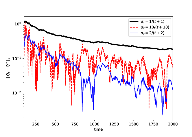
Fig. 5.1: Performance comparison with different learning rates.

5.2 Discounted problems

The LQ problem with discounting is very common in applications, in which the cost function (1.2) is usually replaced by

$$J(x,u_{\cdot})=\sum_{t=0}^{\infty}\rho^{2t}\big{[}x_{t}^{\mathsf{T}},u_{t}^{\mathsf{T}}\big{]}N_{t+1}\begin{bmatrix}x_{t}\\ u_{t}\end{bmatrix}$$

with a discounted rate $\rho>0$. With a transformation $x_{t}\mapsto\rho^{-t}x_{t}$, the discounted problem can reduced to our formulation with $\rho\varLambda_{t}$ instead of $\varLambda_{t}$, i.e.,

$$x_{t+1}=\rho\varLambda_{t+1}\begin{bmatrix}x_{t}\\ u_{t}\end{bmatrix},\quad t=0,1,2,\dots,$$ (5.2)

subject to the cost function (1.2).

Evidently, the well-posedness of the discounted problems depends on the value of the discounted rate $\rho$. Kalman [19] indicated that there is a critical point $\rho_{\max}>0$ such that the discounted problems is well-posedness if and only if $\rho<\rho_{\max}$. He also mentioned that how to determine $\rho_{\max}$ in a general problem seemed to be very difficult.

To examine the performance of Algorithm 1 around the critical point, we consider LQ problem (5.2)–(1.2) with $\varLambda_{t}$ and $N_{t}$ defined in (5.1). A direct computation gives $\rho_{\max}\approx 2.31827$ in this problem. We apply Algorithm 1 for two discounted rates, $\rho_{1}=2.25$ and $\rho_{2}=2.4$, where are very close to $\rho_{\max}$. By means of Theorem 1, the Q-learning process $Q_{t}$ converges a.s. for $\rho_{1}=2.25$ and diverges a.s. for $\rho_{2}=2.4$. Numerical simulations have well demonstrated the theoretical result (see Figure 5.2). The values closer to $\rho_{\max}$ than $\rho_{1}$ and $\rho_{2}$ may also be tested for this purpose, but when they are too near the critical point, the systematic computation errors would affect the performance substantially.

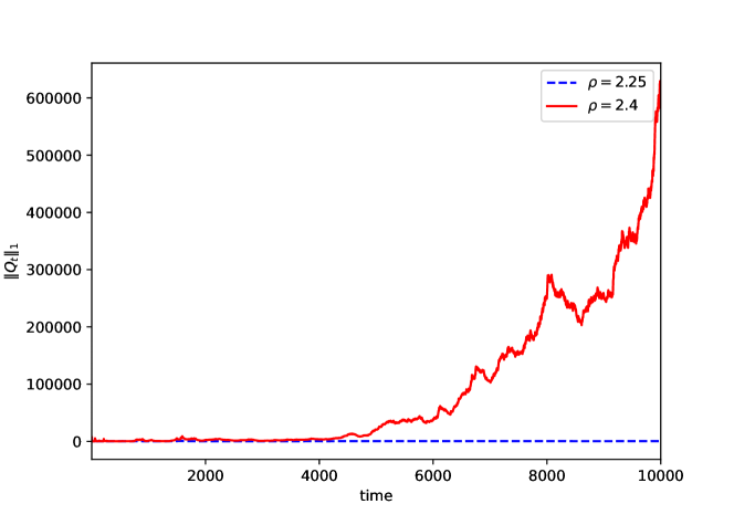
Fig. 5.2: Comparison of Q-learning processes for two discounted rates around the critical value.

5.3 Stabilization

As far as the stabilization problem is concerned, the cost function is often set as

$$J(x,u_{\cdot})=\sum_{t=0}^{\infty}|x_{t}|^{2}.$$ (5.3)

For discrete-time linear systems with random parameters, this problem was first discussed by Kalman [19]. Embedded to our framework, the parameter $N_{t}$ equals $\mathrm{diag}(I_{n},O)$ in this case, which is not positive definite. Nevertheless, in view of Remark 15, Theorem 1 can still apply if $\Phi(\mathbb{E}[N])$ is positive definite. For the system

$$x_{t+1}=A_{t+1}x_{t}+B_{t+1}u_{t},$$ (5.4)

one has that

$$\Phi(\mathbb{E}[N])=N+\mathbb{E}\begin{bmatrix}A_{t}^{\mathsf{T}}\\ B_{t}^{\mathsf{T}}\end{bmatrix}\Pi(N)[A_{t},\,B_{t}]=\begin{bmatrix}I_{n}+\mathbb{E}[A_{t}^{\mathsf{T}}A_{t}]&\mathbb{E}[A_{t}^{\mathsf{T}}B_{t}]\\ \mathbb{E}[B_{t}^{\mathsf{T}}A_{t}]&\mathbb{E}[B_{t}^{\mathsf{T}}B_{t}]\end{bmatrix}.$$

To check the condition we may need further information of the parameters.

Let us give a numerical example. Consider LQ problem (5.4)–(5.3) with $n=2$, $m=1$, and

$$A_{t} =\mathrm{e}^{w_{t}^{(1)}w_{t}^{(2)}}A^{(1)}-(\sin w_{t}^{(2)})A^{(2)}-\sqrt{w_{t}^{(2)}+w_{t}^{(3)}}A^{(3)},$$

$$B_{t} =(w_{t}^{(4)}-w_{t}^{(5)})B_{t}^{(1)}+(\cos w_{t}^{(4)})B_{t}^{(2)},$$

where $w_{t}^{(1)},\dots,w_{t}^{(5)}\sim\mathcal{U}(0,1)$ are independent, and

$$[A^{(1)},A^{(2)},A^{(3)},B^{(1)},B^{(2)}] =\rho\begin{bmatrix}-5&2&0&-1&-2&3&-1&1\\ 2&3&-4&7&6&0&1&0\end{bmatrix},$$

where $\rho$ is the discounted rate. One can check that $\Phi(\mathbb{E}[N])>O$ in this example, so Theorems 1 and (3) can apply to this problem.

We set $\rho=0.25$ with which the problem is demonstrated numerically to be well-posedness. To verify the stabilization, we conduct two control policies: the zero control $u_{t}=0$ and the adaptive feedback control $u_{t}=\Gamma(Q_{t})x_{t}$, and test three initial state $x_{0}=[1,0]^{\mathsf{T}}$, $[0,1]^{\mathsf{T}}$, and $[1,1]^{\mathsf{T}}$. Numerical simulations (see Figure 5.3) show that the system is stable under the adaptive feedback control but unstable without control (i.e., $u_{t}=0$).

$$\begin{matrix}\includegraphics[width=136.15466pt]{eg3-1}&\includegraphics[width=130.08731pt]{eg3-2}&\includegraphics[width=130.08731pt]{eg3-3}\end{matrix}$$

Fig. 5.3: Comparison of the state processes under adaptive feedback control and zero control.

References

• [1] D. L. Alspach, A dual control for linear systems with control dependent plant and measurement noise, in 1973 IEEE Conference on Decision and Control including the 12th Symposium on Adaptive Processes, IEEE, 1973, pp. 681–689.
• [2] M. Aoki, Optimization of Stochastic Systems, New York: Academic, 1967.
• [3]  , Optimal Control and System Theory in Dynamic Economic Analysis, vol. 1, North Holland, 1976.
• [4] K. J. Åström and B. Wittenmark, Adaptive control, Courier Corporation, 2013.
• [5] M. Athans, R. Ku, and S. B. Gershwin, The uncertainty threshold principle: Some fundamental limitations of optimal decision making under dynamic uncertainty, IEEE Transactions on Automatic Control, 22 (1977), pp. 491–495.
• [6] A. Beghi and D. D’Alessandro, Discrete-time optimal control with control-dependent noise and generalized riccati difference equations, Automatica, 34 (1998), pp. 1031–1034.
• [7] D. P. Bertsekas, Reinforcement learning and optimal control, Athena Scientific Belmont, MA, 2019.
• [8] H.-F. Chen and L. Guo, Optimal stochastic adaptive control with quadratic index, International Journal of Control, 43 (1986), pp. 869–881.
• [9] S.-P. Chen, X.-J. Li, and X.-Y. Zhou, Stochastic linear quadratic regulators with indefinite control weight costs, SIAM Journal on Control and Optimization, 36 (1998), pp. 1685–1702.
• [10] G. C. Chow, Analysis and Control of Dynamic Economic Systems, Wiley, 1975.
• [11] W. L. De Koning, Infinite horizon optimal control of linear discrete time systems with stochastic parameters, Automatica, 18 (1982), pp. 443–453.
• [12] R. Drenick and L. Shaw, Optimal control of linear plants with random parameters, IEEE Transactions on Automatic Control, 9 (1964), pp. 236–244.
• [13] T. E. Duncan, L. Guo, and B. Pasik-Duncan, Adaptive continuous-time linear quadratic gaussian control, IEEE Transactions on Automatic Control, 44 (1999), pp. 1653–1662.
• [14] A. Dvoretzky, On stochastic approximation, in Proceedings of the Third Berkeley Symposium on Mathematical Statistics and Probability, vol. 1, University of California Press, 1956, pp. 39–56.
• [15] M. K. S. Faradonbeh, A. Tewari, and G. Michailidis, On adaptive linear–quadratic regulators, Automatica, 117 (2020), p. 108982.
• [16] S. E. Harris, Stochastic controllability of linear discrete systems with multiplicative noise, International Journal of Control, 27 (1978), pp. 213–227.
• [17] Y. Huang, W.-H. Zhang, and H.-S. Zhang, Infinite horizon LQ optimal control for discrete-time stochastic systems, in 2006 6th World Congress on Intelligent Control and Automation, vol. 1, IEEE, 2006, pp. 252–256.
• [18] T. Jaakkola, M. I. Jordan, and S. P. Singh, Convergence of stochastic iterative dynamic programming algorithms, in Advances in Neural Information Processing Systems, 1994, pp. 703–710.
• [19] R. E. Kalman, Control of randomly varying linear dynamical systems, in Proceedings of Symposia in Applied Mathematics, 1961, pp. 287–298.
• [20] R. E. Kalman and J. E. Bertram, A unified approach to the theory of sampling systems, Journal of the Franklin Institute, 267 (1959), pp. 405–436.
• [21] R. T. Ku and M. Athans, Further results on the uncertainty threshold principle, IEEE Transactions on Automatic Control, 22 (1977), pp. 866–868.
• [22] D. N. Martin and T. L. Johnson, Stability criteria for discrete-time systems with colored multiplicative noise, in 1975 IEEE Conference on Decision and Control including the 14th Symposium on Adaptive Processes, IEEE, 1975, pp. 169–175.
• [23] T. Morozan, Stabilization of some stochastic discrete-time control systems, Stochastic Analysis and Applications, 1 (1983), pp. 89–116.
• [24] Y.-H. Ni, X. Li, and J.-F. Zhang, Indefinite mean-field stochastic linear-quadratic optimal control: from finite horizon to infinite horizon, IEEE Transactions on Automatic Control, 61 (2015), pp. 3269–3284.
• [25] L. Pronzato, C. Kulcsár, and E. Walter, An actively adaptive control policy for linear models, IEEE Transactions on Automatic Control, 41 (1996), pp. 855–858.
• [26] M. A. Rami, J. B. Moore, and X. Y. Zhou, Indefinite stochastic linear quadratic control and generalized differential Riccati equation, SIAM Journal on Control and Optimization, 40 (2002), pp. 1296–1311.
• [27] A. C. M. Ran and H. L. Trentelman, Linear quadratic problems with indefinite cost for discrete time systems, SIAM Journal on Matrix Analysis and Applications, 14 (1993), pp. 776–797.
• [28] R. S. Sutton and A. G. Barto, Reinforcement Learning: An Introduction, MIT press, 2018.
• [29] A. R. Tiedemann and W. L. De Koning, The equivalent discrete-time optimal control problem for continuous-time systems with stochastic parameters, International Journal of Control, 40 (1984), pp. 449–466.
• [30] E. Tse and Y. Bar-Shalom, An actively adaptive control for linear systems with random parameters via the dual control approach, IEEE Transactions on Automatic Control, 18 (1973), pp. 109–117.
• [31] J. N. Tsitsiklis, Asynchronous stochastic approximation and Q-learning, Machine Learning, 16 (1994), pp. 185–202.
• [32] T. Wang, H.-G. Zhang, and Y. Luo, Infinite-time stochastic linear quadratic optimal control for unknown discrete-time systems using adaptive dynamic programming approach, Neurocomputing, 171 (2016), pp. 379–386.
• [33] C. J. C. H. Watkins, Learning from delayed rewards, Ph.D. Thesis, University of Cambridge, (1989).
• [34] E. Yaz, Stabilization of deterministic and stochastic-parameter discrete systems, International Journal of Control, 42 (1985), pp. 33–41.
• [35]  , Control of randomly varying systems with prescribed degree of stability, IEEE Transactions on Automatic Control, 33 (1988), pp. 407–410.