Follow-up Observations for IceCube-170922A: Detection of Rapid Near-Infrared Variability and Intensive Monitoring of TXS 0506+056

Abstract

We present our follow-up observations to search for an electromagnetic counterpart of the IceCube high-energy neutrino, IceCube-170922A. Monitoring observations of a likely counterpart, , are also described. First, we quickly took optical and near-infrared images of 7 flat-spectrum radio sources within the IceCube error region right after the neutrino detection and found a rapid flux decline of  in Kanata/HONIR $J$-band data. Motivated by this discovery, intensive follow-up observations of   are continuously done, including our monitoring imaging observations, spectroscopic observations, and polarimetric observations in optical and near-infrared wavelengths.  shows a large amplitude ($\sim 1.0$ mag) variability in a time scale of several days or longer, although no significant variability is detected in a time scale of a day or shorter.  also shows a bluer-when-brighter trend in optical and near-infrared wavelengths. Structure functions of variabilities are examined and indicate that  is not a special blazar in terms of optical variability. Polarization measurement results of  are also discussed.

1 Introduction

Recent detections of high-energy, TeV-PeV, neutrinos realized by the IceCube experiment (Aartsen et al., 2014) have made more exciting electromagnetic identification of the neutrino sources. Such high-energy neutrinos are produced by decay of charged pions which are created through cosmic-ray interactions with radiation ($p\gamma$; Winter (2013)) or gas ($pp$; Murase et al. (2013)). Therefore, detection of high-energy neutrino is a smoking-gun evidence of existence of high-energy protons (cosmic rays). Observations of high-energy neutrinos provide unique information about cosmic-ray acceleration mechanisms and their acceleration sites, if their origins are identified.

In The IceCube Collaboration et al. (2015), detections of 54 neutrino events by the IceCube experiment in total are reported from the 4-year data. Arrival directions of the 54 IceCube events are consistent with being isotropic and do not show any clustering in the Galactic plane (The IceCube Collaboration et al., 2015), indicating the neutrino sources would be extragalactic (Aartsen et al., 2014). Neutrinos can travel cosmological distances without being deflected by cosmic magnetic field nor absorbed by photon field. On the other hand, contribution of high-redshift sources represents only a small fraction of the total observed flux due to the redshift dilution. Thus, the competition between the neutrino’s penetrating power and the redshift dilution makes emissions from sources at redshift of $z\sim 1-2$ dominant to the IceCube neutrino for single-neutrino (singlet) events (Kotera et al. (2010); Icecube Collaboration et al. (2017)). The IceCube collaboration started issuing real-time alerts in April 2016 (Aartsen et al., 2017c) and and the number of the neutrino detection is increasing.

Many hypotheses for the origin of the high energy neutrinos have been proposed, including blazars (Mannheim, 1995; Mücke et al., 2003; Becker et al., 2005), starburst galaxies (Loeb & Waxman, 2006; Bechtol et al., 2017), Type IIn supernovae (Murase et al., 2011; Aartsen et al., 2015), choked-jet supernovae (Razzaque et al., 2004; Senno et al., 2016), gamma-ray bursts (GRBs; Waxman & Bahcall (1997); Aartsen et al. (2017a)), tidal disruption events (TDEs; Senno et al. (2017)), active galactic nuclei (AGN) core (Eichler, 1979; Inoue et al., 2019).

These theories have been tried to be assessed observationally and some observational results set constraints on the theories as described in the this paragraph. Kadler et al. (2016) showed that a high fluence GeV blazar, PKS 1424-418, is a possible origin for one of the high-energy starting events (HESEs), HESE-35, based on the temporal and positional coincidence between the neutrino detection and the $\gamma$-ray flare of the blazar. This blazar shows broad CIV, CIII], and Mg II lines in its optical spectrum and is classified as a flat-spectrum radio quasar (FSRQ) at $z=1.522$ (White et al., 1988). On the other hand, in general, there is not a good spatial correlation between the neutrino detections and Fermi $\gamma$-ray blazars, indicating that contribution of the Fermi $\gamma$-ray blazars to the diffuse neutrino flux is as small as $<27$% (Aartsen et al., 2017b). No other origin candidates have been strongly supported as a significantly contributing source to the neutrino background (Bechtol et al., 2017; Senno et al., 2016, 2017). Very recently, a radio-emitting TDE at $z=0.051$ discovered on April 1, 2019, is claimed to be an associated source to the neutrino event IceCube-191001A (Stein et al., 2020).

On 22 September 2017 at 20:54:30.43 (MJD=58018.871), the IceCube experiment detected a track event of a high-energy neutrino ($\sim 290$ TeV; IceCube Collaboration et al. (2018)), IceCube-170922A, and Kopper & Blaufuss (2017) reported it via The Gamma-ray Coordinates Network (GCN) Circular. The direction is constrained to be R.A.$=77.43^{+0.95}_{-0.65}$ and Dec.$=+5.72^{+0.50}_{-0.30}$ degrees in J2000 equinox (90% confidence region). , a BL Lac blazar within the error region, was pointed out to be a good candidate of the counterpart (Tanaka et al. (2017); see also §3.1) and observed with many telescopes over a wide wavelength range after that (IceCube Collaboration et al., 2018). During the intensive follow-up observations, the redshift of  was successfully determined to be $z=0.3365$ (Paiano et al., 2018). In addition,  was detected in high-energy $\gamma$-ray with Large Area Telescope (LAT) on the Fermi satellite (Tanaka et al. (2017); IceCube Collaboration et al. (2018)), MAGIC telescope (IceCube Collaboration et al. (2018); Ansoldi et al. (2018)), and AGILE $\gamma$-ray telescope (Lucarelli et al., 2019), independently, which strength the coincidence between  and the neutrino source.

is a blazar registered in a catalog of Texas Survey of Radio Sources (Douglas et al., 1996) and one of the highest energy $\gamma$-ray emitting blazars among blazars detected by the Energetic Gamma Ray Experiment Telescope (EGRET) $\gamma$-ray (30 MeV-30 GeV) satellite (Dingus & Bertsch, 2001). The radio-to-gamma-ray spectral energy distribution (SED; IceCube Collaboration et al. (2018)) in combination with its featureless spectra (Paiano et al. (2018); IceCube Collaboration et al. (2018)) and peak frequency of $10^{14.5\pm 0.25}$ Hz (Padovani et al., 2019) indicates that  belongs to intermediate synchrotron peaked ($10^{14}<\nu_{S}<10^{15}$ Hz) BL Lac objects (ISPs or IBLs; Padovani et al. (2018)) although Padovani et al. (2019) claim that  is a masquerading BL Lac. The bolometric luminosity $L_{\rm{bol}}$ is estimated to be a few $\times 10^{45}$ erg s^-1 (Padovani et al., 2019), which is roughly consistent with being an ISP by following the so-called blazar sequence (Fossati et al., 1998; Kubo et al., 1998; Ghisellini et al., 2017).

In SEDs of BL Lacs, non-thermal emission from a relativistic jet dominates thermal emission from an accretion disk in rest-frame UV-optical wavelengths and from a dusty torus in rest-frame near-infrared (NIR) wavelengths, as well as its host galaxy. Temporal flux (luminosity) variability of blazars is sometimes explained by a shock-in-jet model (Marscher & Gear, 1985) and useful to see a possible link between neutrino emission, probably from a relativistic jet, and electromagnetic emission activities. To assess if or not  is a special blazar and September 22, 2017 is a special timing, it is worth examining variability properties of . Blazars, in general, show large and rapid variability in optical wavelengths (Bauer et al., 2009), which could be a key to understanding relationship with neutrino emission. Although it is dependent on blazar types, intranight variability is significantly detected for several tens of percent of blazars and its duty cycles are also several tens of percent (Paliya et al. (2017); Bachev et al. (2017); Gaur et al. (2017); Rani et al. (2011)). Thus, short time scale variability is also worth being examined.

Strong polarization in optical wavelengths is one of the unique characteristics of BL Lacs (e.g., Mead et al. (1990); Falomo et al. (2014); Ikejiri et al. (2011); Itoh et al. (2016)), which supports an idea that synchrotron emission dominates optical emission of BL Lacs. Temporal changes of polarization degrees and angles have been observed for many blazars (Itoh et al., 2016; Jermak et al., 2016) and these observables are keys to understanding structure and physics in relativistic jets of blazars (Brand, 1985; Visvanathan & Wills, 1998).

The structure of this paper is as follows. In section 2, we describe our follow-up observations after the alert of the IceCube-170922A, including imaging and spectroscopic observations in the optical and near-infrared wavelengths. We describe the observational results and its discussion in section 3. The neutrino direction and  are inside the Pan-STARRS1 (PS1; Chambers et al. (2016)) footprint and outside the Sloan Digital Sky Survey (SDSS; York et al. (2000)) footprint. Cosmological parameters used in this paper are $\Omega_{M}=0.3,\Omega_{\Lambda}=0.7,H_{0}=70$ km s^-1 Mpc^-1. All the observing times are specified in UT.

2 Follow-Up Observations and Data Reduction

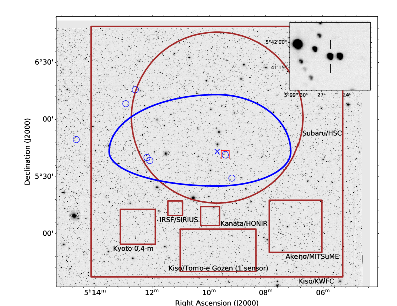
Figure 1: Coadded $r$-band image of the field taken with KWFC. North is up and east is left. The IceCube 90% containment region (IceCube Collaboration et al., 2018) is shown in blue thick ellipse and its center is indicated as a blue cross. The seven flat-spectrum radio sources in the preliminary BROS catalog which we observed first are indicated in blue small circles and  region is marked as a red rectangle, close to the blue cross. Zoom-up $1\times 1$ arcmin² view around  is also shown in the top right inset. The field-of-views of the optical and NIR instruments used in this paper are shown in brown. For Tomo-e Gozen, the field-of-view of one sensor is shown.

We started intensive follow-up observations in optical and NIR wavelengths right after receiving the realtime alert of the event. In this section, we summarize our strategy in general to identify an electromagnetic counterpart of an IceCube neutrino-emitting source (§2.1), quick observations to search for a counterpart candidate of the IceCube-170922A (§2.2), and follow-up observations after a likely counterpart, , was identified, including monitoring imaging and spectroscopic observations (§2.2,§2.3). Polarimetric observations for  are also described (§2.4).

2.1 Strategy for IceCube-170922A Electromagnetic Counterpart

Since the realtime alert system of IceCube was started in April 2016 (Aartsen et al., 2017c), we have organized a strategic optical and NIR follow-up observing group utilizing the Optical and Infrared Synergetic Telescopes for Education and Research (OISTER; Yamanaka et al. in prep.) and other Japanese facilities. Considering multiple possibilities for transient high-energy neutrino sources, we adopt multiple observing strategies using our optical and NIR facilities.

In order to test the blazar scenario, we first select blazar candidates with flat radio spectra catalogued in the BROS catalog (Itoh et al., 2020) The BROS catalog collects flat-spectrum radio sources selected using a combined catalog (de Gasperin et al., 2018) of NRAO Very Large Array Sky survey (NVSS; Condon et al. (1998); 1.4 GHz) and TIFR GMRT Sky Survey (TGSS; Intema et al. (2017); 150 MHz) catalogs. The final criterion on the radio spectral slope to select flat-spectrum objects is $\alpha>-0.6$ where $f_{\nu}\propto\nu^{\alpha}$ (Itoh et al., 2020) while the criterion was $\alpha>-0.5$ at the observation times in this paper. We carry out optical and NIR imaging observations to detect any brightness change possibly from a neutrino-emitting blazar within an IceCube localization. For this purpose, 1-2 m class telescopes in the OISTER collaboration are mainly used. A fraction of the BROS sources are apparently faint in optical and not detected in the PS1 data. We search for variabilities of such faint blazar candidates with Hyper Suprime-Cam (HSC; Miyazaki et al. (2012)) on the 8.2-m Subaru telescope.

A supernova is also thought to be one of the candidates to generate high-energy neutrinos. To find a supernova which neutrino may originate from, we also carry out wide-field imaging surveys in optical to cover a significant fraction of IceCube localization using wide-field optical imagers such as Kiso Wide Field Camera (KWFC; Sako et al. (2012)) and Tomo-e Gozen (Sako et al., 2016, 2018) on the 1.05-m Kiso Schimidt telescope and HSC on the 8.2-m Subaru telescope.

For the IceCube-170922A event, we performed optical and NIR observations with both the strategies. Our blind survey for supernovae is described in a separate paper (Morokuma et al., in prep.).

2.2 Optical and NIR Imaging

All the imaging observations are summarized below and in Table 2.2.2. Detailed characteristics of the telescopes and instruments are summarized in the table.

2.2.1 Initial Response to the Alert: Search for a rapidly variable blazar

We started follow-up imaging observations $0.8$ days after the alert of IceCube-170922A Hiroshima Optical and Near-Infrared camera (HONIR; Akitaya et al. (2014)) on the 1.5-m Kanata telescope at the Higashi Hiroshima Observatory ($R_{C}$ and $J$-bands) and KWFC on the 1.05-m Kiso Schmidt telescope ($g,r$ and $i$-bands). In subsequent nights, HSC on the 8.2-m Subaru telescope ($z$-band) and 0.5-m MITSuME Akeno telescope (Yatsu et al. (2007); Shimokawabe et al. (2008); Kotani et al. (2005); $g,R_{C}$, and $I_{C}$-bands) were also used. Field-of-views of KWFC and HSC are well suited for effectively covering the localization area given by IceCube as shown in Figure 1.

Brightness of a counterpart was unknown and difficult to predict because of unknown nature of a counterpart and unknown distance to a counterpart. Then, we adopt multiple exposure times to be 3-180 seconds as summarized in Table 2.2.2.

There were 7 flat-spectrum radio sources in a preliminary version of the BROS catalog within or right outside the 90% localization of IceCube-170922A as shown in Figure 1 and as listed in Table 2.2.2. Five sources among the seven are detected in the optical archival PS1 DR1 data. Each of the 7 BROS sources was observed basically one by one with Kanata/HONIR and MITSuME while all the seven BROS sources were covered by two KWFC pointings and two HSC pointings. As described in §3.1, we made a quick data reduction for the data and a Kanata/HONIR difference image for  revealed that it was fading in a time scale of a day.

2.2.2 Monitoring for

After detecting a rapid NIR variability of  with Kanata/HONIR (described in § 3.1), we continued monitoring  with telescopes described in §2.2.1. In addition, we carried out $J$, $H$, and $K_{s}$-band simultaneous imaging with SIRIUS (Nagayama et al., 2003; Nagayama, 2012) on the 1.4-m Infrared Survey Facility (IRSF) and $V$-band imaging with the 0.4-m Kyoto telescope. Exposure times of the single images are 10 and 60 seconds, respectively. We also took non-filter CMOS imaging data with Tomo-e Gozen (Sako et al., 2016, 2018) on the Kiso Schmidt telescope. Two fps (consecutive 0.5-sec exposure with negligible readout time) full-frame readout mode (Sako et al., 2018) was adopted. No filters were used and the sensors of Tomo-e Gozen are sensitive in $\sim 350-900$ nm (Kojima et al., 2018).

Telescopes and Instruments Used for Follow-up Imaging Observations. Mode Telescope Aperture [m] Instrument FoV Filter $t_{\rm{exp}}$ [sec] M Kyoto 0.4 - 18 arcmin (rectangle) $V$ 60 SM MITSuME (Akeno) 0.5 - 28 arcmin (rectangle) $g,R_{C},I_{C}$ 60 SM Kiso 1.05 KWFC 2.2 deg (rectangle) $g,r,i$ 10,30,60,180 M Kiso 1.05 Tomo-e Gozen ($39.7\times 22.4$ arcmin²)$\times$4^∗ No 0.5 M IRSF 1.4 SIRIUS 7.7 arcmin (rectangle) $J,H,K_{s}$ 10 SM Kanata 1.5 HONIR 6 arcmin (diameter) $R_{C},J$ 25-95 ($R_{C}$), 10-80 ($J$) SM Subaru 8.2 HSC 1.5 deg (diameter) $z$ 3-5 In the first column, S and M denote “survey” and “monitoring”, respectively. (*) indicates that when we took Tomo-e Gozen data, the instrument was operated with the limited number (4) of the sensors before the completion of the instrument with 84 sensors in 2019.

Seven flat-spectrum radio sources observed within or right outside the IceCube 90% error region. RA Dec RA Dec sep. $f_{\rm{TGSS}}$ $f_{\rm{NVSS}}$ Name (NVSS) (NVSS) (PS1) (PS1) [arcmin] [mJy] [mJy] $r(PS1)$ note BROS J0509+0541 05:09:26.0 +05:41:35.6 05:09:26.0 +05:41:35.4 4.58 406.7 546.8 15.04 TXS 0506+056, FL8YJ0509.4+0542 J0509+0529 05:09:12.0 +05:29:22.0 05:09:12.3 +05:29:22.8 15.83 25.8 17.9 17.05 No objects in latest BROS BROS J0512+0538 05:12:05.7 +05:38:41.7 05:12:05.7 +05:38:41.2 35.72 57.9 24.0 15.95 None BROS J0512+0540 05:12:11.6 +05:40:15.2 05:12:11.6 +05:40:15.6 37.03 160.9 63.0 22.62 None J0512+0615 05:12:36.0 +06:15:45.0 05:12:36.6 +06:15:43.8 54.03 24.7 10.2 20.86 No objects in latest BROS BROS J0512+0608 05:12:56.7 +06:08:19.1 05:12:56.8 +06:08:17.6 54.28 350.9 159.5 18.46 None BROS J0514+0549 05:14:40.1 +05:49:23.2 05:14:39.5 +05:49:20.3 74.11 267.6 268.0 19.87 None These are registered in the preliminary version of the BROS catalog when we started the follow-up observations. Coordinates of the sources in the NVSS and PS1 catalogs, separation from the IceCube detection center in arcmin unit, radio fluxes in 150 MHz (TGSS) and 1.4 GHz (NVSS) in mJy unit, PS1 $r$-band Kron magnitude, and some notes are listed.

Telescopes and Instruments Used for Follow-up Spectroscopic Observations. Telescope Aperture [m] Instrument Grism Filter $\lambda$ [Å] $R$ $t_{\rm{exp}}$ [sec] Date (UT) MJD Nayuta 2.0 MALLS 150 l/mm WG320 4700–8600 $600$ $900\times 6$ 2017-09-29 58025.7 Kanata 1.5 HOWPol grism NONE 4700–9200 $400$ $900\times 3$ 2017-09-29 58025.7 Subaru 8.2 FOCAS 300B SY47 4600–8200 $400$ $100\times 11$ 2017-09-30 58026.6 Subaru 8.2 FOCAS VPH850 SO58 7500–10500 $1200$ $100\times 7$ 2017-10-01 58027.6 Gemini-North 8.2 GMOS B1200 NONE 3400–4960 $3700$ $600\times(3+8)+240\times 1$ 2017-11-11,15 58071.5 $\lambda$ indicates usable wavelength ranges rather than observed wavelength ranges. $R$ indicates spectral resolutions.

2.2.3 Data Reduction of Imaging Data

All the data are reduced in a standard manner, including bias, overscan, and dark current subtractions if necessary and possible, flat-fielding, astrometry with Optimistic Pattern Matching (OPM; Tabur (2007)) or Astrometry.net (Lang et al., 2010) although some differences exist; e.g., distortion correction is applied only for HSC data. Details of the data reductions are described in Morokuma et al. (2014) for KWFC, in Tachibana et al. (2018) for MITSuME. The HSC data are analyzed with hscPipe v4.0.5, which is a standard reduction pipeline of HSC (Bosch et al., 2017). Tomo-e Gozen CMOS sensor data are also reduced with a dedicated pipeline described in Ohsawa et al. (2016).

To see intranight variability of objects, we measured apparent magnitudes of  and neighboring stars in individual frames. With these photometry results, we obtain daily-averaged magnitudes to obtain daily light curves of  and neighboring stars.

Photometry was done with SExtractor (Bertin & Arnouts, 1996) and MAG_AUTO is used. All magnitudes in optical and NIR wavelengths are measured in AB system. Optical magnitudes are calibrated relative to the PS1 Data Release 2 (DR2) catalog (Magnier et al. (2016); Flewelling et al. (2016)). Johnson-Cousins filter data are also calibrated to PS1 data in filters whose bandpasses are similar (i.e., PS1 $r$ for $R_{C}$ and PS1 $i$ for $I_{C}$). No filter Tomo-e Gozen data are also calibrated relative to $r$-band PS1 data. Magnitudes of field stars in NIR wavelengths are derived from the 2MASS database (Skrutskie et al., 2006) and converted to those in the AB system by following Tokunaga & Vacca (2005).

To search for a counterpart (§2.2.1), we apply an image subtraction method (Alard & Lupton (1998); Alard (2000)) for the imaging data with reference images of PS1 in optical and 2MASS in NIR, respectively. Except for Subaru/HSC, all of our optical imaging data are shallower than PS1 images and the depths of the search are limited by the depths of our data. On the other hand, in NIR, 2MASS data are not so deep and we also performed another subtraction in which our first (reference) images are subtracted from our new data.

For photometry for the normal images without image subtractions, we add addtional 3% errors to the errors measured with SExtractor. This is because photometry errors based on photon statistics usually underestimate the errors which should follow Gaussian distribution around the real values for non-variable objects, for example, due to imperfect flat-fielding procedure.

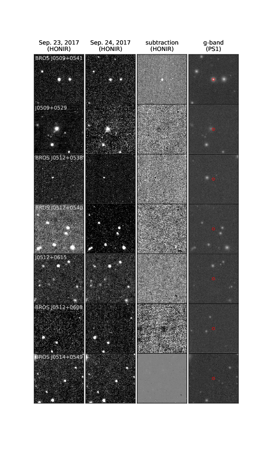
Figure 2: HONIR $J$-band images and subtracted images for the seven flat-spectrum radio sources catalogued in the preliminary BROS when we started the follow-up observations (Table 2.2.2). From left to right, HONIR $J$-band image on Sep. 23, 2017, HONIR $J$-band image on Sep. 24, 2017, subtracted HONIR $J$-band image (Sep. 23 - Sep. 24), and PS1 $r$-band image are shown for each BROS source. Red circles on the PS1 images are NVSS radio locations with radii of 2 arcsec, which are typical positional errors of NVSS sources.

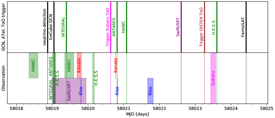
Figure 3: Timeline of the follow-up observations from the IceCube alert. Kanata/HONIR, Kiso/KWFC, and Subaru/HSC observations were shown in red, blue, and magenta, respectively. The IceCube neutrino detection, its alert, and the first Fermi/LAT GCN indicating  is a possible counterpart by (Tanaka et al., 2017) are indicated in solid black at the top panel.

2.2.4 ASAS-SN monitoring data

ASAS-SN is covering a large fraction of the sky. Long-term data nicely covering before and after the neutrino detection are available and significant variablity and brightening of  before the neutrino detection were reported in Franckowiak et al. (2017). Original ASAS-SN $V$-band data are available and taken from ASAS-SN Sky Patrol (Shappee et al. (2014); Kochanek et al. (2017)). The data are calibrated relative to AAVSO Photometric All-Sky Survey (APASS; Henden & Munari (2014)). As mentioned in IceCube Collaboration et al. (2018), the nearby west star ($g_{\rm{MeanPSF}}=14.7782\pm 0.0024$, $r_{\rm{MeanPSF}}=14.4373\pm 0.0010$, in the PS1 DR2 catalog, corresponding to $V=14.587$, which is converted using an equation in Kostov & Bonev (2018)) flux contaminates into the target flux in photometry of ASAS-SN Sky Patrol because of the coarse spatial sampling (8 arcsec pixel^-1) and large PSF ($\sim 15$ arcsec FWHM) of ASAS-SN. We estimate the contribution to the  to be 30% of the nearby star flux by calculating the contaminating flux of the nearby star into the aperture of  with the PSF size, shape (circular), and aperture adopted for the ASAS-SN photometry and subtract it from the target flux to extract only the flux of . We here do not add additional errors to the original error of . We also confirm this correction does not change our conclusions. The brightness of the nearby west star is confirmed to be almost constant over our observing period based on our data.

2.3 Optical Spectroscopy

An obstacle to study the neutrino source in detail was uncertain redshift determination of . Redshift determination of BL Lac objects is in general difficult and require a large amount of observing time with a large aperture optical telescope (Landoni et al. (2015b); Landoni et al. (2015a)) even if their images can be easily taken with 1m-class telescopes. This was the case for  and the redshift had not been reliably determined (Halpern et al., 2003).

was spectroscopically observed in the optical wavelength and the redshift is reported to be $z=0.336$ in Ajello et al. (2014). However, the origin of this redshift determination is unclear from the figure and text in the paper. MAGIC high-energy $\gamma$-ray detection (Mirzoyan (2017); Mirzoyan (2018)) gives another constraint on the redshift through the measurement of $\gamma$-$\gamma$ attenuation effect. In IceCube Collaboration et al. (2018), several conservative estimates are done with the MAGIC data and $95$% confidence level upper limit on the source redshift is $z<0.98$ while the lowest upper-limit redshift is $z<0.41$. Since there were still debates on the redshift determination before Paiano et al. (2018) determined the redsfhit to be $z=0.3365$, spectroscopic measurement was still important (Steele (2017); Morokuma et al. (2017)).

We took optical long-slit spectra with Medium And Low-dispersion Long-slit Spectrograph (MALLS) on the 2-m Nayuta telescope, HONIR (Akitaya et al., 2014) on the 1.5-m Kanata telescope, Faint Object Camera and Spectrograph (FOCAS; Kashikawa et al. (2002)) on the 8.2-m Subaru telescope, and Gemini Multi-Object Spectrograph (GMOS; Hook et al. (2004)) on the 8.2-m Gemini-North telescope. The spectral resolutions of the observations are mostly as low as $R\sim 1000$ or even lower. The exposure times are not so long, 1.5 hours at longest. These are summarized in Table 2.2.2. The FOCAS observations and spectra are described and shown in the supplement part of IceCube Collaboration et al. (2018).

All the spectra are reduced in a standard manner with IRAF, including bias subtraction, flat-fielding, wavelength calibration, sky subtraction, and source extraction, while the Gemini-N/GMOS data is reduced with the Gemini IRAF package. Wavelength calibration was done using lamp spectra or night sky lines. Flux calibration is not applied and the obtained 1d spectra are normalized with continua to see any weak emission and absorption lines.

2.4 Optical and NIR Polarimetry

We also conducted optical and NIR polarimetry observations with HONIR (Akitaya et al., 2014) at the Cassegrain focus on the 1.5-m Kanata telescope. HONIR is equipped with a rotatable half-wave plate and a Wollaston prism which enables us to conduct simultaneous polarimetry observations in an optical and an NIR channels. We used $R_{C}$-band and $J$-band in the optical and NIR channels, respectively.

The data were taken on 15 nights, from $t=8$ days to $t=213$ days after the IceCube alert ($t=0$). Each observation consisted of a set of 4 exposures at half-wave plate position angles of $0^{\circ}.0$, $22^{\circ}.5$, $45^{\circ}.0$, and $67^{\circ}.5$.

The data were reduced following a methodology of data analysis described in Kawabata et al. (1999) to derive polarization degrees and angles. Instrumental polarization induced by the optical system within the Kanata telescope and HONIR has been confirmed to be as small as 0.1-0.2% (Akitaya et al., 2014; Itoh et al., 2017).

Data taken with a fully-polarizing filter inserted in front of HONIR are used for the correction of the wavelength-dependent origin points of the position angles (originated from the multi-layered superachromatic half-wave plate). The obtained polarization degrees are as stably high as $\gtrsim 99$% with this filter in both $R_{C}$ and $J$ bands and we do not perform the depolarization correction. A strongly polarized star, BD+64d106 (Schmidt et al., 1992), was observed to correct observed position angle in the celestial coordinate and is used to calibrate the position angles of . Galactic foreground polarization should be almost negligible ($P_{R}\lesssim 0.7$% or $P_{J}\lesssim 0.2$%) because the interstellar extinction toward  is $A_{R}=0.235$ or $A_{R}=0.077$ mag (Schlafly & Finkbeiner, 2011; Serkowski et al., 1975). These values are mostly smaller than the measured values and then we do not adopt any correction for the observed polarization.

Observing epochs are separated into two as below. The first epochs are $\sim 1.5$ months after the IceCube alert. The second epochs are around $t\sim 180$ days after the alert, when larger polarization degrees of  based on polarimetric data taken with Liverpool/RINGO are reported (Steele et al., 2018). Motivated by this report, we also took additional polarization data with Kanata/HONIR.

3 Results and Discussions

3.1 Discovery of Rapid NIR Variability of

We examined the subtracted $J$-band HONIR images (HONIR-HONIR and HONIR-2MASS) to see any rapid variability of the BROS blazars and blazar candidates. Figure 2 shows HONIR-HONIR subtraction images for the 7 sources in Table 2.2.2, which were listed in the preliminary BROS catalog at the observation time. We found that  showed a fading trend, by $\sim 0.15$ mag, from Sep. 23 to Sep. 24 in 2017 as shown in the top panels of Figure 2. In $g$-band data taken with Kiso/KWFC, about $0.15$ mag decline was also detected. For the other sources, we did not find any significant NIR variability from the 2-night HONIR data or did not detect the object, which was consistent with non-detection or faint magnitudes recorded in the PS1 optical imaging data.

This rapid brightness change of  may indicate a possible relation with the neutrino detection, motivating examining Fermi $\gamma$-ray all-sky monitoring data. One of the co-authors of this paper led this effort, found its $\gamma$-ray variability, and reported it via The Astronomer’s Telegram (ATel) (Tanaka et al., 2017). This was further followed by multi-wavelength follow-up observations all over the wavelengths (Figure 3; IceCube Collaboration et al. (2018)).

Timeline from the IceCube alert (Kopper & Blaufuss, 2017) to the first Fermi ATel report (Tanaka et al., 2017) is summarized in Figure 3. After the IceCube alert, some observational reports with monitoring and follow-up data are distributed via GCN and ATel. In summary, no possible related objects to the IceCube neutrino were mentioned in any of the reports before Tanaka et al. (2017). At the event time, no significant $\gamma$-ray (INTEGRAL SPI-ACS in Savchenko et al. (2017); HAWC in Martinez & Taboada (2017); H.E.S.S. in de Naurois & H. E. S. S. Collaboration (2017)), no significant neutrino (ANTARES in Dornic & Coleiro (2017a, b)), were detected. In Swift/XRT follow-up observations, nine sources were detected (including 8 known sources) (Keivani et al., 2017) although no special notices were made for .

Optical long-term data in this field had been taken in the ASAS-SN project since October, 2012. After the report by Tanaka et al. (2017),  was reported by (Franckowiak et al., 2017) to be at the brightest phase in the ASAS-SN data and to show a brightening of $\sim 0.5$ mag in $V$-band over the last 50 days.

3.2 Light Curves of

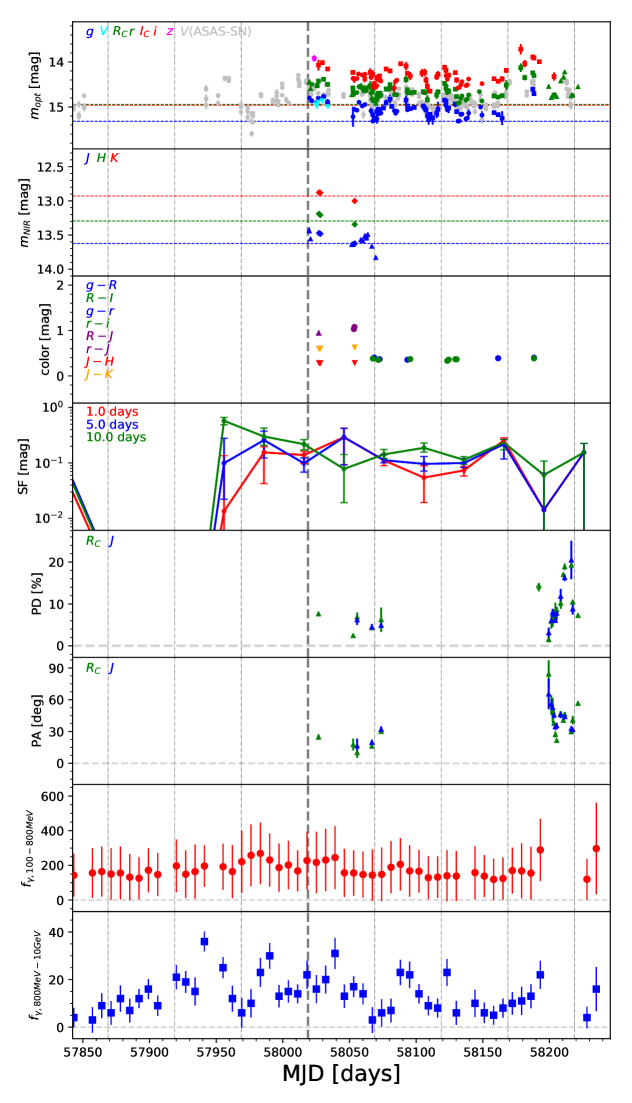
Figure 4: Daily variabilities of optical ($g$; blue, $V$: cyan, $V$ by ASAS-SN: gray, $R_{C}$ and $r$: green, $I_{C}$ and $i$: red, $z$: magenta) and NIR ($J$: blue, $H$: green, $K_{s}$: red) fluxes, optical-NIR colors from the top to the 3rd panel. Changes of the structure functions in time scales of 1.0, 5.0, and 10.0 days are shown in the 4th panel. Daily changes of polarization degree ($R_{C}$: green, $J$: blue), polarization angle ($R_{C}$: green, $J$: blue), Fermi/LAT $\gamma$-ray fluxes in 200-800 MeV and 800 MeV-10 GeV energy bands are shown from the 5th to the bottom panel. In the polarization degree, Liverpool/RINGO3 data is plotted in open circles (MJD$\sim 58192$). The neutrino detection time is indicated as gray dashed vertical lines. Vertical dash-dot gray lines indicate $-150,-100,-50,+50,+100,+150,+200$ days with respect to the IceCube neutrino detection. Galactic extinction is not corrected.

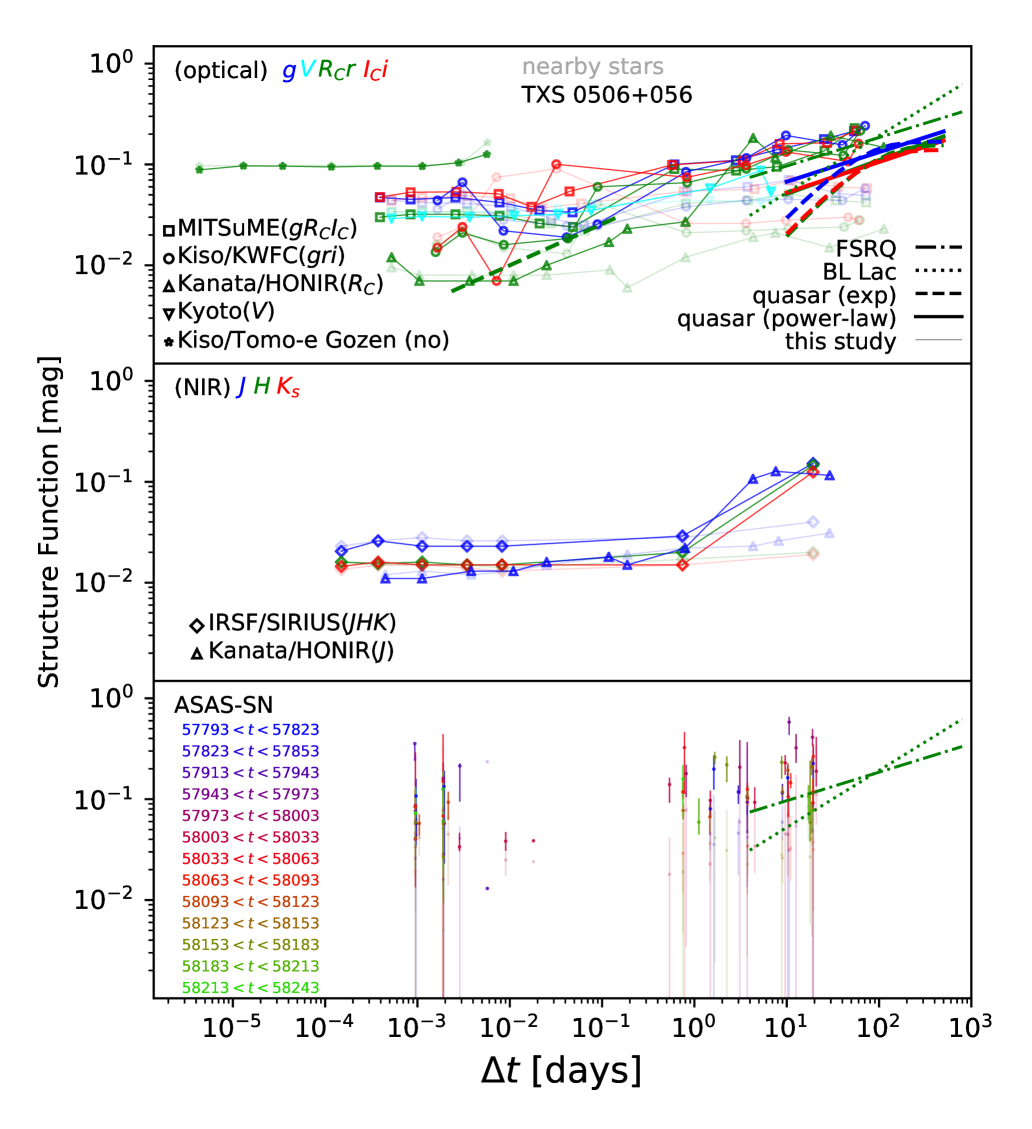
Figure 5: Optical (top) and NIR (middle) structure functions of  obtained in our observations in thick points and lines. SFs of the neighboring stars are also shown in thin points and lines to see how large the SF measurement errors are. obtained in our observations in thick points and lines. Power-law and exponential fitting results for quasars (Vanden Berk et al., 2004) are shown in blue ($g$), green ($r$), and red ($i$) thick solid and dashed lines in $\Delta{t}>10^{1}$ days, respectively. Power-law fitting results for FSRQs and BL Lacs (Bauer et al., 2009) are also shown in green dotted-dashed and dotted lines, respectively. Flat parts in short time scales are dominated by measurement errors and real SF amplitudes are thought to be lower than these lines. Optical ASAS-SN structure function as a function of period (every 30 days) is also shown in the bottom panel.

Time variabilities of the observables are shown in Figure 4, including those of optical magnitudes, NIR magnitudes, optical and NIR colors, optical and NIR polarization degrees and angles, and $\gamma$-ray fluxes in the low (100-800 MeV) and high (800 MeV-10 GeV) energy bands. In addition to our own data (§2.2), optical $V$-band data from ASAS-SN (see §2.2.4), RINGO3 optical polarimetry data (see 2.4), and Fermi $\gamma$-ray data are also used.

The $\gamma$-ray fluxes are taken from the Fermi All-sky Variability Analysis (FAVA; Abdollahi et al. (2017)) website. Aperture photometry fluxes in the low (100-800 MeV) and high (800 MeV-30 GeV) energy bands are used in this paper. We understand that the FAVA light curves are preliminary as described on the FAVA website but the temporal behavior is similar to those shown in IceCube Collaboration et al. (2018) and the FAVA data are good enough for our purpose.

3.3 Variability of

We investigate optical and NIR variabilities in three time scales including daily (§3.3.1), intranight (§3.3.2), and second-scale (§3.3.3) ones. We construct structure functions (SFs) of optical and NIR variability of , which is, in general, defined to be an ensemble variability of an object or a specific set of objects, to quantify its time variability. We compare SFs of  with those of other AGN in the literature. A caveat and problem are pointed out in Emmanoulopoulos et al. (2010) when an SF is used for studying a time scale of blazar variability, however, in this paper, we discuss only the variability amplitudes at given time scales, not the time scale itself.

We adopt an usual concept on a definition of the structure function (SF) $V(\Delta{t})$ as below,

$$V(\Delta{t}) = \sqrt{<|\Delta{m}|^{2}>-<\sigma^{2}_{S/N}>}$$ (1)

where $\Delta{t}$ is a time interval between observations, and $\Delta{m}$ is a magnitude difference between different observations and $\sigma_{\rm{S/N}}$ is measurement errors in magnitude unit. We calculate the SFs for  and neighboring stars with similar brightness to . These two SFs are compared to see any significant flux variability of . We estimate median and $1\sigma$ confidence level with a bootstrap method.

The ASAS-SN data are useful for evaluating variability behavior before and around the alert while our own data enable us to investigate short time scale variabilities after the alert.

Obtained SFs of  are shown in thick points and lines in Figure 5. SFs of the neighboring stars are also shown in thin faint points and lines in Figure 5. The SFs of are compared with those of blazars (BL Lacs and FSRQs) studied in the Palomar-QUEST survey (Bauer et al., 2009), SDSS quasars (Vanden Berk et al., 2004), and CTA102 (Bachev et al., 2017). In Bauer et al. (2009), 94 BL Lacs, 278 FSRQs, and 4 marginally classified (BL Lacs or FSRQs) objects in total are observed with 48-inch Samuel Oschin Schmidt Telescope and QUEST2 Large Area Camera ($4.6^{\circ}\times 3.6^{\circ}$ field-of-view; Baltay et al. (2007)) over 3.5 years to construct the rest-frame SFs of them as shown in Figure 5. In Vanden Berk et al. (2004), $>25,000$ quasars are observed in the 5 optical bands ($ugriz$) and rest-frame (both in time scales and wavelengths) SFs are derived. These two SFs are derived with different formulations but quantitatively equivalent with each other.

3.3.1 Long-Term Variability

Daily or longer time scale variability is summarized in this subsection. First, optical and NIR fluxes are significantly variable as shown in Figure 4. The peak-to-peak amplitude reaches up to 1 mag. We also see some fluctuations in a time scale of a few days. In addition, optical or NIR fluxes are not at their peaks at the neutrino detection as well as in $\gamma$-ray (IceCube Collaboration et al., 2018). The overall trend around the neutrino detection indicates that  is in a declining phase. About 180 days after the neutrino detection, optical and NIR brightness increase again up to a brighter level than that around the neutrino detection, however, no neutrino detection is not reported in this period.

The optical SF amplitudes of  are comparable with or slightly larger than those of AGN in the previous studies in time scales of $\Delta{t}>10^{1}$ days.  is more variable by a factor of $\sim 2$ than the SDSS quasars on average (Vanden Berk et al., 2004). The SFs of  in our measurements are larger than or comparable to those of FSRQs and BL Lacs (Bauer et al., 2009) at their face values. Note that the SFs of AGN in general have 0.1 dex or larger scatter (Vanden Berk et al. (2004); Bauer et al. (2009)), which make the envelope of the distribution is overlapped between those of FSRQs and BL Lacs and our measurements.

For NIR variability,  in $J$-band in time scales from a few days to a few tens days, and $H$ and $K_{s}$-band in a time scale of a few tens days are significantly variable than neighboring stars. The NIR variabilities of  are as large as optical ones in these time scales. NIR variabilities in shorter time scales than a few days are comparable to those of neighboring stars and are almost at the limit of the measurement errors. Typical NIR variabilities of blazars in the literature are $\sim 0.1$ mag (Sandrinelli et al. (2014); Li et al. (2018)), which is comparable to our measurement for  and this variability behavior of  is not special.

We also calculated SFs using the ASAS-SN $V$-band data in each 30 days from MJD=57793 (225 days before the neutrino detection) to MJD=58243 (225 days after the neutrino detection), covering the IceCube neutrino detection time on MJD$\sim 58018.87$. Variability amplitudes in three time scales (1, 5, and 10 days) are derived from the SFs and shown in the 4th panel of Figure 4. As a whole, there are no special periods when significantly larger variability is detected than other periods. It is not clear but the SFs marginally indicates that long-term (10 days) variability around $\sim 60$ days before the neutrino detection is the largest and larger than that in the neutrino detection period with significance of $2.1\sigma$. On the other hand, the short-term (1 day) variabilities are constant in time. This might indicate the neutrino emission would be related to the 10-days-timescale variability in this epoch. The hard $\gamma$-ray fluxes are also highly variable around this epoch (Figure 4).

Correlation between the hard $\gamma$-ray fluxes (800 MeV-10 GeV) and optical brightness is investigated as seen in Figure 6. Optical magnitudes (brightness) are negatively (positively) correlated with the $\gamma$-ray fluxes with Spearman rank correlation coefficients of $-0.471$ and $p$-values of $<0.03$. This indicates that the correlation is significant and  is brighter in optical in brighter $\gamma$-ray phases, which is consistent with general trend of ISPs or all types of blazars (Itoh et al., 2016; Jermak et al., 2016).

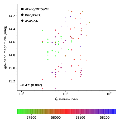
Figure 6: $g$ or $V$-band magnitude as a function of $\gamma$-ray flux. Colors of the points indicate observing epochs (MJD) as shown in the color bar.

3.3.2 Intranight Variability

During 22 nights, we contiguously took imaging data of  for a few tens minutes or longer with the 0.4-m Kyoto University telescope, MITSuME, Kanata/HONIR, and IRSF/SIRIUS. With these datasets, intranight variability can be investigated.

Magnified views of the light curves on these densely observed nights are shown in the 1st (optical) and 3rd (NIR) rows of Figure 7. In this figure, photometry is done for each frame. For a comparison, ensemble relative light curves of nearby stars with similar brightness on average are also shown in the 2nd (optical) and 4th (NIR) rows of the figure. As seen in the daily light curves in Figure 4, brightness change from night to night is easily seen. R.m.s. of the brightness is also shown in the figure.

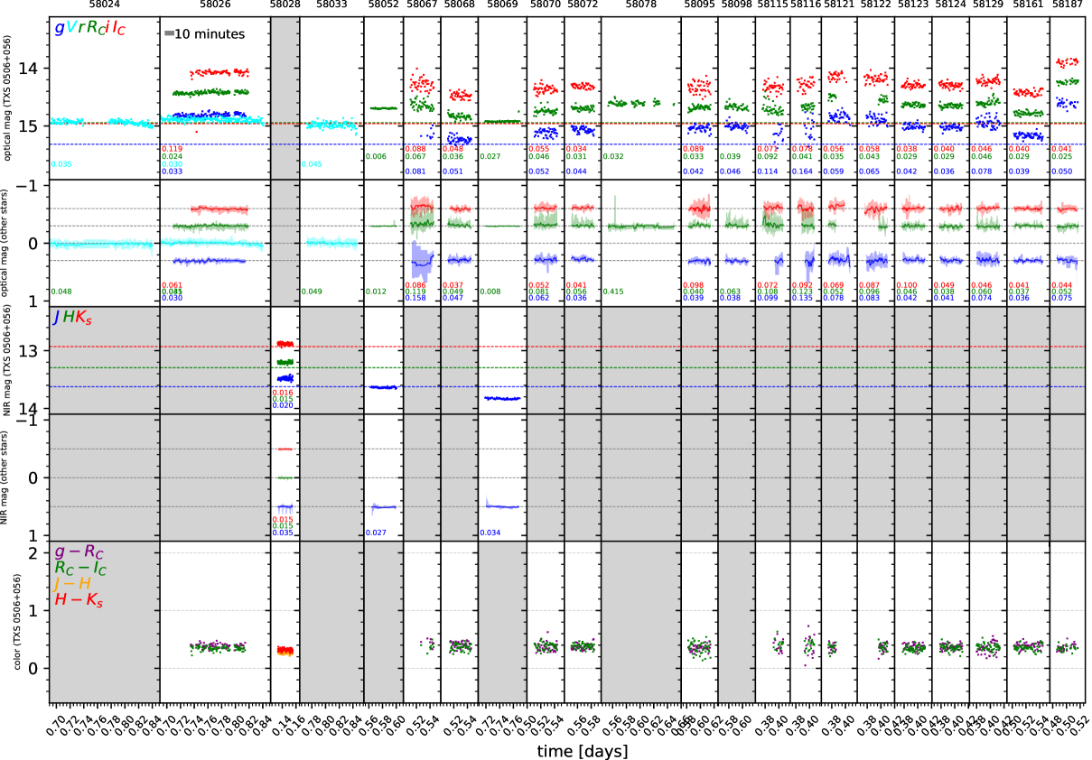
Figure 7: Light curves of  based on photometry for each frame. From top to bottom, optical light curves of , optical light curves of nearby similarly bright stars, NIR light curves of , NIR light curves of nearby similarly bright stars, and optical and optical-NIR colors of  are shown. Dates in MJD for the data are shown at the top part in each column. Colors used for the optical photometry are blue for $g$, cyan for $V$, green for $R_{C}$ and $r$, and red for $I_{C}$ and $i$. Colors used for the NIR photometry are blue for $J$, green for $H$, and red for $K_{s}$. Standard deviations in magnitude unit within a time window are shown at the left-bottom part of the panels. Optical PS1 photometry in $gri$-bands and NIR 2MASS photometry in $JHK_{s}$-bands are shown in dashed lines. A thick gray line in the top second panel shows the length of 10 minutes. Panels with no data are hatched in gray. Large scatters ($\gtrsim 0.05$ mag) are partly attributed to bad seeing.

Observed intranight variabilities are as small as $0.03-0.11$ mag, depending on the filters and epochs (the data quality) and no significant intranight variabilities are detected in our dataset. The large scatters ($\gtrsim 0.05$ mag) seen in some panels of the figure are partly attributed to bad seeing. In Sagar et al. (2004), a few to 10 percent amplitude ($\lesssim 0.1$ mag, $14.1$% at maximum) intranight $R_{C}$-band variability are seen for 11 blazars (6 BL Lacs and 5 radio core-dominated quasars). Typical observation duration in a night in Sagar et al. (2004) is 6.5 hours and the total number of the observed nights is 47. They find that a duty cycle of intranight optical variability is $\sim 60$% for BL Lacs. Similarly, Paliya et al. (2017) also monitored 17 blazars for $137$ hours in $R_{C}$-band and also obtained a high duty cycle of $\sim 40$% for blazars. Compared with these studies, the total duration (sum) of our observations shown in Figure 7 is $\sim 18$ hours and much shorter by factor of $\sim 17$ (Sagar et al., 2004) and $\sim 8$ (Paliya et al., 2017). Then, it is difficult to say any consistency of our non-detection with these two observations.

3.3.3 Second-Scale Variability

The fastest variability detected for blazars so far is a few minutes in optical (Sasada et al., 2008) and $\gamma$-ray (Albert et al., 2007; Aharonian et al., 2007; Vovk & Neronov, 2013; Vovk & Babić, 2015; Ackermann et al., 2016), which corresponds to a comparable size of a black hole, which indicates a small emitting region in a relativistic jet. A mass of a black hole hosting a blazar is expected to be as massive as $\sim 10^{9}$ M_⊙ in general (Castignani et al., 2013), and the black hole mass of  is estimated to be $\sim 3\times 10^{8}$ M_⊙ (Padovani et al., 2019) by assuming the typical host galaxy luminosity of blazars (Paiano et al., 2018) and black hole mass and bulge mass relation (McLure & Dunlop, 2002). Detection of variability in a shorter time scale would put a tight constraint on the size of an emitting region with a usually assumed Doppler boosting factor. If second scale variability was detected, this might be attributed to an apparent change in viewing angle to a bent relativistic jet (Raiteri et al., 2017).

Second-scale variability is investigated with the 2 fps Tomo-e Gozen data. Four sets of 180-second (360 frames) exposure are obtained. Detection of  is sometimes marginal and we use only photometric data of signal-to-noise ratios of $>10\sigma$. As a result, the photometric data especially in the last (fourth) exposure are partly removed in our analysis and shown in Figure 8. The resultant SF is shown in the leftmost part of the top panel of Figure 5. In our dataset, no significant rapid variability in a second time scale is detected.

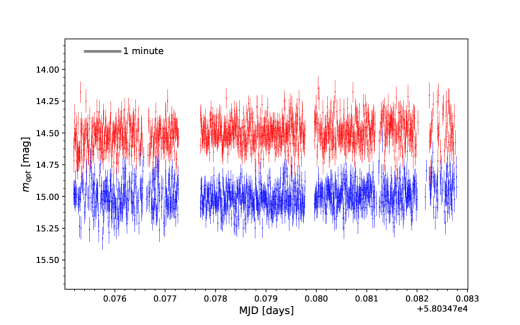
Figure 8: Optical light curves of  (red) and a nearby star (blue) taken with Tomo-e Gozen.

3.4 Optical and NIR colors of

Temporal changes of optical, optical-NIR, NIR-NIR colors are shown in Figure 4 (entire light curves), Figure 7 (intranight light curves), and Figure 9 (correlation between magnitudes and colors).

The range of the optical colors of $g-r$ and $g-R$ is 0.2-0.5 mag. A bluer-when-brighter trend is seen in the color-magnitude diagrams (Figure 9). This is consistent with an idea that   is a BL Lac-type blazar with little contribution of its accretion disk to optical-NIR emission (Bonning et al., 2012). In Figure 9, bluish data points indicating the data obtained around MJD=58200 are offset by $\sim 0.4$ mag from the most crowded (redish) data region. These bluish data also follow a tighter blue-when-brighter trend. In summary, data points in different epochs follow different color-magnitude relations. This behavior is also observed for other blazars, for example, OJ 287, and indicates different activity states between the different loci in the color-magnitude diagram in different epochs (Bonning et al., 2012). These bluish points are data taken after the $\gamma$-ray flare in March 2018 (Ojha & Valverd, 2018) while the redish points are taken after the IceCube neutrino detection (IceCube Collaboration et al., 2018). In these two epochs, increased $\gamma$-ray fluxes are detected with Fermi but the optical and NIR color-magnitude relations are different from each other. In general, the brighter locations of the bluish points at a given color may be attributed to high-energy electron injection into jet-emitting region or an emergence of much brighter accretion disk than usual possibly due to an accretion state change. Bluer-when-brighter trends of BL Lacs are sometimes attributed to a presumption that the objects are in high state (Zhang et al., 2015).  may show this trend in any state considering that almost featureless power-law continua are always observed and that the equivalent widths (EWs) of the emission lines of  (EW${}_{\rm{[OIII]}}=0.17$Å at most; Paiano et al. (2018)) are small compared to previously measured EWs of blazars (although many of these measurements are upper limits) (Landt et al., 2004).

The range of $r-J$ or $R_{C}-J$ colors of  is from 0.9 to 1.2 (Figure 9), roughly corresponding to 1.8 to 2.1 in the Vega system. The $r-J$ and $R_{C}-J$ color changes are as small as $\sim 0.3$ mag. Although the previous studies examined different colors (e.g., $V-J$ colors in Ikejiri et al. (2011)), these are typical for ISP blazars. The bluer-when-brighter trend is also seen. Note that no data points are shown in the panel of Figure 9 after the $\gamma$-ray flare in March 2018 reported by Ojha & Valverd (2018).

Intranight changes in optical colors are shown in the bottom panels of Figure 7. The $g-r$ or $g-R_{C}$ colors are almost constant, about 0.4 mag all over the nights. NIR colors of $J-H$ and $H-K_{s}$ are also almost constant in time, 0.3-0.4 mag. Note that no significant intranight variability in any band is detected (§3.3.2).

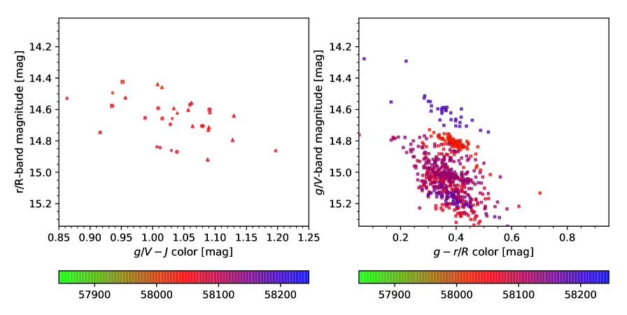
Figure 9: Optical magnitudes ($r$ or $R_{C}$ in the left panel and $g$ or $V$ in the right panel) as functions of optical-NIR color (left panel; $g-J$ or $V-J$) and optical color (right panel; $g-r$ or $g-R_{C}$). Different symbols indicate data taken with different telescopes/instruments in the same way as in Figure 4.

3.5 Polarization of

3.5.1 Temporal Changes of Polarization

Our measurement results of polarization in $R_{C}$ and $J$-bands are summarized in Table 3.5.1, including the optical polarimetric measurement taken with RINGO3 on the 2-m Liverpool telescope (Steele et al., 2018). The temporal changes of the polarization degrees and angles are shown in Figure 4.

Polarization measurements of  with Kanata/HONIR.

(*) is calculated by assuming the observations is done at UT=0 hours.

For the first 5 data points taken within 1.5 months after the alert (defined as “first epoch”), the polarization degrees are as small as 2–8% as partly reported in Yamanaka et al. (2017). About 6 months after the neutrino detection (defined as “second epoch”), Ojha & Valverd (2018) reported that a flare of the highest daily averaged $\gamma$-ray flux for  was detected with Fermi on March 13, 2018. Soon after that, Steele et al. (2018) carried out polarimetric observation on the night of March 14, 2018 with Liverpool/RINGO3 and found that optical polarization degree increases up to $\sim 14$% at wavelengths roughly corresponding to the $R_{C}$ and $I_{C}$-bands. As shown in Figure 4 and Table 3.5.1, our subsequent observations with Kanata/HONIR (12 polarization measurements for 23 days starting 8 days after the RINGO3 observation) indicate that optical polarization degree again decreases down to 1.5% on March 22, 2018, which is even lower than the observed level in the first epoch. After this decrease, the polarization degrees gradually increase up to $\sim 20$% during about two weeks and decreases again down to 7.2%, which is as low as those in the first epoch. Throughout this period, the $J$-band polarization exhibits a similar time variation behavior to that of $R_{C}$-band.

In ISPs, typical polarization degrees and their temporal change are $\sim 30$ percent and $\sim 20$ percent or less, respectively, among the samples observed by Ikejiri et al. (2011), Itoh et al. (2016), and Jermak et al. (2016). The polarization degrees and its temporal change observed in   is comparable to or less than them, being consistent with those objects.

The polarization angles are roughly constant at $\sim 20^{\circ}\pm 10^{\circ}$ in both $R_{C}$ and $J$-bands in first epoch. In the second epoch, our HONIR measurements indicate that the polarization angles are 20–90 deg and significantly different from those in the first epoch. Following the polarization degree increase from 1.5% to $\sim 20$%, the polarization angles first change from 84 deg to 22 deg and back to 30-60 deg. The position angles in $J$-band also show a similar behavior to $R_{C}$-band.

3.5.2 Correlations between Optical Brightness and Polarization

The top panel of Figure 10 shows a relation between the polarization degrees and optical $r$ or $R_{C}$-band magnitudes. Although optical brightness and polarization degrees look roughly coincident with each other as a whole (Figure 4), almost no correlations are seen during the rapid changes in the second epoch as indicated by bluish points in Figure 10. This is discussed later in this subsection.

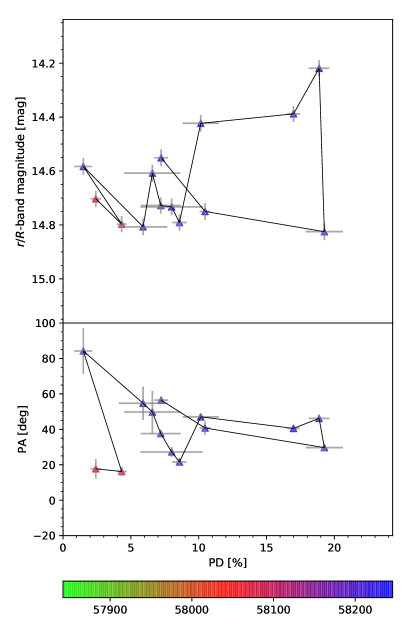
Figure 10: $r$ or $R_{C}$-band magnitude and $R_{C}$-band polarization angle as a function of $R_{C}$-band polarization degree. All the data points are connected in time sequence. Different symbols indicate data taken with different telescopes/instruments in the same way as in Figure 4.

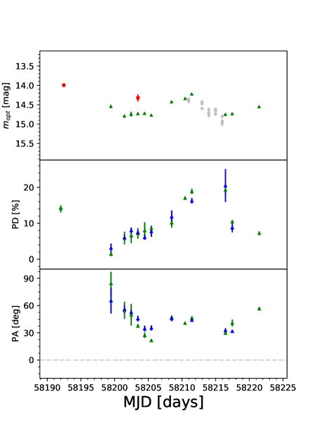
Figure 11: A magnified view of temporal changes of optical magnitudes, polarization degrees, and polarization angles around the $\gamma$-ray flare reported by Ojha & Valverd (2018). The symbols and colors are the same as those in Figure 4. $r$,$R_{C}$-band in green, $i$,$I_{C}$-band in red, and $J$-band in blue.

Polarization changes in optical wavelengths associated $\gamma$-ray flares are reported in previous literature (Sasada et al., 2008; Abdo et al., 2010). In the second epoch, the polarization change of  seems associated to the $\gamma$-ray flare (Ojha & Valverd, 2018) although such a correlated behavior is not clear in the first epoch because the polarization measurements are not done right after (or before) the neutrino detection, the measurements are sparse, and the number of the measurements is small. In Itoh et al. (2013), no brightness flare was observed during their first polarization flare for the famous blazar, CTA 102 (an FSRQ at $z=1.037$), indicating that the polarization degree does not necessarily correlate with brightness.

The lack of strong correlations between optical brightness and polarization degree in our data for  is similarly observed in previous literature for other blazars (Ikejiri et al., 2011; Jermak et al., 2016), although a significant positive correlation between “amplitudes” of flux and polarization degree is detected for two blazars (AO 0235+164 and PKS 1510-089) in 10-day time scale (Sasada et al., 2011). These observed weak correlations could be partly due to ignorance of a possible time lag between temporal changes of fluxes and polarization degrees (Uemura et al., 2017). Figure 11 is a magnified view of Figure 4 around the second epoch. The peak of polarization degrees is around MJD$\sim$58211–58217 days while that of optical brightness is around MJD$\sim$58210–58211 days. This indicates that the optical brightness change proceeds the polarization degree change, which is the opposite sense to that observed for a BL Lac, PKS 1749+096, reported by Uemura et al. (2017). This lag partly makes the correlation worse in Figure 10. A positive correlation would be seen if the data point in MJD=58216.5 (the right bottom point in Figure 10) is ignored.

The polarization angles also change in time by $\sim 70$ deg in the second epoch although the change is not so drastically large. Figure 11 indicates that the polarization angles decrease as the polarization degrees increase in the period of MJD$=58198-58207$. The polarization degrees still increase after that, however, the polarization angles do not show a systematic decrease. These make the correlation between the polarization angles and degrees poor as shown in the bottom panel of Figure 10. Changes of polarization angles are observed for many blazars (Itoh et al., 2016; Hovatta et al., 2016). The observed change of the polarization angles for  is not so large, which is sometimes explained by a curved structure of a relativistic jet (Abdo et al., 2010; Sorcia et al., 2014).

3.6 Spectra of

All of our three new spectra of  are shown in Figure 12. The Subaru/FOCAS spectra in the two different setups shown in IceCube Collaboration et al. (2018) are also plotted as references. All these spectra were taken roughly in similar epochs, $\sim 1$ week to $\sim 1.5$ months after the neutrino detection, and before the GTC/OSIRIS spectrum which conclusively determines the redshift of  was taken (Paiano et al., 2018). In the epochs of our observations,  is slightly brighter ($g=14.8-15.1$) than that in the GTC observation ($g=15.4$; Paiano et al. (2018)), which makes line detections more difficult. All of our three spectra show basically featureless continua and no significant emission or absorption lines are detected, except for the weak emission line in the Subaru/FOCAS spectrum (IceCube Collaboration et al., 2018). These are quantitatively consistent with the spectrum of Paiano et al. (2018). Any significant changes between the different epochs are not detected.

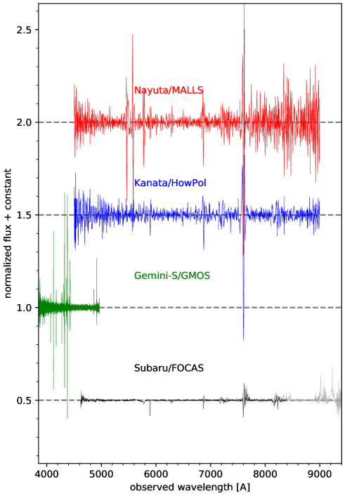
Figure 12: Optical spectra of  taken with Nayuta/MALLS (red), Kanata/HOWPol (blue), Gemini-South/GMOS (green), and Subaru/FOCAS (black and gray). The Subaru/FOCAS spectra are the same as those shown in IceCube Collaboration et al. (2018). There are no changes in spectral features. Noisy wavelength ranges are omitted. All the spiky features seen in the spectra are all atmospheric.

4 Summary

We first made optical and NIR imaging observations to search for a candidate of the neutrino source of IceCube-170922A. We found that  was rapidly fading in NIR in a day scale. Motivated by this discovery of the rapid NIR variability, the $\gamma$-ray flare was discovered in the Fermi/LAT monitoring data. We conducted monitoring observations of  with Akeno/MITSuME, Kiso/KWFC, Kiso/Tomo-e Gozen, Kyoto 0.4-m, Kanata/HONIR, and Subaru/HSC. Polarization imaging data were also taken with Kanata/HONIR at 17 epochs. We also took optical spectra four times five times with Kanata/HOWPol, Nayuta/MALLS, Gemini-N/GMOS, and Subaru/FOCAS.

Combined with ASAS-SN optical monitoring data and Fermi/LAT $\gamma$-ray data in addition to our data described above, we find

• daily variability is significant and the amplitude is as large as 1.0 mag,

• no significant intranight variability is detected,

• no special optical/NIR variability behavior over the observed period, but a very marginal sign of a larger variability in a time scale of $\sim 10$ days about 2 months before the neutrino detection,

• a weak correlation between optical/NIR and $\gamma$-ray fluxes

• large changes in polarization degrees and angles about 180 days after the neutrino detection,

• a weak or no correlation between polarization degree and optical fluxes while some correlated behavior can be seen in a part of the March 2018 ($\sim 180$ days after the neutrino detection) data,

• no significant optical spectral changes over the three months after the neutrino detection.

In summary, our data do not indicate that  is a special blazar (BL Lac) among other blazars in terms of intranight, daily, monthly optical/NIR variability, and optical polarization. The neutrino detection is also not a special timing.

For future Icecube neutrino events, to further examine possible relations between high-energy neutrinos and blazar as well as blazar variability, more complete blazar catalogs like a recently developed one, BROS (Itoh et al., 2020), are required. In addition, in optical and NIR wavelengths, routine high-cadence imaging and polarization monitoring of blazars are desired. Transient survey observations are done in several wide-field surveys such as Zwicky Transient Facility (ZTF; Graham et al. (2019)) and Tomo-e Gozen (Sako et al., 2018). Polarization monitoring is a more expensive observation program but is expected to make unique science outputs (e.g., Sakimoto et al. (2012); Itoh et al. (2016)).

We thank an anonymous referee for his/her comments to improve the manuscript. Observations with the Kanata, Nayuta, MITSuME, IRSF, and Kiso Schmidt telescopes were supported by the Optical and Near-infrared Astronomy Inter-University Cooperation Program and the Grants-in-Aid of the Ministry of Education, Science, Culture, and Sport JP23740143, JP25800103, JP16H02158, JP18H04575, JP15H02075, JP16H06341, JP18H05223, JP17K14253, JP17H04830, JP26800103, JP19H00693, JP17H06363, JP17H06362, and JP24103003.

This work was partly supported by the joint research program of the Institute for Cosmic Ray Research (ICRR). This work was also based in part on data collected at Subaru Telescope, which is operated by the National Astronomical Observatory of Japan. Based on observations obtained at the international Gemini Observatory, a program of NOIRLab, which is managed by the Association of Universities for Research in Astronomy (AURA) under a cooperative agreement with the National Science Foundation. on behalf of the Gemini Observatory partnership: the National Science Foundation (United States), National Research Council (Canada), Agencia Nacional de Investigación y Desarrollo (Chile), Ministerio de Ciencia, Tecnología e Innovación (Argentina), Ministério da Ciência, Tecnologia, Inovações e Comunicações (Brazil), and Korea Astronomy and Space Science Institute (Republic of Korea).

The IRSF project is a collaboration between Nagoya University and the SAAO supported by the Grants-in-Aid for Scientific Research on Priority Areas (A) (No. 10147207 and No. 10147214) and Optical & Near-Infrared Astronomy Inter-University Cooperation Program, from the Ministry of Education, Culture, Sports, Science and Technology (MEXT) of Japan and the National Research Foundation (NRF) of South Africa.

The Pan-STARRS1 Surveys (PS1) and the PS1 public science archive have been made possible through contributions by the Institute for Astronomy, the University of Hawaii, the Pan-STARRS Project Office, the Max-Planck Society and its participating institutes, the Max Planck Institute for Astronomy, Heidelberg and the Max Planck Institute for Extraterrestrial Physics, Garching, The Johns Hopkins University, Durham University, the University of Edinburgh, the Queen’s University Belfast, the Harvard-Smithsonian Center for Astrophysics, the Las Cumbres Observatory Global Telescope Network Incorporated, the National Central University of Taiwan, the Space Telescope Science Institute, the National Aeronautics and Space Administration under Grant No. NNX08AR22G issued through the Planetary Science Division of the NASA Science Mission Directorate, the National Science Foundation Grant No. AST-1238877, the University of Maryland, Eotvos Lorand University (ELTE), the Los Alamos National Laboratory, and the Gordon and Betty Moore Foundation.

This publication makes use of data products from the Two Micron All Sky Survey, which is a joint project of the University of Massachusetts and the Infrared Processing and Analysis Center/California Institute of Technology, funded by the National Aeronautics and Space Administration and the National Science Foundation.

The data is partly processed using the Gemini IRAF package. The authors acknowledge Dr. N. Matsunaga for a software to conduct comparisons between our image coordinates and the catalogue values.

References

- Aartsen et al. (2014) Aartsen, M. G., Ackermann, M., Adams, J., et al. 2014, Physical Review Letters, 113, 101101
- Aartsen et al. (2015) Aartsen, M. G., Abraham, K., Ackermann, M., et al. 2015, ApJ, 811, 52
- Aartsen et al. (2017a) Aartsen, M. G., Ackermann, M., Adams, J., et al. 2017a, ApJ, 843, 112
- Aartsen et al. (2017b) Aartsen, M. G., Abraham, K., Ackermann, M., et al. 2017b, ApJ, 835, 45
- Aartsen et al. (2017c) Aartsen, M. G., Ackermann, M., Adams, J., et al. 2017c, Astroparticle Physics, 92, 30
- Abdo et al. (2010) Abdo, A. A., Ackermann, M., Ajello, M., et al. 2010, Nature, 463, 919
- Abdollahi et al. (2017) Abdollahi, S., Ackermann, M., Ajello, M., et al. 2017, ApJ, 846, 34
- Ackermann et al. (2016) Ackermann, M., Anantua, R., Asano, K., et al. 2016, ApJ, 824, L20
- Aharonian et al. (2007) Aharonian, F., Akhperjanian, A. G., Bazer-Bachi, A. R., et al. 2007, ApJ, 664, L71
- Ajello et al. (2014) Ajello, M., Romani, R. W., Gasparrini, D., et al. 2014, ApJ, 780, 73
- Akitaya et al. (2014) Akitaya, H., Moritani, Y., Ui, T., et al. 2014, in Proc. SPIE, Vol. 9147, Ground-based and Airborne Instrumentation for Astronomy V, 91474O
- Alard (2000) Alard, C. 2000, A&AS, 144, 363
- Alard & Lupton (1998) Alard, C., & Lupton, R. H. 1998, ApJ, 503, 325
- Albert et al. (2007) Albert, J., Aliu, E., Anderhub, H., et al. 2007, ApJ, 669, 862
- Ansoldi et al. (2018) Ansoldi, S., Antonelli, L. A., Arcaro, C., et al. 2018, ApJ, 863, L10
- Bachev et al. (2017) Bachev, R., Popov, V., Strigachev, A., et al. 2017, MNRAS, 471, 2216
- Baltay et al. (2007) Baltay, C., Rabinowitz, D., Andrews, P., et al. 2007, PASP, 119, 1278
- Bauer et al. (2009) Bauer, A., Baltay, C., Coppi, P., et al. 2009, ApJ, 699, 1732
- Bechtol et al. (2017) Bechtol, K., Ahlers, M., Di Mauro, M., Ajello, M., & Vandenbroucke, J. 2017, ApJ, 836, 47
- Becker et al. (2005) Becker, J. K., Biermann, P. L., & Rhode, W. 2005, Astroparticle Physics, 23, 355
- Bertin & Arnouts (1996) Bertin, E., & Arnouts, S. 1996, A&AS, 117, 393
- Bonning et al. (2012) Bonning, E., Urry, C. M., Bailyn, C., et al. 2012, ApJ, 756, 13
- Bosch et al. (2017) Bosch, J., Armstrong, R., Bickerton, S., et al. 2017, ArXiv e-prints, arXiv:1705.06766
- Brand (1985) Brand, P. W. J. L. 1985, Infrared and optical photopolarimetry of blazars., ed. J. E. Dyson, 215–219
- Castignani et al. (2013) Castignani, G., Haardt, F., Lapi, A., et al. 2013, A&A, 560, A28
- Chambers et al. (2016) Chambers, K. C., Magnier, E. A., Metcalfe, N., et al. 2016, arXiv e-prints, arXiv:1612.05560
- Condon et al. (1998) Condon, J. J., Cotton, W. D., Greisen, E. W., et al. 1998, AJ, 115, 1693
- de Gasperin et al. (2018) de Gasperin, F., Intema, H. T., & Frail, D. A. 2018, MNRAS, 474, 5008
- de Naurois & H. E. S. S. Collaboration (2017) de Naurois, M., & H. E. S. S. Collaboration. 2017, The Astronomer’s Telegram, 10787, 1
- Dingus & Bertsch (2001) Dingus, B. L., & Bertsch, D. L. 2001, in American Institute of Physics Conference Series, Vol. 587, Gamma 2001: Gamma-Ray Astrophysics, ed. S. Ritz, N. Gehrels, & C. R. Shrader, 251–255
- Dornic & Coleiro (2017a) Dornic, D., & Coleiro, A. 2017a, GRB Coordinates Network, 21923, 1
- Dornic & Coleiro (2017b) —. 2017b, The Astronomer’s Telegram, 10773, 1
- Douglas et al. (1996) Douglas, J. N., Bash, F. N., Bozyan, F. A., Torrence, G. W., & Wolfe, C. 1996, AJ, 111, 1945
- Eichler (1979) Eichler, D. 1979, ApJ, 232, 106
- Emmanoulopoulos et al. (2010) Emmanoulopoulos, D., McHardy, I. M., & Uttley, P. 2010, MNRAS, 404, 931
- Falomo et al. (2014) Falomo, R., Pian, E., & Treves, A. 2014, A&A Rev., 22, 73
- Flewelling et al. (2016) Flewelling, H. A., Magnier, E. A., Chambers, K. C., et al. 2016, arXiv e-prints, arXiv:1612.05243
- Fossati et al. (1998) Fossati, G., Maraschi, L., Celotti, A., Comastri, A., & Ghisellini, G. 1998, MNRAS, 299, 433
- Franckowiak et al. (2017) Franckowiak, A., Stanek, K. Z., Kochanek, C. S., et al. 2017, The Astronomer’s Telegram, 10794, 1
- Gaur et al. (2017) Gaur, H., Gupta, A., Bachev, R., et al. 2017, Galaxies, 5, 94
- Ghisellini et al. (2017) Ghisellini, G., Righi, C., Costamante, L., & Tavecchio, F. 2017, MNRAS, 469, 255
- Graham et al. (2019) Graham, M. J., Kulkarni, S. R., Bellm, E. C., et al. 2019, PASP, 131, 078001
- Halpern et al. (2003) Halpern, J. P., Eracleous, M., & Mattox, J. R. 2003, AJ, 125, 572
- Henden & Munari (2014) Henden, A., & Munari, U. 2014, Contributions of the Astronomical Observatory Skalnate Pleso, 43, 518
- Hook et al. (2004) Hook, I. M., Jørgensen, I., Allington-Smith, J. R., et al. 2004, PASP, 116, 425
- Hovatta et al. (2016) Hovatta, T., Lindfors, E., Blinov, D., et al. 2016, A&A, 596, A78
- Icecube Collaboration et al. (2017) Icecube Collaboration, Aartsen, M. G., Ackermann, M., et al. 2017, A&A, 607, A115
- IceCube Collaboration et al. (2018) IceCube Collaboration, Aartsen, M. G., Ackermann, M., et al. 2018, Science, 361, eaat1378
- Ikejiri et al. (2011) Ikejiri, Y., Uemura, M., Sasada, M., et al. 2011, PASJ, 63, 639
- Inoue et al. (2019) Inoue, Y., Khangulyan, D., Inoue, S., & Doi, A. 2019, ApJ, 880, 40
- Intema et al. (2017) Intema, H. T., Jagannathan, P., Mooley, K. P., & Frail, D. A. 2017, A&A, 598, A78
- Itoh et al. (2020) Itoh, R., Utsumi, Y., Inoue, Y., et al. 2020, ApJ, 901, 3
- Itoh et al. (2013) Itoh, R., Fukazawa, Y., Tanaka, Y. T., et al. 2013, ApJ, 768, L24
- Itoh et al. (2016) Itoh, R., Nalewajko, K., Fukazawa, Y., et al. 2016, ApJ, 833, 77
- Itoh et al. (2017) Itoh, R., Tanaka, Y. T., Kawabata, K. S., et al. 2017, PASJ, 69, 25
- Jermak et al. (2016) Jermak, H., Steele, I. A., Lindfors, E., et al. 2016, MNRAS, 462, 4267
- Kadler et al. (2016) Kadler, M., Krauß, F., Mannheim, K., et al. 2016, Nature Physics, 12, 807
- Kashikawa et al. (2002) Kashikawa, N., Aoki, K., Asai, R., et al. 2002, PASJ, 54, 819
- Kawabata et al. (1999) Kawabata, K. S., Okazaki, A., Akitaya, H., et al. 1999, PASP, 111, 898
- Keivani et al. (2017) Keivani, A., Evans, P. A., Kennea, J. A., et al. 2017, GRB Coordinates Network, 21930, 1
- Kochanek et al. (2017) Kochanek, C. S., Shappee, B. J., Stanek, K. Z., et al. 2017, PASP, 129, 104502
- Kojima et al. (2018) Kojima, Y., Sako, S., Ohsawa, R., et al. 2018, in Society of Photo-Optical Instrumentation Engineers (SPIE) Conference Series, Vol. 10709, Proc. SPIE, 107091T
- Kopper & Blaufuss (2017) Kopper, C., & Blaufuss, E. 2017, GRB Coordinates Network, Circular Service, No. 21916, #1 (2017), 21916
- Kostov & Bonev (2018) Kostov, A., & Bonev, T. 2018, Bulgarian Astronomical Journal, 28, 3
- Kotani et al. (2005) Kotani, T., Kawai, N., Yanagisawa, K., et al. 2005, Nuovo Cimento C Geophysics Space Physics C, 28, 755
- Kotera et al. (2010) Kotera, K., Allard, D., & Olinto, A. V. 2010, JCAP, 10, 013
- Kubo et al. (1998) Kubo, H., Takahashi, T., Madejski, G., et al. 1998, ApJ, 504, 693
- Landoni et al. (2015a) Landoni, M., Falomo, R., Treves, A., Scarpa, R., & Reverte Payá, D. 2015a, AJ, 150, 181
- Landoni et al. (2015b) Landoni, M., Massaro, F., Paggi, A., et al. 2015b, AJ, 149, 163
- Landt et al. (2004) Landt, H., Padovani, P., Perlman, E. S., & Giommi, P. 2004, MNRAS, 351, 83
- Lang et al. (2010) Lang, D., Hogg, D. W., Mierle, K., Blanton, M., & Roweis, S. 2010, AJ, 139, 1782
- Li et al. (2018) Li, X.-P., Yang, H.-Y., Luo, Y.-H., et al. 2018, MNRAS, 479, 4073
- Loeb & Waxman (2006) Loeb, A., & Waxman, E. 2006, JCAP, 2006, 003
- Lucarelli et al. (2019) Lucarelli, F., Tavani, M., Piano, G., et al. 2019, ApJ, 870, 136
- Magnier et al. (2016) Magnier, E. A., Schlafly, E. F., Finkbeiner, D. P., et al. 2016, arXiv e-prints, arXiv:1612.05242
- Mannheim (1995) Mannheim, K. 1995, Astroparticle Physics, 3, 295
- Marscher & Gear (1985) Marscher, A. P., & Gear, W. K. 1985, ApJ, 298, 114
- Martinez & Taboada (2017) Martinez, I., & Taboada, I. 2017, GRB Coordinates Network, 21924, 1
- McLure & Dunlop (2002) McLure, R. J., & Dunlop, J. S. 2002, MNRAS, 331, 795
- Mead et al. (1990) Mead, A. R. G., Ballard, K. R., Brand, P. W. J. L., et al. 1990, A&AS, 83, 183
- Mirzoyan (2017) Mirzoyan, R. 2017, The Astronomer’s Telegram, 10817
- Mirzoyan (2018) —. 2018, The Astronomer’s Telegram, 12260, 1
- Miyazaki et al. (2012) Miyazaki, S., Komiyama, Y., Nakaya, H., et al. 2012, in Proc. SPIE, Vol. 8446, Ground-based and Airborne Instrumentation for Astronomy IV, 84460Z
- Morokuma et al. (2017) Morokuma, T., Tanaka, Y. T., Ohta, K., et al. 2017, The Astronomer’s Telegram, 10890
- Morokuma et al. (2014) Morokuma, T., Tominaga, N., Tanaka, M., et al. 2014, PASJ, 66, 114
- Mücke et al. (2003) Mücke, A., Protheroe, R. J., Engel, R., Rachen, J. P., & Stanev, T. 2003, Astroparticle Physics, 18, 593
- Murase et al. (2013) Murase, K., Ahlers, M., & Lacki, B. C. 2013, Phys. Rev. D, 88, 121301
- Murase et al. (2011) Murase, K., Thompson, T. A., Lacki, B. C., & Beacom, J. F. 2011, Phys. Rev. D, 84, 043003
- Nagayama (2012) Nagayama, T. 2012, African Skies, 16, 98
- Nagayama et al. (2003) Nagayama, T., Nagashima, C., Nakajima, Y., et al. 2003, in Society of Photo-Optical Instrumentation Engineers (SPIE) Conference Series, Vol. 4841, Proc. SPIE, ed. M. Iye & A. F. M. Moorwood, 459–464
- Ohsawa et al. (2016) Ohsawa, R., Sako, S., Takahashi, H., et al. 2016, in Proc. SPIE, Vol. 9913, Software and Cyberinfrastructure for Astronomy IV, 991339
- Ojha & Valverd (2018) Ojha, R., & Valverd, J. 2018, The Astronomer’s Telegram, 11419
- Padovani et al. (2018) Padovani, P., Giommi, P., Resconi, E., et al. 2018, MNRAS, 480, 192
- Padovani et al. (2019) Padovani, P., Oikonomou, F., Petropoulou, M., Giommi, P., & Resconi, E. 2019, MNRAS, 484, L104
- Paiano et al. (2018) Paiano, S., Falomo, R., Treves, A., & Scarpa, R. 2018, ApJ, 854, L32
- Paliya et al. (2017) Paliya, V. S., Stalin, C. S., Ajello, M., & Kaur, A. 2017, ApJ, 844, 32
- Raiteri et al. (2017) Raiteri, C. M., Villata, M., Acosta-Pulido, J. A., et al. 2017, Nature, 552, 374
- Rani et al. (2011) Rani, B., Gupta, A. C., Joshi, U. C., Ganesh, S., & Wiita, P. J. 2011, MNRAS, 413, 2157
- Razzaque et al. (2004) Razzaque, S., Mészáros, P., & Waxman, E. 2004, Phys. Rev. Lett., 93, 181101
- Sagar et al. (2004) Sagar, R., Stalin, C. S., Gopal-Krishna, & Wiita, P. J. 2004, MNRAS, 348, 176
- Sakimoto et al. (2012) Sakimoto, K., Akitaya, H., Yamashita, T., et al. 2012, in Proc. SPIE, Vol. 8446, Ground-based and Airborne Instrumentation for Astronomy IV, 844673
- Sako et al. (2012) Sako, S., Aoki, T., Doi, M., et al. 2012, in Proc. SPIE, Vol. 8446, Ground-based and Airborne Instrumentation for Astronomy IV, 84466L
- Sako et al. (2016) Sako, S., Osawa, R., Takahashi, H., et al. 2016, in Proc. SPIE, Vol. 9908, Ground-based and Airborne Instrumentation for Astronomy VI, 99083P
- Sako et al. (2018) Sako, S., Ohsawa, R., Takahashi, H., et al. 2018, in Society of Photo-Optical Instrumentation Engineers (SPIE) Conference Series, Vol. 10702, Ground-based and Airborne Instrumentation for Astronomy VII, 107020J
- Sandrinelli et al. (2014) Sandrinelli, A., Covino, S., & Treves, A. 2014, A&A, 562, A79
- Sasada et al. (2008) Sasada, M., Uemura, M., Arai, A., et al. 2008, PASJ, 60, L37
- Sasada et al. (2011) Sasada, M., Uemura, M., Fukazawa, Y., et al. 2011, PASJ, 63, 489
- Savchenko et al. (2017) Savchenko, V., Ferrigno, C., Ubertini, P., et al. 2017, GRB Coordinates Network, 21917, 1
- Schlafly & Finkbeiner (2011) Schlafly, E. F., & Finkbeiner, D. P. 2011, ApJ, 737, 103
- Schmidt et al. (1992) Schmidt, G. D., Elston, R., & Lupie, O. L. 1992, AJ, 104, 1563
- Senno et al. (2016) Senno, N., Murase, K., & Mészáros, P. 2016, Phys. Rev. D, 93, 083003
- Senno et al. (2017) —. 2017, ApJ, 838, 3
- Serkowski et al. (1975) Serkowski, K., Mathewson, D. S., & Ford, V. L. 1975, ApJ, 196, 261
- Shappee et al. (2014) Shappee, B. J., Prieto, J. L., Grupe, D., et al. 2014, ApJ, 788, 48
- Shimokawabe et al. (2008) Shimokawabe, T., Kawai, N., Kotani, T., et al. 2008, in American Institute of Physics Conference Series, Vol. 1000, American Institute of Physics Conference Series, ed. M. Galassi, D. Palmer, & E. Fenimore, 543–546
- Skrutskie et al. (2006) Skrutskie, M. F., Cutri, R. M., Stiening, R., et al. 2006, AJ, 131, 1163
- Sorcia et al. (2014) Sorcia, M., Benítez, E., Hiriart, D., et al. 2014, ApJ, 794, 54
- Steele (2017) Steele, I. A. 2017, The Astronomer’s Telegram, 10799
- Steele et al. (2018) Steele, I. A., Jermak, H., & Copperwheat, C. 2018, The Astronomer’s Telegram, 11430
- Stein et al. (2020) Stein, R., van Velzen, S., Kowalski, M., et al. 2020, arXiv e-prints, arXiv:2005.05340
- Tabur (2007) Tabur, V. 2007, PASA, 24, 189
- Tachibana et al. (2018) Tachibana, Y., Arimoto, M., Asano, K., et al. 2018, PASJ, 70, 92
- Tanaka et al. (2017) Tanaka, Y. T., Buson, S., & Kocevski, D. 2017, The Astronomer’s Telegram, 10791
- The IceCube Collaboration et al. (2015) The IceCube Collaboration, Aartsen, M. G., Abraham, K., et al. 2015, ArXiv e-prints, arXiv:1510.05223
- Tokunaga & Vacca (2005) Tokunaga, A. T., & Vacca, W. D. 2005, PASP, 117, 421
- Uemura et al. (2017) Uemura, M., Itoh, R., Liodakis, I., et al. 2017, PASJ, 69, 96
- Vanden Berk et al. (2004) Vanden Berk, D. E., Wilhite, B. C., Kron, R. G., et al. 2004, ApJ, 601, 692
- Visvanathan & Wills (1998) Visvanathan, N., & Wills, B. J. 1998, AJ, 116, 2119
- Vovk & Babić (2015) Vovk, I., & Babić, A. 2015, A&A, 578, A92
- Vovk & Neronov (2013) Vovk, I., & Neronov, A. 2013, ApJ, 767, 103
- Waxman & Bahcall (1997) Waxman, E., & Bahcall, J. 1997, Phys. Rev. Lett., 78, 2292
- White et al. (1988) White, G. L., Jauncey, D. L., Savage, A., et al. 1988, ApJ, 327, 561
- Winter (2013) Winter, W. 2013, Phys. Rev. D, 88, 083007
- Yamanaka et al. (2017) Yamanaka, M., Tanaka, Y. T., Mori, H., et al. 2017, The Astronomer’s Telegram, 10844
- Yatsu et al. (2007) Yatsu, Y., Kawai, N., Shimokawabe, T., et al. 2007, Physica E Low-Dimensional Systems and Nanostructures, 40, 434
- York et al. (2000) York, D. G., Adelman, J., Anderson, John E., J., et al. 2000, AJ, 120, 1579
- Zhang et al. (2015) Zhang, B.-K., Zhou, X.-S., Zhao, X.-Y., & Dai, B.-Z. 2015, Research in Astronomy and Astrophysics, 15, 1784