Scheduling of Operations in Quantum Compiler ^∗

Abstract

When scheduling quantum operations, a shorter overall execution time of the resulting schedule yields a better throughput and higher fidelity output. In this paper, we demonstrate that quantum operation scheduling can be interpreted as a special type of job-shop problem. On this basis, we provide its formulation as Constraint Programming while taking into account commutation between quantum operations. We show that this formulation improves the overall execution time of the resulting schedules in practice through experiments with a real quantum compiler and quantum circuits from two common benchmark sets.

I Introduction

Although rapid progress in quantum computing device technology has dramatically increased the coherence time of quantum bits (or qubits), the currently available quantum computers remain in the so-called noisy intermediate scale quantum regime [1]. For noisy quantum computers, it is important to schedule the operations on qubits to be as short as possible because this increases the probability of completing all of the operations before any qubit decoheres, thus obtaining computational results with higher fidelity. Even for fault-tolerant quantum computers, shortening the duration of compiled schedules would increase the throughput.

Compilers for quantum computers (or quantum compilers) take a quantum circuit, which is a sequence of quantum operations, as an input program and generate a corresponding sequence of control instructions that are executable on the target hardware. For example, in the case of quantum computers using superconducting qubits, a quantum operation is compiled into several controls (e.g., a microwave pulse) for a certain period of time. In general, any given quantum operation has its own processing time and occupies its acting qubits for the duration as a computational resource. For this reason, scheduling, through which the execution start time of each quantum operation is determined without any overlapping, is an essential task in quantum compilers. We call this task quantum operation scheduling. In this paper, we aim to minimize the overall execution time. In the context of scheduling tasks across multiple resources (qubits, in the case of quantum operation scheduling), the time between the start of the first task and the end of the final task across all resources is known as the makespan of the schedule. Schedule length, overall execution time, and makespan are used interchangeably in this work.

The rough compilation flow considering the quantum operation scheduling task independently is as follows.

1. Gate decomposition: A task decomposes unitary operations called gates with three or more qubits into those with one or two qubits.

2. Local simplification: A task simplifies a specific sequence of gates into one gate (or cancels them out).

3. Qubit routing: A task transforms a given circuit into an equivalent circuit so that all two-qubit gates are executed on limited pairs of qubits (depending on the physical implementation of the quantum computing device).

4. Quantum operation scheduling.

5. Control instruction mapping: A task maps each quantum operation to the corresponding control instructions.

Most of the previous studies on quantum compilers have handled quantum operation scheduling within the context of its before and after tasks, e.g., qubit routing and control instruction mapping  [2, 3, 4, 5]. However, in practice, decomposing an entire compilation job into independent tasks is becoming more common in the software architecture of quantum compilers, similar to that of classical compilers, e.g., [6]. Therefore, we focus on the following research question: How much can we optimize the resulting schedule in quantum operation scheduling by itself?

In this paper, we examine quantum operation scheduling (QOS) and analyze its theoretical properties and practical usefulness. Our main contributions are as follows.

• We show that QOS obtains greater degrees of freedom for optimizing the resulting schedule by further considering the commutativity of particular quantum operations (Section III-A).

• We demonstrate that QOS can be reduced to a special type of job-shop problem that has a disjunctive graph representation (Section III-C) so that we can formulate QOS as Constraint Programming and Mixed Integer Programming, which are common techniques for the job-shop problem or scheduling in general (Section IV).

• We demonstrate through experiments with two common benchmark sets that the consideration of commutativity in QOS reduces the schedule length by up to 7.36% (Section V).

II Related Work

The job-shop problem, also known as job shop scheduling, is a well known optimization problem in computer science and operations research, and many variations of it have been studied [7, 8]. See Section III-B for its definition. Algorithms to solve this problem include exact ones such as branch-and-bound based on a Mixed Integer Programming (MIP) formulation [9], heuristic ones such as shifting bottleneck [10], and meta-heuristic ones such as simulated annealing [11]. In this paper, we mainly focus on the exact algorithm, as we want to determine the effect of optimizing quantum operation scheduling (QOS).

Task scheduling, which is the scheduling of computational tasks on multiple classical processors, has been extensively studied [12, 13]. A special type of task scheduling, Directed Acyclic Graph (DAG) scheduling, which deals with heterogeneous processors [14, 15], is most similar to QOS, but it differs in the way that resource constraints are handled. In DAG scheduling, every task can be executed on any processor with a different cost, i.e., the resource constraint is soft, while in quantum operation scheduling, every quantum operation has fixed qubit operands that are not interchangeable, i.e., the resource constraint is hard.

Qubit routing is a task that transforms a given circuit into an equivalent circuit so that all two-qubit operations in it can be executed on limited pairs of qubits. Schedule length can be approximated by circuit depth, which is the schedule length when assuming all operations have the same unit processing time. Therefore, qubit routing with the objective of minimizing the circuit depth [16, 17] or two-qubit gate depth [18, 19] can be viewed as approximate quantum operation scheduling with qubit routing. Although the algorithms for this may be applicable to scheduling without qubit routing, they provide only approximate solutions, not the exact ones to QOS.

While we define quantum operation scheduling independently of hardware technology, there are several studies on scheduling specialized for quantum computers based on ion trap technology [20, 21]. These works consider a combination of scheduling and qubit routing under a hardware structure model, called macroblocks, and propose heuristic algorithms to solve it.

Several studies have considered the commutation of quantum operations in scheduling [2, 3, 4, 5]. Venturelli et al. [2] examined the scheduling of quantum operations as a subproblem of qubit routing. They proposed an exact method using a temporal planner and showed it works well for QAOA circuits, which have many commuting gates. Although their method is applicable to quantum operation scheduling without qubit routing, our methods discussed in Section IV are simpler and perform sufficiently well for the specific scheduling problem considered in this paper. Guerreschi and Park [4] proposed a two-step solution that decomposes the problem with qubit routing and solves quantum operation scheduling (without qubit routing) in the first step. They provide a list scheduling heuristic algorithm using upward ranking but not any exact algorithm for scheduling. Other studies have considered quantum operation scheduling as a subtask of qubit routing [3] or control optimization [5]. While they provide practical heuristic algorithms for solving the task that includes scheduling, the exact algorithm for scheduling is not discussed.

III Problem

III-A Quantum Operation Scheduling

We define quantum operation scheduling as the problem of finding a schedule for a given quantum circuit. A quantum circuit is a sequence of quantum operations. Many of them are unitary operations called gates. Each of the quantum operations has acting qubits and its own processing time. A quantum circuit is given as a sequence: e.g., $[H(1),\mathit{CX}(1,2),X(2)]$. Here, $H(1)$ denotes a Hadamard gate acting on qubit $1$, $\mathit{CX}(1,2)$ denotes a Controlled-NOT (or CNOT) gate acting on control qubit $1$ and target qubit $2$, and $X(2)$ denotes a NOT gate acting on qubit $2$. Quantum circuits are typically depicted in a circuit diagram, as shown in Fig. 1.

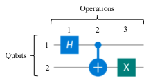
Figure 1: Diagram representation of a quantum circuit

For simplicity, we assume all of the operations have the same unit processing time in Fig. 1. If we ignore commutation between gates, the gate dependency graph is linear, i.e., $H(1)$ must precede $\mathit{CX}(1,2)$ and $\mathit{CX}(1,2)$ must precede $X(2)$, and we obtain a trivial schedule (makespan = 3), as shown in Fig. 2. We call the graph representing the dependencies among gates in a circuit the dependency graph. In contrast, if we consider that $\mathit{CX}(1,2)$ and $X(2)$ commute, we have a different dependency graph: $H(1)$ must precede $\mathit{CX}(1,2)$, but there is no restriction on $X(2)$, so we can obtain a shorter schedule (makespan = 2), as shown in Fig. 3. This is compelling evidence that commutation rules should be considered when scheduling circuit operations.

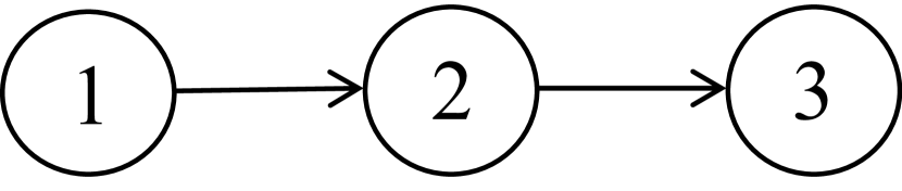
(a) Standard DAG

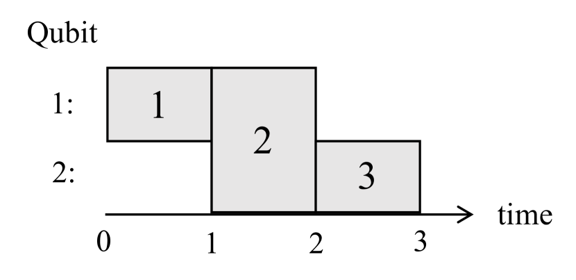
(b) Schedule with makespan = 3

Figure 2: Standard dependency graph and resulting schedule

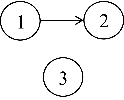
(a) Extended DAG

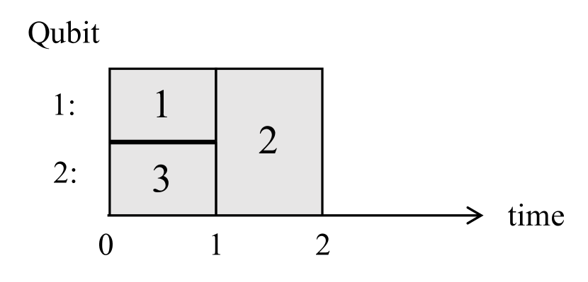
(b) Schedule with makespan = 2

Figure 3: Extended dependency graph and resulting schedule

A schedule is defined by the start times of the operations in a given circuit. Any schedule must satisfy two elementary constraints: precedence and non-overlap. The precedence constraint restricts the execution order of operations to obey a partial order represented as a dependency graph. The non-overlap constraint allows only the processing of one operation on a qubit at a time.

Generally, the supported basic operations and the processing times depend on the target hardware. Hereafter, we assume that basic operations are given and that all circuits have already been decomposed into them. We also assume that each processing time of the basic operations is fixed and given as a parameter. The dependency graph of a provided quantum circuit varies depending on which commutation rules are considered. Taking these details into account, we formally define a quantum operation scheduling problem as follows.

Quantum Operation Scheduling

Given a quantum circuit as a sequence of basic operations, each processing time of each operation, and a set of commutation rules between basic operations, find a schedule that satisfies precedence and non-overlap constraints with the minimum makespan.

III-B Job-shop Problem and its Disjunctive Graph Representation

We review a basic version of the job-shop problem as follows. Let $J=\{J_{1},\ldots,J_{n}\}$ be a set of $n$ jobs and $M=\{M_{1},\ldots,M_{m}\}$ be a set of $m$ machines. Each job $J_{j}$ has an operation sequence $O_{j}$ to be processed in a specific order, called the precedence constraint. We denote the $k$-th operation in $O_{j}$ by $O_{jk}$. Each operation $O_{jk}$ requires exclusive use of a specific machine for its processing time $p_{jk}$, called the non-overlap constraint. A schedule is a set of start (or completion) times for each operation $t_{jk}$ that satisfies both constraints. The objective of the job-shop problem is minimization of the makespan.

The job-shop problem is often represented by a disjunctive graph $G=(V,C\cup D)$, where

• $V$ is a set of nodes representing the operations $O_{jk}$,

• $C$ is a set of conjunctive (directed) edges representing the order of the operations in any job, and

• $D$ is a set of disjunctive edges representing pairs of operations that must be processed on the same machine.

For each node, the processing time and the required machine of its corresponding operation is attached. Conjunctive edges $C$ represent the precedence constraint and disjunctive edges $D$ represent the non-overlap constraint. Note that disjunctive edges whose direction is fixed by some conjunctive edges can be omitted. That means any disjunctive edge can be removed if there exists a path from one end of the edge to the other on a conjunctive graph $(V,C)$. Figure 4 shows an example of a disjunctive graph representing the job-shop problem. The operation $O_{11}$ must be processed in machine $M_{1}$ and it takes $1$ time unit. The disjunctive edge $(O_{12},O_{13})$ is omitted since its direction is fixed by the conjunctive edge at the same place.

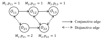
Figure 4: Disjunctive graph representation of a job-shop problem

On the basis of this disjunctive graph representation, the job-shop problem can be seen as a problem of determining the direction of disjunctive edges while keeping the resulting graph acyclic. This is equivalent to determining the ordering of the operations processed on the same machine, and such ordering yields a unique schedule, called a semi-active schedule [22], by sequencing operations as early as possible.

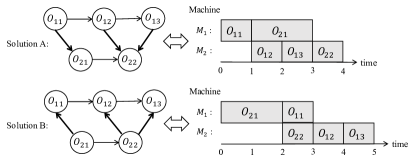
Figure 5: Two solutions to the job-shop problem in Fig. 4

Figure 5 shows two solutions to the job-shop problem defined by the disjunctive graph depicted in Fig. 4. As shown, a different selection of the direction of the disjunctive edges results in a different solution. Among the operations $\{O_{12},O_{13},O_{22}\}$, we cannot select {$(O_{22},O_{12})$, $(O_{13},O_{22})$} because it produces a cycle $O_{12}\rightarrow O_{13}\rightarrow O_{22}\rightarrow O_{12}$. In Solution A, the directed edge $(O_{11},O_{21})$ determines the order of operations processed on machine $M_{1}$, and {$(O_{12},O_{22})$, $(O_{13},O_{22})$} determine that on machine $M_{2}$.

III-C Disjunctive Graph Representation of Quantum Operation Scheduling

Technically, quantum operation scheduling can be seen as a special type of job-shop problem with the following properties: (1) one job has one operation, (2) a precedence constraint is given as a partial ordering among all operations instead of total ordering of operations per job, and (3) multiple machines (i.e., qubits) can be occupied by a single operation at the same time. Those properties preserve enough conditions to represent the problem by a disjunctive graph $G=(V,C\cup D)$. For property (1), we need to define the problem on operations without jobs, but this does not change the fact that nodes $V$ represent operations. For properties (2) and (3), we need to modify the definition of conjunctive edges $C$ and disjunctive edges $D$, respectively as follows.

The quantum operation scheduling can be represented by a disjunctive graph $G=(V,C\cup D)$, where

• $V$ is a set of nodes representing the quantum operations in a given circuit,

• $C$ is a set of conjunctive edges representing dependencies among the operations, i.e., edges of the dependency graph, and

• $D$ is a set of disjunctive edges representing pairs of operations that act on the same qubit and (possibly) commute with one another.

For each operation (i.e., node) $i\in V$, the processing time $p_{i}$ and the acting qubits are attached. Note that conjunctive graph $(V,C)$ is a DAG given as a dependency graph. Conjunctive edges $C$ and disjunctive edges $D$ still represent the precedence constraint and non-overlap constraint, respectively. It is known that the dependency graph for any circuit can be computationally constructed under several popular commutation rules [23]. When provided with the dependency graph of a quantum circuit, the disjunctive graph representation can be computationally constructed. In fact, it is possible to define disjunctive edges by all the pairs of nodes that acting on the same qubit. This definition is redundant, but there is no problem with including edges (pairs of operations) that do not commute with one another. The point is that it must include all of the commuting pairs. Starting from the redundant edges, we can define the minimal disjunctive edges by removing edges that have a path on the conjunctive graph. However, this comes at a significant computation cost. There is an in-between definition that picks up operations acting on any qubit and splits them into sets of operations commuting each other within each of the sets. We used this definition for the experiments discussed in Section V. Although this cannot provide the minimal edges because the operations within a set may not commute each other when considering operations acting on the other qubits, it has fewer edges than the most redundant definition and requires less computation cost than the minimal definition.

With the disjunctive graph representation of the quantum operation scheduling, we take the commutation of operations into account on the basis of the difference of the dependency graph. We call the dependency graph that considers only the trivial commutation between operations not sharing their acting qubits standard DAG and the dependency graph that considers commutation rules in addition to the trivial ones extended DAG.

(a) Standard DAG

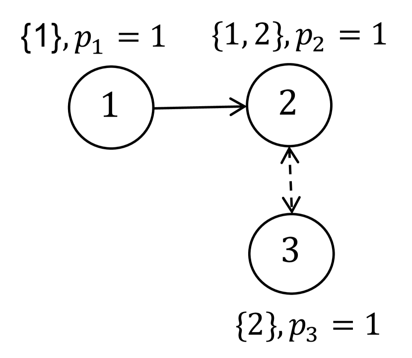
(b) Extended DAG

Figure 6: Disjunctive graphs representing quantum operation scheduling for different dependency graphs

Figure 6 shows disjunctive graphs representing two quantum operation scheduling problems that have the same operations but different dependency (conjunctive) graphs (standard DAG and extended DAG). In the case of extended DAG, we can select the order of $O_{2}$ and $O_{3}$, while in standard DAG, all the orders among operations are fixed.

It generally holds that if we consider a standard DAG, there are no disjunctive edges, i.e., $D=\emptyset$. This means there is a unique semi-active schedule because each ordering of the operations processed on the same qubit is uniquely determined by the conjunctive DAG. However, if we consider an extended DAG, we have fewer edges in $C$ and some edges in $D$. This creates the room for selecting a better ordering of the operations processed on the same qubit, i.e., optimizing the schedule.

IV Formulation

We provide a Constraint Programming (CP) formulation and a Mixed Integer Programming (MIP) formulation for the quantum operation scheduling problem (QOS) defined in the previous section. By solving them, we can find the optimal solution of QOS and analyze how much we can improve the resulting schedule in QOS. In this section, we assume that the disjunctive graph representation of quantum operation scheduling $G=(V,C\cup D)$ for a given circuit has already been constructed.

IV-A Constraint Programming Formulation

Let $x_{i}$ be an interval variable describing the start and end time of operation $i\in V$, whose duration is fixed to its processing time $p_{i}$. Using functions commonly supported by CP solvers, e.g. $\mathbf{interval\_var}$, quantum operation scheduling is formulated as a CP:

$$\begin{array}[]{ll}\mbox{minimize}&\max\{\mathbf{end\_of}(x_{i})\mid i\in V\}\\ \mbox{subject to}&\mathbf{end\_before\_start}(x_{i},x_{j}),\ \forall(i,j)\in C,\\ &\mathbf{no\_overlap}(x_{k},x_{l}),\ \forall(k,l)\in D,\\ &x_{i}\equiv\mathbf{interval\_var}(\mathrm{duration}=p_{i}),\ \forall i\in V.\\ \end{array}$$

Here $\mathbf{end\_of}(x_{i})$ takes the end time of $x_{i}$, so the objective is the minimization of the makespan. The constraint $\mathbf{end\_before\_start}(x_{i},x_{j})$ means the end time of $x_{i}$ must precede the start time $x_{j}$, so it represents the precedence constraint. The constraint $\mathbf{no\_overlap}(x_{k},x_{l})$ means the interval $x_{k}$ must not overlap the interval $x_{l}$, so it represents the non-overlap constraint. Note that, for any operation pair $(i,j)\not\in D$, the precedence constraint guarantees no overlap between them. All of $\mathbf{end\_of}$, $\mathbf{end\_before\_start}$, $\mathbf{no\_overlap}$, and $\mathbf{interval\_var}$ are supported in the IBM ILOG CP Optimizer.

IV-B Mixed Integer Programming Formulation

Let $x_{i}$ be a variable representing the start time of operation $i\in V$ and $p_{i}$ be a constant parameter representing its processing time. Let $t$ be a makespan of the schedule defined by $x$. Let $y_{kl}$ be an indicator (Boolean) variable that takes True (1) if operation $k$ precedes operation $l$ and False (0) if $l$ precedes $k$. Using these, quantum operation scheduling is formulated as a MIP:

$$\begin{array}[]{ll}\mbox{minimize}&t\\ \mbox{subject to}&x_{i}+p_{i}\leq x_{j},\ \forall(i,j)\in C,\\ &\ y_{kl}\Rightarrow x_{k}+p_{k}\leq x_{l},\ \forall(k,l)\in D,\\ &\neg y_{kl}\Rightarrow x_{l}+p_{l}\leq x_{k},\ \forall(k,l)\in D,\\ &x_{i}+p_{i}\leq t,\ \forall i\in V,\\ &0\leq x_{i}\in\mathbb{R},\ \forall i\in V,\\ &y_{kl}\in\{0,1\},\ \forall(k,l)\in D.\\ \end{array}$$

The inequality $x_{i}+p_{i}\leq x_{j}$ represents the precedence constraint. The two inequalities using $\Rightarrow$ represent the non-overlap constraint. Note that the constraints with indicator variables $y$ can be translated into linear constraints by applying the so-called the big-M technique. However, recent MIP solvers have the capability to handle such indicator constraints very well, so we leave the formulation with indicator variables.

V Experiment

We conducted two experiments. In the first one, we evaluate how much the consideration of commutation between operations improves the schedule in quantum operation scheduling. In the second one, we investigate how much the extent of improvement in scheduling can be affected by the optimization level in a previous task.

V-A Common Experimental Settings

Both of the experiments were conducted in a real compiling environment. As the target quantum computing device for compilation, we used the IBM Q Johannesburg, which has 20 qubits (see [24] for the details). We implemented our scheduling algorithms within Qiskit 0.18.0 (Terra 0.13.0), which is an open-source quantum computing software development framework [6].

We first transpiled all of the circuits to make them executable on the IBM Q Johannesburg, i.e., we solved the qubit routing problem to map given circuits onto the device topology. For this, we used the “transpile()” function in Qiskit and set the ibmq_johannesburg backend, fixed the seed_transpiler to 1, the optimization_level to 2, and left the other options as the default. During transpiling, all of the circuits were decomposed into the basis gates $\{u1,u2,u3,\mathit{CX}\}$, which are elementary gates supported by the backend. Here $u1,u2,u3$ are single-qubit gates and $\mathit{CX}$ is a two-qubit gate. The execution time for each gate (gate length) is provided as the backend properties. Note that it can differ depending on which qubit(s) the gate acts on, e.g. the length of $u3(1)$ can be different from that of $u3(2)$. We used those as of April 11, 2020.

We then applied our scheduling algorithms to the transpiled circuits. We used the real processing time for each of the basis gates provided as backend properties. We considered three commutation rules on the basis gates—$u1(i)\leftrightarrow\mathit{CX}(i,j)$, $\mathit{CX}(i,j)\leftrightarrow\mathit{CX}(i,k)$, and $\mathit{CX}(i,k)\leftrightarrow\mathit{CX}(j,k)$—in the construction of the extended DAGs for the transpiled circuits.

We used the IBM ILOG CP Optimizer and CPLEX 12.9.0 to solve the scheduling problem based on the CP and MIP formulation described in Section IV, respectively.

V-B Improvement by Considering Commutation in Quantum Operation Scheduling

In the first experiment, we quantified the significance of considering the commutation of operations in quantum operation scheduling. Specifically, we evaluated the improvement by comparing the best solutions (makespans) of the formulation constrained by standard DAG with those by extended DAG as shown in Table I.

TABLE I: Comparison of makespans [$dt$] ($1\,dt=2/9\,$ns) obtained by the formulation based on standard-DAG (Std-DAG) and those based on extended DAG (Ext-DAG) for 16 circuits from the RevLib benchmark. For the Ext-DAG formulation, the solutions by the Constraint Programming solver with the time limit of ten seconds are listed. The Qubits and Gates columns list the number of qubits and gates in the input circuits. The $\Delta$ column lists the improvement rate from Std-DAG to Ext-DAG.

Circuit name	Qubits	Gates	Std-DAG	Ext-DAG	$\Delta$
mini_alu_305	10	173	24,940	24,308	2.53%
qft_10	10	200	24,358	24,074	1.17%
sys6-v0_111	10	215	30,604	30,114	1.60%
rd73_140	10	230	35,848	35,484	1.02%
ising_model_10	10	480	4,210	4,210	0.00%
wim_266	11	986	141,914	138,658	2.29%
sym9_146	12	328	50,458	50,170	0.57%
rd53_311	13	275	40,420	40,164	0.63%
ising_model_13	13	633	4,210	4,210	0.00%
0410184_169	14	211	40,356	39,074	3.18%
sym6_316	14	270	47,178	46,404	1.64%
rd84_142	15	343	39,812	38,490	3.32%
cnt3-5_179	16	175	19,630	19,366	1.34%
cnt3-5_180	16	485	69,854	68,326	2.19%
qft_16	16	512	50,674	50,088	1.16%
ising_model_16	16	786	4,370	4,370	0.00%

For this experiment, we used quantum circuits from the test dataset provided by Zulehner et al. [25], which originated from the RevLib benchmark  [26]. We selected 16 circuits with 10–16 qubits and less than 1000 gates from among them. We used the as-soon-as-possible heuristic scheduling algorithm implemented in Qiskit to find the unique solutions from the standard DAG formulation (Std-DAG). We also used the CP solver with a 10-sec time limit to find the best possible solutions from the extended DAG formulation (Ext-DAG).

Looking at the $\Delta$ column in Table I, i.e., the improvement rates from Std-DAG to Ext-DAG, we can see they were non-negative and varied depending on the circuit structures from 0.00% to 3.32% (median 1.26%). These results demonstrate that the commutation-aware formulation we proposed in Section III-A can improve the resulting schedule length in a practical situation. Although they may look marginal, they may be welcomed by those who have abundant time for compilation and need more optimization.

TABLE II: Difference in improvement rates ($\Delta$ column) of makespans from scheduling with standard DAG (Std-DAG) compared to those with extended DAG (Ext-DAG) using CP solver after applying a naive gate decomposition or optimized gate decomposition.

Circuit name	Naive gate decomposition			Optimized gate decomposition
	Std-DAG	Ext-DAG	$\Delta$	Std-DAG	Ext-DAG	$\Delta$
Mod 5_4	6,328	5,984	5.44%	6,016	5,578	7.28%
VBE-Adder_3	19,126	18,852	1.43%	11,416	11,148	2.35%
CSLA-MUX_3	22,238	21,438	3.60%	19,774	18,778	5.04%
RC-Adder_6	28,606	27,564	3.64%	20,408	18,906	7.36%
Mod-Red_21	33,160	32,348	2.45%	28,320	27,494	2.92%
Mod-Mult_55	13,942	13,740	1.45%	14,478	14,070	2.82%
Toff-Barenco_3	12,388	12,388	0.00%	4,812	4,812	0.00%
Toff-NC_3	9,108	9,108	0.00%	3,818	3,818	0.00%
Toff-Barenco_4	15,992	15,582	2.56%	9,006	8,678	3.64%
Toff-NC_4	12,272	11,834	3.57%	8,016	7,626	4.87%
Toff-Barenco_5	21,600	21,378	1.03%	19,424	19,138	1.47%
Toff-NC_5	13,536	12,984	4.08%	9,262	8,920	3.69%
Toff-Barenco_10	90,940	89,248	1.86%	59,282	57,282	3.37%
Toff-NC_10	43,156	42,546	1.41%	28,720	28,322	1.39%
GF($2^{4}$)-Mult	33,160	32,492	2.01%	33,646	33,148	1.48%
GF($2^{5}$)-Mult	37,948	36,480	3.87%	44,702	44,030	1.50%
GF($2^{6}$)-Mult	63,856	61,870	3.11%	64,784	64,180	0.93%

We also examined the MIP solver (with the same 10-sec time limit) to find solutions of the Ext-DAG; however, all of the solutions were slightly worse or equal to those by the CP solver. Hence, we omitted these results in Table I. As for the solutions (i.e., makespans) from the standard DAG formulation, we verified that those by the CP and MIP solvers were exactly the same as those by the as-soon-as-possible heuristic scheduling algorithm implemented in Qiskit as expected.

V-C Performance Variation by Optimization Level of Previous Task

In the second experiment, we investigated how a previous task affects the solution quality in the quantum operation scheduling task. To this end, as a previous task, we picked the gate decomposition task that decomposes gates with three or more qubits into those with one or two qubits. We changed the optimization level in the gate decomposition task and observed how it affects the improvement rates of makespans from scheduling with standard DAG (Std-DAG) compared to those with extended DAG (Ext-DAG), as shown in Table II.

For this experiment, we used 17 circuits from the test dataset provided by Nam et al. [27]. To change the optimization level in the gate decomposition task, we used both their input circuit data (with “_before” suffix in their file names) and output circuit data after the heavy optimization proposed in [27] (with “_after_heavy” suffix) as our input circuits to be scheduled. Those correspond with the Naive gate decomposition column and Optimized gate decomposition column, respectively. Note that, in the Naive case, gates are decomposed by a simple rule-based algorithm implemented in Qiskit before scheduling. As in the previous experiment, we used the as-soon-as-possible heuristic scheduling algorithm implemented in Qiskit to find the unique solutions from the Std-DAG formulation and the CP solver with a 10-sec time limit to find the best possible solutions from the Ext-DAG formulation.

As shown in the two $\Delta$ columns in Table II, we can observe clear improvement from Std-DAG to Ext-DAG no matter which gate decomposition algorithm we used before QOS: Min: 0.00%–Median: 2.45%–Max: 5.44% (Naive) and Min: 0.00%–Median: 2.82%–Max: 7.36% (Optimized). This again confirms that our commutation-aware formulation proposed in Section III-A can improve the resulting schedule length in a practical situation.

When we compare the improvement rates ($\Delta$ column) from scheduling after the naive gate decomposition with those after the optimized gate decomposition in Table II, there are two key findings. First, they have a similar median: 2.45% (Naive) and 2.82% (Optimized). This suggests that, on average, our commutation-aware scheduling can stably improve the resulting schedule no matter how much circuits has been optimized in a previous task (at least in the gate optimization task). Second, the improvement rates for each individual circuit differs between Naive and Optimized. Specifically, they increase from Naive to Optimized for ten circuits and decrease for five circuits. This suggests that the optimization level of the previous task significantly affects the optimization gain in QOS.

Comparing the makespans in the Std- or Ext-DAG column under naive gate decomposition with those under optimized gate decomposition in Table II, we can see that they decrease for 13 out of 17 circuits, as expected, but increase for four circuits. The latter four exceptional cases stem from negative interference among optimization tasks before scheduling, i.e., between gate decomposition and some tasks done within ‘transpile()‘ in Qiskit, and they are not caused by any errors in the scheduling.

VI Discussion

The basic version of the job-shop problem as a decision problem is known to be NP-complete [28]. Since QOS is a special variant of the job-shop problem, as discussed in Section III-C, it is not necessary for it to be NP-complete. Identifying the theoretical complexity of QOS would be an interesting avenue for future work.

Throughout this paper, we have investigated how to minimize the overall execution time of the resulting schedule. Although this certainly contributes to obtaining computational results with higher fidelity, there should be more direct approaches that attempt to maximize the output fidelity by considering gate-dependent errors. In fact, such approaches have recently proposed in qubit routing [29, 30, 31]. Utilizing techniques like this for QOS is also left for future work.

The two formulations (CP/MIP) discussed in Section IV are useful for the theoretical best case analysis because their solvers implement exact algorithms that can find the optimal solution in the long run. They may also be sufficient for certain practical applications, since CP/MIP solvers usually implement problem-agnostic heuristic algorithms to find the best possible solution within a limited time. However, for the use cases where the compilation time is too critical to use CP/MIP solvers, it is worth considering heuristic algorithms specialized for QOS. As an example, we developed a heuristic algorithm based on the Heterogeneous-Earliest-Finish-Time (HEFT) algorithm for task scheduling. We provide its details in Appendix. Such a heuristic algorithm can complement the CP/MIP-based approach.

VII Conclusion

We investigated quantum operations scheduling for the problem of scheduling quantum operations in a given circuit with the shortest total execution time. We demonstrated that quantum operations scheduling can be interpreted as a special type of job-shop problem where we consider the commutation between quantum operations to make room for optimization. We provided a Constraint Programming formulation and showed through experiments with real circuits and a compiler that solving quantum operations scheduling independently improved the schedule length by the modest rate up to 7.36%.

TABLE III: Makespans and their improvement rates ($\Delta$) from scheduling with standard DAG (Std-DAG) compared to those with extended DAG (Ext-DAG) using HEFT heuristic algorithm or CP solver after applying a naive gate decomposition or optimized gate decomposition.

Circuit name	Naive gate decomposition			Optimized gate decomposition
	Std-DAG	Ext-DAG		Std-DAG	Ext-DAG
		HEFT ($\Delta$)	CP ($\Delta$)		HEFT ($\Delta$)	CP ($\Delta$)
Mod 5_4	6,328	6,076 (3.98%)	5,984 (5.44%)	6,016	5,670 (5.75%)	5,578 (7.28%)
VBE-Adder_3	19,126	18,972 (0.81%)	18,852 (1.43%)	11,416	11,148 (2.35%)	11,148 (2.35%)
CSLA-MUX_3	22,238	21,444 (3.57%)	21,438 (3.60%)	19,774	18,914 (4.35%)	18,778 (5.04%)
RC-Adder_6	28,606	27,584 (3.57%)	27,564 (3.64%)	20,408	19,136 (6.23%)	18,906 (7.36%)
Mod-Red_21	33,160	32,640 (1.57%)	32,348 (2.45%)	28,320	27,570 (2.65%)	27,494 (2.92%)
Mod-Mult_55	13,942	13,822 (0.86%)	13,740 (1.45%)	14,478	14,270 (1.44%)	14,070 (2.82%)
Toff-Barenco_3	12,388	12,388 (0.00%)	12,388 (0.00%)	4,812	4,998 ($-$3.87%)	4,812 (0.00%)
Toff-NC_3	9,108	9,108 (0.00%)	9,108 (0.00%)	3,818	3,818 (0.00%)	3,818 (0.00%)
Toff-Barenco_4	15,992	15,786 (1.29%)	15,582 (2.56%)	9,006	8,678 (3.64%)	8,678 (3.64%)
Toff-NC_4	12,272	11,834 (3.57%)	11,834 (3.57%)	8,016	7,698 (3.97%)	7,626 (4.87%)
Toff-Barenco_5	21,600	21,388 (0.98%)	21,378 (1.03%)	19,424	19,220 (1.05%)	19,138 (1.47%)
Toff-NC_5	13,536	13,002 (3.95%)	12,984 (4.08%)	9,262	8,920 (3.69%)	8,920 (3.69%)
Toff-Barenco_10	90,940	89,418 (1.67%)	89,248 (1.86%)	59,282	57,678 (2.71%)	57,282 (3.37%)
Toff-NC_10	43,156	42,600 (1.29%)	42,546 (1.41%)	28,720	28,494 (0.79%)	28,322 (1.39%)
GF($2^{4}$)-Mult	33,160	32,508 (1.97%)	32,492 (2.01%)	33,646	33,160 (1.44%)	33,148 (1.48%)
GF($2^{5}$)-Mult	37,948	36,734 (3.20%)	36,480 (3.87%)	44,702	44,464 (0.53%)	44,030 (1.50%)
GF($2^{6}$)-Mult	63,856	62,174 (2.63%)	61,870 (3.11%)	64,784	64,278 (0.78%)	64,180 (0.93%)

We show how the Heterogeneous-Earliest-Finish-Time (HEFT) algorithm for task scheduling can be used for quantum operation scheduling with a slight modification. The original HEFT algorithm is designed for scheduling with a soft resource constraint, i.e., every operation can be executed on any processor with a different cost. We adjust it here so that it can work with a hard resource constraint, i.e., every operation has fixed qubit operands that are not interchangeable.

The original HEFT algorithm consists of two phases: an operation prioritizing phase for computing the priorities of all operations based on upward ranking and a processor selection phase for scheduling the highest priority operation at the moment on the processor, which minimizes the operation’s finish time [12]. In the processor selection phase, the algorithm considers the possibility of inserting an operation in the earliest idle time-slot between two already scheduled operations. Only the idle time-slots that preserve precedence constraints, i.e., that comply with the dependency graph, are considered in this phase. This insertion-based policy allowing the insertion in the idle time-slot characterizes the HEFT algorithm.

While keeping this insertion-based policy, we adjust the HEFT algorithm so that every operation is assigned to the fixed qubits (i.e., processors in the original term), which means we no longer need to select qubits in the processor selection phase. Note that it is necessary for the adjusted HEFT algorithm to maintain scheduled time-slots across qubits, whereas the original algorithm simply maintains the time-slots by processors. The process flow of the HEFT algorithm for quantum operation scheduling is shown in Algorithm 1.

Algorithm 1 HEFT algorithm for QOS

1:$G=(V,C)$: dependency graph of a QOS problem

2:Compute upward rank $r(u)$ for each operation $u\in V$ by

$$r(u)=d(u)+\max_{v\in succ(u)}{r(v)}$$

where $succ(u)$ is the set of immediate successors of $u$, $d(u)$ is the duration of $u$, and $r(e)=d(e)$ for any exit operation $e$.

3:$ready\_time(u)=0$ for all $u\in V$.

4:for all $u\in V$ in descending order of $r(u)$ do

5:    Insert $u$ at the start time $t$ of the earliest idle time-slot (whose duration $>d(u)$) after $ready\_time(u)$.

6:    for all $v\in succ(u)$ do

7:         $ready\_time(v)=\max(ready\_time(v),t+d(u))$.

8:    end for

9:end for

We conducted experiments to check the solution quality of the adjusted HEFT algorithm with the same benchmark sets and experimental settings as used in Section V. For all of the instances under the formulation with extended DAG (Ext-DAG), the HEFT algorithm always succeeded in finding solutions slightly worse than or equal to those by the CP solver. The medians of improvement rates from Std-DAG to Ext-DAG with the HEFT algorithm (the CP solver) were 1.16% (1.26%) for circuits by Zulehner et al. [25] used in Table I and 1.67% (2.45%) and 2.35% (2.82%) for circuits by Nam et al. [27] used in Table II with naive and optimized gate decomposition, respectively. This suggests that the HEFT algorithm is a good option for adding a bit more optimization in cases where not much compilation time is available.

All the results of these latter two experiments are listed in Table III. We can see a negative improvement at Toff-arenco_3 using optimized gate decomposition and the HEFT algorithm. This can happen because considering further commutation in the formulation with Ext-DAG yields a broader search space for algorithms, and it provides an opportunity to find not only a better solution than Std-DAG but also a worse one. However, this is not a big issue in practice in cases where we can afford to select the better of the solution by the as-soon-as-possible algorithm with Std-DAG and that by the HEFT algorithm with Ext-DAG.

References

- [1] J. Preskill, “Quantum Computing in the NISQ era and beyond,” Quantum, vol. 2, p. 79, 2018.
- [2] D. Venturelli, M. Do, E. Rieffel, and J. Frank, “Temporal planning for compilation of quantum approximate optimization circuits,” in Proceedings of the International Joint Conference on Artificial Intelligence, 2017, pp. 89–101.
- [3] T. S. Metodi, D. D. Thaker, A. W. Cross, F. T. Chong, and I. L. Chuang, “Scheduling physical operations in a quantum information processor,” in Quantum Information and Computation IV, vol. 6244, International Society for Optics and Photonics. SPIE, 2006, pp. 210–221.
- [4] G. G. Guerreschi and J. Park, “Two-step approach to scheduling quantum circuits,” Quantum Science and Technology, vol. 3, no. 4, p. 045003, 2018.
- [5] Y. Shi, N. Leung, P. Gokhale, Z. Rossi, D. I. Schuster, H. Hoffmann, and F. T. Chong, “Optimized compilation of aggregated instructions for realistic quantum computers,” in Proceedings of the Twenty-Fourth International Conference on Architectural Support for Programming Languages and Operating Systems. ACM, 2019, pp. 1031–1044.
- [6] Qiskit, “Qiskit: An open-source framework for quantum computing,” 2019, https://www.qiskit.org/.
- [7] J. Błażewicz, W. Domschke, and E. Pesch, “The job shop scheduling problem: Conventional and new solution techniques,” European Journal of Operational Research, vol. 93, no. 1, pp. 1–33, 1996.
- [8] J. Zhang, G. Ding, Y. Zou, S. Qin, and J. Fu, “Review of job shop scheduling research and its new perspectives under industry 4.0,” Journal of Intelligent Manufacturing, vol. 30, no. 4, pp. 1809–1830, 2019.
- [9] A. S. Manne, “On the job-shop scheduling problem,” Operations Research, vol. 8, no. 2, pp. 219–223, 1960.
- [10] J. Adams, E. Balas, and D. Zawack, “The shifting bottleneck procedure for job shop scheduling,” Management Science, vol. 34, no. 3, pp. 391–401, 1988.
- [11] P. J. M. van Laarhoven, E. H. L. Aarts, and J. K. Lenstra, “Job shop scheduling by simulated annealing,” Operations Research, vol. 40, no. 1, pp. 113–125, 1992.
- [12] H. Topcuoglu, S. Hariri, and M.-Y. Wu, “Performance-effective and low-complexity task scheduling for heterogeneous computing,” IEEE Transactions on Parallel and Distributed Systems, vol. 13, no. 3, pp. 260–274, 2002.
- [13] O. Sinnen, Task scheduling for parallel systems. John Wiley & Sons, 2006.
- [14] L.-C. Canon, E. Jeannot, R. Sakellariou, and W. Zheng, “Comparative evaluation of the robustness of DAG scheduling heuristics,” in Grid Computing, 2008, pp. 73–84.
- [15] C. Valouxis, C. Gogos, P. Alefragis, G. Goulas, N. Voros, and E. Housos, “DAG scheduling using integer programming in heterogeneous parallel execution environments,” in Proceedings of the Multidisciplinary International Conference on Scheduling: Theory and Applications (MISTA 2013), 2013, pp. 392–401.
- [16] D. Maslov, S. M. Falconer, and M. Mosca, “Quantum circuit placement,” IEEE Transactions on Computer-Aided Design of Integrated Circuits and Systems, vol. 27, no. 4, pp. 752–763, 2008.
- [17] D. Bhattacharjee and A. Chattopadhyay, “Depth-optimal quantum circuit placement for arbitrary topologies,” arXiv preprint arXiv:1703.08540, 2017.
- [18] A. Cowtan, S. Dilkes, R. Duncan, A. Krajenbrink, W. Simmons, and S. Sivarajah, “On the qubit routing problem,” in 14th Conference on the Theory of Quantum Computation, Communication and Cryptography, 2019.
- [19] A. M. Childs, E. Schoute, and C. M. Unsal, “Circuit transformations for quantum architectures,” in 14th Conference on the Theory of Quantum Computation, Communication and Cryptography, 2019.
- [20] N. Mohammadzadeh, M. S. Zamani, and M. Sedighi, “Improving latency of quantum circuits by gate exchanging,” in Proceedings of 12th Euromicro Conference on Digital System Design, Architectures, Methods and Tools. IEEE, 2009, pp. 67–73.
- [21] T. Bahreini and N. Mohammadzadeh, “An MINLP model for scheduling and placement of quantum circuits with a heuristic solution approach,” ACM Journal on Emerging Technologies in Computing Systems (JETC), vol. 12, no. 3, p. 29, 2015.
- [22] T. Yamada and R. Nakano, “Job-shop scheduling,” in Genetic algorithms in engineering systems. The Institution of Electrical Engineers, 1997, ch. 7, pp. 134–160.
- [23] T. Itoko, R. Raymond, T. Imamichi, and A. Matsuo, “Optimization of quantum circuit mapping using gate transformation and commutation,” Integration, vol. 70, pp. 43–50, 2020.
- [24] A. D. Córcoles, A. Kandala, A. Javadi-Abhari, D. T. McClure, A. W. Cross, K. Temme, P. D. Nation, M. Steffen, and J. Gambetta, “Challenges and opportunities of near-term quantum computing systems,” Proceedings of the IEEE, 2019.
- [25] A. Zulehner, A. Paler, and R. Wille, “An efficient methodology for mapping quantum circuits to the IBM QX architectures,” IEEE Transactions on Computer Aided Design of Integrated Circuits and Systems (TCAD), 2018, . Implementation with test data set is available at https://github.com/iic-jku/ibm_qx_mapping.
- [26] M. Soeken, S. Frehse, R. Wille, and R. Drechsler, “RevKit: An open source toolkit for the design of reversible circuits,” in Proceedings of the International Workshop on Reversible Computation. Springer, 2011, pp. 64–76, RevLib is available at http://www.revlib.org.
- [27] Y. Nam, N. J. Ross, Y. Su, A. M. Childs, and D. Maslov, “Automated optimization of large quantum circuits with continuous parameters,” npj Quantum Information, vol. 4, no. 1, p. 23, 2018.
- [28] M. R. Garey and D. S. Johnson, Computers and intractability. W. H. Freeman and Company, 1979.
- [29] S. S. Tannu and M. K. Qureshi, “Not all qubits are created equal: a case for variability-aware policies for NISQ-era quantum computers,” in Proceedings of the Twenty-Fourth International Conference on Architectural Support for Programming Languages and Operating Systems, 2019, pp. 987–999.
- [30] P. Murali, J. M. Baker, A. Javadi-Abhari, F. T. Chong, and M. Martonosi, “Noise-adaptive compiler mappings for noisy intermediate-scale quantum computers,” in Proceedings of the Twenty-Fourth International Conference on Architectural Support for Programming Languages and Operating Systems, 2019, pp. 1015–1029.
- [31] S. Nishio, Y. Pan, T. Satoh, H. Amano, and R. V. Meter, “Extracting success from IBM’s 20-qubit machines using error-aware compilation,” ACM Journal on Emerging Technologies in Computing Systems (JETC), vol. 16, no. 3, pp. 1–25, 2020.