Spatiotemporal solitons in dispersion-managed multimode fibers

Abstract

We develop the scheme of dispersion management (DM) for three-dimensional (3D) solitons in a multimode optical fiber. It is modeled by the parabolic confining potential acting in the transverse plane in combination with the cubic self-focusing. The DM map is adopted in the form of alternating segments with anomalous and normal group-velocity dispersion. Previously, temporal DM solitons were studied in detail in single-mode fibers, and some solutions for 2D spatiotemporal “ light bullets”, stabilized by DM, were found in the model of a planar waveguide. By means of numerical methods, we demonstrate that stability of the 3D spatiotemporal solitons is determined by the usual DM-strength parameter, $S$: they are quasi-stable at $S<S_{0}\approx 0.93$, and completely stable at $S>S_{0}$. Stable vortex solitons are constructed too. We also consider collisions between the 3D solitons, in both axial and transverse directions. The interactions are quasi-elastic, including periodic collisions between solitons which perform shuttle motion in the transverse plane.

I Introduction

Multidimensional solitons represent a vast research area comprising optics, Bose-Einstein condensates (BECs) in ultracold gases, plasmas, liquid crystals, and other areas early-review ; early-review2 ; Akhmed ; vortons ; Ackemann ; spatial-solitons ; special-topics ; Dumitru ; NNR ; Nature-Phys-reviews ; Lavrentovich . A fundamental problem is that the ubiquitous self-focusing cubic nonlinearity, represented by the Kerr term in optics KA or the collisional one in the Gross-Pitaevskii equation for self-attractive BEC Pit , creates two- and three-dimensional (2D and 3D) solitons which are unstable because the same cubic terms give rise to the critical and supercritical collapse in 2D and 3D, respectively Gadi . One possibility for the stabilization of 3D matter-wave solitons in BEC, including ones with embedded vorticity PhysD-vortices , is the use of the trapping parabolic, alias harmonic-oscillator (HO), potential Boris , which is, in any case, a necessary ingredient in the experimental realization of BEC Pit . A qualitatively similar mechanism helps to stabilize 3D “ optical bullets” Silberberg (spatiotemporal solitons) in multimode optical fibers, i.e., ones defined by the radial pattern of the graded (refractive) index (GRIN) in the transverse cross-section plane. Such fibers have been a subject of fundamental and applied research since long ago MM1 ; MM2 ; MM3 ; MM4 , due to their potential for the use in optical sensors sensors1 ; sensors2 , high-speed interconnects interconnects1 ; interconnects2 , and space-division multiplexing recentMM1 ; recentMM2 ; recentMM3 . The GRIN structure, supporting many transverse modes (see, e.g., Ref. Eggleton1 ), makes it possible to consider 3D solitons as nonlinear superpositions of such modes, self-trapped in the temporal dimension, i.e., along the fiber’s axis Wang ; Taiwan ; Agrawal ; Wabnitz ; Agrawal2 . Recently, this approach to the study of spatiotemporal solitons has drawn much interest sol-MM1 ; sol-MM2 ; sol-MM7 ; sol-MM3 ; sol-MM5 ; sol-MM4 ; instability ; sol-MM6 ; laser ; we .

Another method for stabilization of both one- and multidimensional solitons, in the form of oscillating breathers, with an intrinsic phase chirp KA , is provided by ”management” techniques. They are represented by periodic modulation of basic parameters of the medium between positive and negative values, along the propagation distance, in terms of optics, or in time, in terms of BEC book . A well-known example is the dispersion management (DM), i.e., transmission of temporal solitons through a composite line built as a concatenation of single-mode fibers with anomalous and normal group-velocity dispersions (GVD) Turitsyn . DM provides the remarkable stabilization of the solitons in communication lines against various perturbations, such as the Gordon-Haus jitter (induced by the interaction of solitons with random optical radiation) GH . Although the DM soliton runs through the chain of segments with opposite values of the GVD coefficient, which drives strong intrinsic oscillations in it, extremely accurate simulations of the respective nonlinear Schrödinger equation (NLSE) have demonstrated that the ensuing oscillations of the soliton’s shape do not destabilize it, even if the propagation extends over thousands of DM periods Nakazawa ; Bennion ; Nijhof ; Liang . Furthermore, it was predicted that 2D spatiotemporal “ bullets” in a planar waveguide, composed of alternating segments with opposite signs of GVD, also propagate in the form of robust breathers with strong intrinsic oscillations Fatkhulla ; Michal . In particular, stable 2D breathers may feature periodically recurring fission in two fragments and recombination into a single soliton Michal . In the bulk waveguide, 3D dispersion-managed “ bullets” are unstable, but they may be stabilized by inclusion of the defocusing quintic nonlinearity, which accounts for saturation of the cubic self-focusing nonlinearity Wagner . In addition to the stabilization of solitons, the DM technique finds other applications to nonlinear optical media, such as enhancement of supercontinuum generation Eggleton .

While DM applies to optical media, the technique of “ nonlinearity management”, i.e., periodic alternation of self-focusing and defocusing, is chiefly relevant to BEC, where it may be implemented by periodically switching the sign of the nonlinearity with the help of the Feshbach resonance controlled by an external magnetic field Inguscio ; Randy , which is made periodically time-dependent, for that purpose. The analysis, performed in various forms, has predicted very efficient stabilization of 2D ground-state breathers, while states with embedded vorticity and all 3D solitons remain unstable under the action of the nonlinearity management Towers ; Fatkh ; Ueda ; Victor ; SKA ; JOSAB ; Itin . Matter-wave solitons may be made stable in 3D if the time-periodic nonlinearity management is combined with a quasi-1D spatially periodic potential (optical lattice) Michal2 .

The fact that DM helps to create and strongly stabilize oscillating solitons in composite single-mode fibers Nijhof ; book ; Turitsyn , and 2D oscillatory “ bullets” in composite planar waveguides Fatkhulla ; Michal , suggests to consider a possibility of the creation of robust spatiotemporal solitons in dispersion-managed multimode waveguides, composed of alternating pieces of GRIN fibers with opposite signs of GVD. In particular, the trend of the management to suppress instability against the collapse book offers a possibility to create stable high-power solitons, that may be useful for applications.

Although splicing of segments of multimode fibers in the composite system is a technological challenge, it has been implemented in various forms, splicing-early ; splicing-early-2 ; Horowitz ; splicing-China ; splicing-recent , including large-transverse-area fibers with the same parabolic profile of the local refractive index as considered in the present work splicing .Alternative options are to replace one fiber species by a dispersive grating grating , or control the effective GVD by means of off-axis light propagation off-axis .

The objective of the present work is to identify stable and quasi-stable spatiotemporal solitons in the DM multimode system, with the GRIN structure represented by the HO trapping potential. We also address solitons with embedded vorticity, as well as collisions between solitons.

The evolution of the complex amplitude $A\left(X,Y,Z,T\right)$ of the electromagnetic field in the multimode fiber is governed by NLSE with propagation distance $Z$, transverse coordinates $\left(X,Y\right)$, and reduced time $T$ in the coordinate system traveling at the group velocity of the carrier wave Anderson ; Wang ; Agrawal ; sol-MM1 ; Kudl :

$$i\frac{\partial A}{\partial Z}=-\frac{1}{2k_{0}}\left(\frac{\partial^{2}A}{\partial X^{2}}+\frac{\partial^{2}A}{\partial Y^{2}}\right)+\frac{1}{2}\beta^{\prime\prime}\left(Z\right)\frac{\partial^{2}A}{\partial T^{2}}$$

$$+\frac{k_{0}\Delta}{R^{2}}\left(X^{2}+Y^{2}\right)A-\gamma\left|A\right|^{2}A,$$ (1)

where $k_{0}$ is the propagation constant of the carrier wave, and $\beta^{\prime\prime}(Z)$ is the GVD coefficient which takes opposite values in alternating segments of the multimode fibers. Further, the coefficient in front of the HO potential, $\Delta\equiv\left(n_{\mathrm{core}}^{2}-n_{\mathrm{cladd}}^{2}\right)/\left(2n_{\mathrm{core}}^{2}\right)$, is the relative difference of the refractive index, $n$, between the fibers’ core and cladding, $R$ is the core’s radius, and the nonlinearity coefficient is $\gamma\equiv k_{0}n_{2}/\left(n_{\mathrm{core}}\mathrm{A}_{\mathrm{eff}}\right)$, where $n_{2}$ is the Kerr coefficient, and $\mathrm{A}_{\mathrm{eff}}$ the effective area of the fiber’s cross section. The present model disregards the difference in $\gamma$ between different fiber segments, as it is known that the DM is a much stronger factor than the difference between different values of the self-focusing coefficient book .

Equation (1) is cast in a dimensionless form by the substitution:

$$x=X/w_{0},y=Y/w_{0},z=Z/\left(k_{0}w_{0}^{2}\right),$$

$$\tau=T/T_{0},u\left(x,y,\tau;z\right)=\sqrt{\gamma k_{0}}w_{0}A\left(X,Y,Z,T\right),$$ (2)

where $T_{0}$ and $w_{0}$ are the temporal and transverse scales (the longitudinal one being $Z_{0}=k_{0}w_{0}^{2}$). This leads to the normalized NLSE,

$$i{\frac{\partial u}{\partial z}}=-{\frac{1}{2}}\left(\frac{\partial^{2}}{\partial x^{2}}+\frac{\partial^{2}}{\partial y^{2}}\right)u-\frac{1}{2}D(z)\frac{\partial^{2}u}{\partial\tau^{2}}$$

$$+(x^{2}+y^{2})u-|u|^{2}u,$$ (3)

where the transverse scale is chosen as $w_{0}=\left(R^{2}/k_{0}^{2}\Delta\right)^{1/4}$, to make the coefficient in front of the HO potential equal to $1$, and $D(z)\equiv-\left(R/T_{0}^{2}\sqrt{\Delta}\right)\beta^{\prime\prime}(Z)$.

The DM map, i.e., the scheme of the periodic alternation of the GVD coefficient in Eq. (3), is defined as follows:

$$D(z)=\left\{\begin{array}[]{c}D_{\mathrm{anom}},\\ D_{\mathrm{norm}},\\ D_{\mathrm{anom}},\end{array}\right.\begin{array}[]{c}0<z<\frac{1}{2}z_{\mathrm{anom}},\\ \frac{1}{2}z_{\mathrm{anom}}\text{ }<z<\frac{1}{2}z_{\mathrm{anom}}+z_{\mathrm{norm}},\\ \frac{1}{2}z_{\mathrm{anom}}+z_{\mathrm{norm}}<z<z_{\mathrm{map}}=0.5.\end{array}$$ (4)

Here, $D_{\mathrm{anom}}=\Delta D+D_{\mathrm{av}}>0$ and $D_{\mathrm{norm}}=-\Delta D+D_{\mathrm{av}}<0$ refer to the segments with the anomalous and normal GVD signs, $D_{\mathrm{av}}$ is the average GVD value, and $\Delta D\gg D_{\mathrm{av}}$ is the DM amplitude. The size of the DM period is fixed in Eq. (4) to be $z_{\mathrm{map}}\equiv z_{\mathrm{anom}}+z_{\mathrm{norm}}=0.5$ by means of the remaining scaling invariance of Eq. (3). Below, we focus on the most essential case, with $z_{\mathrm{anom}}=z_{\mathrm{norm}}=0.25$.

The multimode character of the system, which resembles GRIN models, may be demonstrated by expanding the field $u(x,y,\tau;z)$ into a truncated superposition of commonly known eigenmodes of the isotropic HO potential in the $\left(x,y\right)$ plane, while expansion amplitudes are considered as functions of $\tau$ and $z$, governed by an approximate system of coupled 1D equations. However, we prefer to develop a “ holistic” approach, relying upon numerical simulations of the fully three-dimensional NLSE (3). While the number of actually excited transverse modes is effectively finite for any 3D solution, the advantage of using the full 3D equation is that this number is not restricted beforehand. The applicability of the 3D NLSE for the description of the multimode propagation in fibers with an internal transverse structure has been demonstrated, in other contexts, both theopretically and experimentally – see, e.g., recent work Wright and references therein.

As concerns physically relevant scales, the characteristic propagation length for DM schemes in singe-mode fibers is measured in many kilometers, while for the multimode waveguides it is limited to a few meters MM1 -recentMM3 , sol-MM1 -we . This fact makes it possible to neglect losses in Eq. (1). On the other hand, it may be relevant to add, to Eq. (3), higher-order terms, representing, in particular, the third-order GVD and the intra-pulse stimulated Raman scattering. In this work, we focus on the model based on the basic NLSE (1), as it was shown previously that the additional terms, although affecting the shape of DM solitons, do not lead to dramatic changes in their dynamics Frantz ; Lakoba ; Kaup .

Basic results for the existence and stability of 3D spatiotemporal solitons (including ones with intrinsic vorticity), under the action of DM, which are produced by numerical analysis of the model based on Eqs. (3) and (4), are reported in Section II. Collisions between 3D solitons in the axial and transverse directions are addressed in Section III, in the absence and presence of the DM. The paper is concluded by Section IV.

II Basic numerical results: Stable spatiotemporal solitons under the action of DM

II.1 Families of spatiotemporal solitons in the absence of DM

First, we produce a family of 3D solitons in the absence of the DM, i.e., setting $\Delta D=0$ in Eq. (4). Stationary soliton solutions to Eq. (3), with real propagation constant $k$, are looked for as

$$u(x,y,\tau;z)=e^{ikz}\phi\left(x,y,\tau\right),$$ (5)

where the real function $\phi\left(x,y,\tau\right)$ is a localized solution of equation

$$k\phi-\frac{1}{2}\left(\frac{\partial^{2}\phi}{\partial x^{2}}+\frac{\partial^{2}\phi}{\partial y^{2}}\right)-\frac{1}{2}D_{\mathrm{av}}\frac{\partial^{2}\phi}{\partial\tau^{2}}$$

$$+(x^{2}+y^{2})\phi-\phi^{3}=0.$$ (6)

This equation was solved by means of the Newton conjugate-gradient method Yang . The so obtained soliton solutions are characterized by the total energy,

$$E=\int\int\int\left|u\left(x,y,\tau\right)\right|^{2}dxdyd\tau,$$ (7)

and the temporal and spatial FWHM widths, $W_{{\tau},\mathrm{FWHM}}$ and $W_{{s},\mathrm{FWHM}}$, which are extracted from the numerical data at $x=y=0$ and $\tau=0$, respectively. Then, stability of the solitons was investigated by means of the linearization of Eq. (3) for small perturbations, added to the stationary soliton solutions, and computation of the respective eigenvalues. This was done by means of a numerical method borrowed from Ref. Wang . The so predicted stability was then verified by direct simulations of Eq. (3).

Note that, in the linear limit and in the absence of GVD, $D_{\mathrm{av}}=0$, eigenvalue of $k$ in Eq. (6) corresponds to the commonly known ground-state energy of the 2D HO potential: $k=-\sqrt{2}$. As seen in Eq. (6), the contribution from the anomalous GVD ($D_{\mathrm{av}}>0$) of temporally localized states shifts $k$ towards more negative values, while the contribution to $k$ produced by the self-focusing cubic term is positive, therefore spatiotemporal solitons may exist at both $k<0$ and $k>0$ (as well as at $k=0$), see Fig. 1(a).

The results for the shape and stability of the spatiotemporal solitons are summarized in Fig. 1, by means of the energy and width curves, $E(k)$ and $W_{{\ s,\tau},\text{FWHM}}(E)$, for the soliton family. In particular, the $E(k)$ dependence in Fig. 1(a) and the stability boundary demonstrated by it are close to those produced in Ref. Boris for a strongly elongated 3D HO trapping potential, which is close to the 2D potential in Eq. (3) (in the same work, it was demonstrated that the $E(k)$ curve can be accurately predicted by means of the variational approximation). In particular, there are two different solutions for a given energy, their stability obeying the necessary condition, $dE/dk>0$, i.e., the celebrated Vakhitov-Kolokolov criterion Vakh ; Berge . The stability, as it is shown in Fig. 1, was identified through the computation of eigenvalues for small perturbations. In addition to stable and unstable stationary 3D solitons, a narrow interval of robust breathers, replacing unstable solitons, is found close to the critical point, $dE/dk=0$ [the short green segment in Fig. 1(a)]. The coexistence of stable and unstable families of 3D solitons, demonstrated by Fig. 1, is a generic feature of the 3D NLSE with the cubic self-focusing and HO trapping potential Boris .

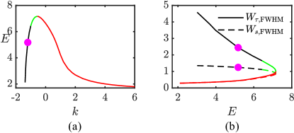
Figure 1: (a) The integral energy (7) for the family of stationary spatiotemporal solitons, obtained in the absence of the DM [$\Delta D=0$, $D_{\mathrm{av}}=1$ in Eq. (4)], versus the propagation constant, $k$. The critical point, with $dE/dk=0$, is located at $k=-0.55$. Solid black, red, and green curves represent, respectively, stable and unstable stationary solitons, and robust breathers. (b) The temporal, $W_{{\tau},\mathrm{FWHM}}$, and spatial, $W_{{s},\mathrm{FWHM}}$, FWHM widths of the stationary solitons (solid and dashed lines, respectively) versus $E$. The colors have the same meaning as in (a).

Results for the stability, displayed in Fig. 1, were verified by direct simulations of Eq. (3) for the evolution of the spatiotemporal solitons, performed by means of the split-step fast-Fourier-transform algorithm. An example, presented in Fig. 2 for the soliton with propagation constant $k=-1$ and energy $E=6.4364$, corroborates its stability, and displays its 3D shape. The propagation distance shown in Fig. 2 is tantamount to $\sim 200$ dispersion/diffraction lengths of the soliton. In the course of propagation, the soliton energy is conserved with relative accuracy $\sim 10^{-8}$, demonstrating that the soliton is an absolutely robust solution of the underlying DM model. In the absence of DM, the phase chirp of stable solitons remains equal to zero, in the course of the simulations.

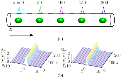
Figure 2: (a) The evolution of the stable spatiotemporal soliton with $k=-1.0$ and energy $E=6.4364$, in the system without DM [$\Delta D=0$, $D_{\mathrm{av}}=1$ in Eq. (4)], corresponding to the pink dot in Fig. 2. The evolution is shown by means of the set of isosurfaces of local intensity, $\left|u\left(x,y,\tau\right)\right|^{2}=0.8$, and its temporal profiles. (b) The evolution of the temporal (left) and spatial (right) local intensity.

II.2 Dispersion-managed spatiotemporal solitons

The main parameter which controls the action of DM in the temporal domain is the DM strength Nijhof ; book ; Turitsyn ,

$$S\equiv\left(D_{\mathrm{anom}}z_{\mathrm{anom}}+\left|D_{\mathrm{norm}}\right|z_{\mathrm{norm}}\right)/\left(W_{{\tau},\mathrm{FWHM}}^{2}\right)_{\min}~{}$$ (8)

where subscript $\min$ refers to the smallest value of the temporal width of the periodically oscillating DM soliton. To identify the temporal and spatial chirps of the soliton oscillating under the action of the DM, $C_{\tau}$ and $C_{s}$, it is represented in the Madelung’s form, as $u\left(x,y,\tau,z\right)\equiv\left|u\right|\exp\left(i\chi\right)$. Then, the chirps were computed from the numerically identified phase, $\chi\left(x,y,\tau,z\right)$, as

$$C_{\tau}=\frac{\partial^{2}}{\partial\tau^{2}}\chi\left(x=0,y=0,\tau,z\right)|_{\tau=0},$$

$$C_{s}=\frac{\partial^{2}}{\partial x^{2}}\chi\left(x,y=0,\tau=0,z\right)|_{x=0},~{}$$ (9)

The simulations of Eq. (3) with the DM map (4) were initiated with an input taken as stable stationary solitons numerically produced in the system without the DM (see above). It was found that the outcome of long-distance simulations is adequately determined by the value of the DM strength (8). First, for

$$S<S_{0}\approx 0.93$$ (10)

(relatively weak DM), the simulations produce quasi-stable 3D solitons, as shown in Fig. 3 for $S\approx 0.62$. While the soliton keeps its overall integrity and does not decay in the course of evolution (Fig. 3(d) demonstrates that, having passed $300$ DM periods, the soliton has lost $<1\%$ of the initial energy, through emission of small-amplitude radiation), it develops quasi-random oscillations of its characteristic parameters, although with a relatively small amplitude. This is seen in Fig. 3(c), that demonstrates a random walk of the soliton’s trajectory, which is trapped in a small domain of the plane of relevant dynamical parameters, viz., the temporal width and chirp.

It is relevant to mention that the spatiotemporal soliton displayed in Fig. 3(b) has the dispersion and diffraction lengths $\lesssim 1$. This is comparable to the underlying DM period, $z_{\mathrm{map}}=0.5$, which corroborates that the DM is an essential ingredient of the system under consideration. The same pertains to the completely stable spatiotemporal soliton displayed below in Fig. 4(b).

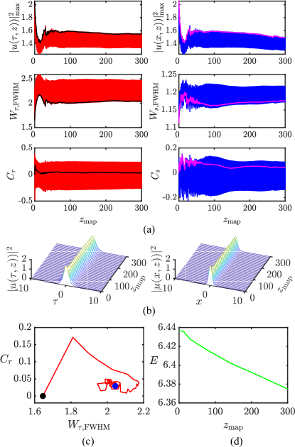
Figure 3: (a) The left column shows the evolution of the peak intensity, temporal width and chirp of a quasi-stable spatiotemporal soliton under the action of weak DM with strength $S=0.62$, corresponding to parameters $\Delta D=5$ and $D_{\mathrm{av}}=1$ in Eq. (4), over $300$ map periods (which corresponds to $z=150$; here and in other figures, values $z_{\mathrm{map}}$ refer to the propagation distance measured in units of the DM map). Black lines represent values of the same variables, taken at the beginning of each DM map (4). The input is the same stationary soliton which is shown in Fig. 2 in the absence of DM, with temporal width $W_{{\tau},\mathrm{FWHM}}\approx 1.65$. The right column displays the evolution of the soliton’s spatial width and chirp. Magenta lines represent their values at the beginning of each DM map. (b) Profiles of the oscillatory solitons in the temporal (left) and spatial (right) cross sections, plotted at the beginning of each DM map. (c) The trajectory of the soliton in the plane of the temporal width ($W_{{\ \tau},\mathrm{FWHM}}$) and chirp ($C_{\tau}$). Black and blue markers denote the initial and final points of the trajectory. (d) The total energy (7) of the soliton versus the propagation distance.

The boundary value (10) of the region of quasi-stable DM solitons corresponds, e.g., to the DM map with $\Delta D\approx 15$ (keeping $D_{\mathrm{av}}=1$), and temporal width $\left(W_{{\tau},\mathrm{FWHM}}\right)_{\min}\approx 2.84$. At $S>S_{0}$, the propagation of the spatiotemporal solitons is completely stable under the action of moderate or strong DM. A typical example is displayed in Fig. 4 for $S\approx 1.13$. The most essential manifestation of the full stability is that, in Fig. 4(d), the input loses $\simeq 7.5\%$ of its total energy at the initial stage of the evolution ($z<50$ DM periods), adjusting itself to the propagating state, and then, at $z>50$, the emission of radiation completely ceases. The fully regular dynamics of the soliton is also demonstrated by the evolution of its spatial and temporal parameters displayed in Fig. 4(a), cf. Fig. 3(a) for the quasi-stable spatiotemporal soliton.

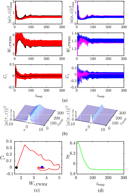
Figure 4: The same as in Fig. 3, and with the same input, but for the propagation of a stable spatiotemporal soliton under the action of moderately strong DM, with strength $S\approx 1.13$, corresponding to $\Delta D=30$ and $D_{\mathrm{av}}=1$ in Eq. (4).

Numerically exact DM solitons can be produced by means of the averaging method, which was previously elaborated for temporal solitons in dispersion-managed single-mode fibers Bennion ; Nijhof . The method is based on collecting a set of shapes of an oscillating soliton, produced by the straightforward simulations, at points where the shape is narrowest, and computing an average of the set. The result is the pulse which propagates in a strictly periodic form. A conclusion of further numerical analysis is that the direct simulations displayed in Fig. 4, as well as in other cases of the completely stable propagation, converge precisely to the DM solitons produced by the averaging method, extended to the present 3D setting. It is relevant to stress that the averaging procedure needs to be applied only in the temporal direction, while in the plane of $(x,y)$ the solution readily converges by itself to the one predicted by the averaging method. As an example, the DM soliton, to which the evolution displayed in Fig. 4 converges, is shown in Fig. 5. In Fig. 5(a), the isosurface plot at the top displays the spatiotemporal evolution of the DM soliton while it passes three DM maps, $0<z<1.5$, while other panels display the variation of the soliton’s temporal and spatial characteristics. In Fig. 5(b), the isosurface plot corroborates the full stability of the soliton over the propagation distance equivalent to $100$ maps.

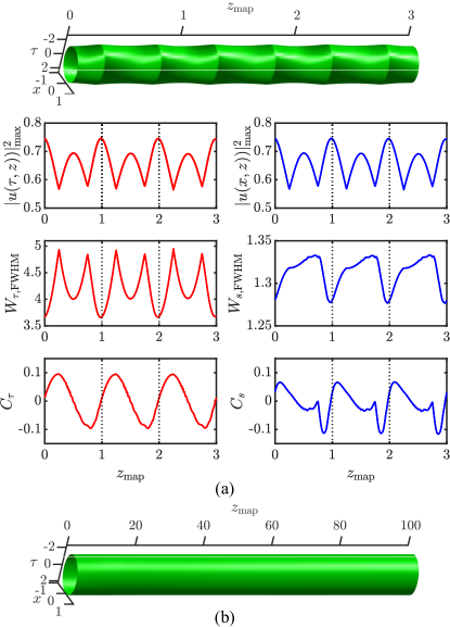
Figure 5: (a) The top panel displays the spatiotemporal dynamics of the numerically exact DM soliton, with strength $S\approx 1.13$ and minimum temporal width $\left(W_{{\tau}\mathrm{,FWHM}}\right)_{\min}\approx 3.65$, to which converges the soliton presented in Fig. 4. The evolution of the spatiotemporal DM soliton, produced by means of the averaging method (see the main text), is displayed by means of an isosurface of the local intensity, $\left|u\left(x,\tau,z\right)\right|^{2}=0.25$, in the cross section of $y=0$, as the soliton passes three DM maps, $0<z<1.5$. The bottom plots show the variation of the soliton’s temporal and spatial characteristics. (b) The isosurface of $\left|u\left(x,0,\tau,z\right)\right|^{2}=0.25$, shown at the beginning of each DM map, corroborates the full stability of the soliton as it passes $100$ DM periods, $0<z<50$.

II.3 Three-dimensional solitons with embedded vorticity

The creation of stable spatiotemporal DM solitons with embedded vorticity is a challenging objective. To the best of our knowledge, 3D solitons of such a type have not been reported before. To this end, it is necessary, first, to construct self-trapped vortex states as solutions to Eq. (3) in the absence of DM ($\Delta D=0$). In terms of the polar coordinates, $\left(r,\theta\right)$ in the plane of $\left(x,y\right)$, stationary vortex solitons are sought for as

$$u=\exp\left(im\theta\right)\phi(r,\tau),$$ (11)

with integer vorticity $m\geq 1$ and a localized real function $\phi$ obeying equation

$$k\phi-\frac{1}{2}\left(\frac{\partial^{2}}{\partial r^{2}}+\frac{1}{r}\frac{\partial}{\partial r}-\frac{m^{2}}{r^{2}}-\frac{1}{2}D_{\mathrm{av}}\frac{\partial^{2}}{\partial\tau^{2}}\right)\phi$$

$$+(x^{2}+y^{2})\phi-\phi^{3}=0,$$ (12)

with boundary condition $\phi\sim r^{m}$ at $r\rightarrow 0$. In the linear limit and for $D_{\mathrm{av}}=0$, $k$ is determined by energy eigenvalues of the 2D HO potential, i.e., $k_{\mathrm{linear}}=-\left(1+m\right)\sqrt{2}$.

A family of vortex-soliton solutions to Eq. (12) was constructed by means of the same Newton conjugate-gradient method which was used above for producing fundamental solitons, and the stability was explored through the computation of eigenvalues for modes of small perturbations. The result for $m=1$, similar to that reported in Ref. Boris for the NLSE with a strongly anisotropic HO trapping potential (i.e., the Gross-Pitaevskii equation), is displayed in Fig. 6. As seen in the figure, the Vakhitov-Kolokolov criterion, $dE/dk>0$, is necessary but not sufficient for the stability of the vortex solitons. An example of the stable vortex, shown by means of the isosurface of $\left|u\left(x,y,\tau\right)\right|^{2}$, clearly shows the inner hole, maintained in the soliton by the embedded vorticity. Unstable vortices follow the usual scenario, spontaneously splitting in a pair of fragments PhysD-vortices , as shown in Fig. 7. Eventually, the fragments merge into a quasi-turbulent state.

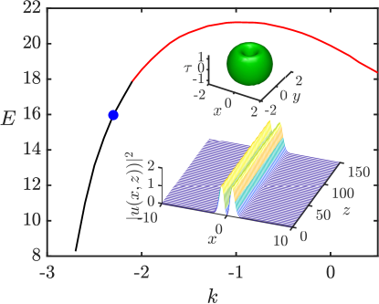
Figure 6: The energy of numerically generated vortex-soliton solutions of Eq. (3) with $D_{\mathrm{av}}=1$ and $m=1$ [see Eq. (11)], in the absence of DM ($\Delta D=0$), vs. the propagation constant. Black and red segments denote stable and unstable subfamilies, as identified through the computation of eigenvalues for small perturbations. The top inset shows the isosurface plot, $|u(x,y,\tau)|^{2}=0.35$, of a typical stable vortex soliton corresponding to the dot on the $E(k)$ curve, with $E=15.97$ and $k=-2.3$. The bottom inset: the stability of this soliton is illustrated by simulations of its perturbed evolution, displayed on the line of $y=\tau=0$. An example of unstable evolution of the vortex soliton, corresponding to $k=0$, is presented in Fig. 7.

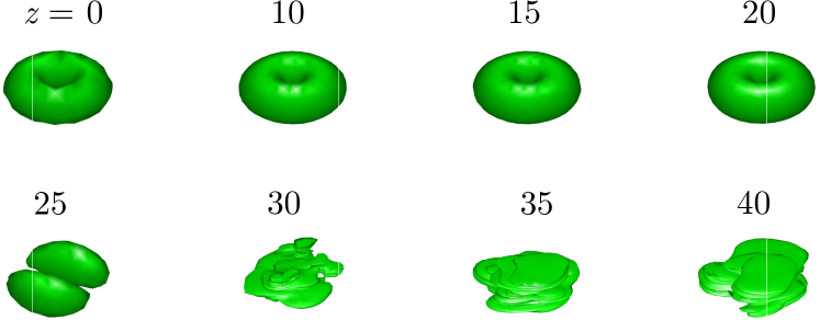
Figure 7: The isosurface evolution of an unstable vortex soliton with $m=1$, simulated in the framework of Eq. (3) with $\Delta D=0$ and $D_{\mathrm{av}}=1$. The input is a stationary solution of Eq. (12) for $k=0$, which is definitely unstable, as seen in Fig. 6.

In the presence of the DM, quasi-stable vortex solitons were found by direct simulations. A typical example is shown in Fig. 8: using a stable vortex from Fig. 6, which was found for $\Delta D=0$, as the input, direct simulations demonstrate the formation of a robust soliton which keeps the intrinsic vorticity and features slow shape oscillations with a large period, $\Delta z\simeq 80$ DM periods, under the action of the relatively strong DM, with $\Delta D=30$. The shape oscillations may be removed by accurately tuning the input, and a stability area for vortex solitons may be thus identified in the parameter space. Here, we do not aim to report such results in a comprehensive form, as it is extremely time-consuming to accumulate the necessary amount of numerical data. We did not consider vortex solitons with $m>1$ either, as it is known that, under the action of the 3D HO trapping potential, 3D solitons with multiple embedded vorticity are completely unstable, even in the absence of DM Boris ; PhysD-vortices .

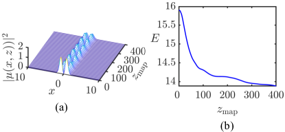
Figure 8: (a) Quasi-stable evolution of a vortex soliton with $m=1$, simulated in the framework of Eq. (3) with relatively strong DM, viz., $\Delta D=30$ and $D_{\mathrm{av}}=1$. The input is the stationary vortex soliton with $\Delta D=0$ and $D_{\mathrm{av}}=1$ shown in Fig. 6. (b) The total energy of the vortex soliton versus the propagation distance.

III Collisions between three-dimensional solitons

III.1 Collisions in the longitudinal direction

Once stable DM solitons have been found, it is relevant to consider collisions between them. The DM soliton can be set in longitudinal motion by the application of a kick (i.e., longitudinal boost) to it, with arbitrary frequency shift $\Omega$. Indeed, Eq. (3) is invariant with respect to the Galilean transformation, which generates a new solution from a given one, $u_{0}\left(x,y,\tau;z\right)$:

$$u\left(x,y,\tau;z\right)=\exp\left(-i\Omega\tau-\frac{i}{2}\Omega^{2}\int D(z)dz\right)$$

$$\times u_{0}\left(x,y,\tau-\tau_{0}+\Omega\int D(z)dz;z\right),$$ (13)

where $\tau_{0}$ is an arbitrary constant shift of the solution as a whole. Note that, in addition to the progressive motion with average speed

$$\mathrm{speed}=-D_{\mathrm{av}}\Omega,$$ (14)

the substitution of DM map (4) in Eq. (13) gives rise to oscillatory motion with spatial period $z_{\mathrm{map}}=0.5$ and temporal amplitude

$$\Delta\tau=(1/2)\Delta D|\Omega|z_{\mathrm{map}}~{}.$$ (15)

Thus, it is possible to create initial conditions for simulating collisions between spatiotemporal DM solitons moving in opposite temporal directions. In studies of temporal DM solitons in single-mode optical fibers, collisions were studied in detail for solitons carried by different wavelengths in the wavelength-division-multiplexed (WDM) system, which is an important practical problem, as the collision-induced jitter is a source of errors in data-transmission schemes coll1 ; coll2 .

Numerical simulations demonstrate elastic collisions between boosted solitons, created as per Eq. (13), with frequency shifts $\pm|\Omega|$ and centers initially set at points $\tau=\pm\tau_{0}$, see an example in Fig. 9 for $\Omega=\pm 0.3$. This “ slow” collision is strongly affected by the DM, because, with the smallest value of the solitons’ width $\left(W_{{\ \tau},\mathrm{FWHM}}\right)_{\min}\approx$ $3.65$ and relative speed $2D_{\mathrm{av}}|\Omega|=0.6$ [see Eq. (14)], the completion of the collision requires passing the propagation distance which is tantamount to more than $10$ DM periods: $Z_{\mathrm{coll}}\approx 2\left(W_{{\tau},\mathrm{FWHM}}\right)_{\min}/\left(2|\Omega|\right)\simeq 12z_{\text{{map}}}$. This estimate implies that multiple collisions take place between the two solitons, while they stay strongly overlapping. Indeed. Eq. (15) yields an estimate for the characteristic overlapping degree: $\left(W_{{\tau},\mathrm{FWHM}}\right)_{\min}/\Delta\tau\approx 1.62$ for the present values of parameters. This circumstance explains a complex intermediate structure observed at $z=16$ in Fig. 9(a), and in the left bottom plot of Fig. 9(b).

In addition to the initial temporal separation $2\tau_{0}$, a pair of colliding solitons is characterized by a phase shift between them, $\Delta\chi$. However, additional numerical results clearly demonstrate that, similar to what is well known in many other systems, results of the collisions do not depend on $\Delta\chi$. Actually, the collisions are driven by $\Delta\chi$ in the case when the initial pair is taken with zero relative velocity and relatively small separation Hulet , which is not the case here. Nevertheless, collisions displayed below in Fig. 11 are sensitive to the fact they start with $\Delta\chi=0$.

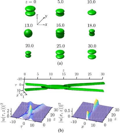
Figure 9: Simulations of slow collision, in the axial (temporal) direction, between two DM solitons, constructed as per Eq. (13) from the stable DM mode produced in Fig. 4 [with $\Delta D=30$, $D_{\mathrm{av}}=1$, $\left(W_{{\tau},\mathrm{FWHM}}\right)_{\min}\approx$ $3.65$]. The solitons, initially set at positions $\tau_{0}=\pm 5$, are boosted by frequency shifts $\Omega=\pm 0.3$. (a) A set of 3D snapshots, taken in the course of the collision, are depicted by means of isosurfaces of the local intensity, $\left|u\left(x,y,\tau\right)\right|^{2}$. (b) The collision shown by means of the isosurface in the cross section of $y=0$ (the top plot), and by the evolution of the intensity on the lines of $(x=y=0)$ and $(y=\tau=0)$ (the left and right bottom plots, respectively).

It is worthy to note that the collision produces, in a short interval of the propagation distance, a peak with a large amplitude, as seen in the left bottom panel of Fig. 9(b). This picture somewhat resembles the formation of optical rogue waves, see, e.g., recent work rogue and references therein. However, the analogy is rather superficial, as, unlike traditional rogue waves, here the peak appears not spontaneously, but as a result of the collision, it is not fed by a continuous-wave background, and the configuration is not intrinsically unstable (as it does not include a modulationally unstable background).

III.2 Collisions in the transverse direction

In the present context, it is relevant to consider, as a new option, collisions between 3D solitons moving in the transverse direction in the 3D setting. For this purpose, solitons may be set in motion by initially placing them at off-axis positions, with nonzero initial coordinates of the soliton’s centers, $\left(x_{0},y_{0}\right)$, and letting them roll down towards $x=y=0$ in the HO potential (a similar setup was employed to initiate collisions between matter-wave solitons trapped in the 3D isotropic HO potential Hulet ).

Thus, it is possible to consider the collision between two identical solitons initially shifted to positions $\pm\left(x_{0},y_{0}\right)$. It makes sense to address this possibility, first, in the absence of DM ($\Delta D=0$), as it was not addressed in previous works. As shown by a typical simulation displayed in Fig. 10, the colliding solitons, originally created (at $z=0$) at positions $x_{0}=y_{0}=\pm 3$, pass through each other quasi-elastically (QE) at $z\approx 1.1$, separate, then return under the action of the transverse HO potential, and again feature the QE collision at $z\approx 3.3$. The extension of the simulation demonstrates that the chain of QE collisions between the solitons, which perform the shuttle motion in the HO potential, continues indefinitely long, with intervals

$$\Delta z_{\mathrm{coll}}\approx 2.2$$ (16)

between the collisions. Note that, with the frequency of the trapping HO potential $\omega_{\perp}=\sqrt{2}$ in Eq. (12), the half-period of the shuttle motion in the HO potential is $\Delta z_{\mathrm{oscill}}=\pi/\omega_{\perp}\approx\allowbreak 2.22$, which readily explains the size of the interval between the collisions, see Eq. (16). Similar results were produced by simulations of head-on collisions between a soliton released from the initial position with coordinates $x_{0}=y_{0}>0$ and its quiescent counterpart placed on-axis (at $x_{0}=y_{0}=0$). Similar to what is mentioned above for collisions in the longitudinal direction, head-on collisions in the transverse plane are not sensitive to $\Delta\chi$ either.

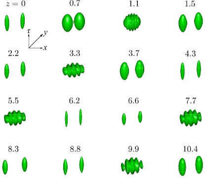
Figure 10: Collisions, in the transverse plane, between two 3D solitons in the absence of DM, i.e., with $\Delta=0$ and $D_{\mathrm{av}}=1$ in Eqs. (12) and (4). At $z=0$, the solitons, identical to the one presented in Fig. 2, are created at off-axis positions $x_{0}=y_{0}=\pm 3$. The dynamics of the collision is shown by means of the set of isosurfaces of the local intensity, $\left|u\left(x,y,\tau\right)\right|^{2}$. The quasi-elastic collisions between the solitons repeat periodically in the course of indefinitely long simulations.

It is also relevant to consider interactions between two solitons initially created with centers placed at points with coordinates $\left(x,y\right)=\pm\left(x_{0},y_{0}\right)$, additionally separated in the axial direction, i.e., with temporal coordinates $\tau=\pm\tau_{0}$. In this case, the solitons do not collide head-on; nevertheless, the simulation displayed in Fig. 11 demonstrates that the attractive interaction between the in-phase 3D solitons, mediated by their tails attraction , leads to the collision between them. As mentioned above, these collisions, unlike those displayed in Figs. 9 and 10, are sensitive to the fact that the solitons were created with zero initial phase difference, $\Delta\chi=0$; in the case of $\Delta\chi=\pi$, the collision does not take place, as the solitons interact repulsively (not shown here in detail). In this case, simulations also demonstrate a periodic chain of QE collisions with the same interval as predicted by Eq. (16). However, the corresponding full period of the collisional dynamics is double (including two collisions), $\Delta z_{\mathrm{coll}}^{\mathrm{(full)}}\approx 4.4$, because each collision leads to rotation of the line connecting centers of the solitons, as seen in Fig. 11.

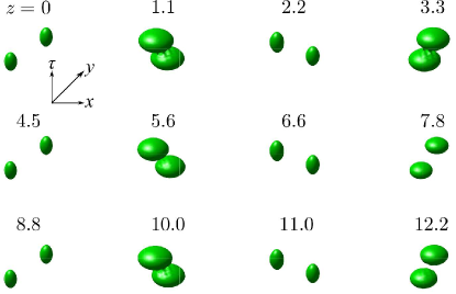
Figure 11: The same as in Fig. 10, but in the case when centers of the two in-phase solitons are initially separated in the axial direction by shifts $\tau_{0}=\pm 3$.

In the presence of the DM, collisions in the transverse direction are similar to those shown in Figs. 10 and 11. In particular, Fig. 12 demonstrates simulations of the head-on collision between the DM soliton, released from the position with $x_{0}=y_{0}=3$, and a quiescent one, placed at $x_{0}=y_{0}=0$. Note that, at the respective values of the parameters, the transverse speed of the soliton rolling down under the action of the HO potential at the collision moment is $\left(\mathrm{speed}\right)_{\perp}=-\omega_{\perp}\sqrt{x_{0}^{2}+y_{0}^{2}}=-5\sqrt{2}$. Then, the propagation distance necessary for the completion of the collision in the transverse direction can be estimated as

$$\left(\Delta z_{\mathrm{coll}}\right)_{\perp}\simeq 2W_{{\ s},\mathrm{FWHM}}/\left|\left(\mathrm{sp}\right)_{\perp}\right|\simeq 0.4,$$ (17)

where estimate $W_{{s},\mathrm{FWHM}}\simeq 1.3$ is taken from Fig. 4(b). The comparison of the value given by Eq. (17) with $z_{\mathrm{map}}=0.5$ suggests that the DM produces a moderate effect on the collisions, as corroborated by the comparison of Figs. 10 and 12. In any case, the collisions keep their QE character, recurring periodically with the interval correctly predicted by Eq. (16).

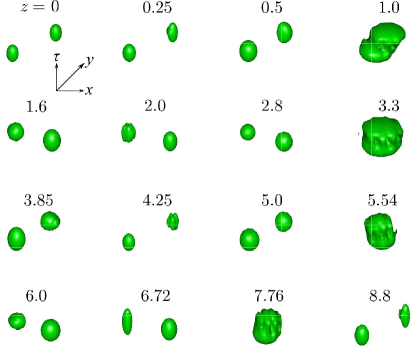
Figure 12: Collisions, in the transverse plane, between two 3D solitons in the presence of DM, with $\Delta D=30$ and $D_{\mathrm{av}}=1$ in Eqs. (12) and (4). At $z=0$, a DM soliton, the same as the one presented in Figs. 4 and 5, is placed at the position with $x_{0}=y_{0}=5$, and an identical soliton is placed at $x_{0}=y_{0}=0$. The dynamics of the collision is shown by means of the set of isosurfaces of the local intensity, $\left|u\left(x,y,\tau\right)\right|^{2}$. Quasi-elastic collisions between the solitons recur periodically in the course of the evolution.

As shown in Fig. 13, two DM solitons, initially taken with an additional temporal (axial) separation between them (therefore they cannot collide head-on), collide too, due to the mutual attraction, similar to what is shown above in Fig. 11 for the 3D solitons in the absence of DM. The interval between consecutive collisions is accurately predicted, as above, by Eq. (16), while, similar to what is observed in Fig. 11, the full period of the collisional dynamics is double, $\Delta z_{\mathrm{coll}}^{\mathrm{(full)}}\approx 4.4$, including two collisions, as the line connecting centers of the interacting solitons rotates, as a result of each collision. The comparison of Figs. 11 and (13) suggests that, as well as in the case of the head-on collision, DM produces a moderate effect on the interaction of the spatiotemporal solitons.

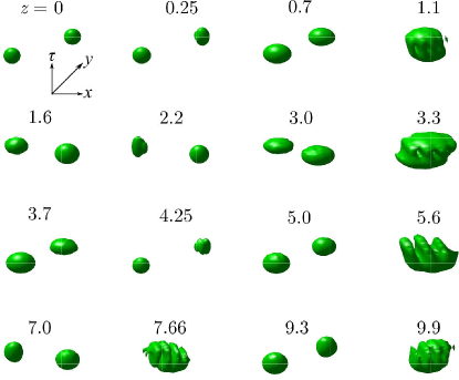
Figure 13: Recurring collisions between the same DM solitons as in Fig. 12, but initially placed at positions with coordinates $x_{0}=y_{0}=\tau_{0}=5$ and $x_{0}=y_{0}=\tau_{0}=0$, i.e., with the additional initial separation $\Delta\tau=5$ in the axial (temporal) direction.

IV Conclusion

The objective of this work is to extend the concept of DM (dispersion management) for 3D spatiotemporal solitons in multimode nonlinear optical fibers. In previous works, the DM concept was elaborated in detail, theoretically and experimentally, for 1D temporal solitons in single-mode fibers, as well as, in a theoretical form, for 2D spatiotemporal “ light bullets” in planar waveguides. We have here produced a family of 3D solitons in the model combining the GRIN structure of the refractive index in the transverse plane, approximated by the HO (harmonic-oscillator, i.e., quadratic) profile, Kerr self-focusing nonlinearity, and the usual DM map, based on periodic alternation of anomalous- and normal-GVD segments. It is found that the stability of the spatiotemporal DM solitons is determined by the DM strength parameter, $S$: periodically oscillating DM solitons self-trap from localized inputs, as fully stable modes, at $S>S_{0}\simeq 0.93$. After a transient rearrangement of the input, stable DM solitons keep constant energy. At $S<S_{0}$, the simulations demonstrate quasi-stability: the self-trapping gives rise to spatiotemporal solitons with persistent small-amplitude random intrinsic vibrations, which very slowly lose their energy, remaining robust over propagation distances corresponding to hundreds of DM periods. Stable three-dimensional DM solitons with embedded vorticity were constructed too. Collisions between DM solitons were considered by boosting them in opposite axial directions, with a conclusion that the collisions are quasi-elastic. Collisions in the transverse plane were also addressed, by initially placing one or both solitons at off-axis positions, and letting them roll down under the action of the HO potential. In this case, the pair of solitons, which perform the shuttle motion in the confining potential, demonstrate a periodic sequence of quasi-elastic collisions, in the absence or presence of DM.

The present work can be extended by considering the system including DM combined with the nonlinearity management. This extension may be relevant because different segments of multimode fibers in the composite waveguide may have different values of the nonlinearity parameter. As mentioned above, the realistic DM model may also include the intra-pulse stimulated-Raman-scattering effect and third-order dispersion, which deserves the consideration. Another direction for the development of the analysis may be the systems of the WDM type, with two or several distinct carrier wavelengths, modeled by a system of nonlinearly coupled NLSEs.

V Acknowledgments

We appreciate valuable discussions with T. Birks and L. G. Wright. This work was supported, in part, by the Thailand Research Fund (grant No. BRG 6080017), Israel Science Foundation (grant No. 1286/17), and Russian Foundation for Basic Research (grant No. 17-02-00081). TM acknowledges the support from Faculty of Engineering, Naresuan University, Thailand.

VI References

References

- (1) Malomed B A, Mihalache D, Wise D, and Torner L 2005 Journal of Optics B: Quantum and Semiclassical Optics 7 R53–R72
- (2) Malomed B A, Mihalache D, Wise D, and Torner L 2016 Journal of Physics B: Atomic, Molecular and Optical Physics 49 170502
- (3) Akhmediev N, Soto-Crespo J M, and Grelu P2007 Chaos 17 037112
- (4) Radu E and Volkov M S 2008 Physics Reports 468 101–105
- (5) Ackemann T, Firth W J, and Oppo G -L 2009 Advances In Atomic, Molecular, and Optical Physics 57 324–421
- (6) Chen Z, Segev M, and Christodoulides D N 2012 Reports on Progress in Physics 75 086401
- (7) Malomed B A 2016 The European Physical Journal Special Topics 225 2507–2532
- (8) Mihalache D 2017 Romanian Reports in Physics 69 403.
- (9) Veretenov N A, Fedorov S V, and Rosanov N N, 2017 Physical Review Letters 119 263901
- (10) Kartashov Y, Astrakharchik G, Malomed B A, and Torner L 2019 Nature Reviews Physics 1 185-197
- (11) Li B -X , Xiao B -X, Paladugu S, Shiyanovskii S V, and Lavrentovich O D 2019 Nature Communications 10 3749.
- (12) Kivshar Y S and Agrawal G P 2003 Optical Solitons: From Fibers to Photonic Crystals (Academic Press)
- (13) Pitaevskii L P and Stringari S 2003 Bose–Einstein Condensation (Oxford University Press)
- (14) Fibich G 2015 The Nonlinear Schrödinger Equation: Singular Solutions and Optical Collapse (Heidelberg: Springer)
- (15) Malomed B A (INVITED) 2019 Physica D 399 108–137
- (16) Malomed B A, Lederer F, Mazilu D, and Mihalache D2007 Physics Letters A 361 336-340
- (17) Silberberg Y 1990 Optics Letters 15 1282–1284
- (18) Cloge D 1972 Bell System Technical Journal 51 1767-1783
- (19) Ikeda M 1974 IEEE Journal of Quantum Electronics QE-10 362-371
- (20) Petermann K 1975 AEU - International Journal of Electronics and Communications 29 345-348
- (21) Crosignani B, Daino B, and DiPorto P 1975 Applied Physics Letters 27 237-239
- (22) Murphy K A, Gunther M F, Vengsarkar A M, and Claus R. 1991 Optics Letters 16 273-275
- (23) Nguyen L, Hwang D, Moon S, Moon D S, and Chung Y J 2008 Optics Express 16 11369-11375
- (24) Freund R E, Bunge C A, Ledentsov N N, Molin D, and Caspar C 2010 Journal of Lightwave Technology 28 569-586
- (25) Taubenblatt M A 2012 Journal of Lightwave Technology 30 448-458
- (26) Richardson D J, Fini J M, and Nelson L E 2013 Nature Photonics 7 354-362
- (27) Li G, Bai N, Zhao N, and Xia C 2014 Advances in Optics and Photonics 6 413-487
- (28) Saridis G M, Alexandropoulos D, Zervas G, and Simeonidou D 2015 IEEE Communications: Surveys and Tutorials 17 2136-2156
- (29) Carpenter J, Eggleton B J, and Schröder J, 2013 Optics Express 22 96–101
- (30) Yu S-S, Chien C-H, Lai Y, and Wang J 1995 Optics Communications 119 167–170
- (31) Chang R and Wang J 1993 Optics Letters 18 266–268
- (32) Raghavan R and Agrawal G P 2000 Optics Communication 180 377-382
- (33) Picozzi A, Millot G and Wabnitz S2015 Nature Photonics 9 289–291
- (34) Ahsan A S and Agrawal G P 2018 Optics Letters 43 3345–3348
- (35) Renninger W H and Wise F W 2013 Nature Communications 4 1719
- (36) Renninger W H and Wise F W 2014 Optica 1 101–104
- (37) Wright L G, S. Wabnitz S, Christodoulides D N, and Wise F W 2015 Physical Review Letters 115 223902
- (38) Wright L G, Renninger W H, Christodoulides D N, and Wise F W 2015 Optics Express 23 3492–3506
- (39) Florentin R, Kermene V, Benoist J, Desfarges-Berthelemot A, Pagnoux D, Barthélémy A, and Huignard J -P 2017 Light: Science & Applications 6 e16208
- (40) Guenard R, Krupa K, Dupiol R, Fabert M, Bendahmane A, Kermene V, Desfarges-Berthelemot A, Auguste J L, Tonello A, Barthélémy A, Millot G, Wabnitz S, and Couderc V, 2017 Optics Express 25 4783–4792
- (41) Tegin U and Ortaç B 2017 IEEE Photonics Technology Letters 29 2195–2198
- (42) Tzang O, Caravaca-Aguirre A M, and Piestun R 2018 Nature Photonics 12 368–374
- (43) Tegin U, Kakkava E, Rahmani B, Psaltis D, and Moser C 2019 Optica 6 1412–1415
- (44) Mayteevarunyoo T , Malomed B A, and Skryabin D V 2019 Optics Express 27 37364–37373
- (45) Malomed B A 2006 Soliton Management in Periodic Systems (Springer: New York).
- (46) Turitsyn S K, Bal B G, and Fedoruk M P 2012 Physics Reports 521 135–203
- (47) Gordon J P and Haus H A 1986 Optics Letters 11 665–667
- (48) Nakazawa M and Kubota H 1995 Japanese Journal of Applied Physics 34 L889-L891
- (49) Smith N J, Knox F M, Doran N J, Blow K J, and Bennion I 1996 Electronics Letters 32 54–55
- (50) Nijhof J H B, Doran N J, Forysiak W, and Knox F M 1997 Electronics Letters 33 1726–1727
- (51) Liang A H, Toda H, and Hasegawa A 1999 Optics Letters 24 799-801
- (52) Abdullaev F K, Baizakov B B, and Salerno M 2003 Physical Review E 68 066605
- (53) Matuszewski M, Trippenbach M, Malomed B A, Infeld E, and Skorupski M, 2004 Physical Review E 70 016603
- (54) Gao L, Wagner K H, and McLeod R R 2008 IEEE Journal of Selected Topics in Quantum Electronics 14 625–633
- (55) Kutz J N, Lynga C, and Eggleton B J 2005 Optics Express 13 3989–3998
- (56) Roati G, Zaccanti M, D’Errico C, Catani J, Modugno M, Simoni A, Inguscio M, and Modugno G 2007 Physical Review Letters 99 010403
- (57) Pollack S E, Dries D, Junker M, Chen Y P, Corcovilos T A, and Hulet R G 2009 Physical Review. Letters 102 090402
- (58) Towers I and Malomed B A 2002 Journal of the Optical Society of America B 19 537–543
- (59) Abdullaev F Kh, Caputo J G, Kraenkel A , and Malomed B A 2003 Physical Review A 67 013605
- (60) Saito H and Ueda M 2003 Physical Review Letters 90 040403
- (61) Montesinos G D, Pérez-García V M, and Michinel H 2004 Physical Review Letters 92 133901
- (62) Adhikari S K 2004 Physical Review A 69 063613
- (63) Nehmetallah G and Banerjee P P 2005 Journal of the Optical Society of America B 22 2200–2206
- (64) Itin A, Morishita T, and Watanabe S 2006 Physical Review A 74 033613
- (65) Matuszewski M, Infeld E, Malomed B A, and Trippenbach M 2005 Physical Review Letters 95 050403
- (66) Matsumoto T and Nakagawa K 1979 Applied Optics 18 14449-1454
- (67) Kashima N 1981 Applied Optics 20 859-3866
- (68) Goloborodko V, Keren S, Rosenthal A, Levit B, and Horowitz M 2003 Applied Optics 42 2284-2288
- (69) Zhao T, Gong Y, Rao Y J, Wu Y, Ran Z L, and Wu H 2011 Chinese Optics Letters 9 050602
- (70) Dong Z P, Li S J, Chen R S, Li H X, Gu C, Yao P J, and Xu L X 2019 Optics & Laser Technology 119 105576
- (71) Juarez A A, Krune E, Warm S, Bunge C A, and Petermann K 2014 Journal of Lightwave Technology 32 1549-1558
- (72) Mizunami T, Djambova T V, Niiho T, and Gupta A, 2000 Journal of Lightwave Technology 18 230-235
- (73) Chien C -H, Yu S -S, Lai Y, and Wang J 1996 Optics Communications 128, 145-157
- (74) Karlsson M, Anderson D, and Desaix M 1992 Optics Letters 17 22-24
- (75) Conforti M, Mas Arabi C, Mussot A, and Kudlinski A, 2017 Optics Letters 42 4004-4007
- (76) Wright L G, Sidorenko P, Pourbeyram H, Ziegler Z M, Isichenko A, Malomed B A, Menyuk C R, Christodoulides D N, and Wise F W, 2020 Nature Physics 16 565–570
- (77) Frantzeskakis D, Hizanidis K, Malomed B A, and Nistazakis H E, 1998 Pure and Applied Optics 7 L57–L62
- (78) Lakoba T I and Agrawal G P 1999 Journal of the Optical Society of America B 16 1332-1343
- (79) Lakoba T I and Kaup D J 1999 Optics Letters 24, 808-810
- (80) Yang J 2009 Journal of Computational Physics 228 7007–7024
- (81) Vakhitov N G and Kolokolov A A 1973 Radiophysics and Quantum Electronics 16 783–789
- (82) Bergé L 1998 Physics Reports 303 259–370
- (83) Niculae A N, Forysiak W, Gloag A J, Nijhof J H B, and Doran N J 1998 Optics Letters 23 1354–1356
- (84) Kaup D J, Malomed B A, and Yang J 1999 Journal of the Optical Society of America B 16 1628–1635
- (85) Nguyen J H V, Dyke P, Luo D, Malomed B A, and Hulet R G 2014 Nature Physics 10 918-922
- (86) Liu M, Li T -J, Luo A -P, Xu W -C, and Luo Z -C 2020 Photonics Research 8 246-251
- (87) Malomed B A 1998 Physical Review E 58 7928–7933