Gluon fragmentation into ${{}^{3}P_{J}^{[1,8]}}$ quark pair and
test of NRQCD factorization at two-loop level

Abstract

The next-to-leading order (NLO) ($\mathcal{O}(\alpha_{s}^{3})$) corrections for gluon fragmentation functions to a heavy quark-antiquark pair in ${{}^{3}P_{J}^{[1,8]}}$ states are calculated within the NRQCD factorization. We use integration-by-parts reduction and differential equations to semi-analytically calculate fragmentation functions in full-QCD, and find that infrared divergences can be absorbed by the NRQCD long distance matrix elements. Thus, the NRQCD factorization conjecture is verified at two-loop level via a physical process, which is free of artificial ultraviolet divergences. Through matching procedure, infrared-safe short distance coefficients and $\mathcal{O}(\alpha_{s}^{2})$ perturbative NRQCD matrix elements $\langle{\mathcal{O}}^{{{}^{3}P_{J}^{[1/8]}}}({{}^{3}S_{1}^{[8]}})\rangle_{\mathrm{NLO}}$ are obtained simultaneously. The NLO short distance coefficients are found to have significant corrections comparing with the LO ones.

1 Introduction

Heavy quarkonium provides an ideal physical system to explore the strong interaction, as the heavy quarkonium production contains both perturbative and non-perturbative effects in QCD. Non-relativistic QCD (NRQCD) factorization Bodwin:1994jh is the most widely used theory to explain quarkonium production so far. When transverse momentum $p_{T}$ of the produced quarkonium is large, fragmentation mechanism dominates and factorization is easier to hold, because long-distance interactions between quarkonium and initial-state particles are suppressed then.

Inclusive production differential cross section of a specific hadron $H$ at high $p_{T}$ can be calculated in collinear factorization Collins:1989gx ,

$$\mathrm{d}\sigma_{A+B\rightarrow H(p_{T})+X}=\sum_{i}\mathrm{d}\hat{\sigma}_{A+B\rightarrow i(p_{T}/z)+X^{\prime}}\otimes D_{i\to H}(z,\mu)+{\cal O}(1/p_{T}^{2})\,,$$ (1)

where $i$ sums over all quarks and gluons, $z$ is the light-cone momentum fraction carried by $H$ with respect to the parent parton $i$, and $A$ and $B$ are colliding particles whose effect should be further factorized into partons if they are hadrons. $d\hat{\sigma}_{A+B\rightarrow i(p_{T}/z)+X}$ are perturbatively calculable hard parts, while $D_{i\to H}(z,\mu)$ are non-perturbative but universal fragmentation functions (FFs) describing the probability of parton hadronizing to $H$ with momentum fraction $z$. For heavy quarkonium production, an important ${\cal O}(1/p_{T}^{2})$ contributions are double parton FFs which can also be factorized Kang:2011mg ; Kang:2014tta ; Kang:2014pya ; Fleming:2012wy ; Fleming:2013qu . In FFs, there is a collinear factorization scale $\mu$ dependence, which cancels with the similar dependence in hard parts perturbatively order by order, leaving physical differential cross section independent of the scale. The evolution of single parton FFs with respect to $\mu$ are controlled by the Dokshitzer-Gribov-Lipatov-Altarelli-Parisi (DGLAP) evolution equation Gribov:1972ri ; Altarelli:1977zs ; Dokshitzer:1977sg , and similar evolution equations for double parton FFs are calculated in Kang:2014tta . With these evolution equations, the only unknown information for FFs are their values at any chosen factorization scale $\mu=\mu_{f}$.

When $\mu_{f}$ is close to the quarkonium mass $m_{H}$, it is natural to calculate FFs via NRQCD factorization. For single parton FFs that will be considered in this paper, we have

$$D_{i\to H}(z,\mu_{f})=\sum_{n}d_{i\to Q\bar{Q}(n)}(z,\mu_{f})\langle\bar{{\mathcal{O}}}^{H}_{n}\rangle\,,$$ (2)

where $d_{i\to Q\bar{Q}(n)}$ represent the perturbative calculable short-distance coefficients (SDCs) to produce a heavy quark-antiquark pair $Q\bar{Q}$ with quantum number $n$, and $\langle\bar{{\mathcal{O}}}^{H}_{n}\rangle$ are normalized long-distance matrix elements (LDMEs) . The quantum number is usually expressed in spectroscopic notation $n={{}^{{2S+1}}L_{J}^{[c]}}$, with $c=1,8$ respectively for color-singlet state and color-octet state. According to velocity scaling rule Bodwin:1994jh , $\langle\bar{{\mathcal{O}}}^{H}_{n}\rangle$ is usually suppressed if $L$ is too large. Therefore, the most important states for phenomenological purpose are $S$-wave and $P$-wave states. Because LDMEs are supposed to be process independent, they can be determined by fitting experimental data, while SDCs can be calculated perturbatively through the matching procedure.

All the SDCs for single parton FFs to both $S$-wave and $P$-wave states up to $\mathcal{O}(\alpha_{s}^{2})$ are available Braaten:1993mp ; Braaten:1993rw ; Cho:1994gb ; Braaten:1994kd ; Beneke:1995yb ; Ma:1995vi ; Braaten:1996rp ; Braaten:2000pc ; Hao:2009fa ; Jia:2012qx ; Bodwin:2014bia (see Ma:2013yla ; Ma:2015yka for a summary and comparison). At $\alpha_{s}^{3}$ order, the leading order (LO) SDCs of $g\rightarrow Q\bar{Q}({{}^{3}S_{1}^{[1]}})+X$ and $g\rightarrow Q\bar{Q}({{}^{1}P_{1}^{[1]}})+X$ are calculated separately in Refs. Zhang:2017xoj ; Braaten:1993rw ; Braaten:1995cj ; Bodwin:2003wh ; Bodwin:2012xc and Ref. Sun:2018yam , and the next-to-leading order (NLO) SDCs of $g\to Q\bar{Q}({{}^{1}S_{0}^{[1,8]}})+X$ have also been calculated in Refs. Zhang:2018mlo ; Artoisenet:2018dbs ; Feng:2018ulg recently. To perform phenomenological analysis at a consistent precision, such as that for ${J/\psi}$ or $\chi_{cJ}$ production, at this order, one also needs the NLO SDCs of $g\rightarrow Q\bar{Q}({{}^{3}P_{J}^{[1,8]}})+X$ and the next-to-next-to-leading order (NNLO) SDCs of $g\rightarrow Q\bar{Q}({{}^{3}S_{1}^{[8]}})+X$. In this paper, we will focus on the former.

Another motivation to calculate the NLO FFs for processes $g\rightarrow Q\bar{Q}({{}^{3}P_{J}^{[1,8]}})+X$ is to test the NRQCD factorization conjecture at two-loop level with a physical process. The test at two-loop level exists in literature Nayak:2005rw ; Nayak:2005rt ; Nayak:2006fm ; Bodwin:2019bpf but within the framework of eikonal approximation for infrared (IR) divergences. The eikonal approximation introduces artificial ultraviolet (UV) divergences which makes the extraction of IR divergences beyond one-loop level highly nontrivial. Because we do not use eikonal approximation, the extraction of IR divergences in our case is straightforward.

In this paper, we aim to calculate NLO SDCs of $g\rightarrow Q\bar{Q}({{}^{3}P_{J}^{[1,8]}})+X$ to high precision using similar methods in our previous paper Zhang:2018mlo . The rest of the paper is organized as following. In Sec. 2, we calculate the process to LO and NLO in full-QCD. The calculation method is very similar to that in Ref. Zhang:2018mlo . A small improvement is the computation of operator renormalization shown in Sec. 2.3 and Appendix. A. We argue that the NRQCD factorization at two-loop level without eikonal approximation is verified in Sec. 2.4. The $\mathcal{O}(\alpha_{s}^{2})$ perturbative NRQCD matrix elements (PMEs) $\langle{\mathcal{O}}^{{{}^{3}P_{J}^{[1]}}}({{}^{3}S_{1}^{[8]}})\rangle_{\mathrm{NLO}}$ and $\langle{\mathcal{O}}^{{{}^{3}P_{J}^{[8]}}}({{}^{3}S_{1}^{[8]}})\rangle_{\mathrm{NLO}}$ are matched, and the corresponding IR-safe SDCs are obtained simultaneously in Sec. 3. Discussion will be presented in Sec. 4.

2 Full-QCD Calculation

2.1 Definition

FF of a gluon to a hadron (quarkonium) is defined by Collins and Soper Collins:1981uw ,

$$\begin{split}D_{g\rightarrow H}(z,\mu_{0})=&\frac{-g_{\mu\nu}z^{D-3}}{2\pi P_{c}^{+}(N_{c}^{2}-1)(D-2)}\int_{-\infty}^{+\infty}\mathrm{d}x^{-}e^{-iP_{c}^{+}x^{-}}\\ &\times\langle 0|G_{c}^{+\mu}(0)\mathcal{E}^{{\dagger}}(0,0,\bm{0}_{\perp})_{cb}\mathcal{P}_{H(P)}\mathcal{E}(0,x^{-},\bm{0}_{\perp})_{ba}G_{a}^{+\nu}(0,x^{-},\bm{0}_{\perp})|0\rangle\,,\end{split}$$ (3)

where $G^{\mu\nu}$ is the gluon field-strength operator, $P$ and $P_{c}$ are respectively the momenta of the produced hadron $H$ and the initial-state fragmenting gluon $g$, and $z=P^{+}/P_{c}^{+}$ is the ratio of momenta along the “+” direction. It is convenient to choose the frame in which the hadron has zero transverse momentum, $P=(zP_{c}^{+},M^{2}/(2zP_{c}^{+}),\bm{0}_{\perp})$, with $P^{2}=2P^{+}P^{-}=M^{2}$. The projection operator $\mathcal{P}_{H(P)}$ is defined by

$$\mathcal{P}_{H(P)}=\sum_{X}|H(P)+X\rangle\langle H(P)+X|\,,$$ (4)

where $X$ sums over all unobserved particles. The gauge link $\mathcal{E}(x^{-})$ is an eikonal operator that involves a path-ordered exponential of gluon field operators along a light-like path,

$$\mathcal{E}(0,x^{-},\bm{0}_{\perp})_{ba}=\mathrm{P}\,\text{exp}\left[+ig_{s}\int_{x^{-}}^{\infty}\mathrm{d}z^{-}A^{+}(0,z^{-},\bm{0}_{\perp})\right]_{ba}\,,$$ (5)

where $g_{s}=\sqrt{4\pi\alpha_{s}}$ is the QCD coupling constant and $A^{\mu}(x)$ is the matrix-valued gluon field in the adjoint representation: $[A^{\mu}(x)]_{ac}=if^{abc}A^{\mu}_{b}(x)$.

Since the SDCs $d$’s in the NRQCD factorization formula (2) are independent of the final state $H$, we can replace $H$ by on-shell $Q\bar{Q}$ states to extract $d_{i\to Q\bar{Q}[n]}$ through the matching procedure [See below (30) and (35)].

Choosing the factorization scale $\mu_{0}\sim 2m_{Q}$ with $m_{Q}$ being the heavy quark mass, we can calculate FF for $g\to Q\bar{Q}[n]$ in the full-QCD with the Feynman gauge. Most of the Feynman rules are the same as those of QCD, while the others related to the eikonal line can be found in Ref. Zhang:2018mlo . Feynman amplitudes are denoted as $\mathcal{M}_{\lambda_{{Q}}\lambda_{\bar{Q}}\lambda_{i}}(q)$, where $\lambda_{{Q}}$ and $\lambda_{\bar{Q}}$ are respectively spins of produced on-shell heavy quark and heavy antiquark, $\lambda_{i}$ ($i=1,2,\dots$) are spins of the initial-state virtual gluon or final-state unobserved light particles, and $q$ is the heavy quark momentum in the rest frame of heavy quark pair. To project the free $Q\bar{Q}$ pair to the state with spin-triplet and specific color, one can multiply amplitudes by projection operators and obtain

$$\mathcal{M}^{\alpha}_{\lambda_{i}}(q)=\text{Tr}\left[\Gamma_{c}\Gamma_{\lambda}^{\alpha}\overline{\mathcal{M}}_{\lambda_{{Q}}\lambda_{\bar{Q}}\lambda_{i}}(q)\right]\,,$$ (6)

where $\overline{\mathcal{M}}_{\lambda_{{Q}}\lambda_{\bar{Q}}\lambda_{i}}$ denotes amplitude with external heavy-(anti)quark spinors removed and the projection operators are defined as

$$\begin{split}&\Gamma_{c=1}=\frac{1}{\sqrt{N_{c}}}\,,\\ &\Gamma_{c=8}=\frac{\sqrt{2}T^{a}}{\sqrt{N_{c}^{2}-1}}\,,\\ &\Gamma_{\lambda}^{\alpha}=\frac{1}{\sqrt{2E}(E+m_{Q})}(\not{\overline{p}}-m_{Q})\frac{2E-\not{P}}{4E}\gamma^{\alpha}\frac{2E+\not{P}}{4E}(\not{p}-m_{Q})\,,\end{split}$$ (7)

where $p=P/2+q$ and $\overline{p}=P/2-q$ are momenta respectively for $Q$ and $\bar{Q}$, $m_{Q}$ is the mass of heavy quark, and $E$ is the energy of $Q$ or $\bar{Q}$ in the rest frame of $Q\bar{Q}$. With the on-shell conditions of $Q$ and $\bar{Q}$, we have

$$P\cdot q=0,\quad\quad P^{2}=4E^{2}=4(m_{Q}^{2}-q^{2}).$$ (8)

To project the amplitude into P-wave, we also need to take the derivation over $q^{\beta}$,

$$\mathcal{M}^{\alpha\beta}_{\lambda_{i}}=\frac{\partial}{\partial q^{\beta}}\mathcal{M}^{\alpha}_{\lambda_{i}}(q)|_{q\to 0}\,.$$ (9)

And by summing over spin and color of initial-state and final-state particles, we get the squared amplitude

$$\mathcal{A}_{J}=\frac{N_{\mathrm{CS}}}{N_{J}}\overline{\sum}P_{J}^{\alpha\alpha^{\prime}\beta\beta^{\prime}}\,\mathrm{Re}\left[\mathcal{M}^{\alpha\beta}_{\lambda_{i}}\mathcal{M}^{*\alpha^{\prime}\beta^{\prime}}_{\lambda_{i}}\right]\,,$$ (10)

where $N_{\mathrm{CS}}=\frac{z^{D-2}}{(N_{c}^{2}-1)(D-2)}$ with $D=4-2\epsilon$ is the space-time dimension. For different $J$, $N_{J}$ and $P_{J}^{\alpha\alpha^{\prime}\beta\beta^{\prime}}$ are respectively

$$N_{J}=\left\{\begin{aligned} &1\,,&\text{for }J=0\\ &\frac{1}{2}(D-1)(D-2)\,,&\text{for }J=1\\ &\frac{1}{2}(D+1)(D-2)\,,&\text{for }J=2\\ &(D-1)^{2}\,,&\text{for }\sum_{J}\end{aligned}\right.\,,$$ (11)

and

$$P_{J}^{\alpha\alpha^{\prime}\beta\beta^{\prime}}=\left\{\begin{aligned} &\frac{1}{D-1}I^{\alpha\beta}I^{\alpha^{\prime}\beta^{\prime}}\,,&\text{for }J=0\\ &\frac{1}{2}\left(I^{\alpha\alpha^{\prime}}I^{\beta\beta^{\prime}}-I^{\alpha\beta^{\prime}}I^{\alpha^{\prime}\beta}\right)\,,&\text{for }J=1\\ &\frac{1}{2}\left(I^{\alpha\alpha^{\prime}}I^{\beta\beta^{\prime}}-I^{\alpha\beta^{\prime}}I^{\alpha^{\prime}\beta}\right)-\frac{1}{D-1}I^{\alpha\beta}I^{\alpha^{\prime}\beta^{\prime}}\,,&\text{for }J=2\\ &I^{\alpha\alpha^{\prime}}I^{\beta\beta^{\prime}}\,,&\text{for }\sum_{J}\end{aligned}\right.\,,$$ (12)

where

$$I^{\alpha\beta}=-g^{\alpha\beta}+\frac{P^{\alpha}P^{\beta}}{P^{2}}\,.$$ (13)

Then, fragmentation function in the full-QCD can be denoted as

$$D[g\to Q\bar{Q}({{}^{3}P_{J}^{[1/8]}}])]=\int\mathrm{d}\Phi\mathcal{A}_{J}\,.$$ (14)

Here, $\mathrm{d}\Phi$ is the final-state phase space,

$$\mathrm{d}\Phi=\frac{P^{+}}{z^{2}S}\delta\left(\frac{1-z}{z}P^{+}-\sum_{i}k_{i}^{+}\right)\prod_{i}\frac{\mathrm{d}^{D}k_{i}}{(2\pi)^{D-1}}\delta_{+}(k_{i}^{2})\,,$$ (15)

where $S$ is the symmetry factor for final-state particles and $k_{i}$’s are momenta of final-state light particles. In the rest of the paper, we will take the case of $g\to Q\bar{Q}({{}^{3}P_{0}^{[1]}})+X$ as an explicit example to explain our calculations.

2.2 LO FFs

The Feynman diagrams of gluon fragmenting into $Q\bar{Q}[{{}^{3}P_{0}^{[1]}}]$ at the LO in $\alpha_{s}$ are shown in Figure 1.

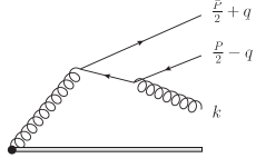
Figure 1: One of the two Feynman diagrams of gluon fragmenting into $Q\bar{Q}[{{}^{3}P_{0}^{[1]}}]$ at LO in $\alpha_{s}$. Another diagram can be obtained by permuting the heavy quark and anti-quark.

These diagrams can be easily calculated, and the obtained FF can be expressed as

$$D_{\mathrm{LO}}[g\to Q\bar{Q}({{}^{3}P_{0}^{[1]}})]=\frac{N_{\mathrm{LO}}}{1-\epsilon}\left[(1-z)^{-\epsilon}f_{1}(z)+(1-z)^{-1-2\epsilon}f_{2}(z)\right]\,,$$ (16)

where

$$N_{\mathrm{LO}}=\frac{\,\alpha_{s}^{2}}{(D-1)N_{c}m_{Q}^{5}}\left(\frac{\pi\mu_{r}^{2}}{m_{Q}^{2}}\right)^{\epsilon}\Gamma(1+\epsilon)$$ (17)

and

$$\begin{split}f_{1}(z)&=\frac{3(5-3z)}{\epsilon}+\frac{3}{2}(3z-4)-\frac{9z}{2}\epsilon\,,\\ f_{2}(z)&=\frac{3(1-z)(3z-5)}{\epsilon}+\frac{13z^{3}-42z^{2}+15z+18}{3}+2\left(2z^{2}-2z-1\right)z\epsilon+\frac{2z^{3}\epsilon^{2}}{3}\,.\end{split}$$ (18)

With the following decomposition

$$(1-z)^{-1-2\epsilon}=-\frac{\delta(1-z)}{2\epsilon}+\frac{1}{[1-z]_{+}}-2\epsilon\left[\frac{\ln(1-z)}{1-z}\right]_{+}+\mathcal{O}(\epsilon^{2})\,,$$ (19)

the FF can be expressed in the limit of $\epsilon\to 0$ as

$$\begin{split}D_{\mathrm{LO}}[g\to Q\bar{Q}({{}^{3}P_{0}^{[1]}})]=&N_{\mathrm{LO}}\Big{(}-\frac{2}{3\epsilon}\delta(1-z)+\frac{1}{3}\delta(1-z)+\frac{4}{3}\frac{z}{[1-z]_{+}}\\ &\phantom{N_{\mathrm{LO}}\Big{(}}+\frac{1}{6}(85-26z)z+3(5-3z)\ln(1-z)\Big{)}\,.\end{split}$$ (20)

It is clear that there is an IR divergence in the full-QCD result. This divergence can be absorbed by the color-octet PME, which will be explained in Sec. 3.

2.3 NLO FFs

The NLO full-QCD calculations of this process resemble closely to the NLO calculations of $g\to Q\bar{Q}({{}^{1}S_{0}^{[1,8]}})+X$ in Ref. Zhang:2018mlo . The relevant Feynman diagrams are shown in Figure 2 and Figure 3. In our calculation, we need to cut these diagrams at some specific positions. In Figure 4, we give an example to show how to obtain cut diagrams for the real and the virtual corrections.

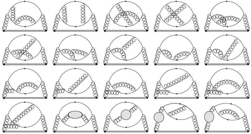
Figure 2: Typical Feynman diagrams without gluon eikonal vertex for $g\to Q\bar{Q}({{}^{3}P_{0}^{[1]}})+X$. The other diagrams can be obtained by permuting the heavy quark and anti-quark. The real and virtual diagrams can be obtained by cutting at different positions.

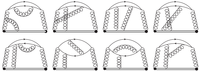
Figure 3: Typical Feynman diagrams with gluon eikonal vertex for $g\to Q\bar{Q}({{}^{3}P_{0}^{[1]}})+X$. The other diagrams can be obtained by permuting the heavy quark and anti-quark. The real and virtual diagrams can be obtained by cutting at different positions.

Figure 4: Real and virtual cut diagrams by cutting at different positions for the last diagrams in Figure 3.

The calculation is almost the same as that in Ref. Zhang:2018mlo . Firstly we generate the amplitude from the Feynman diagrams for real or virtual corrections. Then reduce them into linear combinations of master integrals (MIs). There are 95 MIs for real corrections and 66 MIs for virtual corrections. Fortunately, these MIs are the same as those in Ref. Zhang:2018mlo , which can be calculated by using differential equations (DEs) method Kotikov:1990kg ; Bern:1992em ; Remiddi:1997ny ; Gehrmann:1999as ; Henn:2013pwa ; Lee:2014ioa ; Adams:2017tga ; Caffo:2008aw ; Czakon:2008zk ; Mueller:2015lrx ; Lee:2017qql ; Liu:2017jxz ; Liu:2020kpc . We can estimate values of these MIs in regions $0\sim 1/4$, $1/4\sim 3/4$ and $3/4\sim 1$ respectively by the asymptotic expansions of them at $z=0,1/2$ and $1$. Finally, the real and virtual corrections can be expressed by asymptotic expansions in different regions as

$$\sum_{s}\sum_{i=0}^{n_{s}}(z-z_{0})^{s}\ln^{i}(z-z_{0})\sum_{j=0}^{\infty}I^{s\,i\,j}(\epsilon)(z-z_{0})^{j}\,,$$ (21)

where $s$ are linear functions of $\epsilon$, $n_{s}$ are integers determined by $s$, and coefficients $I^{s\,i\,j}(\epsilon)$ are functions of $\epsilon$, which can be computed to sufficient high order with high precision.

Renormalization has some differences from that in Ref. Zhang:2018mlo , because $1/\epsilon$ pole already presents at LO FF. Firstly, the on-shell renormalization constants of heavy quark field and mass ($\delta_{2}$ and $\delta_{m}$) should be expanded at least to $\mathcal{O}(\epsilon)$. To simplify the procedure, we use expression with exact $\epsilon$ dependence,

$$\delta_{i}=\frac{\alpha_{s}}{\pi}\Gamma(1+\epsilon)\left(\frac{\pi\mu_{r}^{2}}{m_{Q}^{2}}\right)^{\epsilon}\hat{\delta}_{i}\,,$$ (22)

with

$$\begin{split}\hat{\delta}_{2}&=-\frac{C_{F}}{4^{1-\epsilon}}\left(\frac{1}{\epsilon_{\mathrm{UV}}}\frac{1+2\epsilon}{1-2\epsilon}+\frac{2}{\epsilon_{\mathrm{IR}}}\right)\,,\\ \hat{\delta}_{m}&=-\frac{C_{F}}{4^{1-\epsilon}}\frac{1}{\epsilon_{\mathrm{UV}}}\frac{3-2\epsilon}{1-2\epsilon}\,,\end{split}$$ (23)

where $C_{F}=(N_{c}^{2}-1)/(2N_{c})$.

Apart from the calculations of the QCD counter terms, some tricks are needed in the calculation of operator renormalization. In the $\overline{\mathrm{MS}}$ scheme, the operator counter term is given by

$$D_{\mathrm{NLO}}^{\mathrm{Operator}}(z)=-\frac{\alpha_{s}}{2\pi}\frac{\Gamma(1+\epsilon)}{\epsilon}\left(\frac{4\pi\mu_{r}^{2}}{\mu_{0}^{2}}\right)^{\epsilon}\int_{z}^{1}\frac{\mathrm{d}y}{y}P_{gg}(y)D_{\mathrm{LO}}\left(\frac{z}{y}\right)\,,$$ (24)

where $\mu_{0}$ is the collinear factorization scale, and the Altarelli-Parisi splitting function $P_{gg}(z)$ is

$$P_{gg}(z)=b_{0}\,\delta(1-z)+2N_{c}\left(\frac{z}{(1-z)_{+}}+\frac{1-z}{z}+z(1-z)\right)\,,$$ (25)

where $b_{0}=(11N_{c}-2n_{f})/6$. If one takes the Eq. (20) as LO FF $D_{\mathrm{LO}}(z)$, there will be two plus functions convolved in the integral in (24), which is difficult to define and calculate. However, we can take Eq. (16) as the input form of the $D_{\mathrm{LO}}(z)$ to overcome this difficulty, with corresponding integrated results given in Appendix A. In this way, operator renormalization results can be easily obtained in each region, which are convenient to be added to the real and virtual corrections.

2.4 Verification of the NRQCD factorization at two-loop level

In the full-QCD calculations, the FF can be expressed by the phase space integral of amplitude squared as shown in Eq. (14). Before taking the derivative over $q$, the amplitude squared at ${\cal{O}}(q^{2})$ can be expressed as

$$\mathcal{A}(q,q^{\prime})=(q\cdot q^{\prime})\mathcal{A}_{1}+\frac{(q\cdot n)(q^{\prime}\cdot n)}{(P\cdot n)^{2}}\mathcal{A}_{2}\,,$$ (26)

where $n$ is the light-like vector that defines the direction of the eikonal line of fragmentation function. Because NRQCD LDMEs should be independent of the direction of the eikonal line of fragmentation function, and all remained IR divergences in full-QCD calculation must be absorbed into the LDMEs if NRQCD factorization is valid, there should be no IR divergences in $\mathcal{A}_{2}$. On the other hand, if one can show that there is no IR divergence in $\mathcal{A}_{2}$, then all IR divergences in full-QCD FF can be absorbed into the NRQCD LDMEs in principle, and the NRQCD factorization can be verified at two-loop level.

Two-loop verification of NRQCD factorization was also done in Refs. Nayak:2005rw ; Nayak:2005rt ; Nayak:2006fm ; Bodwin:2019bpf , in which eikonal approximation was used to simplify the calculation. The eikonal approximation however introduced artificial UV divergences that makes the extraction of IR divergences highly nontrivial.

In this subsection, we verify the NRQCD factorization without applying eikonal approximation. We take the process $g\to Q\bar{Q}({{}^{3}P_{J}^{[1]}})+X$ with $J$ summed as an example. To extract the part $\mathcal{A}_{2}$ only, we use the following projection operator

$$P_{qn}^{\alpha\alpha^{\prime}\beta\beta^{\prime}}=I^{\alpha\alpha^{\prime}}\left((D-2)I^{\beta\beta^{\prime}}-(D-1)d^{\beta\beta^{\prime}}\right)\,,$$ (27)

where

$$d^{\beta\beta^{\prime}}=-g^{\beta\beta^{\prime}}+\frac{P^{\beta}n^{\beta^{\prime}}+P^{\beta^{\prime}}n^{\beta}}{P\cdot n}-\frac{P^{2}n^{\beta}n^{\beta^{\prime}}}{(P\cdot n)^{2}}\,,$$ (28)

and we get

$$P_{qn}^{\alpha\alpha^{\prime}\beta\beta^{\prime}}\,\frac{\partial}{\partial q^{\beta}\,\partial q^{\prime\beta^{\prime}}}\mathcal{A}(q,q^{\prime})=I^{\alpha\alpha^{\prime}}(D-2)\frac{1}{P^{2}}\mathcal{A}_{2}\,.$$ (29)

Performing the calculations similar to those introduced in Sec. 2, we find that all divergences are canceled out after adding real corrections, virtual corrections as well as UV renormalization contributions. As a result, IR divergences in $\mathcal{A}(q,q^{\prime})$ are free of the gauge line vector $n$. Thus the NRQCD factorization is verified to hold at two-loop level, which is consistent with the observation in Refs. Nayak:2005rw ; Nayak:2005rt ; Nayak:2006fm ; Bodwin:2019bpf .

3 Matching procedure and the SDCs

As SDCs are independent of specifics of the hadronic states, we can match the $\mathcal{O}(\alpha_{s}^{2})$ PMEs from the divergences in full-QCD FFs and obtain the IR-safe SDCs simultaneously, thanks to the fact that NRQCD factorization holds at this order.

For $g\to Q\bar{Q}({{}^{3}P_{J}^{[1/8]}})$ process, the LO FF can be expressed by

$$\begin{split}D_{\mathrm{LO}}[g\to Q\bar{Q}({{}^{3}P_{J}^{[1/8]}})]=&\phantom{+}d_{\mathrm{LO}}[g\to Q\bar{Q}({{}^{3}P_{J}^{[1/8]}})]\langle{\mathcal{O}}^{{{}^{3}P_{J}^{[1/8]}}}({{}^{3}P_{J}^{[1/8]}})\rangle_{\mathrm{LO}}\\ &+d_{\mathrm{LO}}[g\to Q\bar{Q}({{}^{3}S_{1}^{[8]}})]\langle{\mathcal{O}}^{{{}^{3}P_{J}^{[1/8]}}}({{}^{3}S_{1}^{[8]}})\rangle_{\mathrm{LO}}\,,\end{split}$$ (30)

where $\langle{\mathcal{O}}^{{{}^{3}P_{J}^{[1]}}}({{}^{3}P_{J}^{[1]}})\rangle_{\mathrm{LO}}=\langle{\mathcal{O}}^{{{}^{3}P_{J}^{[8]}}}({{}^{3}P_{J}^{[8]}})\rangle_{\mathrm{LO}}=1$ is normalized. The LO SDC of gluon to ${{}^{3}S_{1}^{[8]}}$ in (30) has been calculated in Ref. Braaten:1996rp ; Braaten:2000pc , which is given in $D-$dimension by

$$d_{\mathrm{LO}}[g\to Q\bar{Q}({{}^{3}S_{1}^{[8]}})]=\frac{\pi\alpha_{s}\delta(1-z)}{(D-1)(N_{c}^{2}-1)m_{Q}^{3}}\,,$$ (31)

and the $\mathcal{O}(\alpha_{s})$ PMEs in the $\overline{\mathrm{MS}}$ subtraction scheme can be expressed as

$$\langle{\mathcal{O}}^{{{}^{3}P_{J}^{[1]}}}({{}^{3}S_{1}^{[8]}})\rangle_{\mathrm{LO}} =-C_{F}\frac{4\alpha_{s}}{3\pi m_{Q}^{2}}\frac{\Gamma(1+\epsilon)}{\epsilon_{\mathrm{IR}}}\left(\frac{4\pi\mu_{r}^{2}}{\mu_{\Lambda}^{2}}\right)^{\epsilon}\,,$$ (32)

$$\langle{\mathcal{O}}^{{{}^{3}P_{J}^{[8]}}}({{}^{3}S_{1}^{[8]}})\rangle_{\mathrm{LO}} =-B_{F}\frac{4\alpha_{s}}{3\pi m_{Q}^{2}}\frac{\Gamma(1+\epsilon)}{\epsilon_{\mathrm{IR}}}\left(\frac{4\pi\mu_{r}^{2}}{\mu_{\Lambda}^{2}}\right)^{\epsilon}\,,$$ (33)

where $B_{F}=(N_{c}^{2}-4)/(4N_{c})$ and $\mu_{\Lambda}$ is the NRQCD factorization scale. With full-QCD FF in Eq. (20), the $D-$dimension SDC $d_{\mathrm{LO}}[g\to Q\bar{Q}({{}^{3}P_{J}^{[1]}})]$ can be matched as

$$\begin{split}d_{\mathrm{LO}}[g\to Q\bar{Q}({{}^{3}P_{0}^{[1]}})]=&\frac{\,\alpha_{s}^{2}\Gamma(1+\epsilon)}{(D-1)N_{c}m_{Q}^{5}}\left(\frac{\pi\mu_{r}^{2}}{m_{Q}^{2}}\right)^{\epsilon}\times\Bigg{(}\left(\frac{1}{3}-\frac{2}{3}\ln\left(\frac{\mu_{\Lambda}^{2}}{4m_{Q}^{2}}\right)\right)\delta(1-z)\\ &+\frac{4}{3}\frac{z}{[1-z]_{+}}+\frac{1}{6}(85-26z)z+3(5-3z)\ln(1-z)\Bigg{)}\,,\end{split}$$ (34)

which equals to the finite part of the full-QCD FF in Eq. (20) if factorization scale is chosen as $\mu_{\Lambda}=2m_{Q}$. We find that the IR divergence in full-QCD FF $D_{\mathrm{LO}}[g\to Q\bar{Q}({{}^{3}P_{0}^{[1]}})]$ is absorbed into the $\mathcal{O}(\alpha_{s})$ PME $\langle{\mathcal{O}}^{{{}^{3}P_{J}^{[1]}}}({{}^{3}S_{1}^{[8]}})\rangle_{\mathrm{LO}}$, and the SDCs are IR-safe up to LO. This result is consistent with that in Ref. Ma:2013yla .

Similarly, $D_{\mathrm{NLO}}[g\to Q\bar{Q}({{}^{3}P_{J}^{[1/8]}})]$ can be expressed in the NRQCD factorization as

$$\begin{split}D_{\mathrm{NLO}}[g\to Q\bar{Q}({{}^{3}P_{J}^{[1/8]}})]=\phantom{+}&d_{\mathrm{NLO}}[g\to Q\bar{Q}({{}^{3}P_{J}^{[1/8]}})]\langle{\mathcal{O}}^{{{}^{3}P_{J}^{[1/8]}}}({{}^{3}P_{J}^{[1/8]}})\rangle_{\mathrm{LO}}\\ +&d_{\mathrm{LO}}[g\to Q\bar{Q}({{}^{3}P_{J}^{[1/8]}}))]\langle{\mathcal{O}}^{{{}^{3}P_{J}^{[1/8]}}}({{}^{3}P_{J}^{[1/8]}})\rangle_{\mathrm{NLO}}\\ +&d_{\mathrm{NLO}}[g\to Q\bar{Q}({{}^{3}S_{1}^{[8]}})]\langle{\mathcal{O}}^{{{}^{3}P_{J}^{[1/8]}}}({{}^{3}S_{1}^{[8]}})\rangle_{\mathrm{LO}}\\ +&d_{\mathrm{LO}}[g\to Q\bar{Q}({{}^{3}S_{1}^{[8]}})]\langle{\mathcal{O}}^{{{}^{3}P_{J}^{[1/8]}}}({{}^{3}S_{1}^{[8]}})\rangle_{\mathrm{NLO}}\,,\end{split}$$ (35)

where all LO terms are known. For NLO terms, $D_{\mathrm{NLO}}[g\to Q\bar{Q}({{}^{3}P_{J}^{[1/8]}})]$ are calculated in this work, $\langle{\mathcal{O}}^{{{}^{3}P_{J}^{[1/8]}}}({{}^{3}P_{J}^{[1/8]}})\rangle_{\mathrm{NLO}}$ are well-known, which have only Coulomb divergences and vanish in dimensional regularization with $\overline{\mathrm{MS}}$ subtraction scheme, and $d_{\mathrm{NLO}}[g\to Q\bar{Q}({{}^{3}S_{1}^{[8]}})]$ has been calculated in Refs. Braaten:2000pc ; Ma:2013yla , whose $D-$dimension form is given by

$$\begin{split}d_{\mathrm{NLO}}[g\to Q\bar{Q}({{}^{3}S_{1}^{[8]}})]=&\frac{\alpha_{s}^{2}\Gamma(1+\epsilon)}{4(D-1)C_{F}m_{Q}^{3}}\left(\frac{\pi\mu_{r}^{2}}{m_{Q}^{2}}\right)^{\epsilon}\Bigg{[}A(\mu_{r})\delta(1-z)+\frac{1}{N_{c}}P_{gg}(z)\times\\ &\left(\ln\left(\frac{\mu_{0}^{2}}{4m_{Q}^{2}}\right)-1\right)+\frac{2(1-z)}{z}-\frac{4(1-z+z^{2})^{2}}{2}\left[\frac{\ln(1-z)}{1-z}\right]_{+}\Bigg{]}\,,\end{split}$$ (36)

with

$$A(\mu_{r})=\frac{b_{0}}{N_{c}}\left(\ln\left(\frac{\mu_{r}^{2}}{4m_{Q}^{2}}\right)+\frac{13}{3}\right)+\frac{4}{N_{c}^{2}}-\frac{\pi^{2}}{3}+\frac{16}{3}\ln 2\,.$$ (37)

Therefore, SDCs $d_{\mathrm{NLO}}[g\to Q\bar{Q}({{}^{3}P_{J}^{[1/8]}})]$ and PMEs $\langle{\mathcal{O}}^{{{}^{3}P_{J}^{[1/8]}}}({{}^{3}S_{1}^{[8]}})\rangle_{\mathrm{NLO}}$ can be extracted from Eq. (35) thanks to the fact that the former one is finite and the later one is IR-divergent defined in $\overline{\mathrm{MS}}$ subtraction scheme.

The $\mathcal{O}(\alpha_{s}^{2})$ PMEs $\langle{\mathcal{O}}^{{{}^{3}P_{J}^{[1/8]}}}({{}^{3}S_{1}^{[8]}})\rangle_{\mathrm{NLO}}$ are obtained numerically with high precision. Using PSLQ algorithm ferguson1999analysis ; Bailey:1999nv , analytical expressions are obtained as

$$\langle{\mathcal{O}}^{{{}^{3}P_{J}^{[1]}}}({{}^{3}S_{1}^{[8]}})\rangle_{\mathrm{NLO}} =-C_{F}\frac{\alpha_{s}^{2}}{27\pi^{2}m_{Q}^{2}}\left(\frac{4\pi\mu_{r}^{2}}{\mu_{\Lambda}^{2}}\right)^{2\epsilon}\Gamma(1+\epsilon)^{2}\left(\frac{9b_{0}}{\epsilon^{2}}+\frac{5n_{f}+(12\pi^{2}-47)N_{c}}{\epsilon}\right)\,,$$ (38)

$$\langle{\mathcal{O}}^{{{}^{3}P_{J}^{[8]}}}({{}^{3}S_{1}^{[8]}})\rangle_{\mathrm{NLO}} =-B_{F}\frac{\alpha_{s}^{2}}{27\pi^{2}m_{Q}^{2}}\left(\frac{4\pi\mu_{r}^{2}}{\mu_{\Lambda}^{2}}\right)^{2\epsilon}\Gamma(1+\epsilon)^{2}\left(\frac{9b_{0}}{\epsilon^{2}}+\frac{5n_{f}+(3\pi^{2}-47)N_{c}}{\epsilon}\right)\,.$$ (39)

Setting factorization scales $\mu_{0}=\mu_{\Lambda}=2m_{Q}$, the NLO SDC can be expressed as

$$\begin{split}d_{\mathrm{NLO}}[g\to Q\bar{Q}({{}^{3}P_{0}^{[1]}})]=\frac{\alpha_{s}^{3}}{3\pi N_{c}m_{Q}^{5}}\Bigg{(}&p_{\delta}\delta(1-z)+\sum_{i=0}^{2}p_{i}\left[\frac{\ln^{i}(1-z)}{1-z}\right]_{+}+p(z)\\ &+\ln\left(\frac{\mu_{r}^{2}}{4m_{Q}^{2}}\right)b_{0}\,d_{\mathrm{LO}}[g\to Q\bar{Q}({{}^{3}P_{0}^{[1]}})]\Bigg{)}\,,\end{split}$$ (40)

where the coefficients $p_{\delta},p_{i}$ can be fitted with the PSLQ algorithm from high-precision numerical values as following

$$\begin{split}p_{\delta}&=\frac{95-24\pi^{2}}{162}n_{f}+\frac{756\zeta(3)+66\pi^{2}-1141-576\ln^{2}2-1032\ln 2}{324}N_{c}-\frac{2(4\ln 2-1)}{3}\frac{1}{N_{c}}\,,\\ p_{0}&=-n_{f}+\frac{-12\pi^{2}+119+64\ln 2}{18}N_{c}+\frac{8}{3}\frac{1}{N_{c}}\,,\\ p_{1}&=\frac{4}{9}n_{f}-\frac{64}{9}N_{c}\,,\\ p_{2}&=-\frac{16}{3}N_{c}\,,\end{split}$$ (41)

and $p(z)$ can be expressed as a piecewise function

$$p(z)=\left\{\begin{aligned} &\frac{63-8\pi^{2}}{36z}N_{c}+\sum_{i=0}^{2}\sum_{j=0}^{\infty}\ln^{i}z\,(2z)^{j}\left(A_{ij}^{f}\,n_{f}+A_{ij}\,N_{c}+\frac{A_{ij}^{N}}{N_{c}}\right)\,,&\text{for }0<z<\frac{1}{4}\\ &\sum_{j=0}^{\infty}(2z-1)^{j}\left(B_{j}^{f}\,n_{f}+B_{j}\,N_{c}+\frac{B_{j}^{N}}{N_{c}}\right)\,,&\text{for }\frac{1}{4}\leq z\leq\frac{3}{4}\\ &\sum_{i=0}^{3}\sum_{j=0}^{\infty}\ln^{i}(1-z)\,(2-2z)^{j}\,\left(C_{ij}^{f}\,n_{f}+C_{ij}\,N_{c}+\frac{C_{ij}^{N}}{N_{c}}\right)\,.&\text{for }\frac{3}{4}<z<1\end{aligned}\right.\,.$$ (42)

The coefficients $A_{ij}^{k},B_{j}^{k},C_{ij}^{k}$ can be evaluated numerically with high precision. In the attached ancillary file, we give these coefficients calculated up to $j=500$ to obtain the results with $140$-digit precision at any value of $z$.

The SDCs of $g\to Q\bar{Q}({{}^{3}P_{J}^{[1]}})+X$ with $J=1,2$ and $g\to Q\bar{Q}({{}^{3}P_{J}^{[8]}})+X$ with sum $J$ are calculated similarly, with results given as attachments in the ancillary file.

4 Numerical Results and Discussion

To see the effects of the NLO corrections, we choose parameters with $m_{b}=4.75\mathrm{~{}GeV}$, $N_{c}=3$, $n_{f}=4$, and $\alpha_{s}(\mu_{r}=2m_{b})=0.181$. In Figure 5, we plot the curves of LO SDCs and LO+NLO SDCs for the $P$-wave FFs with $\mu_{0}=\mu_{\Lambda}=2m_{b}$.

$g\to b\bar{b}({{}^{3}P_{0}^{[1]}})+X$

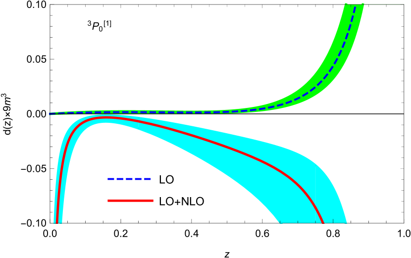
$g\to b\bar{b}({{}^{3}P_{1}^{[1]}})+X$

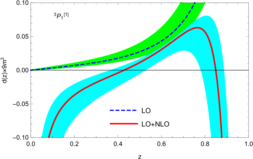
$g\to b\bar{b}({{}^{3}P_{2}^{[1]}})+X$

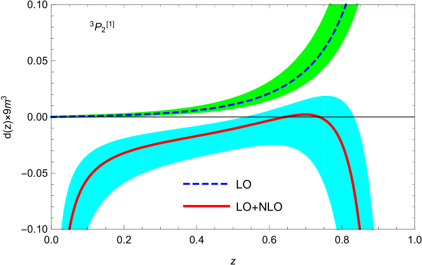
$g\to b\bar{b}({{}^{3}P_{J}^{[8]}})+X$

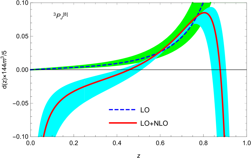
Figure 5: SDCs of the fragmentation functions of $g\to b\bar{b}({{}^{3}P_{J}^{[1/8]}}))+X$ at LO and NLO. The dashed line is for $d_{\mathrm{LO}}(z)\times c^{[1/8]}$, and the solid line is for $(d_{\mathrm{LO}}(z)+d_{\mathrm{NLO}}(z))\times c^{[1/8]}$, with scale choices $\mu_{r}=\mu_{0}=\mu_{\Lambda}=2m_{b}$, $c^{[1]}=9m_{b}^{5}$ for color-singlet and $c^{[8]}=144m_{b}^{5}/5$ for color-octet. The bands are obtained by varying the renormalization scale $\mu_{r}$ by a factor of 2.

The overall factor $9m_{b}^{5}$ for color-singlet and $144m_{b}^{5}/5$ for color-octet comes from normalization factors at NLO.

The sensitivities of LO and LO+NLO FFs with respective to the renormalization scale $\mu_{r}$ are illustrated Fig. 5 with bands corresponding to vary $\mu_{r}$ from $m_{b}$ to $4m_{b}$. We find that there are still large theoretical uncertainties after the NLO corrections.

With $\mu_{r}=\mu_{0}=\mu_{\Lambda}=2m_{b}$, we also provide K-factors (the ratio of LO+NLO over LO) for some special values of $z$ in Table 1 , where we find that the K-factors are negative for most values of $z$.

$z$	$K_{0}^{[1]}$	$K_{1}^{[1]}$	$K_{2}^{[1]}$	$K_{J}^{[8]}$
$0.10$	$-5.746823334$	$-24.60770220$	$-79.84997431$	$-38.52164437$
$0.15$	$-2.285338484$	$-10.32801893$	$-36.18197374$	$-17.35843659$
$0.20$	$-2.644346438$	$-5.288432534$	$-19.87280192$	$-9.481286949$
$0.25$	$-4.379318130$	$-2.914573185$	$-11.89225918$	$-5.572752664$
$0.30$	$-7.198593861$	$-1.593420613$	$-7.390964744$	$-3.288936921$
$0.35$	$-11.09174086$	$-0.7748378276$	$-4.639679071$	$-1.813295182$
$0.40$	$-15.40618698$	$-0.2304903644$	$-2.878388543$	$-0.8000547312$
$0.45$	$-17.98353020$	$0.1472252728$	$-1.722389454$	$-0.08193653748$
$0.50$	$-16.79362533$	$0.4131713893$	$-0.9577973668$	$0.4303450620$
$0.55$	$-13.06191610$	$0.5961117069$	$-0.4588481917$	$0.7878655480$
$0.60$	$-9.270458907$	$0.7101131977$	$-0.1500652088$	$1.020569545$
$0.65$	$-6.453740962$	$0.7593385828$	$0.01246796303$	$1.144600900$
$0.70$	$-4.605946556$	$0.7391584729$	$0.05021547782$	$1.164601499$
$0.75$	$-3.488264428$	$0.6339314219$	$-0.03511661296$	$1.072131730$
$0.80$	$-2.912955012$	$0.4091668085$	$-0.2661028908$	$0.8383434112$
$0.85$	$-2.799683132$	$-0.01116815401$	$-0.7094089942$	$0.3920893805$
$0.90$	$-3.226904801$	$-0.8227021717$	$-1.548987722$	$-0.4556362309$
$0.95$	$-4.779112355$	$-2.756468771$	$-3.481118189$	$-2.413493587$

Table 1: K-factors at different values of $z$. $K_{j}^{[c]}$ denotes the K-factor of $g\to Q\bar{Q}({{}^{3}P_{j}^{[c]}})+X$ and the symbol $J$ means the sum of $j=0,1,2$.

As shown in Figure 5, LO FFs are divergent at $z=1$. These divergences come from the $\delta(1-z)$ and $1/[1-z]_{+}$ terms in Eq. (34). Besides, the NLO FFs are negative and divergent at both $z=0$ and $z=1$. The leading behavior at $z\to 0$ is $1/z$, which means that the total fragmenting probability obtained by integrating the NLO FF over $z$ from $0$ to $1$ is divergent. But fortunately, physical cross sections are not sensitive to the behavior at $z\to 0$ after convolving FFs with partonic hard parts, which behave as $z^{n}$ in the small $z$ region with $n$ usually larger than $4$. As shown in Eq. (40), the divergences at $z\to 1$ behavior as $\delta(1-z)$ and plus functions with leading power $[\ln^{2}(1-z)/(1-z)]_{+}$, which comes from the expansion of $(1-z)^{-1-2\epsilon}\epsilon^{-2}$.

Obviously, the distribution of FF will not give us direct information about physical cross sections. To see the impact of the NLO results to the physical cross sections, we evaluate the $n$-th moments of the SDCs,

$$\int_{z_{0}}^{1}\mathrm{d}z\,z^{n}(d_{\mathrm{LO}}(z)+d_{\mathrm{NLO}}(z))\times c^{[1/8]}\,,$$ (43)

where $c^{[1]}=9m_{b}^{5}$ and $c^{[8]}=144m_{b}^{5}/5$. We plot the numerical results of integration K-factors with different $z_{0}$ and $n$, which are shown in Figure 6.

$g\to b\bar{b}({{}^{3}P_{0}^{[1]}})+X$

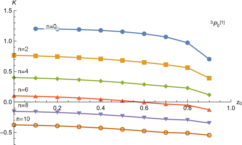
$g\to b\bar{b}({{}^{3}P_{1}^{[1]}})+X$

$g\to b\bar{b}({{}^{3}P_{2}^{[1]}})+X$

$g\to b\bar{b}({{}^{3}P_{J}^{[8]}})+X$

Figure 6: The K-factors calculated by the integration results with Eq. (43) for different $z_{0}$ and $n$.

We find that for the same $n$, the K-factors are quite steady for different $z_{0}$, meaning that cross sections are dominated by FFs at large $z$. Besides, the K-factors decrease with the increase of $n$. Especially, the color-singlet K-factors become negative for large $n$. And there may be a cancellation between the LO and the NLO FFs at about $7$-th moment for color-singlet quarkonium productions. Further more, it is clear that though the K-factors and values of FFs at each position $z=z_{0}$ are quite different for $j=0,1,2$ as shown in Table 1 and in Figure 5, they are almost the same in the sense of integration as shown in Figure 6.

For the special case $z_{0}=0$, we can estimate the impact of NLO calculations on physical cross sections. The numerical results are shown in Table 2.

state	SDCs$*c^{[1/8]}$	$z^{2}$	$z^{4}$	$z^{6}$	$z^{8}$	$z^{10}$
${{}^{3}P_{0}^{[1]}}$	LO	$-0.128268$	$-0.135763$	$-0.141953$	$-0.147253$	$-0.151898$
	LO+NLO	$-0.0982734$	$-0.0544311$	$-0.0143470$	$0.0226121$	$0.0570568$
	K-factor	$0.766154$	$0.400927$	$0.101068$	$-0.153559$	$-0.375626$
${{}^{3}P_{1}^{[1]}}$	LO	$-0.0860886$	$-0.102339$	$-0.114018$	$-0.123176$	$-0.130722$
	LO+NLO	$-0.0735848$	$-0.0436727$	$-0.0119884$	$0.0195102$	$0.0501917$
	K-factor	$0.854756$	$0.426745$	$0.105145$	$-0.158393$	$-0.383957$
${{}^{3}P_{2}^{[1]}}$	LO	$-0.106291$	$-0.118021$	$-0.126989$	$-0.134287$	$-0.140456$
	LO+NLO	$-0.0872125$	$-0.0507874$	$-0.0152633$	$0.0187392$	$0.0511634$
	K-factor	$0.820505$	$0.430326$	$0.120194$	$-0.139546$	$-0.364266$
${{}^{3}P_{J}^{[8]}}$	LO	$-0.101999$	$-0.114765$	$-0.124328$	$-0.132024$	$-0.138483$
	LO+NLO	$-0.211825$	$-0.196364$	$-0.173108$	$-0.147720$	$-0.121978$
	K-factor	$2.07674$	$1.71101$	$1.39235$	$1.11888$	$0.880816$

Table 2: Moments and K-factors of SDCs.

For large $n$, the influence of the behavior at $z\to 1$ becomes more and more prominent and the NLO correction becomes more and more significant. In addition, the K-factors of color-octet process are much larger than those of color-singlet process.

The above discussion implies that resummation at large $z$ region may be crucial. This can be done within the framework of soft gluon factorization Ma:2017xno , which we leave for future study.

Appendix A Operator renormalization integrals

The operator convolution integration is shown in Eq. (24) with the splitting functions shown in Eq. (25). The splitting functions can be divided into three parts, while the LO FF have two regions. Thus there are $6$ types of integrals,

$$\int_{z}^{1}\frac{\mathrm{d}y}{y}\delta(1-y)(1-\frac{z}{y})^{-\epsilon}f_{1}\left(\frac{z}{y}\right)=\lambda^{-\epsilon}f_{1}(1-\lambda)\,,$$ (44)

$$\int_{z}^{1}\frac{\mathrm{d}y}{y}\delta(1-y)(1-\frac{z}{y})^{-1-2\epsilon}f_{2}\left(\frac{z}{y}\right)=\lambda^{-1-2\epsilon}f_{2}(1-\lambda)\,,$$ (45)

$$\begin{split}&\int_{z}^{1}\frac{\mathrm{d}y}{y}g(y)(1-\frac{z}{y})^{-\epsilon}f_{1}\left(\frac{z}{y}\right)\\ &=\lambda^{-\epsilon}\int_{0}^{1}\mathrm{d}yh(y,\epsilon)\frac{\lambda}{1-\lambda y}g\left(\frac{1-\lambda}{1-\lambda y}\right)f_{1}(1-\lambda y)\,,\end{split}$$ (46)

$$\begin{split}&\int_{z}^{1}\frac{\mathrm{d}y}{y}g(y)(1-\frac{z}{y})^{-1-2\epsilon}f_{2}\left(\frac{z}{y}\right)\\ &=\lambda^{-1-2\epsilon}\Bigg{[}-\frac{1}{2\epsilon}\lambda g(1-\lambda)f_{2}(1)\\ &\phantom{=}+\int_{0}^{1}\frac{\mathrm{d}y}{y}h(y,2\epsilon)\left(\frac{\lambda}{1-\lambda y}g\left(\frac{1-\lambda}{1-\lambda y}\right)f_{2}(1-\lambda y)-\lambda g(1-\lambda)f_{2}(1)\right)\Bigg{]}\,,\end{split}$$ (47)

$$\begin{split}&\int_{z}^{1}\frac{\mathrm{d}y}{y}\frac{1}{[1-y]_{+}}(1-\frac{z}{y})^{-\epsilon}f_{1}\left(\frac{z}{y}\right)\\ &=\lambda^{-\epsilon}\ln\lambda\,f_{1}(1-\lambda)+\lambda^{-\epsilon}\int_{0}^{1}\frac{\mathrm{d}y}{1-y}\left(h(y,\epsilon)f_{1}(1-\lambda y)-\frac{1-\lambda}{1-\lambda y}f_{1}(1-\lambda)\right)\,,\end{split}$$ (48)

$$\begin{split}&\int_{z}^{1}\frac{\mathrm{d}y}{y}\frac{1}{[1-y]_{+}}(1-\frac{z}{y})^{-1-2\epsilon}f_{2}\left(\frac{z}{y}\right)\\ &=\lambda^{-1-2\epsilon}\ln\lambda\,f_{2}(1-\lambda)\\ &\phantom{=}+\lambda^{-1-2\epsilon}\Bigg{[}\left(-\frac{1}{2\epsilon}-H(-2\epsilon)-\ln(1-\lambda)\right)f_{2}(1)\\ &\phantom{=}+\int_{0}^{1}\frac{\mathrm{d}y}{1-y}\left(h(y,2\epsilon)\frac{f_{2}(1-\lambda y)-f_{2}(1)}{y}-\frac{1-\lambda}{1-\lambda y}\left(f_{2}(1-\lambda)-f_{2}(1)\right)\right)\Bigg{]}\,,\end{split}$$ (49)

where $\lambda=1-z$, $g(y)=(1-2y)/y+y(1-y)$ comes from the splitting function, $H(-2\epsilon)$ is the Harmonic number which can be expanded in the limit of $\epsilon\to 0$ and

$$h(y,\epsilon)=y^{-\epsilon}=\sum_{i}\frac{(-\epsilon)^{i}}{i!}\ln^{i}(y)$$ (50)

is the Taylor series at $\epsilon\to 0$. Based on these results, we find that two more behaviors $(1-z)^{-\epsilon}\ln(1-z)$ and $(1-z)^{-1-2\epsilon}\ln(1-z)$ are added to the region at $z\to 1$.

- (1) G. T. Bodwin, E. Braaten, and G. P. Lepage, Rigorous QCD analysis of inclusive annihilation and production of heavy quarkonium, Phys. Rev. D51 (1995) 1125–1171 [hep-ph/9407339] [InSPIRE]. [Erratum: Phys. Rev.D55,5853(1997)].
- (2) J. C. Collins, D. E. Soper, and G. Sterman, Factorization of Hard Processes in QCD, Adv.Ser.Direct.High Energy Phys. 5 (1988) 1–91 [hep-ph/0409313] [InSPIRE].
- (3) Z.-B. Kang, J.-W. Qiu, and G. Sterman, Heavy quarkonium production and polarization, Phys.Rev.Lett. 108 (2012) 102002 [arXiv:1109.1520] [InSPIRE].
- (4) Z.-B. Kang, Y.-Q. Ma, J.-W. Qiu, and G. Sterman, Heavy quarkonium production at collider energies: Factorization and Evolution, Phys.Rev. D90 (2014) 034006 [arXiv:1401.0923] [InSPIRE].
- (5) Z.-B. Kang, Y.-Q. Ma, J.-W. Qiu, and G. Sterman, Heavy Quarkonium Production at Collider Energies: Partonic Cross Section and Polarization, Phys.Rev. D91 (2015) 014030 [arXiv:1411.2456] [InSPIRE].
- (6) S. Fleming, A. K. Leibovich, T. Mehen, and I. Z. Rothstein, The Systematics of Quarkonium Production at the LHC and Double Parton Fragmentation, Phys.Rev. D86 (2012) 094012 [arXiv:1207.2578] [InSPIRE].
- (7) S. Fleming, A. K. Leibovich, T. Mehen, and I. Z. Rothstein, Anomalous dimensions of the double parton fragmentation functions, Phys.Rev. D87 (2013) 074022 [arXiv:1301.3822] [InSPIRE].
- (8) V. Gribov and L. Lipatov, Deep inelastic e p scattering in perturbation theory, Sov.J.Nucl.Phys. 15 (1972) 438–450 [InSPIRE].
- (9) G. Altarelli and G. Parisi, Asymptotic Freedom in Parton Language, Nucl.Phys. B126 (1977) 298 [InSPIRE].
- (10) Y. L. Dokshitzer, Calculation of the Structure Functions for Deep Inelastic Scattering and Annihilation by Perturbation Theory in Quantum Chromodynamics., Sov.Phys.JETP 46 (1977) 641–653 [InSPIRE].
- (11) E. Braaten, K. Cheung, and T. C. Yuan, decay into charmonium via charm quark fragmentation, Phys.Rev. D48 (1993) 4230–4235 [hep-ph/9302307] [InSPIRE].
- (12) E. Braaten and T. C. Yuan, Gluon fragmentation into heavy quarkonium, Phys.Rev.Lett. 71 (1993) 1673–1676 [hep-ph/9303205] [InSPIRE].
- (13) P. L. Cho, M. B. Wise, and S. P. Trivedi, Gluon fragmentation into polarized charmonium, Phys. Rev. D51 (1995) R2039–R2043 [hep-ph/9408352] [InSPIRE].
- (14) E. Braaten and T. C. Yuan, Gluon fragmentation into P wave heavy quarkonium, Phys.Rev. D50 (1994) 3176–3180 [hep-ph/9403401] [InSPIRE].
- (15) M. Beneke and I. Z. Rothstein, Psi-prime polarization as a test of color octet quarkonium production, Phys. Lett. B372 (1996) 157–164 [hep-ph/9509375] [InSPIRE]. [Erratum: Phys. Lett.B389,769(1996)].
- (16) J. P. Ma, Quark fragmentation into p wave triplet quarkonium, Phys. Rev. D53 (1996) 1185–1190 [hep-ph/9504263] [InSPIRE].
- (17) E. Braaten and Y.-Q. Chen, Dimensional regularization in quarkonium calculations, Phys.Rev. D55 (1997) 2693–2707 [hep-ph/9610401] [InSPIRE].
- (18) E. Braaten and J. Lee, Next-to-leading order calculation of the color octet 3S(1) gluon fragmentation function for heavy quarkonium, Nucl. Phys. B586 (2000) 427–439 [hep-ph/0004228] [InSPIRE].
- (19) G. Hao, Y. Zuo, and C.-F. Qiao, The Fragmentation Function of Gluon Splitting into P-wave Spin-singlet Heavy Quarkonium, [arXiv:0911.5539] [InSPIRE].
- (20) Y. Jia, W.-L. Sang, and J. Xu, Inclusive Production at Factories, Phys. Rev. D86 (2012) 074023 [arXiv:1206.5785] [InSPIRE].
- (21) G. T. Bodwin, H. S. Chung, U.-R. Kim, and J. Lee, Quark fragmentation into spin-triplet -wave quarkonium, Phys. Rev. D91 (2015) 074013 [arXiv:1412.7106] [InSPIRE].
- (22) Y.-Q. Ma, J.-W. Qiu, and H. Zhang, Heavy quarkonium fragmentation functions from a heavy quark pair. I. wave, Phys.Rev. D89 (2014) 094029 [arXiv:1311.7078] [InSPIRE].
- (23) Y.-Q. Ma, J.-W. Qiu, and H. Zhang, Fragmentation functions of polarized heavy quarkonium, JHEP 06 (2015) 021 [arXiv:1501.04556] [InSPIRE].
- (24) P. Zhang, Y.-Q. Ma, Q. Chen, and K.-T. Chao, Analytical calculation for the gluon fragmentation into spin-triplet S-wave quarkonium, Phys. Rev. D96 (2017) 094016 [arXiv:1708.01129] [InSPIRE].
- (25) E. Braaten and T. C. Yuan, Gluon fragmentation into spin triplet S wave quarkonium, Phys. Rev. D52 (1995) 6627–6629 [hep-ph/9507398] [InSPIRE].
- (26) G. T. Bodwin and J. Lee, Relativistic corrections to gluon fragmentation into spin triplet S wave quarkonium, Phys. Rev. D69 (2004) 054003 [hep-ph/0308016] [InSPIRE].
- (27) G. T. Bodwin, U.-R. Kim, and J. Lee, Higher-order relativistic corrections to gluon fragmentation into spin-triplet S-wave quarkonium, JHEP 1211 (2012) 020 [arXiv:1208.5301] [InSPIRE].
- (28) Q.-F. Sun, Y. Jia, X. Liu, and R. Zhu, Inclusive production and energy spectrum from annihilation at a super factory, Phys. Rev. D98 (2018) 014039 [arXiv:1801.10137] [InSPIRE].
- (29) P. Zhang, C.-Y. Wang, X. Liu, Y.-Q. Ma, C. Meng, and K.-T. Chao, Semi-analytical calculation of gluon fragmentation into1S quarkonia at next-to-leading order, JHEP 04 (2019) 116 [arXiv:1810.07656] [InSPIRE].
- (30) P. Artoisenet and E. Braaten, Gluon fragmentation into quarkonium at next-to-leading order using FKS subtraction, JHEP 01 (2019) 227 [arXiv:1810.02448] [InSPIRE].
- (31) F. Feng and Y. Jia, Next-to-leading-order QCD corrections to gluon fragmentation into quarkonia, [arXiv:1810.04138] [InSPIRE].
- (32) G. C. Nayak, J.-W. Qiu, and G. F. Sterman, Fragmentation, factorization and infrared poles in heavy quarkonium production, Phys. Lett. B 613 (2005) 45–51 [hep-ph/0501235].
- (33) G. C. Nayak, J.-W. Qiu, and G. Sterman, Fragmentation, NRQCD and NNLO factorization analysis in heavy quarkonium production, Phys.Rev. D72 (2005) 114012 [hep-ph/0509021] [InSPIRE].
- (34) G. C. Nayak, J.-W. Qiu, and G. F. Sterman, NRQCD Factorization and Velocity-dependence of NNLO Poles in Heavy Quarkonium Production, Phys. Rev. D 74 (2006) 074007 [hep-ph/0608066].
- (35) G. T. Bodwin, H. S. Chung, J.-H. Ee, U.-R. Kim, and J. Lee, Covariant calculation of a two-loop test of nonrelativistic QCD factorization, Phys. Rev. D 101 (2020) 096011 [arXiv:1910.05497].
- (36) J. C. Collins and D. E. Soper, Parton Distribution and Decay Functions, Nucl.Phys. B194 (1982) 445 [InSPIRE].
- (37) A. V. Kotikov, Differential equations method: New technique for massive Feynman diagrams calculation, Phys. Lett. B254 (1991) 158–164 [InSPIRE].
- (38) Z. Bern, L. J. Dixon, and D. A. Kosower, Dimensionally regulated one loop integrals, Phys.Lett. B302 (1993) 299–308 [hep-ph/9212308] [InSPIRE].
- (39) E. Remiddi, Differential equations for Feynman graph amplitudes, Nuovo Cim. A110 (1997) 1435–1452 [hep-th/9711188] [InSPIRE].
- (40) T. Gehrmann and E. Remiddi, Differential equations for two loop four point functions, Nucl. Phys. B580 (2000) 485–518 [hep-ph/9912329] [InSPIRE].
- (41) J. M. Henn, Multiloop integrals in dimensional regularization made simple, Phys. Rev. Lett. 110 (2013) 251601 [arXiv:1304.1806] [InSPIRE].
- (42) R. N. Lee, Reducing differential equations for multiloop master integrals, JHEP 04 (2015) 108 [arXiv:1411.0911] [InSPIRE].
- (43) L. Adams, E. Chaubey, and S. Weinzierl, Simplifying Differential Equations for Multiscale Feynman Integrals beyond Multiple Polylogarithms, Phys. Rev. Lett. 118 (2017) 141602 [arXiv:1702.04279] [InSPIRE].
- (44) M. Caffo, H. Czyz, M. Gunia, and E. Remiddi, BOKASUN: A Fast and precise numerical program to calculate the Master Integrals of the two-loop sunrise diagrams, Comput. Phys. Commun. 180 (2009) 427–430 [arXiv:0807.1959] [InSPIRE].
- (45) M. Czakon, Tops from Light Quarks: Full Mass Dependence at Two-Loops in QCD, Phys. Lett. B664 (2008) 307–314 [arXiv:0803.1400] [InSPIRE].
- (46) R. Mueller and D. G. Öztürk, On the computation of finite bottom-quark mass effects in Higgs boson production, JHEP 08 (2016) 055 [arXiv:1512.08570] [InSPIRE].
- (47) R. N. Lee, A. V. Smirnov, and V. A. Smirnov, Solving differential equations for Feynman integrals by expansions near singular points, JHEP 03 (2018) 008 [arXiv:1709.07525].
- (48) X. Liu, Y.-Q. Ma, and C.-Y. Wang, A Systematic and Efficient Method to Compute Multi-loop Master Integrals, Phys. Lett. B779 (2018) 353–357 [arXiv:1711.09572] [InSPIRE].
- (49) X. Liu, Y.-Q. Ma, W. Tao, and P. Zhang, Calculation of Feynman loop integration and phase-space integration via auxiliary mass flow, [arXiv:2009.07987].
- (50) H. R. P. Ferguson, D. H. Bailey, and S. Arno, Analysis of PSLQ, an integer relation finding algorithm, Mathematics of Computation 68 (Jan., 1999) 351–369.
- (51) D. H. Bailey and D. J. Broadhurst, Parallel integer relation detection: Techniques and applications, Math. Comput. 70 (2001) 1719–1736 [math/9905048].
- (52) Y.-Q. Ma and K.-T. Chao, New factorization theory for heavy quarkonium production and decay, Phys. Rev. D 100 (2019) 094007 [arXiv:1703.08402].