An Efficient Closed-Form Method for Optimal Hybrid Force-Velocity Control

Abstract

This paper derives a closed-form method for computing hybrid force-velocity control. The key idea is to maximize the kinematic conditioning of the mechanical system, which includes a robot, free objects, a rigid environment and contact constraints. The method is complete, in that it always produces an optimal/near optimal solution when a solution exists. It is efficient, since it is in closed form, avoiding the iterative search of our previous work. We test the method on 78,000 randomly generated test cases. The method outperforms our previous search-based technique by being from 7 to 40 times faster, while consistently producing better solutions in the sense of robustness to kinematic singularity. We also test the method in several representative manipulation experiments.

I INTRODUCTION

Contact constraints help human manipulation with improved precision and dexterity. For example, when cutting a piece of wood with a band saw, we often slide the wood along a guide rail to position it accurately. Hybrid Force-Velocity Control (HFVC) naturally suits such tasks. The velocity control (high-stiffness) can drive the system precisely, avoiding the need to finely balance the forces. The force control (low-stiffness) can avoid excessive internal force and maintain desired contacts. A properly designed HFVC could keep both advantages.

Under modeling uncertainties, HFVC may become infeasible, violating constraints and generating huge forces. We describe this phenomenon by treating the robot-object-environment system as a kinematic chain connected by contact constraints, then use its kinematic conditioning to evaluate the quality of the HFVC. A well conditioned system can remain feasible under large modeling errors. Our goal in this work is to compute a HFVC that maximizes the kinematic conditioning of the manipulation system.

While kinematic conditioning of a fully-actuated manipulator was well studied [1][2][28], kinematic conditioning of a system with free objects still needs a clear characterization [13]. Our previous work [14] approximated the condition number of the whole system with a polynomial and optimized it in a non-convex optimization. Given enough initial guesses and sufficient number of iterations, the algorithm could find a good solution. However, the trade-off between computation speed and quality of solution is limiting its applications, especially in industrial applications where both speed and safety guarantee are required.

This paper aims to solve the speed and optimality problem. We make three contributions: first, we provide a precise characterization of the conditioning of a robot-object-environment system. Second, we present Optimally-Conditioned Hybrid Servoing (OCHS), an algorithm that efficiently computes well-conditioned HFVC. OCHS avoids non-convex optimization, which leads to a 7 to 40 times speed up comparing with our previous work. Third, we test our algorithm extensively in randomly generated problems as well as experiments to demonstrate its computation speed and quality consistency.

The paper is organized as follows. In the next section we review the related work. In Section III we introduce the modeling for a manipulation problem under contact constraints. Then we introduce the problem formulation in Section IV. Next, we derive the OCHS algorithm in Section V. Section VI evaluates the algorithm in randomly generated test problems, while multiple representative experimental results are presented in Section VII.

II RELATED WORK

II-A Manipulation with Hybrid Force-Velocity Control

The idea of HFVC was originally introduced in [20], which provides a framework for identifying force and velocity-controlled directions in a task frame given a task description. The framework was then completed and implemented in [26]. For the control of a manipulator subject to constraints, it was common to align the force and velocity control directions with the row and null space of the contact Jacobian [33][35]. The approach has industrial applications including polishing [24] and peg-in-hole assembly [25].

However, when the system contains one or more free objects with no attachment to any motor, most previous work was case by case study, such as [8] and [30]. In some special cases, it is possible to design a HFVC from simple heuristics using local contact information, such as in multi-finger grasping [23] and locomotion [4][10]. Our previous work [14] proposed the first general algorithm for manipulation under rigid contacts using HFVC.

Once we have a HFVC, the final step is to implement it on a robot. HFVC can be implemented by wrapping around force control [11][17][26][27] or position/velocity control [18][19]. The choice depends on the type of robot. We refer the readers to Whitney [34] and De Schutter [7] for comparisons of different HFVC implementations.

II-B Robustness of Manipulation System under HFVC

There is plenty of work on the stability of a hybrid force-velocity controlled system under active contact with the environment. Lagrange dynamics modeling and Lyapunov stability analysis have been conducted on the whole constrained robot system [3][9][16][21]. Much attention was paid to the stability of the engaging/disengaging process [15][22][32], which is particularly difficult to stabilize.

Most of these analyses focused on the stability of the inner control loop, i.e. whether the robot action would converge, oscillate, or diverge. However, a stable robot may still fail a manipulation task for two reasons. The first is ill-conditioning under modeling errors. The second is unexpected changes of contact modes such as unexpected slipping or sticking, which may directly cause task failure or lead to crashing. This work assumes the robot has stable HFVC and focuses on handling the above two failure cases.

III MODELING

First we introduce the instantaneous modeling of a manipulation system subject to contact constraints, which are mostly consistent with our previous work [14] except for notational simplifications. Consider a robot and at least one object in a rigid environment. The robot, object(s), and the environment has $n_{a}$, $n_{u}$, and zero degree-of-freedoms (DOF), respectively. The total DOF of the system is $n=n_{a}+n_{u}$. The subscript ‘a’ and ‘u’ means ‘actuated’ and ‘unactuated’. Denote $v=[v^{T}_{u}\ v^{T}_{a}]^{T},f=[f^{T}_{u}\ f^{T}_{a}]^{T}\in\mathbb{R}^{n}$ as the generalized velocity and force vectors, where $f_{u}$ is always zero. The following assumptions are made:

• Motions are quasi-static, i.e. inertia force and Coriolis force are negligible.

• Object, robot and environment are all rigid.

• Friction follows Coulomb’s Law.

III-A Contact Constraints on Velocity

We consider point contact with clearly defined contact point location and contact normal. This is the case for point-to-face contacts. Edge-to-edge, edge-to-face, and face-to-face contacts can be approximated by one or more point contacts [5]. Point-to-point and point-to-edge contacts are not considered here due to their rare appearance. We consider three types of contact modes: sticking, sliding, and separation. Both sticking and sliding contacts impose a linear constraint in the contact normal direction; a sticking contact also impose constraints in the contact tangential directions. We consider holonomic constraints imposed by the contacts, which are bilateral constraints on the system configuration that are also independent of the system velocity. They are linear constraints on the system velocity:

$$Jv=0,$$ (1)

where $J$ is the contact Jacobian [23]. Equation (1) can also model any other holonomic constraints, such as the connection constraint between two links of a robot joint.

III-B Goal Description

Users shall provide the control goal, which is an expected system velocity. The goal at a time instant can be written as an affine constraint on the generalized velocity:

$$Gv=b_{G},$$ (2)

which can be derived from a given trajectory by taking first-order derivative. We can use six rows to specify the desired velocity of a rigid body in 3D, or only use three rows to specify a desired rotational velocity.

The goal specification (2) must not be redundant. For example, to slide an object on a planar surface in 3D, the goal should have no more than three rows. It should not specify the object velocity in the contact normal direction, which is already limited to zero by the contact constraint.

III-C Constraints on force

Denote $\lambda$ as the vector of contact forces. Using the principle of virtual work [31], we can write the contribution of $\lambda$ to the generalized force space as $\tau=J^{\prime T}\lambda$. Note the $J^{\prime}$ here is different from the $J$ in (1), because $J^{\prime}$ may have more rows that corresponds to sliding friction.

There are two kinds of force constraints. One is the Newton’s Second Law under quasi-static approximation:

$$J^{\prime T}\lambda+f+F=0.$$ (3)

The three terms are contact forces, control actions (internal forces) and external forces, respectively. The external force $F\in\mathbb{R}^{n}$ may include gravity, disturbance forces, etc.

The other force constraint is the condition for staying in the desired contact mode, we called them the guard conditions [14]. It’s usually a good practice to make the guard condition stricter than necessary to encourage conservative actions. We consider guard conditions that are affine constraints on force variables. Examples are friction cone constraints and lower/upper bounds on forces.

$$\Lambda\left[{\begin{array}[]{*{20}{c}}\lambda\\ f\end{array}}\right]\leq{b_{\Lambda}}.$$ (4)

Note that (4) has no equality constraints, so we do not consider sliding friction. This is because applying force on the friction cone is not a robust way to execute a sliding contact [13]. A more reliable approach requires model information beyond the scope of this work [12].

III-D Hybrid Force-Velocity Control

Consider a HFVC with $n_{av}$ dimensions of velocity control and $n_{af}$ dimension of force control, $n_{av}+n_{af}=n_{a}$. We use matrix $T\in\mathbb{R}^{n\times n}$ to describe the directions of force/velocity control. Matrix $T$ is diagonal: $T=diag(I_{u},R_{a})$, where $I_{u}\in\mathbb{R}^{n_{u}\times n_{u}}$ is an identity matrix, $R_{a}\in\mathbb{R}^{n_{a}\times n_{a}}$ is an unitary matrix describing the control axes. Here we assume $R_{a}$ is orthonormal, so that the force and velocity controls are reciprocal. Without loss of generality, we assume the last $n_{av}$ rows of $T$ are velocity-controlled directions, preceded by $n_{af}$ rows of force-controlled directions. Denote $w=Tv,\eta=Tf\in\mathbb{R}^{n}$ as the transformed generalized velocity and the transformed generalized force. We know $w=[w^{T}_{u}\ w^{T}_{af}\ w^{T}_{av}]^{T}$, where $w_{u}=v_{u}$ is the unactuated velocity, $w_{af}\in\mathbb{R}^{n_{af}}$ is the velocity in the force-controlled directions, $w_{av}\in\mathbb{R}^{n_{av}}$ is the velocity control magnitude. Similarly, $\eta=[\eta^{T}_{u}\ \eta^{T}_{af}\ \eta^{T}_{av}]^{T}$, where $\eta_{u}=f_{u}=0$ is the unactuated force, $\eta_{af}\in\mathbb{R}^{n_{af}}$ is the force control magnitude, $\eta_{av}\in\mathbb{R}^{n_{av}}$ is the force in the velocity-controlled directions.

To fully describe a HFVC, we need to solve for $n_{av},n_{af},R_{a},w_{av}$ and $\eta_{af}$.

IV THE HYBRID SERVOING PROBLEM

Hybrid servoing [14] is the problem of computing the best HFVC for a constrained manipulation. In this section we derive its cost function from kinematic conditioning then introduce the hybrid servoing problem.

IV-A Kinematic Conditioning of Manipulation System

In manipulator kinematic analysis, it is well-known that the condition number of the manipulator Jacobian is an indicator of the kinematic performance of the system [1][2][28]. In a manipulation problem with free objects, the kinematic constraints includes (5) and the velocity control of HFVC:

$$Cv=b_{c},$$ (5)

where $C$ is the last $n_{av}$ rows of $T$, $b_{C}$ is simply $w_{av}$. The combined kinematic system is:

$$\left[\begin{array}[]{c}J\\ C\end{array}\right]v=\left[\begin{array}[]{c}0\\ b_{C}\end{array}\right].$$ (6)

The condition number of its coefficient matrix needs to be minimized:

$$\min_{J,C}{\rm cond}(\left[\begin{array}[]{c}J\\ C\end{array}\right]).$$ (7)

Throughout this paper, we use the 2-norm condition number, defined as the following for any matrix $A$:

$${\rm cond}(A)=\|A\|_{2}\|A^{\dagger}\|_{2}=\frac{\sigma_{\max}(A)}{\sigma_{\min}(A)},$$ (8)

which is the ratio between the maximum and minimum singular values. However, for our system, directly computing the above condition number makes little sense for two reasons. First, we only want to evaluate the influence of control $C$. The other part of our coefficient matrix, $J$, is constant and could already be ill-conditioned if the contact modeling is redundant. To singulate the influence of $C$, we replace $J$ with an orthogonal basis of its rows, so it represents the same constraint as (1) but has a condition number of one. Second, the row scaling of $C$ should not affect our criteria, since scaling both sides of (5) does not change our control. However, it does change the condition number. This problem is called artificial ill-condition[29], the typical solution is to pre-normalize each row of our coefficient matrix. Thus our final expression of kinematic conditioning is:

$$\min_{C}{\rm cond}(\left[\begin{array}[]{c}\hat{J}\\ \hat{C}\end{array}\right]),$$ (9)

where rows of $\hat{J}$ form an orthonormal basis of rows in $J$; $\hat{C}$ is $C$ with each row normalized. Figure 1 shows the condition number value of several planar examples. When the control is collinear with constraints, the condition number grows to infinity and a tiny motion can cause huge internal force. We have been calling this situation crashing in our previous work, and introduced a “crashing-avoidance score” in [13] to evaluating it. However, equation (9) is a more precise description, we call the cost function the crashing index.

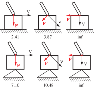
Figure 1: 2D examples of HFVC and their corresponding crashing indexes. The robot execute 2D HFVC, with 1D force control and 1D velocity control.

IV-B Problem Formulation

The task of hybrid servoing is to solve for:

1. the dimensions of force-controlled actions and velocity-controlled actions, $n_{af}$ and $n_{av}$, and

2. the directions to do force control and velocity control, described by the matrix $T$, and

3. the magnitude of force/velocity actions: $\eta_{af}$ and $w_{av}$,

so as to minimize the crashing index (9) subject to the following constraints:

• Any $v$ under the robot action shall satisfy the goal constraint (2);

• Any $f$ under the robot action shall satisfy the guard conditions (4).

We use the word ‘any’ because a HFVC usually cannot uniquely determine $v$ and $f$.

V APPROACH

In this section, we use the notation ${\mathbb{NULL}}(\cdot)$ and ${\mathbb{ROW}}(\cdot)$ to denote the null space and row space of the argument, respectively; use ${\rm{Null}}(\cdot)$ and ${\rm{Row}}(\cdot)$ to denote a matrix whose rows form an orthonormal basis of ${\mathbb{NULL}}(\cdot)$ and ${\mathbb{ROW}}(\cdot)$, respectively. We use ${\rm rows}(\cdot)$ to denote the number of rows in the argument.

Before introducing our algorithm, we need to make some observations about the nature of the problem. Since the feasible velocity $v$ under a HFVC may not be unique, the proper statement of the goal constraint is:

$$Gv=b_{G},\ \ \forall v\in\{v\ |\ Jv=0,Cv=b_{C}\},$$ (10)

i.e. we need to ensure all possible solutions satisfy the goal. This is an inclusion relationship between the solution sets of two linear equations, which is equivalent to:

1. The null space of $G$ contains the null space of $\left[\begin{array}[]{c}J\\ C\end{array}\right]$;

2. There exists a common special solution: $\exists v^{*}:Gv^{*}=b_{G},Jv^{*}=0,Cv^{*}=b_{C}$.

We call them the Goal-Inclusion conditions and will refer to them repeatedly. Condition 1) is equivalent to

$${\mathbb{NULL}}(\left[\begin{array}[]{c}J\\ C\end{array}\right])\subseteq{\mathbb{NULL}}(\left[\begin{array}[]{c}J\\ G\end{array}\right]),$$ (11)

which further implies

$${\rm rank}(\left[\begin{array}[]{c}J\\ C\end{array}\right])\geq{\rm rank}(\left[\begin{array}[]{c}J\\ G\end{array}\right]).$$ (12)

Due to the orthogonal complement relation between the row and null space of a matrix, the null space inclusion (11) can be reformulated as a reverse row space inclusion:

$${\rm rank}\left(\left[\begin{array}[]{c}J\\ C\end{array}\right]\right)={\rm rank}\left(\left[\begin{array}[]{c}J\\ C\\ G\end{array}\right]\right).$$ (13)

Our algorithm involves three steps. First, we derive the control axis directions to satisfy the Goal-Inclusion condition 1) while optimizing conditioning. Second, we compute the velocity control magnitudes to satisfy the Goal-Inclusion condition 2). Finally, we solve for the force control magnitudes to satisfy the guard conditions.

V-A Pick Control Axes to Optimize Conditioning

The information of the control axes ($n_{av},n_{af}$, and $T$) is contained in the velocity control coefficient matrix $C$ (5): $C$ has $n_{av}$ rows; $C$ and its orthogonal complement forms $T$.

First thing we need to know about the velocity control is its dimension. We can compute the instantaneous directions that the system can move without conflicting the contact constraints by computing the null space $U$ of contact Jacobian:

$$U={\rm Null}(J).$$ (14)

The last $n_{a}$ columns of $U$, i.e. the actuated part, indicate the directions in which the robot can move freely. It is a linear space, a basis of which can be computed as:

$$\bar{U}={\rm Row}(US_{a}),$$ (15)

where $S_{a}\in\mathbb{R}^{n\times n}$ is a selection matrix with only ones on the last $n_{a}$ diagonal entries. Any linear combinations of rows of $\bar{U}$ corresponds to a vector in ${\mathbb{NULL}}(J)$ and is thus a free robot motion direction. The dimensionality of $\bar{U}$ indicates the maximum dimension of velocity control we can apply:

$$n_{av}\leq{\rm rows}(\bar{U})$$ (16)

On the other hand, (12) suggests the minimum dimension of velocity control required to satisfy the goal (2):

$$n_{av}\geq{\rm rank}(\left[\begin{array}[]{c}J\\ G\end{array}\right])-{\rm rank}(J).$$ (17)

Combining (16) and (17), we have a necessary condition for the feasibility of the problem:

$${\rm rows}(\bar{U})\geq{\rm rank}(\left[\begin{array}[]{c}J\\ G\end{array}\right])-{\rm rank}(J).$$ (18)

If equation (18) is not satisfied, the problem has an infeasible goal. Otherwise, we can choose the dimension of velocity control within (16)-(17). Sometimes we want more velocity control so as to increase disturbance rejection ability [12]; sometimes we want less velocity control to have more compliance in the system [14]. We solve both situations and leave this choice to the user.

If the maximal velocity control is needed, we can simply do velocity control in all directions in $\bar{U}$:

$$n_{av}={\rm rows}(\bar{U}),$$ (19)

$$C=\bar{U}.$$ (20)

Then we check equation (13) to see if the problem is feasible. Otherwise, if the minimal velocity control is desired, we take

$$n_{av}={\rm rank}(\left[\begin{array}[]{c}J\\ G\end{array}\right])-{\rm rank}(J)$$ (21)

Then the $n_{av}$ rows of velocity controls are linear combinations of rows of $\bar{U}$:

$$C=K\bar{U},$$ (22)

where $K\in\mathbb{R}^{n_{av}\times{\rm rows}(\bar{U})}$. We compute $K$ using the null space form of Goal-Inclusion condition 1), which implies

$$C{\rm Null}(\left[\begin{array}[]{c}J\\ G\end{array}\right])=K\bar{U}{\rm Null}(\left[\begin{array}[]{c}J\\ G\end{array}\right])=0.$$ (23)

Then $K$ is an orthonormal basis of a null space:

$$K={\rm Null}^{T}\left({\rm Null}^{T}(\left[\begin{array}[]{c}J\\ G\end{array}\right])\bar{U}^{T}\right).$$ (24)

The problem is feasible if $K$ has enough rows:

$${\rm rows}(K)\geq n_{av}.$$ (25)

If this is true, we keep the first $n_{av}$ rows of $K$ and recover $C$ from equation (22). The $C$ obtained this way has orthonormal rows, since it is the product of two orthonormal matrices.

Note that equation (20) and (22) compute the velocity control direction $C$ in a closed form without explicitly optimize the crashing index (9), however, they do find optimal solutions. As shown in our numerical experiments, equation (22) always finds the solution with the minimal crashing index; equation (20) also always achieves the minimal crashing index among solutions with the same dimensionality.

After obtaining the velocity-controlled direction $C$, we compute the force-controlled direction as its orthogonal complement to make the velocity and force controls reciprocal. Denote the last $n_{a}$ columns of $C$ as $R_{C}$, we can expand it into a full rank $R_{a}$:

$$\begin{array}[]{rl}n_{af}&=n_{a}-n_{av}.\end{array}$$ (26)

$${R_{a}}=\left[{\begin{array}[]{*{20}{c}}{{\rm Null}{{({R_{C}})}^{T}}}\\ {{R_{C}}}\end{array}}\right].$$ (27)

Then we have $T=\rm{diag}(I_{u},R_{a})$.

We summarize the procedure in line 1 to line 1 in algorithm 1. Note that the method avoids the non-convex optimization in [14].

V-B Solve for Velocity Control Magnitudes

Next, we use Goal-Inclusion condition 2) to compute $b_{C}$. Compute a special solution $v^{*}$ from

$$\left[\begin{array}[]{c}J\\ G\end{array}\right]v^{*}=\left[\begin{array}[]{c}0\\ b_{G}\end{array}\right]$$ (28)

Such $v^{*}$ must exist, otherwise the goal itself is infeasible. Use it to compute the velocity control magnitude:

$$w_{av}=b_{C}=Cv^{*}$$ (29)

This choice of $b_{C}$ satisfies condition 2).

Input: Contact Jacobian $J$, Goal description $G,b_{G}$

Input: Guard condition,

Output: HFVC ($n_{af},n_{av},R_{a},w_{av},\eta_{af}$)

// Solve for velocity control

1 Compute free motion space $U$ under constraint;

2 Compute free robot motion space $\bar{U}$ (15) ;

3 Check necessary feasibility condition (18). ;

4 if Maximal velocity control dimension then

5       Take $\bar{U}$ as velocity-controlled directions (19)(20) ;

6       Check goal feasibility using (13);

7      

8 else

9       Compute the minimal dimension of $C$ from (21) ;

10       Solve for the coefficient matrix $K$ from (24) ;

11       Check goal feasibility using (25) ;

12       Compute the velocity control $C$ from (22);

13      

14 Complete control axes information using (26)-(27). ;

15 Compute the velocity control magnitude (29) using a special solution to (28). ;

// Solve for Force control

16 Compute the force control magnitude $\eta_{af}$ by solving the QP defined in Section V-C.;

Algorithm 1 Optimally-Conditioned Hybrid Servoing

V-C Solve for Force Control Magnitudes

At this point we already know the dimensionality and directions of force control. The only remaining unknown variable in a HFVC is the value of the force control magnitude $\eta_{af}$. we find a solution by minimizing the magnitude of force variables:

$$\min_{\lambda,\eta}\lambda^{T}\lambda+\eta_{a}^{T}\eta_{a}$$ (30)

subject to the Newton’s Second Law (3) and the guard conditions (4), which takes the form of a Quadratic Programming. This is a simplified version of the force magnitude computation in [14] and it is slightly more efficient.

V-D Discussion

An important advantage of this algorithm over the previous work [14] is its ability to handle underactuated system.

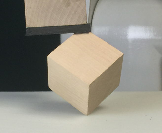
Figure 2: An underactuated example.

An example is a cube with one corner sticking on the ground and one corner sticking on the robot finger (Figure 2): the robot has no control over the rotation of the cube about the line between the two contact points. Still, a control problem on this object may still be feasible, e.g. if the goal is to lift the center of mass of the object. Condition (13) tells us whether this is the case or not.

VI Evaluation

VI-A Implementation

In this section, we evaluate the performance of the OCHS algorithm in randomly generated manipulation problems. We implement OCHS in Matlab and test it on a desktop with an i7-9700k CPU clocked at 4.7GHz.

VI-B Test Problems

We consider a rigid object with one to three environmental contacts and one to three rigid body fingers. Each rigid body has three DOFs in planar problems, or six DOFs in 3D problems. The settings are listed in Table I, where ‘f’ denotes a fixed (sticking) contact point, ‘s’ denotes a sliding contact point. Each environment contact point can be sliding or sticking; finger contacts are all sticking.

TABLE I: Types of Randomly Generated Test Problems

	Environment Contacts		Hand Contacts
	# Contact Points	Contact Modes	# Contacts per finger	# Fingers
Planar	1	f,s	1,2	1
	2	ss	1,2	1
3D	1	f,s	1,2,3	1,2,3
	2	ff,fs,ss	1,2,3	1,2,3
	3	ffs,fss,sss	1,2,3	1,2,3

TABLE II: Test results - Min Velocity Control Dimension

Planar (6 DOF)		OCHS	OCHS(M)	HS3	HS10
# of Problems	Total	6000
	Solved	5985	5981	5974	5977
Average Crashing Index		15.5	18.4	19.5	19.9
ill-conditioned solutions		15	19	26	23
Velocity Time(ms)	Average	0.14	0.14	1.74	5.32
	Worst	0.63	0.46	2.73	7.40
Force Time (ms)	Average	0.99	0.94	1.28	1.33
	Worst	2.21	2.44	2.09	3.34

3D, (12 to 24 DOF)		OCHS	OCHS(M)	HS3	HS10
# of Problems	Total	72000
	Solved	67506	67399	65950	65952
Average Crashing Index		3.98	13.8	5.20	4.68
ill-conditioned solutions		22	136	50	48
Velocity Time(ms)	Average	0.28	0.28	1.96	5.70
	Worst	0.85	0.77	3.82	10.7
Force Time (ms)	Average	1.09	1.04	1.57	1.61
	Worst	3.03	3.13	12.3	11.8

TABLE III: Test results - Max Velocity Control Dimension

		OCHS	OCHS(M)	HS3	HS10
# of Problems	Total	30000
	Solved	27372	27372	22939	22951
Average Crashing Index		8.34	8.34	14.0	12.9
ill-conditioned solutions		55	55	37	31
Velocity Time(ms)	Average	0.17	0.17	2.35	7.25
	Worst	0.54	0.45	3.99	28.39
Force Time (ms)	Average	1.04	0.98	1.39	1.44
	Worst	2.39	2.18	3.76	3.62

We randomly sample 1000 set of contact point locations and normals for each contact mode setting, making a total of 6000 planar and 72,000 3D test problems. The goal constraint is sampled randomly for each problem.

The results are summarized in Table III and III, the difference is that in Table III we give the goal (2) the maximum possible dimension, so all algorithms must select the maximum velocity control dimension. OCHS is our algorithm with minimal velocity control, OCHS(M) denotes our algorithm with maximal velocity control. As a comparison, we also show the performance of the original hybrid servoing algorithm [14]. HS3 uses three initial guesses and has a good computation speed; HS10 uses ten initial guesses to search the problem excessively. Both run each initial guess for 50 iterations.

VI-C Results

In all tests, OCHS consistently finds solutions with better crashing indexes than HS3 and HS10, achieves lower average crashing index and fewer ill-conditioned solutions. OCHS(M) has a larger crashing index in Table III because it applies more dimensions of control. When all algorithms selects the same dimension of velocity control, OCHS(M) also always achieves better crashing indexes than HS3 and HS10 on every problem.

Both OCHS and OCHS(M) are notably faster than HS3 and HS10. The velocity part of OCHS shows 7 to 13 times speedup comparing with HS3, 20 to 40 times speedup comparing with HS10. The force part of OCHS has a mild speed up of 35% due to a simpler problem formulation with less variables.

VII EXPERIMENTS

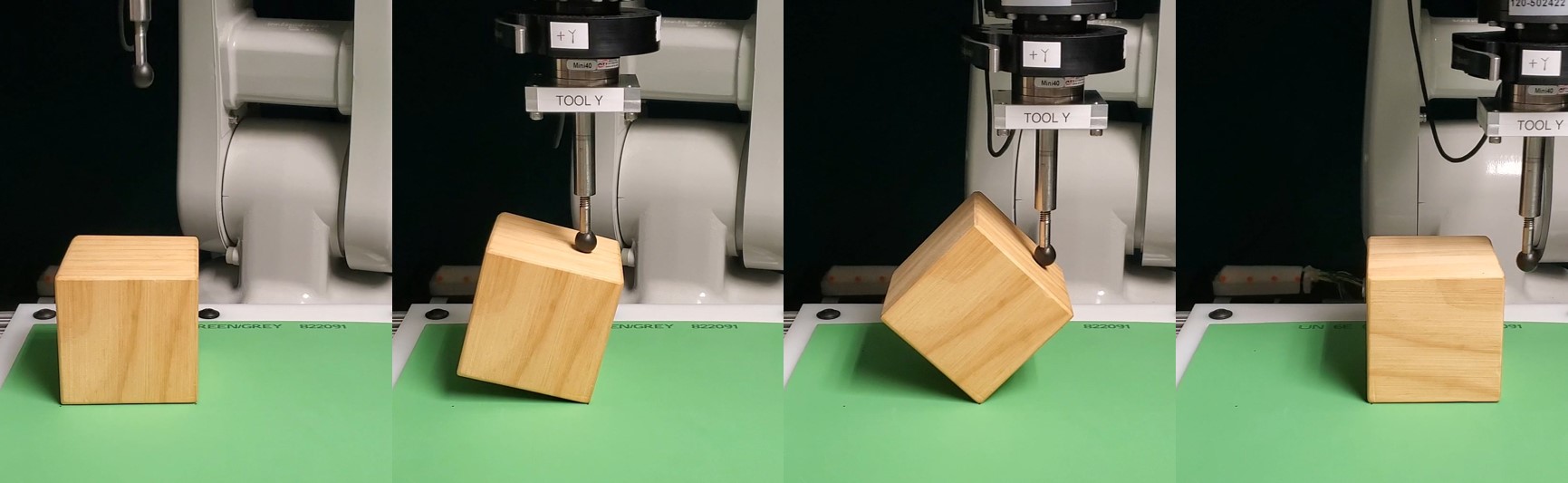
Figure 3: Robot flipping a block with one fingertip. The experiment runs 100 times with all successes.

We test the quality of our algorithm in several experiments. We implemented hybrid force-velocity control on a position-controlled ABB IRB 120 industrial robot with a wrist-mounted ATI Mini-40 force-torque sensor. In all experiments, we run OCHS off-line on a given motion plan to obtain a trajectory of HFVC, though the computation speed of OCHS supports feedback control at hundreds of Hz. In online execution, HFVC control loop is clocked at 200Hz. The lowest communication rate between the computer and the robot position controller is 250Hz with 25ms latency.

To compare with our previous work, we redo the block tilting experiment [14] with the same setup, as shown in Figure 3. The block is a wooden cube with length 75mm. We place a 1.5mm rubber sheet on the table to increase friction. The robot hand is the same rubber ball as before. In our previous work, we perform block tilting 50 times and obtained 47 successes. With OCHS, we obtain a hundred consecutive successes at 50% higher robot velocity . The result demonstrate the ability of our algorithm to consistently produce solutions with good quality.

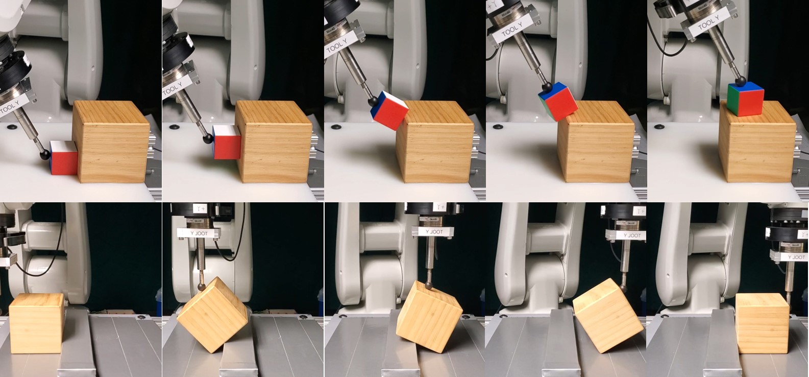
Figure 4: Two shared grasping tasks executed with OCHS. Top: moving an object up a stair. Bottom: transporting an object over an obstacle.

OCHS can be used in shared grasping [12] to compute the control axes and velocity control. We use OCHS as a robust tracking controller to execute several shared grasping with motion plans computed using [6], as shown in Figure 4.

VIII CONCLUSION

In this work, we provide an algorithm to compute a hybrid force-velocity control for manipulation under contact constraints. Our algorithm finds the solution that brings the best kinematic conditioning of the manipulation system. We demonstrate that our algorithm reliably and quickly finds the best solutions among all comparisons in extensive tests and experiments.

The algorithm itself can serve as a robust tracking controller to execute a pre-computed motion plan. It is also a building block for the more comprehensive contact stability analysis [12]. Due to our algorithm’s computational efficiency, it also has the potential to be incorporated into a planning framework for robust manipulation planning.

References

- [1] Jorge Angeles and Carlos S López-Cajún. Kinematic isotropy and the conditioning index of serial robotic manipulators. The International Journal of Robotics Research, 11(6):560–571, 1992.
- [2] Jorge Angeles, Farzam Ranjbaran, and Rajnikant V Patel. On the design of the kinematic structure of seven-axes redundant manipulators for maximum conditioning. In Proceedings 1992 IEEE International Conference on Robotics and Automation, pages 494–495. IEEE Computer Society, 1992.
- [3] Bernard Brogliato, S-I Niculescu, and Pascal Orhant. On the control of finite-dimensional mechanical systems with unilateral constraints. IEEE Transactions on Automatic Control, 42(2):200–215, 1997.
- [4] Thomas Buschmann, Sebastian Lohmeier, and Heinz Ulbrich. Biped walking control based on hybrid position/force control. pages 3019–3024, 2009.
- [5] Nikhil Chavan-Dafle and Alberto Rodriguez. Prehensile pushing: In-hand manipulation with push-primitives. In 2015 IEEE/RSJ International Conference on Intelligent Robots and Systems, pages 6215–6222, 2015.
- [6] Xianyi Cheng, Eric Huang, Yifan Hou, and Matthew T Mason. Contact mode guided sampling-based planningfor quasistatic dexterous manipulation in 2d. Under Review, 2020.
- [7] Joris De Schutter, Herman Bruyninckx, Wen-Hong Zhu, and Mark W Spong. Force control: a bird’s eye view. In Control Problems in Robotics and Automation, pages 1–17. Springer, 1998.
- [8] Niels Dehio, Joshua Smith, Dennis Leroy Wigand, Guiyang Xin, Hsiu-Chin Lin, Jochen J Steil, and Michael Mistry. Modeling and control of multi-arm and multi-leg robots: Compensating for object dynamics during grasping. In 2018 IEEE International Conference on Robotics and Automation (ICRA), pages 294–301. IEEE, 2018.
- [9] Steven Eppinger and W Seering. Introduction to dynamic models for robot force control. IEEE Control Systems Magazine, 7(2):48–52, 1987.
- [10] Yasutaka Fujimoto and Atsuo Kawamura. Proposal of biped walking control based on robust hybrid position/force control. In Proceedings of IEEE International Conference on Robotics and Automation, volume 3, pages 2724–2730. IEEE, 1996.
- [11] Neville Hogan. Impedance control: An approach to manipulation: Part ii—implementation. Journal of dynamic systems, measurement, and control, 107(1):8–16, 1985.
- [12] Yifan Hou, Zhenzhong Jia, and Matthew T Mason. Manipulation with shared grasping. Robotics: Science and Systems, 2020.
- [13] Yifan Hou and Matthew T Mason. Criteria for maintaining desired contacts for quasi-static systems. In Proceedings of IEEE/RSJ International Conference on Intelligent Robots and Systems. IEEE, November 2019.
- [14] Yifan Hou and Matthew T Mason. Robust execution of contact-rich motion plans by hybrid force-velocity control. In International Conference on Robotics and Automation (ICRA) 2019. IEEE Robotics and Automation Society (RAS), May 2019.
- [15] Hiroshi Ishikawa, Chihiro Sawada, K Kawasa, and Masayuki Takata. Stable compliance control and its implementation for a 6 dof manipulator. In Proceedings, 1989 International Conference on Robotics and Automation, pages 98–103. IEEE, 1989.
- [16] H Kazerooni, BJ Waibel, and S Kim. On the stability of robot compliant motion control: theory and experiments. Journal of Dynamic Systems, Measurement, and Control, 112(3):417–426, 1990.
- [17] Oussama Khatib. A unified approach for motion and force control of robot manipulators: The operational space formulation. IEEE Journal on Robotics and Automation, 3(1):43–53, 1987.
- [18] António Lopes and Fernando Almeida. A force–impedance controlled industrial robot using an active robotic auxiliary device. Robotics and Computer-Integrated Manufacturing, 24(3):299–309, 2008.
- [19] J. Maples and J. Becker. Experiments in force control of robotic manipulators. In Proceedings. 1986 IEEE International Conference on Robotics and Automation, volume 3, pages 695–702, Apr 1986.
- [20] Matthew T Mason. Compliance and force control for computer controlled manipulators. IEEE Transactions on Systems, Man, and Cybernetics, 11(6):418–432, 1981.
- [21] N Harris McClamroch and Danwei Wang. Feedback stabilization and tracking of constrained robots. IEEE Transactions on Automatic Control, 33(5):419–426, 1988.
- [22] James K Mills and David M Lokhorst. Control of robotic manipulators during general task execution: A discontinuous control approach. The International Journal of Robotics Research, 12(2):146–163, 1993.
- [23] Richard M Murray, Zexiang Li, and S. Shankar Sastry. A Mathematical Introduction to Robotic Manipulation. CRC Press, Inc., USA, 1st edition, 1994.
- [24] Fusaomi Nagata, Tetsuo Hase, Zenku Haga, Masaaki Omoto, and Keigo Watanabe. Cad/cam-based position/force controller for a mold polishing robot. Mechatronics, 17(4-5):207–216, 2007.
- [25] Hyeonjun Park, Jaeheung Park, Dong-Hyuk Lee, Jae-Han Park, Moon-Hong Baeg, and Ji-Hun Bae. Compliance-based robotic peg-in-hole assembly strategy without force feedback. IEEE Transactions on Industrial Electronics, 64(8):6299–6309, 2017.
- [26] Marc H Raibert and John J Craig. Hybrid position/force control of manipulators. Journal of Dynamic Systems, Measurement, and Control, 103(2):126–133, 1981.
- [27] J Kenneth Salisbury. Active stiffness control of a manipulator in cartesian coordinates. In Decision and Control including the Symposium on Adaptive Processes, 1980 19th IEEE Conference on, volume 19, pages 95–100. IEEE, 1980.
- [28] J Kenneth Salisbury and John J Craig. Articulated hands: Force control and kinematic issues. The International journal of Robotics research, 1(1):4–17, 1982.
- [29] G. W. Stewart. Collinearity and least squares regression. Statistical Science, 2(1):68–84, 1987.
- [30] Masaru Uchiyama and Pierre Dauchez. A symmetric hybrid position/force control scheme for the coordination of two robots. In Robotics and Automation, 1988. Proceedings., 1988 IEEE International Conference on, pages 350–356. IEEE, 1988.
- [31] Luigi Villani and Joris De Schutter. Force control. In Springer handbook of robotics, pages 161–185. Springer, 2008.
- [32] Richard Volpe and Pradeep Khosla. A theoretical and experimental investigation of impact control for manipulators. The International Journal of Robotics Research, 12(4):351–365, 1993.
- [33] Harry West and Haruhiko Asada. A method for the design of hybrid position/force controllers for manipulators constrained by contact with the environment. In Proceedings. 1985 IEEE International Conference on Robotics and Automation, volume 2, pages 251–259. IEEE, 1985.
- [34] Daniel E Whitney. Historical perspective and state of the art in robot force control. The International Journal of Robotics Research, 6(1):3–14, 1987.
- [35] Tsuneo Yoshikawa. Dynamic hybrid position/force control of robot manipulators–description of hand constraints and calculation of joint driving force. IEEE Journal on Robotics and Automation, 3(5):386–392, 1987.