Understanding the scaling of boson peak through insensitivity of elastic heterogeneity to bending rigidity in polymer glasses
Abstract
Amorphous materials exhibit peculiar mechanical and vibrational properties, including non-affine elastic responses and excess vibrational states, i.e., the so-called boson peak. For polymer glasses, these properties are considered to be affected by the bending rigidity of the constituent polymer chains. In our recent work [Tomoshige, et al., Sci. Rep. 9 19514 (2019)], we have revealed simple relationships between the variations of vibrational properties and the global elastic properties: the response of the boson peak scales only with that of the global shear modulus. This observation suggests that the spatial heterogeneity of the local shear modulus distribution is insensitive to changes in the bending rigidity. Here, we demonstrate the insensitivity of elastic heterogeneity by directly measuring the local shear modulus distribution. We also study transverse sound wave propagation, which is also shown to scale only with the global shear modulus. Through these analyses, we conclude that the bending rigidity does not alter the spatial heterogeneity of the local shear modulus distribution, which yields vibrational and acoustic properties that are controlled solely by the global shear modulus of a polymer glass.
I Introduction
Amorphous materials exhibit anomalous mechanical and vibrational properties that have been studied for many years by experimental, numerically, and theoretical methods. The vibrational and acoustical properties of such materials have been investigated in many experiments using neutron, light, and X-ray scattering, e.g., Refs. Monaco et al. (2006); Baldi et al. (2010); Chumakov et al. (2011); Yamamuro et al. (1996); Ramos et al. (2003); Monaco and Giordano (2009); Shibata et al. (2015); Kabeya et al. (2016); Mori et al. (2020). Using these methods, anomalies in vibrational and acoustic excitations have been detected, including excess vibrational states, the so-called boson peak (BP), and strong damping of sound wave propagation.
To explain these anomalous properties, the heterogeneous elasticity theory was proposed and developed by Schirmacher and co-workers Schirmacher (2006); Schirmacher et al. (2007); Köhler et al. (2013); Schirmacher et al. (2015) (see also Refs. Wyart (2010); DeGiuli et al. (2014) for the theory in the context of the jamming transition and Refs. Shimada et al. (2020, 2021); Shimada and De Giuli (2020) for very recent developments). It is now well-established that amorphous materials exhibit spatial heterogeneity in their local elastic modulus distributions, as supported by numerical simulations Tsamados et al. (2009); Makke et al. (2011); Mizuno et al. (2013a) and experiments Wagner et al. (2011); Hufnagel (2015). In the theory, elastic moduli heterogeneities are critical in describing anomalies in the vibrational, acoustic, and thermal properties. The theory notably predicts that the BP and the attenuation rate of sound are more significant when moduli distributions are more heterogeneous. This prediction has been tested and justified by numerical simulations Marruzzo et al. (2013a, b); Mizuno et al. (2013b, 2014, 2016); Shakerpoor et al. (2020); Kapteijns et al. (2021).
Anomalous behaviours in polymer glasses have also been reported through both experiments Niss et al. (2007); Hong et al. (2008); Caponi et al. (2011); Pérez-Castañeda et al. (2014); Terao et al. (2018); Zorn et al. (2018); Corezzi and Comez (2020) and numerical simulations Jain and de Pablo (2004); Schnell et al. (2011); Lappala et al. (2016); Ness et al. (2017); Milkus et al. (2018); Giuntoli and Leporini (2018). In polymer glasses, the bending rigidity of the constituent polymer chains is an important parameter. In our recent work Tomoshige et al. (2019), we studied the effects of the bending rigidity on the global elastic moduli (shear modulus and bulk modulus ) and the vibrational density of states (vDOS) using coarse-grained molecular dynamics (MD) simulations. We demonstrated that the variation of the BP simply follows that of global shear modulus through the Debye frequency . If this simple scaling behaviour is considered in terms of the heterogeneous elasticity theory, we obtain an important implication that the spatial heterogeneity in local modulus distributions is insensitive to changes in the bending rigidity.
In this study, we examine this correlation by directly measuring the degree of elastic heterogeneity with changes in the bending rigidity. We also study transverse acoustic excitations in the polymer glasses by calculating the dynamic structure factor and examine the connection among the sound velocity, attenuation rate, and the simple scaling behaviour of the BP. Thus, we comprehensively discuss that the effects of bending rigidity in polymer glasses on vibrational and acoustic excitations from the perspective of elastic heterogeneities.
II Simulation method
II.1 Simulation model
We performed MD simulations using the Kremer–Grest model Kremer and Grest (1990), which is a coarse-grained bead-spring model of the polymer chain. Each polymer chain comprises monomer beads of mass and diameter . We studied the case of chains of , such that the system contained monomer beads in total, in a three-dimensional cubic box of volume under periodic boundary conditions.
In the Kremer–Grest model, three types of inter-particle potentials are utilised. First, the Lennard-Jones (LJ) potential
| (1) |
acts between all pairs of monomer beads, where and denote the distance between two monomers and the energy scale of the LJ potential, respectively. The LJ potential is truncated at the cut-off distance of , where the potential and the force (the first derivative of the potential) are shifted to zero continuously Shimada et al. (2018).
Second, sequential monomer beads along the polymer chain are connected by a finitely extensible nonlinear elastic (FENE) potential:
| (2) |
where is the energy scale of the FENE potential, and is the maximum length of the FENE bond. Following Ref. Milkus et al. (2018), we employ the values of and .
Finally, the bending angle formed by three consecutive monomer beads along the polymer chain is controlled by
| (3) |
where is the associated bending energy. We set the stabilised angle as Milkus et al. (2018). In the present work, we utilise a wide range of values: , , , , , , , , and .
We performed the MD simulations using the Large-scale Atomic/Molecular Massively Parallel Simulator (LAMMPS) Plimpton (1995). Hereafter, the length, energy, and time are measured in units of , , and , respectively. The temperature is presented in units of , where is the Boltzmann constant. We first equilibrated the polymer melt system at a temperature and polymer bead number density . We then cooled the system down towards with a constant cooling rate of , under a fixed pressure of . Finally, the inherent structure at is generated using the steepest descent method. In our recent work Tomoshige et al. (2019), we reported the dependence of the glass transition temperature and the number density at zero temperature on .
II.2 Vibrational density of state and boson peak
The vDOS analysis was performed for the configuration at . By diagonalizing the Hessian matrix, we obtained the eigenvalues (, 2, , ), which provide the eigenfrequencies as . The vDOS is defined as
| (4) |
where three zero-frequency modes are omitted. The expression of the Hessian matrix of the polymeric system was given in Ref. Tomoshige et al. (2019). The Debye law predicts the vDOS as , where is the Debye level using the Debye frequency . Here, the transverse and longitudinal sound velocities, and , are given by the bulk modulus , shear modulus , and the mass density as and , respectively. The reduced vDOS thus characterises the excess vibrational modes exceeding the Debye prediction, i.e., the BP.
II.3 Global and local shear modulus
The global shear modulus and bulk modulus were evaluated from the stress-tensor response to the shear and volume deformations in the “quasi-static” way, respectively, applied to the inherent structure. For perfect crystalline solids, the mechanical equilibrium is maintained during affine deformation. However, the force balance is generally broken down for amorphous solids under applied affine deformations. Thus, further energy minimization causes additional non-affine deformation (relaxation) towards mechanical equilibrium. In other words, and are decomposed into and . Here, and denote the affine and non-affine components of elastic moduli, with and , respectively. Our recent work Tomoshige et al. (2019) also reported the dependence of and . In particular, we demonstrated that the bulk modulus is much larger than the shear modulus , and thus the shear modulus has important effects on the low-frequency vibrational properties of the polymeric system.
In this study, we further study the local shear modulus. Specifically, we measure the spatial distribution of the local shear modulus , by using the numerical procedure of “affine strain approach”, given in Ref. Mizuno et al. (2013a). Note that the analysis completely neglects anharmonic effects and provide zero-temperature limit values of elastic heterogeneities. Briefly, we divided the system into 77 cubic cells and monitored the local shear stress as a function of the applied shear strain in each local cell. The linear dimension of the cell is approximately . Here, the local strain of the small cell is assumed to be given by the global strain applied to the system. The local shear modulus of cell was measured as the slope of the local shear stress versus the shear strain. The expression of the local modulus was also given in Ref. Mizuno et al. (2013a). Finally, we collected the values for all the cells to calculate the probability distribution of the local shear modulus . Remark that the average and standard deviation of the local shear modulus distribution is insensitive to the cell size Mizuno et al. (2013a).
II.4 Transverse acoustic excitation
The transverse acoustic excitation can be characterised by the (transverse) dynamic structure factor as a function of the wave vector and frequency Marruzzo et al. (2013a); Mizuno et al. (2014); Monaco and Mossa (2009); Beltukov et al. (2016):
| (6) |
where , ‘’ indicates complex conjugation, and denotes the ensemble average over the initial time and angular components of . Here, the transverse current is expressed by:
| (7) |
where , and and represent the position and velocity, respectively, of the monomer bead . In general, the dynamic structure factor exhibits two kinds of peaks: the Rayleigh (elastic) peak and the Brillouin (inelastic) peak. The Rayleigh peak is located at and is related to the thermal diffusion, while the Brillouin peak is related to the (transverse) sound-wave propagation.
The Brillouin peak in can be fitted by the damped harmonic oscillator function Marruzzo et al. (2013a); Mizuno et al. (2014); Monaco and Mossa (2009); Beltukov et al. (2016),
| (8) |
which provides information about the propagation frequency and the attenuation rate as functions of the wave number . The sound velocity is then given by . Note that the sound velocity converges to the macroscopic value in the long-wavelength limit of . We numerically calculated the dynamic structure factor [Eq. (6)] of the inherent structure for each bending energy from to . Note that the thermal fluctuations are imposed at very low temperature , which is small enough that the derived values are consistent with the zero-temperature limit values. The values of and were then extracted using Eq. (8).
III Results and Discussion
III.1 Scaling of boson peak by the Debye frequency and Debye level
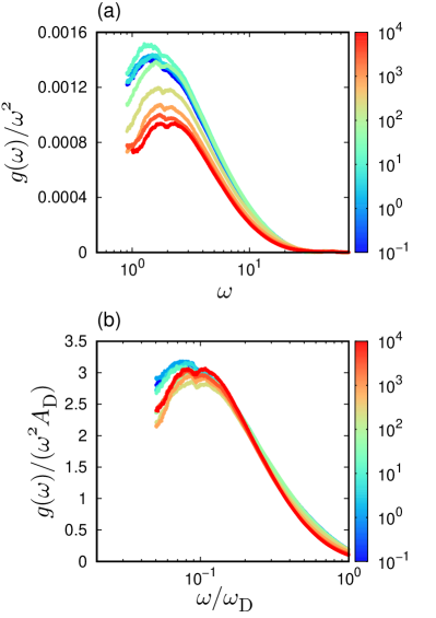
Figure 1(a) plots the reduced vDOS , showing the BP beyond the Debey level for each . The BP frequency is located at , but it slightly shifts to the higher frequency with increasing the bending rigidity. In addition, the peak height of gradually decreases when is increased. Figure 1(b) shows the reduced vDOS scaled by the Debye level as a function of the frequency scaled by the Debye frequency . This demonstrates the scaling of the BP by the Debye frequency and Debye level for various bendig rigidities of the polymer chain. Note that the scaling property of the BP is also shown for shorter polymer chain with the length in our previous paper Tomoshige et al. (2019).
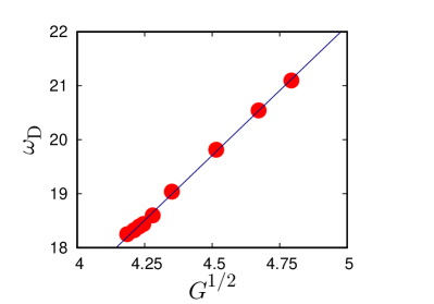
III.2 Debye frequency and global shear modulus
We next examine the relationship between the Debye frequency and the shear modulus , which is plotted in Fig. 2. As demonstrated in Ref. Tomoshige et al. (2019), the bulk modulus is approximately three to four times larger than the shear modulus . Thus the term becomes negligible, and the Debye frequency can be approximated as
| (9) |
which is mainly governed by the shear modulus . Figure 2 directly demonstrates the relationship of with changes in . The density is also changed by changing , but the effect of density on is close to negligible Tomoshige et al. (2019).
III.3 Local shear modulus distribution
As demonstrated in Fig. 1, the reduced vDOS in the BP frequency regime was well scaled by using the Debye frequency and Debye level This suggests that the frequency and intensity of BP are controlled only by the global sear modulus . In particular, we obtain the relationship of . According to the heterogeneous elasticity theory Schirmacher (2006); Schirmacher et al. (2007); Köhler et al. (2013); Schirmacher et al. (2015), this observation implies that the degree of the shear modulus heterogeneity is invariant with changes in the bending energy : this implication is confirmed below.
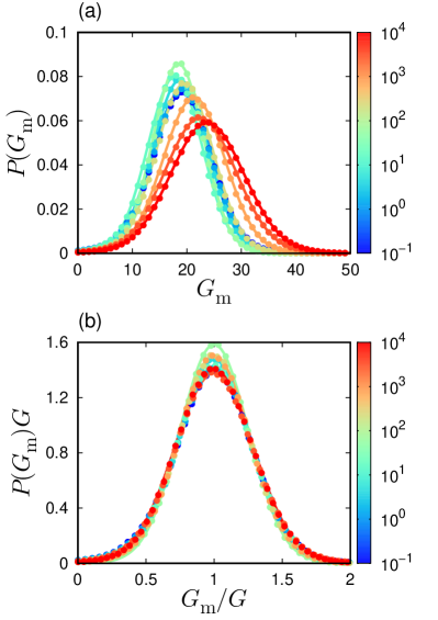
We plot the probability distribution of the local shear modulus in Fig. 3(a); this plot follows the Gaussian form of Eq. (5). Figure 3(b) then plots the scaled distribution as a function of the scaled local shear modulus , demonstrating the data of versus nicely collapse for different values of . Because we can transform (Gaussian form) to
| (10) |
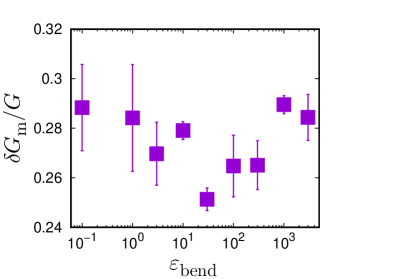
this collapse indicates that the scaled standard deviation remains unchanged for different values. This is verified by direct demonstration in Fig. 4, where is plotted explicitly as a function of . Therefore, we can conclude that the bending rigidity of the polymer chain does not alter the degree of the shear modulus heterogeneity. This conclusion justifies the theoretical prediction Schirmacher (2006); Schirmacher et al. (2007); Köhler et al. (2013); Schirmacher et al. (2015) that vibrational excitations including the BP are controlled only by the global elastic modulus under the condition of constant heterogeneities in the moduli distributions.
III.4 Transverse acoustic excitation and its link with boson peak
We finally study the transverse acoustic excitation in the frequency regime including the BP. The generalised Debye model Marruzzo et al. (2013a); Mizuno and Ikeda (2018) yields the reduced vDOS in terms of the propagation frequency and the attenuation rate , as follows:
| (11) |
with Debye wavenumber . This form can be scaled by and as:
| (12) |
Thus, the collapse of the reduced vDOSs for different values of indicates that and are both independent of the bending energy .
In addition, Eq. (8), which is the damped harmonic oscillator function for the dynamic structure factor , can be scaled by the Debye frequency :
| (13) |
which indicates that is simply scaled by , when and are independent of . Below we show that these properties of transverse acoustic excitations are true.
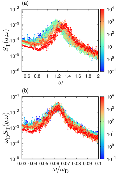
Figure 5(a) shows the for different values of . The wave number is set to its lowest value , which ranges from (for ) to (for ). The frequency of the Brillouin peak shifts to higher values with increasing . We then plot versus in Fig. 5(b). It is evident that our calculations of are in accordance with the predicted scaling description of Eq. (13).
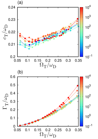
We also show the sound velocity and attenuation rate as functions of the frequency in Fig. 6. As expected from the scaling property of , the data of and collapse for different values of , although small deviations are detected. These collapses are also consistent with the prediction from Eq. (12) and are explained in terms of the shear modulus heterogeneity. The collapses break down in the high frequency regime above the BP frequency, . Because the generalized Debye model does not hold above the BP frequency Marruzzo et al. (2013a); Mizuno and Ikeda (2018), this deviation is not unexpected.
IV Conclusion
In conclusion, we have numerically studied elastic heterogeneities and acoustic excitations in polymer glasses, with particular attention to the effects of the bending rigidity of the constituent polymer chains. Our main finding is that the degree of heterogeneity in the local shear modulus distribution is insensitive to changes in the bending rigidity. According to the heterogeneous elasticity theory, for unchanging elastic heterogeneities, the vibrational and acoustic properties of amorphous materials are controlled only by global elastic moduli. Consistent with this theoretical prediction, we demonstrated that the BP and properties of the transverse acoustic excitations are both simply scaled only by the global shear modulus. The present work therefore clarified remarkably simple material property relationships in polymer glasses. These originate from the invariance of the local elastic heterogeneities over an extremely wide range of bending rigidity values for polymer chains. Our results also provide good demonstrations that verify the heterogeneous elasticity theory Schirmacher (2006); Schirmacher et al. (2007); Köhler et al. (2013); Schirmacher et al. (2015), which is among the central theories used to describe the mechanical and vibrational properties of amorphous materials.
We note that effects of polymerization on vibrational properties can be scaled by global elastic moduli Caponi et al. (2011); Corezzi and Comez (2020). On the contrary, some experiments demonstrate that the pressure-induced shift of BP cannot be explained by the global elastic moduli Niss et al. (2007); Hong et al. (2008). From these observations, we speculate that the polymerization effect is insensitive to the elastic heterogeneities as is the bending rigidity, whereas the heterogeneities would be altered by the densification. Furthermore, recent MD simulations revealed antiplasticizer additives significantly modify the local elastic constant distribution in glass-forming polymer liquids Riggleman et al. (2010). It could be interesting to study how boson peak properties change with evolution of elastic heterogeneities during the antiplasticization process.
At the end of this paper, we would discuss the relationship between the structural relaxation time and the elastic properties. Remarkably, numerical work Larini et al. (2008) has proposed and demonstrated a scaling relationship between the structural relaxation time and the Debye–Waller factor for many types of glass-forming systems, including polymer glasses, as (where and are constants). Because the Debye–Waller factor in the harmonic approximation limit is estimated as (where is applied) Shiba et al. (2016), we obtain
| (14) |
where , , , and are constants. This is the idea of the shoving model Dyre (1998, 2006), which characterises the activation energy in terms of the global shear modulus . Interestingly, Eq. (14) has been well demonstrated for polymer glasses by MD simulations, where the plateau modulus of the stress correlation function was effectively utilized as the shear modulus Puosi and Leporini (2012). Our results suggest an important condition under which Eq. (14) holds. When the spatial heterogeneity in the local shear modulus distribution is unchanged, the excess vibrational excitations, i.e., the BP, are controlled only by the global shear modulus, indicating that the structural relaxation time is also controlled solely by the global shear modulus.
Acknowledgements.
This work was supported by JSPS KAKENHI Grant Numbers: JP19K14670 (H.M.), JP20H01868 (H.M.), JP18H01188 (K.K.), JP20H05221 (K.K.), and JP19H04206 (N.M.). This work was also partially supported by the Asahi Glass Foundation and by the Fugaku Supercomputing Project and the Elements Strategy Initiative for Catalysts and Batteries (No. JPMXP0112101003) from the Ministry of Education, Culture, Sports, Science, and Technology. The numerical calculations were performed at Research Center of Computational Science, Okazaki Research Facilities, National Institutes of Natural Sciences, Japan.References
- Monaco et al. (2006) A. Monaco, A. I. Chumakov, G. Monaco, W. A. Crichton, A. Meyer, L. Comez, D. Fioretto, J. Korecki, and R. Rüffer, Phys. Rev. Lett. 97, 135501 (2006).
- Baldi et al. (2010) G. Baldi, V. M. Giordano, G. Monaco, and B. Ruta, Phys. Rev. Lett. 104, 195501 (2010).
- Chumakov et al. (2011) A. I. Chumakov, G. Monaco, A. Monaco, W. A. Crichton, A. Bosak, R. Rüffer, A. Meyer, F. Kargl, L. Comez, D. Fioretto, H. Giefers, S. Roitsch, G. Wortmann, M. H. Manghnani, A. Hushur, Q. Williams, J. Balogh, K. Parliński, P. Jochym, and P. Piekarz, Phys. Rev. Lett. 106, 225501 (2011).
- Yamamuro et al. (1996) O. Yamamuro, T. Matsuo, K. Takeda, T. Kanaya, T. Kawaguchi, and K. Kaji, J. Chem. Phys. 105, 732 (1996).
- Ramos et al. (2003) M. A. Ramos, C. Talón, R. J. Jiménez-Riobóo, and S. Vieira, J. Phys.: Condens. Matter 15, S1007 (2003).
- Monaco and Giordano (2009) G. Monaco and V. M. Giordano, Proc. Natl. Acad. Sci. U.S.A. 106, 3659 (2009).
- Shibata et al. (2015) T. Shibata, T. Mori, and S. Kojima, Spectrochim. Acta A 150, 207 (2015).
- Kabeya et al. (2016) M. Kabeya, T. Mori, Y. Fujii, A. Koreeda, B. W. Lee, J.-H. Ko, and S. Kojima, Phys. Rev. B 94, 224204 (2016).
- Mori et al. (2020) T. Mori, Y. Jiang, Y. Fujii, S. Kitani, H. Mizuno, A. Koreeda, L. Motoji, H. Tokoro, K. Shiraki, Y. Yamamoto, and S. Kojima, Phys. Rev. E 102, 022502 (2020).
- Schirmacher (2006) W. Schirmacher, EPL 73, 892 (2006).
- Schirmacher et al. (2007) W. Schirmacher, G. Ruocco, and T. Scopigno, Phys. Rev. Lett. 98, 025501 (2007).
- Köhler et al. (2013) S. Köhler, G. Ruocco, and W. Schirmacher, Phys. Rev. B 88, 064203 (2013).
- Schirmacher et al. (2015) W. Schirmacher, T. Scopigno, and G. Ruocco, J. Non-Cryst. Solids 407, 133 (2015).
- Wyart (2010) M. Wyart, EPL 89, 64001 (2010).
- DeGiuli et al. (2014) E. DeGiuli, A. Laversanne-Finot, G. Düring, E. Lerner, and M. Wyart, Soft Matter 10, 5628 (2014).
- Shimada et al. (2020) M. Shimada, H. Mizuno, and A. Ikeda, Soft Matter 16, 7279 (2020).
- Shimada et al. (2021) M. Shimada, H. Mizuno, and A. Ikeda, Soft Matter 17, 346 (2021).
- Shimada and De Giuli (2020) M. Shimada and E. De Giuli, arXiv (2020), 2008.11896 .
- Tsamados et al. (2009) M. Tsamados, A. Tanguy, C. Goldenberg, and J.-L. Barrat, Phys. Rev. E 80, 026112 (2009).
- Makke et al. (2011) A. Makke, M. Perez, J. Rottler, O. Lame, and J.-L. Barrat, Macromol. Theory Simul. 20, 826 (2011).
- Mizuno et al. (2013a) H. Mizuno, S. Mossa, and J.-L. Barrat, Phys. Rev. E 87, 042306 (2013a).
- Wagner et al. (2011) H. Wagner, D. Bedorf, S. Küchemann, M. Schwabe, B. Zhang, W. Arnold, and K. Samwer, Nat. Mater. 10, 439 (2011).
- Hufnagel (2015) T. C. Hufnagel, Nat. Mater. 14, 867 (2015).
- Marruzzo et al. (2013a) A. Marruzzo, W. Schirmacher, A. Fratalocchi, and G. Ruocco, Sci. Rep. 3, 2316 (2013a).
- Marruzzo et al. (2013b) A. Marruzzo, S. Köhler, A. Fratalocchi, G. Ruocco, and W. Schirmacher, Eur. Phys. J. Special Topics 216, 83 (2013b).
- Mizuno et al. (2013b) H. Mizuno, S. Mossa, and J.-L. Barrat, EPL 104, 56001 (2013b).
- Mizuno et al. (2014) H. Mizuno, S. Mossa, and J.-L. Barrat, Proc. Natl. Acad. Sci. U.S.A. 111, 11949 (2014).
- Mizuno et al. (2016) H. Mizuno, S. Mossa, and J.-L. Barrat, Phys. Rev. B 94, 144303 (2016).
- Shakerpoor et al. (2020) A. Shakerpoor, E. Flenner, and G. Szamel, Soft Matter 16, 914 (2020).
- Kapteijns et al. (2021) G. Kapteijns, D. Richard, E. Bouchbinder, and E. Lerner, J. Chem. Phys. 154, 081101 (2021).
- Niss et al. (2007) K. Niss, B. Begen, B. Frick, J. Ollivier, A. Beraud, A. Sokolov, V. N. Novikov, and C. Alba-Simionesco, Phys. Rev. Lett. 99, 055502 (2007).
- Hong et al. (2008) L. Hong, B. Begen, A. Kisliuk, C. Alba-Simionesco, V. N. Novikov, and A. P. Sokolov, Phys. Rev. B 78, 134201 (2008).
- Caponi et al. (2011) S. Caponi, S. Corezzi, D. Fioretto, A. Fontana, G. Monaco, and F. Rossi, J. Non-Cryst. Solids 357, 530 (2011).
- Pérez-Castañeda et al. (2014) T. Pérez-Castañeda, R. J. Jiménez-Riobóo, and M. A. Ramos, Phys. Rev. Lett. 112, 165901 (2014).
- Terao et al. (2018) W. Terao, T. Mori, Y. Fujii, A. Koreeda, M. Kabeya, and S. Kojima, Spectrochim. Acta A 192, 446 (2018).
- Zorn et al. (2018) R. Zorn, H. Yin, W. Lohstroh, W. Harrison, P. M. Budd, B. R. Pauw, M. Böhning, and A. Schönhals, Phys. Chem. Chem. Phys. 20, 1355 (2018).
- Corezzi and Comez (2020) S. Corezzi and L. Comez, Atti della Accademia Peloritana dei Pericolanti - Classe di Scienze Fisiche, Matematiche e Naturali 98, 7 (2020).
- Jain and de Pablo (2004) T. S. Jain and J. J. de Pablo, J. Chem. Phys. 120, 9371 (2004).
- Schnell et al. (2011) B. Schnell, H. Meyer, C. Fond, J. P. Wittmer, and J. Baschnagel, Eur. Phys. J. E 34, 97 (2011).
- Lappala et al. (2016) A. Lappala, A. Zaccone, and E. M. Terentjev, Soft Matter 12, 7330 (2016).
- Ness et al. (2017) C. Ness, V. V. Palyulin, R. Milkus, R. Elder, T. Sirk, and A. Zaccone, Phys. Rev. E 96, 030501 (2017).
- Milkus et al. (2018) R. Milkus, C. Ness, V. V. Palyulin, J. Weber, A. Lapkin, and A. Zaccone, Macromolecules 51, 1559 (2018).
- Giuntoli and Leporini (2018) A. Giuntoli and D. Leporini, Phys. Rev. Lett. 121, 185502 (2018).
- Tomoshige et al. (2019) N. Tomoshige, H. Mizuno, T. Mori, K. Kim, and N. Matubayasi, Sci. Rep. 9, 19514 (2019).
- Kremer and Grest (1990) K. Kremer and G. S. Grest, J. Chem. Phys. 92, 5057 (1990).
- Shimada et al. (2018) M. Shimada, H. Mizuno, and A. Ikeda, Phys. Rev. E 97, 022609 (2018).
- Plimpton (1995) S. Plimpton, J. Comput. Phys. 117, 1 (1995).
- Monaco and Mossa (2009) G. Monaco and S. Mossa, Proc. Natl. Acad. Sci. U.S.A. 106, 16907 (2009).
- Beltukov et al. (2016) Y. M. Beltukov, C. Fusco, D. A. Parshin, and A. Tanguy, Phys. Rev. E 93, 023006 (2016).
- Mizuno and Ikeda (2018) H. Mizuno and A. Ikeda, Phys. Rev. E 98, 062612 (2018).
- Riggleman et al. (2010) R. A. Riggleman, J. F. Douglas, and J. J. de Pablo, Soft Matter 6, 292 (2010).
- Larini et al. (2008) L. Larini, A. Ottochian, C. De Michele, and D. Leporini, Nat. Phys. 4, 42 (2008).
- Shiba et al. (2016) H. Shiba, Y. Yamada, T. Kawasaki, and K. Kim, Phys. Rev. Lett. 117, 245701 (2016).
- Dyre (1998) J. C. Dyre, J. Non-Cryst. Solids 235-237, 142 (1998).
- Dyre (2006) J. C. Dyre, Rev. Mod. Phys. 78, 953 (2006).
- Puosi and Leporini (2012) F. Puosi and D. Leporini, J. Chem. Phys. 136, 041104 (2012).