Adaptive Learning of Rank-One Models for
Efficient Pairwise Sequence Alignment

Abstract

Pairwise alignment of DNA sequencing data is a ubiquitous task in bioinformatics and typically represents a heavy computational burden. State-of-the-art approaches to speed up this task use hashing to identify short segments ($k$-mers) that are shared by pairs of reads, which can then be used to estimate alignment scores. However, when the number of reads is large, accurately estimating alignment scores for all pairs is still very costly. Moreover, in practice, one is only interested in identifying pairs of reads with large alignment scores. In this work, we propose a new approach to pairwise alignment estimation based on two key new ingredients. The first ingredient is to cast the problem of pairwise alignment estimation under a general framework of rank-one crowdsourcing models, where the workers’ responses correspond to $k$-mer hash collisions. These models can be accurately solved via a spectral decomposition of the response matrix. The second ingredient is to utilise a multi-armed bandit algorithm to adaptively refine this spectral estimator only for read pairs that are likely to have large alignments. The resulting algorithm iteratively performs a spectral decomposition of the response matrix for adaptively chosen subsets of the read pairs.

1 Introduction

A key step in many bioinformatics analysis pipelines is the identification of regions of similarity between pairs of DNA sequencing reads. This task, known as pairwise sequence alignment, is a heavy computational burden, particularly in the context of third-generation long-read sequencing technologies, which produce noisy reads [45]. This challenge is commonly addressed via a two-step approach: first, an alignment estimation procedure is used to identify those pairs that are likely to have a large alignment. Then, computationally intensive alignment algorithms are applied only to the selected pairs. This two-step approach can greatly speed up the alignment task because, in practice, one only cares about the alignment between reads with a large sequence identity or overlap.

Several works have developed ways to efficiently estimate pairwise alignments [36, 6, 29, 30]. The proposed algorithms typically rely on hashing to efficiently find pairs of reads that share many $k$-mers (length-$k$ contiguous substrings). Particularly relevant to our discussion is the MHAP algorithm of Berlin et al. [6]. Suppose we want to estimate the overlap size between two strings $S_{0}$ and $S_{1}$ and let $\Gamma(S_{i})$ be the set of all $k$-mers in $S_{i}$, $i=0,1$. For a hash function $h$, we can compute a min-hash

$$h(S_{i}):=\min\{h(x):x\in\Gamma(S_{i})\},$$ (1)

for each read $S_{i}$. The key observation behind MHAP is that, for a randomly selected hash function $h$,

$${\mathbb{P}}\left[h(S_{0})=h(S_{1})\right]=\frac{|\Gamma(S_{0})\cap\Gamma(S_{1})|}{|\Gamma(S_{0})\cup\Gamma(S_{1})|}.$$ (2)

In other words, the indicator function ${\mathds{1}}\{h(S_{0})=h(S_{1})\}$ provides an unbiased estimator for the $k$-mer Jaccard similarity between the sets $\Gamma(S_{0})$ and $\Gamma(S_{1})$, which we denote by ${\rm JS}_{k}(S_{0},S_{1})$. By computing ${\mathds{1}}\{h(S_{0})=h(S_{1})\}$ for several different random hash functions, one can thus obtain an arbitrarily accurate estimate of ${\rm JS}_{k}(S_{0},S_{1})$. As discussed in [6], ${\rm JS}_{k}(S_{0},S_{1})$ serves as an estimate for the overlap size and can be used to filter pairs of reads that are likely to have a significant overlap.

Now suppose we fix a reference read $S_{0}$ and wish to estimate the size of the overlap between $S_{0}$ and $S_{i}$, for $i=1,...,n$. Assume that all reads are of length $L$ and let $p_{i}\in[0,1]$ be the overlap fraction between $S_{i}$ and $S_{0}$ (i.e., the maximum $p$ such that a $pL$-prefix of $S_{i}$ matches a $pL$-suffix of $S_{0}$ or vice-versa). By taking $m$ random hash functions $h_{1},...,h_{m}$, we can compute min-hashes $h_{j}(S_{i})$ for $i=0,1,...,n$ and $j=1,...,m$. The MHAP approach corresponds to estimating each $p_{i}$ as

$$\hat{p}_{i}=\frac{1}{m}\sum\nolimits_{j=1}^{m}{\mathds{1}}\{h_{j}(S_{0})=h_{j}(S_{i})\}.$$ (3)

In the context of crowdsourcing and vote aggregation [16, 40, 19], one can think of each hash function $h_{j}$ as a worker/expert/participant, who is providing binary responses $Y_{i,j}={\mathds{1}}\{h_{j}(S_{0})=h_{j}(S_{i})\}$ to the questions “do $S_{i}$ and $S_{0}$ have a large alignment score?” for $i=1,...,n$. Based on the binary matrix of observations $Y=[Y_{i,j}]$, we want to estimate the true overlap fractions $p_{1},...,p_{n}$.

The idea of jointly estimating $p_{1},...,p_{n}$ from the whole matrix $Y$ was recently proposed by Baharav et al. [5]. The authors noticed that in practical datasets the distribution of $k$-mers can be heavily skewed. This causes some hash functions $h_{j}$ to be “better than others” at estimating alignment scores. Hence, much like in crowdsourcing models, each worker has a different level of expertise, which determines the quality of their answer to all questions. Motivated by this, Baharav et al. [5] proposed a model where each hash function $h_{j}$ has an associated unreliability parameter $q_{j}\in[0,1]$ and, for $i=1,...,n$ and $j=1,...,m$, the binary observations are modeled as

$$Y_{i,j}\sim{\rm Ber}(p_{i})\vee{\rm Ber}(q_{j}),$$ (4)

where ${\rm Ber}(p)$ is a Bernoulli distribution with parameter $p$ and $\vee$ is the OR operator. If a given $h_{j}$ assigns low values to common $k$-mers, spurious min-hash collisions are more likely to occur, leading to the observation $Y_{i,j}=1$ when $S_{i}$ and $S_{0}$ do not have an overlap (thus being a “bad” hash function). Similarly, some workers in crowdsourcing applications provide less valuable feedback, but we cannot know a priori how reliable each worker is.

A key observation about the model in (4) is that, in expectation, the observation matrix $Y$ is rank-one after accounting for an offset. More precisely, since ${\mathbb{E}}Y_{i,j}=p_{i}+q_{j}-p_{i}q_{j}=(1-p_{i})(q_{j}-1)+1$,

$${\mathbb{E}}Y-{\mathbf{1}}{\mathbf{1}}^{T}=({\mathbf{1}}-{\mathbf{p}})({\mathbf{q}}-{\mathbf{1}})^{T},$$ (5)

where ${\mathbf{p}}=[p_{1},...,p_{m}]^{T}$ and ${\mathbf{q}}=[q_{1},...,q_{n}]^{T}$. Baharav et al. [5] proposed to estimate ${\mathbf{p}}$ by computing a singular value decomposition (SVD) of $Y-{\mathbf{1}}{\mathbf{1}}^{T}$, and setting $\hat{\mathbf{p}}={\mathbf{1}}-{\mathbf{u}}$, where ${\mathbf{u}}$ is the leading left singular vector of $Y-{\mathbf{1}}{\mathbf{1}}^{T}$. The resulting overlap estimates $\hat{p}_{1},...,\hat{p}_{n}$ are called the Spectral Jaccard Similarity scores and were shown to provide a much better estimate of overlap sizes than the estimator given by (3), by accounting for the variable quality of hash functions for the task.

In this paper, motivated by the model of Baharav et al. [5], we consider the more general framework of rank-one models. In this setting, a vector of parameters ${\mathbf{u}}=[u_{1},...,u_{n}]^{T}$ (the item qualities) is to be estimated from the binary responses provided by $m$ workers, and the $n\times m$ observation matrix $X$ is assumed to satisfy ${\mathbb{E}}X={\mathbf{u}}{\mathbf{v}}^{T}$. In the context of these rank-one models, a natural estimator for ${\mathbf{u}}$ is the leading left singular vector of $X$. Such a spectral estimator has been shown to have good performance both in the context of pairwise sequence alignment [5] and in voting aggregation applications [19, 26]. However, the spectral decomposition by default allocates worker resources uniformly across all items. In practice, one is often only interested in identifying the “most popular” items, which, in the context of pairwise sequence alignment, corresponds to the reads $S_{i}$ that have the largest overlaps with a reference read $S_{0}$. Hence, we seek strategies that can harness the performance of spectral methods while using adaptivity to avoid wasting worker resources on unpopular items.

Main contributions: We propose an adaptive spectral estimation algorithm, based on multi-armed bandits, for identifying the $k$ largest entries of the leading left singular vector ${\mathbf{u}}$ of ${\mathbb{E}}X$. A key technical challenge is that multi-armed bandit algorithms generally rely on our ability to build confidence intervals for each arm, but it is difficult to obtain tight element-wise confidence intervals for the singular vectors of random matrices with low expected rank [1]. For that reason, we propose a variation of the spectral estimator for ${\mathbf{u}}$, in which one computes the leading right singular vector first and uses it to estimate the entries of ${\mathbf{u}}$ via a matched filter [44]. This allows us to compute entrywise confidence intervals for each $u_{i}$, which in turns allows us to adapt the Sequential Halving bandit algorithm of Karnin et al. [28] to identify the top-$k$ entries of ${\mathbf{u}}$. We provide theoretical performance bounds on the total workers’ response budget required to correctly identify the top-$k$ items with a given probability. We empirically validate our algorithm on controlled experiments that simulate the vote aggregation scenario and on real data in the context of pairwise alignment of DNA sequences. For a PacBio E. coli dataset [38], we show that adaptivity can reduce the budget requirements (which correspond to the number of min-hash comparisons) by around half.

Related work: Our work is motivated by the bioinformatics literature on pairwise sequence alignment [36, 6, 29, 30]. In particular, we build on the idea of using min-hash-based techniques to efficiently estimate pairwise sequence alignments [6], described by the estimator in (3). More sophisticated versions of this idea have been proposed, such as the use of a tf-idf (term frequency-inverse document frequency) weighting for the different hash functions [11, 34], which follows the same observation that “some hashes are better than others” made by Baharav et al. [5]. A proposed strategy to reduce the number of hash functions needed for the alignment estimates is to use bottom sketches [37]. More precisely, for a single hash function, one can compute $s$ minimisers per read (the bottom-$s$ sketch) and estimate the alignments based on the size of the intersection of bottom sketches. Winnowing has also been used in combination with min-hash techniques to allow the mapping of reads to very long sequences, such as full genomes [23].

The literature on crowdsourcing and vote aggregation is vast [40, 14, 47, 19, 27, 31, 26, 47, 46, 50, 49, 48, 41]. Many of these works are motivated by the classical Dawid-Skene model [16]. Ghosh et al. [19] considered a setting where the questions have binary answers and the workers’ responses are noisy. They proposed a rank-one model and used a spectral method to estimate the true answers. For a similar setting, Karger et al. [27] showed that random allocation of questions to workers (according to a sparse random graph) followed by belief propagation is optimal to obtain answers to the questions with some probability of error, and this work was later extended [26, 14]. While the rank-one model these works have considered is similar in spirit to the one we consider, in our setting, the true answers to the questions are not binary. Rather, our answers are parameters in $(0,1)$, which can be thought of as the quality of an item or the fraction of the population that would answer “yes” to a question. Natural tasks to consider in our case would be to find the top ten products among a catalogue of 100,000 products, or identify the items that are liked by more than 80% of the population. Notice that such questions are meaningless in the case of questions with binary answers.

The use of adaptive strategies for ranking a set of items or identifying the top-$k$ items have been studied in the context of pairwise comparisons between the items [20, 21, 42, 8]. Moreover, the top-$k$ arm selection problem has been considered in many contexts and a large set of algorithms exist to identify the best items while minimising the number of observations required to do that [35, 17, 22, 7, 25, 24, 28]. Recent works have taken advantage of some of these multi-armed bandit algorithms to solve large-scale computation problems [2, 3, 4], which is similar in flavor to our work.

Outline of manuscript: In Section 2, we introduce rank-one models and give examples of potential applications. In Section 3, we develop a spectral estimator for these models that enables construction of confidence intervals. In Section 4, we leverage these confidence intervals to develop adaptive bandit-based algorithms. Section 5 presents empirical results.

2 Rank-One Models

While our main target application is the pairwise sequence alignment problem, we define rank-one models for the general setting of response aggregation problems. In this setting, we are interested in estimating a set of parameters, or item values, $u_{1},...,u_{n}$. To do that, we recruit a set of workers with unknown levels of expertise, which provide binary opinions about the items. We can choose the number of workers and their opinions can be requested for any subset of the $n$ items. The rank-one model assumption is that the matrix of responses $X=[X_{i,j}]$ is rank-one in expectation; i.e.,

$${\mathbb{E}}X={\mathbf{u}}{\mathbf{v}}^{T}$$ (6)

for unknown vectors ${\mathbf{u}}$ and ${\mathbf{v}}$ with entries in $(0,1)$. This means that, for each $i$ and $j$, $X_{i,j}$ has a ${\rm Ber}(u_{i}v_{j})$ distribution. Furthermore, we assume throughout that all entries $X_{i,j}$ are independent.

Abstractly, this setting applies to a situation in which we have a list of questions that we want answered. One can think of a question as the rating of a movie or whether a product is liked. The parameter associated with the $i$th question, $u_{i}$, can be thought of as representing the average rating of the movie, or the fraction of people in the population who like the product. We can think of $X_{i,j}$ as a noisy version of the response of worker $j$ to question $i$, with the noise modelling respondent error. We point out that $X$ can alternatively be viewed as noisy observations of responses to the questions through a binary channel [13], with each worker having a channel of distinct characteristics. We next discuss two instances of this model and the corresponding binary channels.

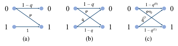
Figure 1: Three Channel Models: (a) the $Z$-channel models one-sided errors; (b) the binary symmetric channel models two-sided symmetric errors; (c) the general binary channel admits different probabilities $q^{(0)}$ for $0\to 1$ errors and $q^{(1)}$ for $1\to 0$ errors.

One-sided error: In the pairwise sequence alignment problem presented in Section 1, we want to recover the pairwise overlap fractions (or alignment scores) $p_{i}\in(0,1)$ between read $S_{0}$ and read $S_{i}$, for $i=1,...,n$. The observation for read pair $(S_{0},S_{i})$ and hash function $h_{j}$ is modelled by $Y_{i,j}\sim{\rm Ber}(p_{i})\vee{\rm Ber}(q_{j})$, which can be thought of as observing a ${\rm Ber}(p_{i})$ random variable through a Z-channel with crossover probability $q_{j}$. A Z-channel, shown in Fig. 1(a), is one where an input $1$ is never flipped but an input $0$ is flipped with some probability [13]. Hence, this models one-sided errors. If we process the data as $X:=Y-{\mathbf{1}}{\mathbf{1}}^{T}$, we then have that

$$\mathbb{E}[X]=({\mathbf{1}}-{\mathbf{p}})({\mathbf{q}}-{\mathbf{1}})^{T},$$ (7)

giving us ${\mathbf{u}}={\mathbf{1}}-{\mathbf{p}}$ and ${\mathbf{v}}={\mathbf{1}}-{\mathbf{q}}$. While, in this case, the entries $X_{i,j}$ are technically in $\{0,-1\}$, our main results (presented in Section 3 for a binary matrix $X\in\{0,1\}^{n\times m}$) can be readily extended.

Two-sided error: In the binary crowdsourcing problem, $n$ items have associated parameters $p_{i}\in(0,1)$ (the population rating of the item), for $i=1,...,n$. The observation of the rating of worker $j$ on the $i$th item is modelled as $Y_{i,j}\sim{\rm Ber}(p_{i})\oplus{\rm Ber}(q_{j}),$ where $\oplus$ represents the XOR operation. This can be thought of as observing a ${\rm Ber}(p_{i})$ random variable through a Binary Symmetric Channel with crossover probability $q_{j}$. A Binary Symmetric Channel, shown in Fig. 1(b), is one where the probability of flipping $1$ to $0$ and $0$ to $1$ is the same. The processed data in this case is $X:=Y-\frac{1}{2}{\mathbf{1}}{\mathbf{1}}^{T}$, and the expected value of our observation matrix is given by

$$\mathbb{E}[X]=\left({\mathbf{p}}-\tfrac{1}{2}{\mathbf{1}}\right)({\mathbf{1}}-2{\mathbf{q}})^{T},$$ (8)

giving us ${\mathbf{u}}={\mathbf{p}}-\frac{1}{2}{\mathbf{1}}$ and ${\mathbf{v}}={\mathbf{1}}-2{\mathbf{q}}$. As in the case of one-sided errors, the observations $X_{i,j}$ are not in $\{0,1\}$ but they only take two values and the results in Section 3 still hold.

Notice that if we do not make the assumption of symmetry and use a general binary channel, shown in Fig. 1(c), the model is still low-rank (it is rank-$2$) in expectation. In this manuscript, we focus on rank-one models, but briefly discuss this generalization in Appendix A.

Model Identifiability: Strictly speaking, the models described above are not identifiable, unless extra information is provided. This is because $\|{\mathbf{u}}\|$ and $\|{\mathbf{v}}\|$ are unspecified, and replacing ${\mathbf{u}}$ and ${\mathbf{v}}$ with $\alpha{\mathbf{u}}$ and $\frac{1}{\alpha}{\mathbf{v}}$ leads to the same distribution for the observation matrix $X$.

In practice one can overcome this issue by including questions with known answers. For the pairwise sequence alignment problem of Baharav et al. [5], the authors add “calibration reads” to the dataset. These are random reads, expected to have zero overlap with other reads in the dataset. In a crowdsourcing setting one similarly can add questions whose answers are known to the dataset. Based on questions with known answers, it is possible accurately estimate the “average expertise” of the workers, captured by $\|{\mathbf{v}}\|$. In order to avoid overcomplicating the model and the results and to circumvent the unidentifiability issue, we assume that $\|{\mathbf{v}}\|$ is known in our theoretical analysis. In our experiments, we adopt the known-questions strategy to estimate $\|{\mathbf{v}}\|$.

3 Spectral Estimators

Consider the general rank-one model described in Section 2. The $n\times m$ binary matrix of observations $X$ can be written as $X={\mathbb{E}}[X]+W,$ where ${\mathbb{E}}[X]={\mathbf{u}}{\mathbf{v}}^{T}$. We assume throughout this section that $u_{i},v_{j}\in[c,C]$, where $0<c<C<1$. Moreover, we assume that $\|{\mathbf{v}}\|$ is known, in order to make the model identifiable, as described in Section 2.

A natural estimator for ${\mathbf{u}}$ is the leading left singular vector of $X$ (or the leading eigenvector of $XX^{T}$), rescaled to have the same norm as ${\mathbf{u}}$. One issue with such an estimator is that it is not straightforward to obtain confidence intervals for each of its entries. There is a fair amount of work in constructing $\ell_{2}$ confidence intervals around eigenvectors of perturbed matrices [12, 10, 9]. However, the translation of $\ell_{2}$ control over eigenvectors to element-wise control using standard bounds costs us a $\sqrt{n}$ factor, which makes the resulting bounds too loose for the purposes of adaptive algorithms, which we will explore in Section 4. There has been some work on directly obtaining $\ell_{\infty}$ control for eigenvectors by Abbe et al. [1], Fan et al. [18]. However, they analyse a slightly different quantity, and so a direct application of these results to our rank-one models does not give us the desired element-wise control.

In order to overcome this issue and obtain element-wise confidence bounds on our estimate of each $u_{i}$, we propose a variation on the standard spectral estimator for ${\mathbf{u}}$. To provide intuition to our method, let us consider a simpler setting – one where we know ${\mathbf{v}}$ exactly. In this case a popular means to estimate ${\mathbf{u}}$ is the matched filter estimator [44]

$$\hat{u}_{i} =X_{i,.}\frac{{\mathbf{v}}}{\|{\mathbf{v}}\|^{2}},$$ (9)

where $X_{i,.}$ is the $i$th row of $X$. It is easy to see that $\hat{u}_{i}$ is an unbiased estimator of $u_{i}$, and standard concentration inequalities can be used to obtain confidence intervals. We try to mimic this intuition by splitting the rows of the matrix into two – red rows and blue rows. We then use the red rows to obtain an estimate $\hat{\mathbf{v}}$ of ${\mathbf{v}}$. We treat this as the true value of ${\mathbf{v}}$ and obtain the matched filter estimate for the $u_{i}$s corresponding to the blue rows, which gives us element-wise confidence intervals. We then use the blue rows to estimate ${\mathbf{v}}$, and apply the matched filter to obtain estimates for the $u_{i}$s corresponding to the red rows. This is summarised in the following algorithm.

1:Input: $X\in\{0,1\}^{n\times m}$, $\|{\mathbf{v}}\|$

2:Split $X$ into two $\tfrac{n}{2}\times m$ matrices $X_{A}$ and $X_{B}$

3:$\hat{\mathbf{v}}_{A}\leftarrow$ leading right singular vector of $X_{A}$

4:$\hat{\mathbf{v}}_{B}\leftarrow$ leading right singular vector of $X_{B}$

5:$\hat{\mathbf{u}}_{A}\leftarrow X_{A}\frac{\hat{\mathbf{v}}_{B}}{\|\hat{\mathbf{v}}_{B}\|\|{\mathbf{v}}\|}$,  $\hat{\mathbf{u}}_{B}\leftarrow X_{B}\frac{\hat{\mathbf{v}}_{A}}{\|\hat{\mathbf{v}}_{A}\|\|{\mathbf{v}}\|}$

6:return $\hat{\mathbf{u}}=\begin{bmatrix}\hat{{\mathbf{u}}}_{A}\\ \hat{{\mathbf{u}}}_{B}\end{bmatrix}$

Algorithm 1 Spectral estimation of ${\mathbf{u}}$

The main result in this section is an element-wise confidence interval for the resulting $\hat{{\mathbf{u}}}$.

Theorem 1.

When given $X$ and $\|{\mathbf{v}}\|$ as inputs, Algorithm 1 returns $\hat{{\mathbf{u}}}=[\hat{u}_{1},...,\hat{u}_{m}]^{T}$ satisfying

$${\mathbb{P}}\left(|\hat{u}_{i}-u_{i}|>\epsilon\right) \leq 3n\exp\left(-C_{1}{m\epsilon^{2}}\right),$$ (10)

for $i\in\{1,...,n\}$, $0<{\epsilon}<1$, $m\leq n$, and constant $C_{1}$ specified in Appendix G.

In the remainder of this section, we describe the key technical results required to prove Theorem 1. We discuss the application of these confidence intervals to create an adaptive algorithm in Section 4.

To prove Theorem 1 we first establish a connection between $\ell_{2}$ control of $\hat{{\mathbf{v}}}$ and element-wise control of $\hat{{\mathbf{u}}}$. Then we provide expectation and tail bounds for the $\ell_{2}$ error in $\hat{{\mathbf{v}}}$. For ease of exposition, we will drop the subscripts $A$ and $B$ in $X_{A}$, $X_{B}$, $\hat{{\mathbf{v}}}_{A}$, and $\hat{{\mathbf{v}}}_{B}$. We will implicitly assume that $X$ and $\hat{{\mathbf{v}}}$ correspond to distinct halves of the data matrix, thus being independent. The main technical ingredient required to establish Theorem 1 is the following lemma.

Lemma 1.

The error of estimator $\hat{{\mathbf{u}}}$ satisfies

$$\|\hat{{\mathbf{u}}}-{\mathbf{u}}\|_{\infty}\leq\frac{1}{\|{\mathbf{v}}\|}\left|\sum_{j=1}^{m}\left(X_{i,j}-u_{i}v_{j}\right){\mathbb{E}}\left[\frac{\hat{v}_{j}}{\|\hat{{\mathbf{v}}}\|}\right]\right|+\frac{1}{c}\left\|\frac{\hat{{\mathbf{v}}}}{\|\hat{{\mathbf{v}}}\|}-\frac{{\mathbf{v}}}{\|{{\mathbf{v}}}\|}\right\|+\frac{2}{c}\,{\mathbb{E}}\left\|\frac{\hat{{\mathbf{v}}}}{\|\hat{{\mathbf{v}}}\|}-\frac{{\mathbf{v}}}{\|{{\mathbf{v}}}\|}\right\|.$$

Notice that the right-hand side of the bound in Lemma 1 (proved in Appendix B) involves the $\ell_{2}$ error of $\hat{\mathbf{v}}$, and can in turn be used to bound the $\ell_{\infty}$ error of the estimator $\hat{\mathbf{u}}$. The first term in the bound is a sum of independent, bounded, zero-mean random variables $(X_{i,j}-u_{i}v_{j}){\mathbb{E}}[\hat{v}_{j}/\|\hat{{\mathbf{v}}}\|]$, for $j=1,...,m$. Using Hoeffding’s inequality, we show in Appendix C that, for any ${\epsilon}>0$,

$${\mathbb{P}}\left(\left|\textstyle{\sum_{j=1}^{m}}(X_{i,j}-u_{i}v_{j}){\mathbb{E}}[\hat{v}_{j}/\|\hat{{\mathbf{v}}}\|]\right|>\|{\mathbf{v}}\|{\epsilon}\right)\leq 2\exp\left(-{2c^{2}m{\epsilon}^{2}}\right).$$ (11)

In order to bound the second and third terms on the right-hand side of Lemma 1, we resort to matrix concentration inequalities and the Davis-Kahan theorem [15]. More precisely, we have the following lemma, which we prove in Appendix D.

Lemma 2.

The error of estimator $\hat{{\mathbf{v}}}$ satisfies

1. ${\mathbb{P}}\left(\left\|\frac{\hat{{\mathbf{v}}}}{\|\hat{{\mathbf{v}}}\|}-\frac{{\mathbf{v}}}{\|{\mathbf{v}}\|}\right\|\geq\epsilon\right)\leq(m+n)\exp\left(-C_{2}{\epsilon}^{2}\min(m,n)\right)$,  for $0<{\epsilon}<1$,

2. ${\mathbb{E}}\left\|\frac{\hat{{\mathbf{v}}}}{\|\hat{{\mathbf{v}}}\|}-\frac{{\mathbf{v}}}{\|{\mathbf{v}}\|}\right\|\leq C_{3}\sqrt{\frac{\log(m+n)}{\min(m,n)}}$,

where $C_{2}$ and $C_{3}$ are constants specified in Appendix G.

Given (11) and the bounds in Lemma 2, it is straightforward to establish Theorem 1, as we do next. Fixing some ${\epsilon}\in(0,1)$, we have that if ${\epsilon}^{2}\min(m,n)>(6C_{3}/c)^{2}\log(m+n)$, then Lemma 2(b) implies that

$$\frac{2}{c}\,{\mathbb{E}}\left\|\frac{\hat{{\mathbf{v}}}}{\|\hat{{\mathbf{v}}}\|}-\frac{{\mathbf{v}}}{\|{\mathbf{v}}\|}\right\|\leq\frac{2C_{3}}{c}\sqrt{\frac{\log(m+n)}{\min(m,n)}}<\frac{{\epsilon}}{3}.$$

Hence, if ${\epsilon}^{2}\min(m,n)>(6C_{3}/c)^{2}\log(m+n)$,

$${\mathbb{P}}\left(|\hat{u}_{i}-u_{i}|>\epsilon\right) \leq{\mathbb{P}}\left(\left|\sum_{j=1}^{m}(X_{i,j}-u_{i}v_{j}){\mathbb{E}}\left[\frac{\hat{v}_{j}}{\|\hat{{\mathbf{v}}}\|}\right]\right|>\frac{\|{\mathbf{v}}\|{\epsilon}}{3}\right)+{\mathbb{P}}\left(\left\|\frac{\hat{{\mathbf{v}}}}{\|\hat{{\mathbf{v}}}\|}-\frac{{\mathbf{v}}}{\|{\mathbf{v}}\|}\right\|\geq\frac{c{\epsilon}}{3}\right)$$

$$\leq 2\exp\left(-\frac{c^{2}m{\epsilon}^{2}}{18}\right)+(m+n)\exp\left(-C_{2}\frac{c^{2}\epsilon^{2}\min(m,n)}{9}\right)$$

$$\leq(m+n+2)\exp\left(-C_{4}\min(m,n){\epsilon^{2}}\right).$$ (12)

Notice that (12) is a vacuous statement whenever $C_{4}{\epsilon}^{2}\min(m,n)<\log(m+n)$, as the right-hand side is greater than $1$. Hence, if we replace $C_{4}$ with $C_{1}=\min[C_{4},(6C_{3}/c)^{-2}]$, the inequality holds for all $m$ and $n$. The result in Theorem 1 then follows by assuming $m\leq n$.

4 Leveraging confidence intervals for adaptivity

In the pairwise sequence alignment problem, one is typically only interested in identifying pairs of reads with large overlaps. Hence, by discarding pairs of reads with a small overlap based on a coarse alignment estimate and adaptively picking the pairs of reads for which a more accurate estimate is needed, it is possible to save significant computational resources. Similarly, in crowdsourcing applications, one may be interested in employing adaptive schemes in order to effectively use worker resources to identify only the most popular items.

We consider two natural problems that can be addressed within an adaptive framework. The first one is the identification of the top-$k$ largest alignment scores. In the second problem, the goal is to return a list of reads with high pairwise alignment to the reference, i.e., all reads with $u_{i}$ above a certain threshold. More generally, we consider the task of identifying a set of reads including all reads with pairwise alignment above $\alpha$ and no reads with pairwise alignment below $\beta$, for some $\beta\leq\alpha$. Adaptivity in the first problem can be achieved by casting the problem as a top-$k$ multi-armed bandit problem, while the second problem can be cast as a Thresholding Bandit problem [32].

4.1 Identifying the top-$k$ alignments:

We consider the setting where we wish to find the $k$ largest pairwise alignments with a given read. We assume that we have a total computational budget of $T$ min-hash comparisons. Notice that the regime where $T<n$ is uninteresting as we cannot even make one min-hash comparison per read. When $T=\Omega(n)$, a simple non-adaptive approach is to divide our budget $T$ evenly among all reads (as done in [5]). This gives us an $n\times\frac{T}{n}$ min-hash collision matrix $X$, from which we can estimate $\hat{\mathbf{u}}$ using Algorithm 1 and choose the top $k$ alignments based on their $\hat{u}_{i}$ values. Let $u_{(1)}\geq u_{(2)}\geq...\geq u_{(n)}$ be the sorted entries of the true ${\mathbf{u}}$ and define $\Delta_{i}=u_{(i)}-u_{(k)}$ for $i=1,...,n$. Notice that the non-adaptive approach recovers $u_{(1)},...,u_{(k)}$ correctly if each $\hat{u}_{i}$ stays within $\Delta_{k+1}$ of its true value $u_{i}$. From the union bound and Theorem 1,

$${\mathbb{P}}(\text{failure}) \leq\sum_{i=1}^{n}{\mathbb{P}}\left(|\hat{u}_{i}-u_{i}|>\Delta_{k+1}/2\right)\leq 3n^{2}\exp\left(-\frac{C_{1}}{4}\frac{\Delta_{k+1}^{2}T}{n}\right),$$ (13)

if $n\leq T\leq n^{2}$. Hence, the budget required to achieve an error probability of $\delta$ is

$$T=O\left({\Delta_{k+1}^{-2}}n\log\left(\tfrac{n}{\delta}\right)\right).$$ (14)

Moreover, from (13), we see that a budget $T=n\log^{\beta}n$, $\beta>1$, allows you to correctly identify the top-$k$ alignments if $(\Delta_{k+1}^{2}T)/n\approx\log n$, or $\Delta_{k+1}\approx{\log^{-(\beta-1)/2}}n$. Hence, the budget $T$ places a constraint in the minimum gap $\Delta_{k+1}$ that can be resolved.

Next we propose an adaptive way to allocate the same budget $T$. Algorithm 2 builds on an approach by Karnin et al. [28], but incorporates the spectral estimation approach from Section 3. The algorithm assumes the regime $n\log n<T<n^{2}$.

1:Input: $T$, $k$

2:$\text{Initialize }{\mathcal{I}}_{0}\leftarrow\{1,2,...,n\}$ $\triangleright$ Initial set of candidates

3:for $r=0$ to $r_{\rm max}\triangleq\lceil\log_{2}\frac{n}{\sqrt{T}.}\rceil-1$ do

4:     $\displaystyle t_{r}\leftarrow\left\lfloor\frac{T}{2|{\mathcal{I}}_{r}|\lceil\log_{2}\frac{n}{\sqrt{T}}\rceil}\right\rfloor$ $\triangleright$ Number of samples to be taken

5:     Obtain a binary matrix $X^{(r)}\in\{0,1\}^{|{\mathcal{I}}_{r}|\times t_{r}}$ and corresponding $\|{\mathbf{v}}^{(r)}\|$

6:     Use Algorithm 1 to compute estimates $\hat{{\mathbf{u}}}^{(r)}$ for $X^{(r)}$

7:     Set ${\mathcal{I}}_{r+1}$ to be the $\lceil|{\mathcal{I}}_{r}|/2\rceil$ coordinates in ${\mathcal{I}}_{r}$ with largest $\hat{{\mathbf{u}}}^{(r)}$

8:Clean up: Use $t_{r_{\max}+1}=\frac{T}{2}$, and compute $\hat{{\mathbf{u}}}^{(r_{\rm max}+1)}$ as above

9:return the $k$ coordinates of ${\mathcal{I}}_{r_{\rm max}+1}$ with the largest $\hat{{\mathbf{u}}}^{(r_{\rm max}+1)}$

Algorithm 2 Adaptive Spectral Top-$k$ Algorithm

At the $r$-th iteration, Algorithm 2 uses $t_{r}$ new hash functions and computes the min-hash collisions for the reads in ${\mathcal{I}}_{r}$, which are represented by the matrix $X^{(r)}$. Notice that we assume that the $t_{r}$ min-hashes in each iteration are different, which makes observation matrices $X^{(r)}$ all independent. Also, we assume that the $\ell_{2}$ norm of the right singular vector of ${\mathbb{E}}X^{(r)}$, $\|{\mathbf{v}}^{(r)}\|$, can be obtained exactly at each iteration of the algorithm. As discussed in Section 2, this makes the model identifiable and can be emulated in practice with calibration reads. At each iteration, Algorithm 2 eliminates half of the reads in ${\mathcal{I}}_{r}$. After $r_{\rm max}+1$ iterations, the number of remaining reads satisfies $\sqrt{T}/2\leq|{\mathcal{I}}_{r_{\rm max}+1}|\leq 2\sqrt{T}$, and the total budget used is $\sum_{r=0}^{r_{\rm max}}|{\mathcal{I}}_{r}|t_{r}\leq T/2$. Finally, in the “clean up” stage, we use the remaining $T/2$ budget to obtain the top $k$ among the approximately $\sqrt{T}$ remaining items. Notice that the final observation matrix is approximately $\sqrt{T}\times\sqrt{T}$.

In order to analyse the performance of Algorithm 2, we proceed simiarly to Karnin et al. [28], and define $H_{2}=\max_{i>k}\frac{i}{\Delta_{i}^{2}}.$ We then have the following performance guarantee (proof in Appendix E).

Theorem 2.

Given budget $n\log n\leq T\leq n^{2}$ and assuming $2k<\sqrt{T}$, Algorithm 2 correctly identifies the top $k$ alignments with probability at least

$$1-18kn\log n\exp\left(-\frac{C_{1}}{64}\frac{T}{H_{2}\log n}\right)-12n^{2}\exp\left(-\frac{C_{1}}{16}\Delta_{k+1}^{2}\sqrt{T}\right)$$ (15)

Moreover, for sufficiently small $\delta$, Algorithm 2 achieves an error probability of at most $\delta$ with budget

$$T=O\left(H_{2}\log n\log\left(nk\frac{\log n}{\delta}\right)+\Delta_{k+1}^{-4}\log^{2}\left(\frac{n^{2}}{\delta}\right)\right).$$ (16)

Comparing (15) and (16) with the non-adaptive counterparts (13) and (14) requires a handle on $H_{2}$. This quantity captures how difficult it is to separate the top $k$ alignments, and satisfies $(k+1)\Delta_{k+1}^{-2}\leq H_{2}\leq n\Delta_{k+1}^{-2}$. The extreme case $H_{2}\approx n\Delta_{k+1}^{-2}$ occurs when all of the $n-k$ suboptimal items have very similar qualities. In this case, adaptivity is not helpful. However, when $u_{(k+1)}$ is large compared to other non-top-$k$ alignments, we are in the $H_{2}\approx k\Delta_{k+1}^{-2}$ regime. Then the budget requirements are essentially $T=O(k\Delta_{k+1}^{-2}\log^{2}n+\Delta_{k+1}^{-4}\log^{2}n)$, which is $O(\Delta_{k+1}^{-4}\log^{2}n)$ for $k,\delta$ constant. Furthermore, in the $H_{2}\approx k\Delta_{k+1}^{-2}$ regime, a budget $T=n\log^{\beta}n$, $\beta>2$, allows you to correctly identify the top-$k$ alignments with a gap of $\Delta_{k+1}\approx n^{-1/4}$ which is significantly smaller than the $\Delta_{k+1}\approx{\log^{-(\beta-1)/2}}n$ afforded in the non-adaptive case. As a concrete example, suppose that out of the $n$ alignments, there are $k$ highly overlapping reads with $u_{i}=C$, $k$ moderately overlapping reads with $u_{i}=C-n^{-1/4}$, and $n-2k$ reads with no overlap and $u_{i}=c$. In this case, Algorithm 2 requires a budget of $T=O\left(n\log^{2}\left(\frac{n}{\delta}\right)\right)$, while the non-adaptive approach requires $T=O\left((n^{3/2}\log\left(\frac{n}{\delta}\right)\right)$.

4.2 Identifying all alignments above a threshold:

In this section, we develop a bandit algorithm to return a set of coordinates in $\{1,...,n\}$ such that with high probability all coordinates with $u_{i}\geq\beta$ are returned and no coordinates with $u_{i}\leq\alpha$ are returned, for some $\beta>\alpha$. We assume that $\beta-\alpha>\sqrt{\frac{12\log n}{C_{4}n}}$. The algorithm and analysis follow similarly to Locatelli et al. [32].

Lemma 3.

For any $\Gamma\in{\mathbb{R}}$, our estimates $\hat{u}_{i}$ from Algorithm 1 run with an $n\times m$ matrix with $m,n$ such that

$$\min(m,n) \geq\frac{\log\left(\frac{1}{\delta}\right)+\log(m+n+2)}{\Gamma^{2}C_{4}},$$ (17)

will have $|\hat{u}_{i}-u_{i}|\leq\Gamma$ with probability at least $1-\delta$. Thus, if

$$\min(m,n) \geq\frac{3\log n+2\log(m+n)}{\Gamma^{2}C_{4}}$$ (18)

then with probability $1-\frac{1}{n^{2}}$, $|\hat{u}_{i}-u_{i}|\leq\Gamma$ for all $i\in\{1,...,n\}$.

Proof.

Eq. (17) follows by inverting the error bound from Eq. (12). Eq. (18) follows by just substituting $\delta=\frac{1}{n^{3}}$ and noting that $\log(m+n+2)\leq 2\log(m+n)$ as long as $m+n\geq 4$. ∎

Notice that a naive non-adaptive approach to this thresholding problem would consist of applying Algorithm 1 to the entire observation matrix, with enough enough workers such that the confidence intervals are smaller than $\frac{\beta-\alpha}{2}$ and return coordinates with value more than $\frac{\alpha+\beta}{2}$. In that case, Lemma 3 implies that $\frac{12}{C_{4}}\frac{n\log n}{(\beta-\alpha)^{2}}$ workers’ responses are enough to succeed with probability at least $1-\frac{1}{n}$. In Algorithm 3, we propose an adaptive way of performing the same task.

1:Input: Range $[\alpha,\beta]$.

2:$\text{Initialise }S_{0}\leftarrow\{1,...,n\}$ $\triangleright$ Set of coordinates initially under consideration

3:$\text{Initialise }A\leftarrow\emptyset$ $\triangleright$ Set of coordinates initially accepted

4:$t_{-1}\leftarrow\frac{12\log n}{C_{4}}$ $\triangleright$ Initial number of workers recruited. $C_{4}$ from Eq. (17)

5:for $r=0$ to $\lceil\log_{2}\frac{1}{\beta-\alpha}\rceil-1$ do

6:     $t_{r}=4t_{r-1}$ $\triangleright$ Number of workers to be recruited

7:     Obtain a binary response matrix $X^{(r)}\in\{0,1\}^{|S_{r}|\times t_{r}}$ and corresponding $\|{\mathbf{v}}^{(r)}\|$

8:     Use Algorithm 1 to compute estimates $\hat{{\mathbf{u}}}^{(r)}$ for $X^{(r)}$

9:     Construct confidence intervals $C(t_{r})$ (same for every question)

10:     Construct accepted set $C_{\rm acc}=\{i\in S_{r}:\hat{u}^{(r)}_{i}-C(t_{r})>\alpha\}$

11:     Construct rejected set $C_{\rm rej}=\{i\in S_{r}:\hat{u}^{(r)}_{i}+C(t_{r})<\beta\}$

12:     Set $S_{r+1}=S_{r}\setminus\left\{C_{\rm rej}\cup C_{\rm acc}\right\}$

13:     if $|S_{r+1}|<\frac{12}{(\beta-\alpha)^{2}C_{4}}\log n$ then

14:         Let ${\mathcal{I}}$ be $\frac{12}{(\beta-\alpha)^{2}C_{4}}\log n-|S_{r+1}|$ coordinates of $C_{\rm rej}\cup C_{\rm acc}$ picked uniformly at random.

15:         $S_{C}=S_{r+1}\cup{\mathcal{I}}$

16:         $A=A\cup(C_{\rm acc})$

17:         break

18:     else

19:         Set $A=A\cup C_{\rm acc}$      

20:Clean up: Use $t_{C}=\frac{12\log n}{(\beta-\alpha)^{2}C_{4}}$ workers with set $S_{C}$ of questions to obtain estimates $\hat{{\mathbf{u}}}^{(C)}$. Construct confidence intervals $C(t_{C})$ and accepted set $C_{A}=\{i\in S_{C}:\hat{u}^{(C)}_{i}-C(t_{C})>\alpha\}$

21:return $A\cup C_{A}$.

Algorithm 3 Adaptive Spectral Thresholding Algorithm

Remark 1.

Line 14 is used to make sure that we have $n>m$ in the clean up stage. Selecting ${\mathcal{I}}$ uniformly at random from $C_{\rm rej}\cup C_{\rm acc}$ is simply given as a concrete way for the algorithm to run.

Let $\kappa:=\left\lfloor\frac{12}{(\beta-\alpha)^{2}C_{4}}\log n\right\rfloor$. Define

$$\Gamma_{i} =\begin{cases}u_{i}-\alpha&\text{ if }\beta<u_{i},\\ \beta-\alpha&\text{ if }\alpha\leq u_{i}\leq\beta,\\ \beta-u_{i}&\text{ if }u_{i}<\alpha.\end{cases}$$ (19)

See Figure 2 for an illustration. Further let $\Gamma^{(1)}\leq\Gamma^{(2)}\leq\cdots\leq\Gamma^{(n)}$ be the sorted list of the $\Gamma_{i}$.

Figure 2: An illustration of $\Gamma_{i}$ of Eq. (19)

Theorem 3.

Given parameters $\beta$ and $\alpha$ such that $\beta-\alpha>\sqrt{\frac{12\log n}{C_{4}n}}$, with probability at least $1-\frac{2}{n}$ Algorithm 3 will output a set of reads $R$ such that $\{i:u_{i}>\beta\}\subseteq R\subseteq\{i:u_{i}>\alpha\}$ and use budget

$$T\leq 2\left(\frac{12}{C_{4}}\frac{\log n}{(\beta-\alpha)^{2}}\right)^{2}+\sum_{\ell=\kappa+1}^{n}\frac{32}{C_{4}}\frac{\log n}{(\Gamma^{(\ell)})^{2}}$$ (20)

where $\Gamma_{i}$ denotes the difficulty of classifying $u_{i}$, with $\Gamma^{(1)}\leq\cdots\leq\Gamma^{(n)}$ as the sorted list of the $\Gamma_{i}$.

The proof of the theorem is in Appendix F.

Remark 2.

Theorem 3 enables us to construct confidence intervals of $\frac{\beta-\alpha}{2}$ for only the “most borderline” $\kappa$ questions and near optimal confidence intervals for the rest, while the non-adaptive algorithm would need to construct confidence intervals of $\frac{\beta-\alpha}{2}$ for all.

5 Empirical Results

In order to validate the Adaptive Spectral Top-$k$ algorithm, we conducted two types of experiments:

1. controlled experiments on simulated data for a crowdsourcing model with symmetric errors;

2. pairwise sequence alignment experiments on real DNA sequencing data.

We consider the top-$k$ identification problem with $k=5$ in both cases. We run Algorithm 2 with some slight modifications, namely halving until we have fewer than $2k$ remaining arms before moving to the clean up step, and compare its performance with the non-adaptive spectral approach. Further experimental details are in Appendix I. We measure success in two ways. First, we consider the error probability of returning the top $k$ items (i.e., any deviation from the top-$k$ is considered a failure). Second, we consider a less stringent metric, where we allow the algorithm to return its top-$2k$ items, and we consider the fraction of the true top-$k$ items that are present to evaluate performance. Our code is publicly available online at github.com/TavorB/adaptiveSpectral.

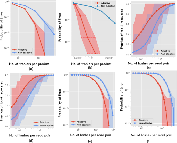
Figure 3: (a) shows the probability of error of the controlled crowdsourcing experiment as the number of workers per product is increased, where an error is defined as incorrectly identifying the set of top-$k$ products. (b) shows the same in the thresholding bandits setup. (c) shows the fraction of the top-$k$ reads that are in the $2k$ reads returned for the E. coli dataset, while (d) shows the fraction of the top-$k$ reads that are in the top-$k$ reads returned for the NCTC4174 dataset. (e) shows the probability of error of correctly identifying the set of top-$k$ overlaps on the E. coli dataset, while (f) shows the same for the NCTC4174 dataset. 1000 trials are conducted for each point. $95\%$ percentiles are shaded around each point in (b), (c) and (d) (note that confidence intervals for (b) are on the x-axis). For (a), (e) and (f), $\frac{1}{\sqrt{\text{number of trials}}}$ is shaded around each point. For further details, see Appendix I.

Controlled experiments: We consider a crowdsourcing scenario with symmetric errors as modelled in (8). We want to determine the $5$ best products from a list of $1000$ products. We generate the true product qualities (that is, the $p_{i}$ parameters) from a Beta$(1,5)$ distribution independent of each other. Each of the worker abilities $q_{j}$ is drawn from a Uniform$(0,1)$ distribution, independent of everything else. We consider the problem of top-$5$ product detection at various budgets as shown in Figure 3(a) with success rate measured by the presence in the top-$10$ items. We see that the adaptive algorithm requires significantly fewer worker responses to achieve equal performance to the non-adaptive one.

In Figure 3(b) we consider the same set up as above but in the fixed confidence setting, considering the problem of being able to detect all products that are liked by more than $65\%$ of the population while returning none that is liked by less than $50\%$ of the population. Again, we see that for the same probability of error the adaptive algorithm needs far fewer workers.

Real data experiments: Using the PacBio E. coli data set [38] that was examined in Baharav et al. [5] we consider the problem of finding, for a fixed reference read, the $5$ reads that have the largest alignment with the reference read in the dataset. We show the fraction of the $5$ reads that are present when returning $10$ reads in Figure 3(c) and the success probability when returning exactly $5$ reads in Figure 3(e) (i.e., the probability of returning exactly the top-$5$ reads). To achieve an error rate of 0.9% the non-adaptive algorithm requires over 8500 min-hash comparisons per read, while the adaptive algorithm requires fewer than 6000 per read to reach an error rate of 0.1%.

We also consider the NCTC4174 dataset of [39] and plot the fraction correct when returning $5$ reads in Figure 3(d) and the success probability when returning exactly $5$ reads in Figure 3(f). The results are qualitatively similar to what we observe in the case of the E. coli dataset.

6 Discussion

Motivated by applications in sequence alignment, we considered the problem of efficiently finding the largest elements in the left singular vector of a binary matrix $X$ with $\mathbb{E}[X]=\mathbf{u}\mathbf{v}^{T}$. To utilize the natural spectral estimator of $\mathbf{u}$, we designed a method to construct $\ell_{\infty}$ confidence intervals around the spectral estimator. To perform this spectral estimation efficiently, we leveraged multi-armed bandit algorithms to adaptively estimate the entries $u_{i}$ of the leading left singular vector to the necessary degree of accuracy. We show that this method provides computational gains on both real data and in controlled experiments.

Broader Impact

Over the last decade, high-throughput sequencing technologies have driven down the time and cost of acquiring biological data tremendously. This has caused an explosion in the amount of available genomic data, allowing scientists to obtain quantitative insights into the biology of all living organisms. Countless tasks – such as gene expression quantification, metagenomic sequencing, and single-cell RNA sequencing – heavily rely on some form of pairwise sequence alignment, which is a heavy computational burden and often the bottleneck of the analysis pipeline. The development of efficient algorithms for this task, which is the main outcome of this paper, is thus critical for the scalability of genomic data analysis.

From a theoretical perspective, this work establishes novel connections between a classical problem in bioinformatics (pairwise sequence alignment), spectral methods for parameter estimation from crowdsourced noisy data, and multi-armed bandits. This will help facilitate the transfer of insights and algorithms between these traditionally disparate areas. It will also add a new set of techniques to the toolbox of the computational biology community that we believe will find a host of applications in the context of genomics and other large-scale omics data analysis. Further, this work will allow other Machine Learning researchers unfamiliar with bioinformatics to utilise their expertise in solving new problems at this novel intersection of bioinformatics, spectral methods, and multi-armed bandits.

Appendix A A Rank-$2$ Model

Consider the case where we the $(i,j)$-th observation $Y_{i,j}$ is the output of a Ber$(p_{i})$ random variable passed through a general binary channel BC$(q^{(0)}_{j},q^{(1)}_{j})$ (see Figure 1(c)). Here $q^{(0)}_{j}$ is probability of a $0$ being flipped to a $1$ and $q^{(1)}_{j}$ is probability of a $1$ being flipped to a $0$ on the $j$th column.

We note that we have $n+2m$ parameters here, while a rank-one model would admit only $n+m$ parameters. Hence this is not a rank-one model. However we note that

$${\mathbb{E}}[Y] ={\mathbf{p}}({\mathbf{1}}-{\mathbf{q}}^{(0)})^{T}+({\mathbf{1}}-{\mathbf{p}}){\mathbf{q}}^{(1)T},$$ (21)

where ${\mathbf{p}}=[p_{1},...,p_{n}]^{T}$, ${\mathbf{q}}^{(0)}=[q^{(0)}_{1},...,q^{(0)}_{m}]^{T}$ and ${\mathbf{q}}^{(1)}=[q^{(1)}_{1},...,q^{(1)}_{m}]^{T}$. This shows that, when the noise in the workers’ responses is modelled by a general binary channel (see Figure 1(c)), we have a rank-$2$ model.

Appendix B Proof of Lemma 1

We start by using the triangle inequality to obtain

$$|\hat{u}_{i}-u_{i}|\leq|\hat{u}_{i}-{\mathbb{E}}[\hat{u}_{i}]|+|{\mathbb{E}}[\hat{u}_{i}]-u_{i}|.$$ (22)

To bound the first term, we first notice that since

$$\hat{u}_{i}=X_{i,.}\frac{\hat{{\mathbf{v}}}}{\|\hat{{\mathbf{v}}}\|\|{\mathbf{v}}\|}=\frac{1}{\|{\mathbf{v}}\|}\sum_{j=1}^{m}\left(X_{i,j}\frac{\hat{v}_{j}}{\|\hat{{\mathbf{v}}}\|}\right)$$ (23)

and $\hat{{\mathbf{v}}}$ is independent of $X_{i,.}$, we have that

$$\hat{u}_{i}-{\mathbb{E}}[\hat{u}_{i}] =\frac{1}{\|{\mathbf{v}}\|}\sum_{j=1}^{m}\left(X_{i,j}\frac{\hat{v}_{j}}{\|\hat{{\mathbf{v}}}\|}\right)-\frac{1}{\|{\mathbf{v}}\|}\sum_{j=1}^{m}\left(u_{i}v_{j}{\mathbb{E}}\left[\frac{\hat{v}_{j}}{\|\hat{{\mathbf{v}}}\|}\right]\right)$$

$$=\frac{1}{\|{\mathbf{v}}\|}\sum_{j=1}^{m}\left(X_{i,j}{\mathbb{E}}\left[\frac{\hat{v}_{j}}{\|\hat{{\mathbf{v}}}\|}\right]+X_{i,j}\left(\frac{\hat{v}_{j}}{\|\hat{{\mathbf{v}}}\|}-{\mathbb{E}}\left[\frac{\hat{v}_{j}}{\|\hat{{\mathbf{v}}}\|}\right]\right)-u_{i}v_{j}{\mathbb{E}}\left[\frac{\hat{v}_{j}}{\|\hat{{\mathbf{v}}}\|}\right]\right)$$

$$=\frac{1}{\|{\mathbf{v}}\|}\sum_{j=1}^{m}\left(X_{i,j}-u_{i}v_{j}\right){\mathbb{E}}\left[\frac{\hat{v}_{j}}{\|\hat{{\mathbf{v}}}\|}\right]+\frac{1}{\|{\mathbf{v}}\|}\sum_{j=1}^{m}X_{i,j}\left(\frac{\hat{v}_{j}}{\|\hat{{\mathbf{v}}}\|}-{\mathbb{E}}\left[\frac{\hat{v}_{j}}{\|\hat{{\mathbf{v}}}\|}\right]\right).$$ (24)

From the triangle inequality, we then have

$$|\hat{u}_{i}-{\mathbb{E}}[\hat{u}_{i}]| \leq\frac{1}{\|{\mathbf{v}}\|}\left|\sum_{j=1}^{m}\left(X_{i,j}-u_{i}v_{j}\right){\mathbb{E}}\left[\frac{\hat{v}_{j}}{\|\hat{{\mathbf{v}}}\|}\right]\right|+\frac{1}{\|{\mathbf{v}}\|}\sum_{j=1}^{m}|X_{i,j}|\left|\frac{\hat{v}_{j}}{\|\hat{{\mathbf{v}}}\|}-{\mathbb{E}}\left[\frac{\hat{v}_{j}}{\|\hat{{\mathbf{v}}}\|}\right]\right|$$

$$\leq\frac{1}{\|{\mathbf{v}}\|}\left|\sum_{j=1}^{m}\left(X_{i,j}-u_{i}v_{j}\right){\mathbb{E}}\left[\frac{\hat{v}_{j}}{\|\hat{{\mathbf{v}}}\|}\right]\right|+\frac{1}{\|{\mathbf{v}}\|}\left\|\frac{\hat{{\mathbf{v}}}}{\|\hat{{\mathbf{v}}}\|}-{\mathbb{E}}\left[\frac{\hat{{\mathbf{v}}}}{\|\hat{{\mathbf{v}}}\|}\right]\right\|_{1}$$ (25)

From the fact that $\|{\mathbf{v}}\|\geq c\sqrt{m}$ and the fact that $\|{\mathbf{x}}\|_{1}\leq\sqrt{m}\|{\mathbf{x}}\|_{2}$ for any ${\mathbf{x}}\in{\mathbb{R}}^{m}$, the second term can be bounded as

$$\frac{1}{\|{\mathbf{v}}\|}\left\|\frac{\hat{{\mathbf{v}}}}{\|\hat{{\mathbf{v}}}\|}-{\mathbb{E}}\left[\frac{\hat{{\mathbf{v}}}}{\|\hat{{\mathbf{v}}}\|}\right]\right\|_{1} \leq\frac{1}{c}\left\|\frac{\hat{{\mathbf{v}}}}{\|\hat{{\mathbf{v}}}\|}-{\mathbb{E}}\left[\frac{\hat{{\mathbf{v}}}}{\|\hat{{\mathbf{v}}}\|}\right]\right\|$$

$$\leq\frac{1}{c}\left\|\frac{\hat{{\mathbf{v}}}}{\|\hat{{\mathbf{v}}}\|}-\frac{{\mathbf{v}}}{\|{\mathbf{v}}\|}\right\|+\frac{1}{c}\left\|\frac{{\mathbf{v}}}{\|{\mathbf{v}}\|}-{\mathbb{E}}\left[\frac{\hat{{\mathbf{v}}}}{\|\hat{{\mathbf{v}}}\|}\right]\right\|$$

$$=\frac{1}{c}\left\|\frac{\hat{{\mathbf{v}}}}{\|\hat{{\mathbf{v}}}\|}-\frac{{\mathbf{v}}}{\|{\mathbf{v}}\|}\right\|+\frac{1}{c}\left\|{\mathbb{E}}\left[\frac{{\mathbf{v}}}{\|{\mathbf{v}}\|}-\frac{\hat{{\mathbf{v}}}}{\|\hat{{\mathbf{v}}}\|}\right]\right\|$$

$$\leq\frac{1}{c}\left\|\frac{\hat{{\mathbf{v}}}}{\|\hat{{\mathbf{v}}}\|}-\frac{{\mathbf{v}}}{\|{\mathbf{v}}\|}\right\|+\frac{1}{c}{\mathbb{E}}\left\|\frac{{\mathbf{v}}}{\|{\mathbf{v}}\|}-\frac{\hat{{\mathbf{v}}}}{\|\hat{{\mathbf{v}}}\|}\right\|,$$ (26)

where the last step follows from Jensen’s inequality.

Now we consider the second term in (22). We first notice that

$$\hat{u}_{i}=X_{i,.}\frac{\hat{{\mathbf{v}}}}{\|\hat{{\mathbf{v}}}\|\|{\mathbf{v}}\|}=\frac{X_{i,.}}{\|{\mathbf{v}}\|}\left(\frac{{\mathbf{v}}}{\|{\mathbf{v}}\|}+\frac{\hat{{\mathbf{v}}}}{\|\hat{{\mathbf{v}}}\|}-\frac{{\mathbf{v}}}{\|{\mathbf{v}}\|}\right)=\frac{X_{i,.}{\mathbf{v}}}{\|{\mathbf{v}}\|^{2}}+\frac{X_{i,.}}{\|{\mathbf{v}}\|}\left(\frac{\hat{{\mathbf{v}}}}{\|\hat{{\mathbf{v}}}\|}-\frac{{\mathbf{v}}}{\|{\mathbf{v}}\|}\right),$$

where we recognize the first term as the matched filter for estimating $u_{i}$ if ${\mathbf{v}}$ were known. Since $E[X_{i,.}]=u_{i}{\mathbf{v}}^{T}$ and $\hat{{\mathbf{v}}}$ is independent of $X_{i,.}$ (due to the splitting of the data matrix $X$), we have

$${\mathbb{E}}[\hat{u}_{i}]=\frac{u_{i}{\mathbf{v}}^{T}{\mathbf{v}}}{\|{\mathbf{v}}\|^{2}}+\frac{u_{i}{\mathbf{v}}^{T}}{\|{\mathbf{v}}\|}{\mathbb{E}}\left[\frac{\hat{{\mathbf{v}}}}{\|\hat{{\mathbf{v}}}\|}-\frac{{\mathbf{v}}}{\|{\mathbf{v}}\|}\right]=u_{i}+\frac{u_{i}{\mathbf{v}}^{T}}{\|{\mathbf{v}}\|}\left({\mathbb{E}}\left[\frac{\hat{{\mathbf{v}}}}{\|\hat{{\mathbf{v}}}\|}\right]-\frac{{\mathbf{v}}}{\|{\mathbf{v}}\|}\right).$$

Using the Cauchy-Schwarz inequality, we have that

$$\left|{\mathbb{E}}[\hat{u}_{i}]-u_{i}\right|\leq\frac{u_{i}\|{\mathbf{v}}\|}{\|{\mathbf{v}}\|}\left\|{\mathbb{E}}\left[\frac{\hat{{\mathbf{v}}}}{\|\hat{{\mathbf{v}}}\|}\right]-\frac{{\mathbf{v}}}{\|{\mathbf{v}}\|}\right\|=u_{i}\left\|{\mathbb{E}}\left[\frac{\hat{{\mathbf{v}}}}{\|\hat{{\mathbf{v}}}\|}\right]-\frac{{\mathbf{v}}}{\|{\mathbf{v}}\|}\right\|\leq u_{i}{\mathbb{E}}\left\|\frac{\hat{{\mathbf{v}}}}{\|\hat{{\mathbf{v}}}\|}-\frac{{\mathbf{v}}}{\|{\mathbf{v}}\|}\right\|,$$ (27)

where the last step follows from Jensen’s inequality.

Finally, putting together (22), (25), (26), and (27), and noting that $u_{i}<1<1/c$, we obtain

$$|\hat{u}_{i}-u_{i}|\leq\frac{1}{\|{\mathbf{v}}\|}\left|\sum_{j=1}^{m}\left(X_{i,j}-u_{i}\right)E\left[\frac{\hat{v}_{j}}{\|\hat{{\mathbf{v}}}\|}\right]\right|+\frac{1}{c}\left\|\frac{\hat{{\mathbf{v}}}}{\|\hat{{\mathbf{v}}}\|}-\frac{{\mathbf{v}}}{\|{{\mathbf{v}}}\|}\right\|+\frac{2}{c}\,{\mathbb{E}}\left\|\frac{\hat{{\mathbf{v}}}}{\|\hat{{\mathbf{v}}}\|}-\frac{{\mathbf{v}}}{\|{{\mathbf{v}}}\|}\right\|.$$

Appendix C Proof of Equation (11)

We claim that for any ${\epsilon}>0$,

$${\mathbb{P}}\left(\left|\textstyle{\sum_{j=1}^{m}}(X_{i,j}-u_{i}v_{j}){\mathbb{E}}[\hat{v}_{j}/\|\hat{{\mathbf{v}}}\|]\right|>\|{\mathbf{v}}\|{\epsilon}\right)\leq 2\exp\left(-{2c^{2}m{\epsilon}^{2}}\right).$$ (28)

First we notice that the random variables $(X_{i,j}-u_{i}v_{j}){\mathbb{E}}\left[\frac{\hat{v}_{j}}{\|\hat{{\mathbf{v}}}\|}\right]$, for $j=1,...,m$, are independent and zero-mean. Moreover, they satisfy

$$-u_{i}v_{j}{\mathbb{E}}\left[\frac{\hat{v}_{j}}{\|\hat{{\mathbf{v}}}\|}\right]<(X_{i,j}-u_{i}v_{j}){\mathbb{E}}\left[\frac{\hat{v}_{j}}{\|\hat{{\mathbf{v}}}\|}\right]<(1-u_{i}v_{j}){\mathbb{E}}\left[\frac{\hat{v}_{j}}{\|\hat{{\mathbf{v}}}\|}\right].$$

Using Hoeffding’s inequality, for any ${\epsilon}>0$ we have that

$${\mathbb{P}}\left(\left|\sum_{j=1}^{m}(X_{i,j}-u_{i}v_{j}){\mathbb{E}}\left[\frac{\hat{v}_{j}}{\|\hat{{\mathbf{v}}}\|}\right]\right|>\|{\mathbf{v}}\|{\epsilon}\right) \leq 2\exp\left(-\frac{2\|{\mathbf{v}}\|^{2}{\epsilon}^{2}}{\sum_{j=1}^{m}{\mathbb{E}}[\hat{v}_{j}/\|\hat{{\mathbf{v}}}\|]^{2}}\right)$$

$$\leq 2\exp\left(-\frac{2c^{2}m{\epsilon}^{2}}{{\mathbb{E}}\left[\sum_{j=1}^{m}\hat{v}_{j}^{2}/\|\hat{{\mathbf{v}}}\|^{2}\right]}\right)$$

$$=2\exp\left(-{2c^{2}m{\epsilon}^{2}}\right),$$

where in the second step we used Jensen’s inequality.

Appendix D Proof of Lemma 2

Let $W=X-{\mathbb{E}}X$ be the “noise” added to ${\mathbb{E}}X$. In order to prove Lemma 2, our first order of business is to bound the expectation of $\|W\|_{op}$ and $\|W\|_{op}^{2}$. Then we use these bounds with the Davis-Kahan theorem of Davis and Kahan [15] to bound the $\ell_{2}$ error in $\hat{{\mathbf{v}}}$. We have the following lemma.

Lemma 4.

The noise matrix $W=X-{\mathbb{E}}X$ satisfies

$${\mathbb{E}}\left[\|W\|_{op}\right]\leq 2\sqrt{(m+n)\log(m+n)}$$ (29)

$${\mathbb{E}}\left[\|W\|^{2}_{op}\right]\leq 120(m+n)\log(m+n)$$ (30)

Proof.

Strictly speaking, due to Jensen’s inequality, (30) implies (29) (with a different constant). However, to provide intuition and improve the exposition, we provide a standalone proof of (29) first. We start by noticing that

$$W_{i,j} =\begin{cases}1-u_{i}v_{j}&\text{ with probability }u_{i}v_{j},\\ -u_{i}v_{j}&\text{ with probability }1-u_{i}v_{j},\end{cases}$$

Hence we have

$$(\mathbb{E}[W^{T}W])_{i,j} =\begin{cases}0&\text{ if }i\neq j,\\ \sum_{k=1}^{n}u_{k}v_{i}(1-u_{k}v_{i})&\text{ if }i=j,\end{cases}$$

which implies that $c^{2}(1-C^{2})n\leq(\mathbb{E}[W^{T}W])_{i,i}\leq C^{2}(1-c^{2})n$. Thus $\|\mathbb{E}[W^{T}W]\|_{op}\in[c^{2}(1-C^{2})n,C^{2}(1-c^{2})n]$. Similarly one can argue that $\|\mathbb{E}[WW^{T}]\|_{op}\in[c^{2}(1-C^{2})m,C^{2}(1-c^{2})m]$. Following the notation of Tropp [43, Theorem 6.1.1], the matrix variance statistic $\nu(W)$ is

$$\nu(W) =\max\left(\|\mathbb{E}[W^{T}W]\|_{op},\|\mathbb{E}[WW^{T}]\|_{op}\right),$$

$$\in[c^{2}(1-C^{2})\max(m,n),C^{2}(1-c^{2})\max(m,n)],$$

$$\leq C^{2}(1-c^{2})(m+n)\leq m+n.$$ (31)

From the Matrix-Bernstein inequality [43, Eq. (6.1.3)], we have that

$${\mathbb{E}}\|W\|_{op} \leq\sqrt{2\nu(W)\log(m+n)}+\tfrac{1}{3}\log(m+n)$$

$$=\sqrt{2(m+n)\log(m+n)}+\tfrac{1}{3}\log(m+n)$$

$$\leq(\sqrt{2}+\tfrac{1}{3})\sqrt{(m+n)\log(m+n)}\leq 2\sqrt{(m+n)\log(m+n)},$$

proving (29). To prove (30), we rely on another inequality by Tropp [43, Eq. (6.1.6)] to state that

$$\left({\mathbb{E}}\|W\|_{op}^{2}\right)^{1/2} \leq\sqrt{2e\nu(W)\log(m+n)}+4e\log(m+n)$$

$$\leq\sqrt{2e(m+n)\log(m+n)}+4e\log(m+n)$$

$$\leq 4e\sqrt{(m+n)\log(m+n)},$$

which implies that ${\mathbb{E}}\|W\|_{op}^{2}\leq 120(m+n)\log(m+n)$, proving (30). ∎

With Lemma 4, we proceed to the proof of Lemma 2. Notice that the leading right singular vector of $X$ is equivalent to the leading eigenvector of $X^{T}X$. Also note that

$$X^{T}X =(\mathbb{E}X+W)^{T}(\mathbb{E}X+W)$$

$$=({\mathbf{u}}{\mathbf{v}}^{T}+W)^{T}({\mathbf{u}}{\mathbf{v}}^{T}+W)$$

$$=\|{\mathbf{u}}\|^{2}{\mathbf{v}}{\mathbf{v}}^{T}+{\mathbf{v}}{\mathbf{u}}^{T}W+W^{T}{\mathbf{u}}{\mathbf{v}}^{T}+W^{T}W.$$ (32)

We will use the Davis-Kahan theorem to bound $\left\|\frac{\hat{{\mathbf{v}}}}{\|\hat{{\mathbf{v}}}\|}-\frac{{\mathbf{v}}}{\|{\mathbf{v}}\|}\right\|$. We begin by bounding the operator norm of the “error terms” in (32) as

$$\|{\mathbf{v}}{\mathbf{u}}^{T}W+W^{T}{\mathbf{u}}{\mathbf{v}}^{T}+W^{T}W\|_{op} \overset{(a)}{\leq}\|{\mathbf{v}}{\mathbf{u}}^{T}W\|_{op}+\|W{\mathbf{u}}{\mathbf{v}}^{T}\|_{op}+\|W^{T}W\|_{op},$$

$$\overset{(b)}{\leq}\|{\mathbf{v}}{\mathbf{u}}^{T}\|_{op}\|W\|_{op}+\|W\|_{op}\|{\mathbf{u}}{\mathbf{v}}^{T}\|_{op}+\|W^{T}W\|_{op},$$

$$=2\|{\mathbf{u}}\|\|{\mathbf{v}}\|\|W\|_{op}+\|W^{T}W\|_{op},$$ (33)

where $(a)$ follows from the triangle inequality, and $(b)$ from the fact that $\|AB\|_{op}\leq\|A\|_{op}\|B\|_{op}$. We also note that

$$c\sqrt{n} \leq\|{\mathbf{u}}\|\leq C\sqrt{n}\leq\sqrt{n},$$ (34)

$$c\sqrt{m} \leq\|{\mathbf{v}}\|\leq C\sqrt{m}\leq\sqrt{m}.$$ (35)

Since $\|{\mathbf{u}}\|^{2}{\mathbf{v}}{\mathbf{v}}^{T}$ is rank-one with leading eigenvalue $\|{\mathbf{u}}\|^{2}\|{\mathbf{v}}\|^{2}$, the spectral gap $\delta$ of $\|{\mathbf{u}}\|^{2}{\mathbf{v}}{\mathbf{v}}^{T}$ is $\delta=\|{\mathbf{u}}\|^{2}\|{\mathbf{v}}\|^{2}\geq c^{4}(mn)$. From the version of the Davis-Kahan Theorem [15] of Mahoney [33, Theorem 30], we have that

$$\left\|\frac{\hat{{\mathbf{v}}}}{\|\hat{{\mathbf{v}}}\|}-\frac{{\mathbf{v}}}{\|{\mathbf{v}}\|}\right\| \leq\sqrt{2}\frac{\|{\mathbf{v}}{\mathbf{u}}^{T}W+W^{T}{\mathbf{u}}{\mathbf{v}}^{T}+W^{T}W\|_{op}}{\delta}$$

$$\leq\frac{\sqrt{8mn}\|W\|_{op}+\sqrt{2}\|W^{T}W\|_{op}}{c^{4}(mn)}=\frac{\sqrt{8}\|W\|_{op}}{c^{4}\sqrt{mn}}+\frac{\sqrt{2}\|W\|^{2}_{op}}{c^{4}mn}.$$ (36)

Taking the expectation on both sides and using Lemma 4, we obtain

$${\mathbb{E}}\left\|\frac{\hat{{\mathbf{v}}}}{\|\hat{{\mathbf{v}}}\|}-\frac{{\mathbf{v}}}{\|{\mathbf{v}}\|}\right\| \leq\frac{\sqrt{16(m+n)\log(m+n)}}{c^{4}\sqrt{mn}}+\frac{120\sqrt{2}(m+n)\log(m+n)}{c^{4}mn}$$

$$=\frac{4}{c^{4}}\sqrt{\left(\frac{1}{m}+\frac{1}{n}\right)\log(m+n)}+\frac{120\sqrt{2}}{c^{4}}\left(\frac{1}{m}+\frac{1}{n}\right)\log(m+n)$$

$$\leq\frac{4}{c^{4}}\sqrt{\frac{\log(m+n)}{\min(m,n)}}+\frac{120\sqrt{2}}{c^{4}}\frac{\log(m+n)}{\min(m,n)}$$ (37)

Notice that $\hat{{\mathbf{v}}}/\|\hat{{\mathbf{v}}}\|$ and ${{\mathbf{v}}}/\|{{\mathbf{v}}}\|$ are unit vectors, and so their $\ell_{2}$ distance can be at most $2$. The right-hand side of (37) can only be less than $2$ if

$$\frac{4}{c^{4}}\sqrt{\frac{\log(m+n)}{\min(m,n)}}\leq 1\;\Rightarrow\;\frac{\log(m+n)}{\min(m,n)}\leq\frac{c^{4}}{4}\sqrt{\frac{\log(m+n)}{\min(m,n)}}.$$

Hence,

$${\mathbb{E}}\left\|\frac{\hat{{\mathbf{v}}}}{\|\hat{{\mathbf{v}}}\|}-\frac{{\mathbf{v}}}{\|{\mathbf{v}}\|}\right\| \leq\min\left[2,\frac{4}{c^{4}}\sqrt{\frac{\log(m+n)}{\min(m,n)}}+\frac{120\sqrt{2}}{c^{4}}\frac{\log(m+n)}{\min(m,n)}\right]$$

$$\leq\left(\frac{4}{c^{4}}+30\sqrt{2}\right)\sqrt{\frac{\log(m+n)}{\min(m,n)}}.$$ (38)

This proves Statement (b) in Lemma 2, where we can take $C_{3}=4/c^{4}+30\sqrt{2}$. To prove Statement (a), we note that from (36),

$$\left\|\frac{\hat{{\mathbf{v}}}}{\|\hat{{\mathbf{v}}}\|}-\frac{{\mathbf{v}}}{\|{\mathbf{v}}\|}\right\| \leq\frac{\sqrt{8}\|W\|_{op}}{\|{\mathbf{u}}\|\|{\mathbf{v}}\|}+\frac{\sqrt{2}\|W\|^{2}_{op}}{\|{\mathbf{u}}\|^{2}\|{\mathbf{v}}\|^{2}}$$ (39)

Next we notice that, if $\frac{\|W\|_{op}}{\|{\mathbf{u}}\|\|{\mathbf{v}}\|}<{\epsilon}/4$, then

$$\left\|\frac{\hat{{\mathbf{v}}}}{\|\hat{{\mathbf{v}}}\|}-\frac{{\mathbf{v}}}{\|{\mathbf{v}}\|}\right\| <\frac{{\epsilon}}{\sqrt{2}}+\frac{{\epsilon}^{2}}{8\sqrt{2}}<{\epsilon},$$

for $0<{\epsilon}<1$. Therefore, we have that

$${\mathbb{P}}\left(\left\|\frac{\hat{{\mathbf{v}}}}{\|\hat{{\mathbf{v}}}\|}-\frac{{\mathbf{v}}}{\|{\mathbf{v}}\|}\right\|\geq\epsilon\right) \leq{\mathbb{P}}\left(\|W\|_{op}>\tfrac{1}{4}{\epsilon}\|{\mathbf{u}}\|\|{\mathbf{v}}\|\right)$$

$$\leq{\mathbb{P}}\left(\|W\|_{op}>\tfrac{1}{4}{\epsilon}c^{2}\sqrt{mn}\right)$$

$$\leq(m+n)\exp\left(-\frac{1}{32}\frac{c^{4}\epsilon^{2}mn}{m+n+\tfrac{1}{12}c^{2}{\epsilon}\sqrt{mn}}\right)$$ (40)

$$\leq(m+n)\exp\left(-\frac{1}{32}\frac{c^{4}\epsilon^{2}mn}{(2+\tfrac{1}{12})\max(m,n)}\right)$$ (41)

$$\leq(m+n)\exp\left(-\frac{c^{4}\epsilon^{2}}{48}\min(m,n)\right)$$

where (40) follows by the Matrix-Bernstein inequality [43, Eq. (6.1.4)] using the computation of the matrix variance statistic from (31), and (41) follows since $c<1$ and ${\epsilon}<1$. This means we can take $C_{2}=c^{4}/48$.

Appendix E Proof of Theorem 2

The proof at a high level proceeds by showing that the probability we eliminate any of the top $k$ arms is low in our halving stages, and then that uniformly sampling the $\sqrt{T}$ remaining arms allows us to identify the top $k$ correctly. Note that coordinates, items, and arms will be used interchangeably. For the sake of notational simplicity, we assume that the arms are sorted by mean, in that $\mu_{1}\geq\ldots\geq\mu_{n}$, and that $\mu_{k}>\mu_{k+1}$, i.e. the top-$k$ are well defined. We begin by observing that we do not exceed our allotted budget.

Lemma 5.

Algorithm 2 does not exceed the budget $T$.

Proof.

At the $r$-th stage we have $|{\mathcal{I}}_{r}|$ questions and $t_{r}$ workers. Hence,

$$\sum_{r=0}^{r_{\rm max}}|{\mathcal{I}}_{r}|t_{r} \leq\sum_{r=0}^{r_{\rm max}}\frac{T}{2\left\lceil\log_{2}\frac{n}{\sqrt{T}}\right\rceil}=\frac{T(r_{\rm max}+1)}{2\left\lceil\log_{2}\frac{n}{\sqrt{T}}\right\rceil}=\frac{T\left\lceil\log_{2}\frac{n}{\sqrt{T}}\right\rceil}{2\left\lceil\log_{2}\frac{n}{\sqrt{T}}\right\rceil}=\frac{T}{2}$$

Since the clean up stage uses at most $\frac{T}{2}$ pulls, the algorithm does not exceed its budget of $T$ pulls. ∎

We now examine one round of our adaptive spectral algorithm and bound the probability that the algorithm eliminates one of the top-$k$ arms in round $r$, recalling that

$$t_{r}=\left\lfloor\frac{T}{2|{\mathcal{I}}_{r}|\lceil\log_{2}\frac{n}{\sqrt{T}}\rceil}\right\rfloor.$$

In standard bandit analyses, we obtain concentration of our estimated arm means via Hoeffding’s inequality, which we are unable to utilize here. Theorem 1 states that

$${\mathbb{P}}(|\hat{u}_{i}-u_{i}|\geq\epsilon)\leq 3n\exp\left(-C_{1}\epsilon^{2}m\right),$$

providing a Hoeffding-like bound that allows us to eliminate suboptimal arms with good probability.

Lemma 6.

The probability that one of the top $k$ arms is eliminated in round $r$ is at most

$$18kn\exp\left(-C_{5}\frac{\Delta_{i_{r}}^{2}}{i_{r}}\frac{T}{\log\frac{n}{\sqrt{T}}}\right)$$

for $i_{r}=|{\mathcal{I}}_{r}|/4=\frac{n}{2^{r+2}}$, and $C_{5}=\frac{C_{1}}{64}$.

Proof.

The proof follows similarly to that of [28]. To begin, define ${\mathcal{I}}_{r}^{\prime}$ as the set of coordinates in ${\mathcal{I}}_{r}$ excluding the $i_{r}=\frac{1}{4}|{\mathcal{I}}_{r}|$ coordinates $i$ with largest $u_{i}$. Let $\hat{u}_{i}^{(r)}$ be the estimator of $u_{i}$ in round $r$. We define the random variable $N_{r}$ as the number of arms in ${\mathcal{I}}_{r}^{\prime}$ whose $\hat{u}_{i}^{(r)}$ in round $r$ is larger than that of any of the top-$k$ $u_{i}$. We begin by showing that ${\mathbb{E}}[N_{r}]$ is small. We bound ${\mathbb{E}}[N_{r}]$ as

$${\mathbb{E}}[N_{r}] =\sum_{i\in{\mathcal{I}}_{r}^{\prime}}{\mathbb{P}}\left(\bigcup_{\ell\in[k]}\left\{\hat{u}_{i}^{(r)}\geq\hat{u}_{\ell}^{(r)}\right\}\right)\leq k\sum_{i\in{\mathcal{I}}_{r}^{\prime}}{\mathbb{P}}\left(\hat{u}_{i}^{(r)}\geq\hat{u}_{k}^{(r)}\right)$$

$$\leq k\sum_{i\in{\mathcal{I}}_{r}^{\prime}}{\mathbb{P}}\left(\hat{u}_{i}^{(r)}\geq u_{i}+\Delta_{i}/2\right)+{\mathbb{P}}\left(\hat{u}_{k}^{(r)}<u_{k}-\Delta_{i}/2\right)$$

$$\leq k|{\mathcal{I}}_{r}^{\prime}|\left({\mathbb{P}}\left(\hat{u}_{i_{r}}^{(r)}\geq u_{i_{r}}+\Delta_{i_{r}}/2\right)+{\mathbb{P}}\left(\hat{u}_{k}^{(r)}<u_{k}-\Delta_{i_{r}}/2\right)\right)$$

$$\leq 6k|{\mathcal{I}}_{r}^{\prime}||{\mathcal{I}}_{r}|\exp\left(-\frac{C_{1}}{4}\Delta_{i_{r}}^{2}t_{r}\right)$$

$$\leq 6k|{\mathcal{I}}_{r}^{\prime}|n\exp\left(-\frac{C_{1}}{64}\frac{\Delta_{i_{r}}^{2}}{i_{r}}\frac{T}{\log\frac{n}{\sqrt{T}}}\right),$$

We note that since the $i_{r}$ largest entries of ${\mathcal{I}}$ are not present in ${\mathcal{I}}_{r}^{\prime}$, we have that $\max_{i\in{\mathcal{I}}_{r}^{\prime}}u_{i}\leq u_{i_{r}}$. We now see that in order for one of the top $k$ arms to be eliminated in round $r$, at least $|{\mathcal{I}}_{r}|/2$ arms must have had higher empirical scores in round $r$ than it. This means that at least $|{\mathcal{I}}_{r}|/4$ arms from ${\mathcal{I}}_{r}^{\prime}$ must outperform the top $k$ arms, i.e., $N_{r}\geq|{\mathcal{I}}_{r}|/4=|{\mathcal{I}}_{r}^{\prime}|/3$. Note that this analysis only holds when $|{\mathcal{I}}_{r}|\geq 4k$. We can then bound this probability with Markov’s inequality as

$${\mathbb{P}}\left(\begin{array}[]{c|c}\text{At least one of top-$k$ arms}&\text{None of the top $k$ arms}\\ \text{ eliminated in round $r$}&\text{eliminated till round $r$}\end{array}\right) \leq{\mathbb{P}}\left(N_{r}\geq\frac{1}{3}|{\mathcal{I}}_{r}^{\prime}|\right)\leq 3{\mathbb{E}}[N_{r}]/|{\mathcal{I}}_{r}^{\prime}|$$

$$\leq 18kn\exp\left(-\frac{C_{1}}{64}\frac{\Delta_{i_{r}}^{2}}{i_{r}}\frac{T}{\log\frac{n}{\sqrt{T}}}\right),$$

concluding the proof of the lemma. ∎

Lemma 7.

The total probability of failure during the elimination stages, $P_{e}$, is bounded as

$$P_{e} \leq 18kn\log\frac{n}{\sqrt{T}}\exp\left(-C_{5}\frac{\Delta_{i_{r}}^{2}}{i_{r}}\frac{T}{\log\frac{n}{\sqrt{T}}}\right)$$

Proof.

We see by a union bound over the stages that the probability that the algorithm fails (it eliminates one of the top $k$ arms) in any of the $\log\frac{n}{\sqrt{T}}$ halving stages is at most

$$P_{e1} =\sum_{r=0}^{\log\frac{n}{\sqrt{T}}-1}{\mathbb{P}}\left(\begin{array}[]{c|c}\text{At least one of top-$k$ arms}&\text{None of the top $k$ arms}\\ \text{ eliminated in round $r$}&\text{eliminated till round $r$}\end{array}\right){\mathbb{P}}\left(\begin{array}[]{c}\text{None of the top $k$ arms}\\ \text{eliminated till round $r$}\end{array}\right)$$

$$\leq\sum_{r=0}^{\log\frac{n}{\sqrt{T}}-1}{\mathbb{P}}\left(\begin{array}[]{c|c}\text{At least one of top-$k$ arms}&\text{None of the top $k$ arms}\\ \text{ eliminated in round $r$}&\text{eliminated till round $r$}\end{array}\right)$$

$$\leq\sum_{r=0}^{\log\frac{n}{\sqrt{T}}-1}18kn\exp\left(-C_{5}\frac{\Delta_{i_{r}}^{2}}{i_{r}}\frac{T}{\log\frac{n}{\sqrt{T}}}\right)$$

$$\leq\sum_{r=0}^{\log\frac{n}{\sqrt{T}}-1}18kn\exp\left(-C_{5}\frac{T}{\log\frac{n}{\sqrt{T}}\cdot\max_{s}\frac{i_{s}}{\Delta_{i_{s}}^{2}}}\right)$$

$$\leq 18kn\log\frac{n}{\sqrt{T}}\exp\left(-C_{5}\frac{T}{\log\frac{n}{\sqrt{T}}\cdot\max_{i\geq\sqrt{T}}\frac{i}{\Delta_{i}^{2}}}\right)$$

$$\leq 18kn\log\frac{n}{\sqrt{T}}\exp\left(-C_{5}\frac{T}{H_{2}\log\frac{n}{\sqrt{T}}}\right),$$

as $H_{2}\triangleq\max_{i}\frac{i}{\Delta_{i}^{2}}$ . This concludes the proof of the lemma. ∎

Lemma 8.

The total probability of failure during the clean up stage, $P_{f}$, is upper bounded as

$$P_{f} \leq 12T\exp\left(-\frac{C_{1}}{16}\Delta_{k+1}^{2}\sqrt{T}\right)$$

Proof.

Through our halving stages, we are left with at most $2\sqrt{T}$ active coordinates. We now use a budget of $T/2$, i.e. $m\geq\sqrt{T}/4$ columns to estimate their means. Then, the probability that the top $k$ are not the true top $k$ entries (given that none of the top $k$ were eliminated previously) is:

$$P_{f} \leq\sum_{i\in{\mathcal{I}}_{r_{max}+1}}{\mathbb{P}}\left(|\hat{u}_{i}-u_{i})|>\Delta_{k+1}/2\right)$$

$$\leq 2\sqrt{T}\cdot{\mathbb{P}}\left(|\hat{u}_{1}-u_{1})|>\Delta_{k+1}/2\right)$$

$$\leq 12T\exp\left(-\frac{C_{1}}{16}\Delta_{k+1}^{2}\sqrt{T}\right)$$

∎

Thus, our overall error probability is at most

$${\mathbb{P}}(\text{failure}) \leq P_{e}+P_{f}$$

$$\leq 18kn\log\frac{n}{\sqrt{T}}\exp\left(-C_{5}\frac{T}{H_{2}\log\frac{n}{\sqrt{T}}}\right)+12T\exp\left(-\frac{C_{1}}{16}\Delta_{k+1}^{2}\sqrt{T}\right)$$

$$\leq 18kn\log n\exp\left(-C_{5}\frac{T}{H_{2}\log n}\right)+12n^{2}\exp\left(-\frac{C_{1}}{16}\Delta_{k+1}^{2}\sqrt{T}\right)$$

with budget no more than T.

Inverting this, we have that for a probability of error $\delta$, one needs $T=O\left(H_{2}\log n\log\left(\frac{kn\log n}{\delta}\right)+\Delta_{k+1}^{-4}\log^{2}\left(\frac{n^{2}}{\delta}\right)\right)$, giving us the result claimed.

Appendix F Proof of Theorem 3

In this appendix we provide the proof of Theorem 3 regarding the performance of our thresholding bandit algorithm.

Proof.

We note that while in the elimination stage, we always have $t_{r}\leq|S_{r}|$ by construction, as $t_{0}\leq|S_{0}|$ and $t_{r}$ is an increasing sequence while $|S_{r}|$ is a decreasing one, and we break when $|S_{r}|<\frac{12}{(\beta-\alpha)^{2}C_{4}}\log n$, while the maximum $t_{r}$ achieved in the for loop of line $r$ is $\frac{12}{(\beta-\alpha)^{2}C_{4}}\log n$ because of the limits of the for loop. Further $t_{r}$ is picked so that in round $r$, with probability $1-\frac{1}{n^{2}}$, $|\hat{u}^{(r)}_{i}-u_{i}|\leq 2^{-r}$ for all $i\in\{1,...,n\}$. Notice that there are at most $\lceil\log_{2}\frac{1}{\beta-\alpha}\rceil$ iterations and, since $\beta-\alpha$ is assumed to be a constant, $\lceil\log_{2}\frac{1}{\beta-\alpha}\rceil\leq n$ for large enough $n$. Hence, with probability at least $1-\frac{1}{n}$, we have that over all rounds, $\hat{u}^{(r)}_{i}$ are within their confidence intervals for all coordinates $i$. Similarly the clean up stage is constructed so that $|\hat{u}^{(r)}_{i}-u_{i}|\leq\beta-\alpha$ with probability at least $1-\frac{1}{n^{2}}$. Thus with probability at least $1-\frac{2}{n}$ all our estimates are within the confidence intervals constructed throughout the algorithm.

Notice that if the confidence interval of question $i$ (with parameter $u_{i}$) is reduced to less than $\Gamma_{i}/2$ in the $r$-th iteration, at that point (or previously) the algorithm must either accept or reject $u_{i}$. This is because any $u_{i}>\beta$ will have $\hat{u}_{i}^{(r)}-\Gamma_{i}/2>\alpha$, any $u_{i}<\alpha$ will have $\hat{u}_{i}^{(r)}+\Gamma_{i}/2<\beta$, and any $u_{i}\in[\alpha,\beta]$ will have a confidence interval of total length at most $\Gamma_{i}=\beta-\alpha$, which cannot include both $\alpha$ and $\beta$. Hence, for each question $i$ of the $n-\kappa$ questions eliminated before the clean up stage, the total number of workers used at its last iteration before elimination is, by Lemma 3, at most

$$\frac{3\log n+2\log(2n)}{C_{4}(\Gamma_{i}/2)^{2}}\leq\frac{24\log n}{C_{4}\Gamma_{i}^{2}},$$

where we upper bound $2\log(2n)$ by $3\log(n)$ for $n>4$. Since the number of workers used at each iteration grows as a geometric progression, the total number of questions answered for all the $n-\kappa$ questions that are eliminated before the clean up stage is at most

$$\sum_{\ell=\kappa+1}^{n}\frac{32}{C_{4}}\frac{\log n}{(\Gamma^{(\ell)})^{2}}.$$

Similarly for each question resolved in the clean up stage of $\kappa$ workers, we need at most $\frac{24}{C_{4}}\frac{\log n}{(\beta-\alpha)^{2}}$ total worker responses. Since

$$\kappa\frac{24}{C_{4}}\frac{\log n}{(\beta-\alpha)^{2}}\leq 2\left(\frac{12}{C_{4}}\frac{\log n}{(\beta-\alpha)^{2}}\right)^{2},$$

the result follows. ∎

Appendix G Constants

The results in Section 3 are stated in terms of several constants. We assume that there is some $c>0$ such that $u_{i}>c\ \ ,q_{j}>c$ for all $i,j$. Following the derivations in their respective proofs, these constants are given by

$$C_{1} =\min(C_{4},(6C_{3}/c)^{-2})$$

$$C_{2} =c^{4}/48$$

$$C_{3} =4/c^{4}+30\sqrt{2}$$

$$C_{4} =c^{2}\min(1/18,C_{2}/9)$$

$$C_{5} =\frac{C_{1}}{64}.$$

We present these constants here for the sake of completeness, noting that several of the bounding steps in the derivations could be loose, and these constants are not expected to be tight. One way to improve algorithm performance in practice is to first run the algorithm in Section 3 on a dataset with known ground truth, and empirically estimate the true constants.

Appendix H Comparison with other methods of constructing confidence intervals

In this section, we discuss two alternative ways to construct estimators to be used with the bandit algorithms. We first consider row averages as an estimator for the bandit algorithms, and then discuss the connection of bounds we use on our spectral estimators with those of Abbe et al. [1].

H.1 Row averages

In this section, we discuss an alternative way to construct estimators to be used with the bandit algorithms. We consider row averages as an estimator for the bandit algorithms and show that we could run a top-$k$ algorithm with row averages as the estimators, but would not be able to run the thresholding bandits algorithm as we do not obtain unbiased estimates.

We can construct estimators based off of row sums. For $X$ with ${\mathbb{E}}X={\mathbf{u}}{\mathbf{v}}^{T}$, we estimate $u_{i}$ with

$$\hat{u}_{i}^{(m)}=\frac{1}{m}\sum_{j=1}^{m}X_{i,j}.$$ (42)

Notice that this is similar in spirit to the Jaccard similarity estimator described in (3) and, in practice, provides a worse estimator to the overlap sizes than the estimators based on a rank-one model [5]. However, these estimators can theoretically still be used to find the reads with the largest overlaps, as we describe next. Considering that $X_{i,j}$ has expectation $u_{i}v_{j}$, we note that

$$\hat{u}_{i}^{(m)}-\hat{u}_{k}^{(m)} =\frac{1}{m}\sum_{j=1}^{m}\left(X_{i,j}-X_{k,j}\right)$$

$$=\frac{1}{m}\sum_{j=1}^{m}\left((X_{i,j}-u_{i}v_{j})+u_{i}v_{j}-(X_{k,j}-u_{k}v_{j})-u_{k}v_{j}\right)$$

$$=\frac{1}{m}\sum_{j=1}^{m}\left(X_{i,j}-u_{i}v_{j}-(X_{k,j}-u_{k}v_{j})\right)+\frac{1}{m}\sum_{j=1}^{m}v_{j}(u_{i}-u_{k})$$

Hence, for $u_{i}>u_{k}$,

$${\mathbb{P}}\left(\hat{u}_{i}^{(m)}<\hat{u}_{k}^{(m)}\right) \leq{\mathbb{P}}\left(\frac{1}{m}\sum_{j=1}^{m}\left(X_{i,j}-u_{i}v_{j}-(X_{k,j}-u_{k}v_{j})\right)<\frac{1}{m}\sum_{j=1}^{m}v_{j}(u_{k}-u_{i})\right)$$

$$\leq{\mathbb{P}}\left(\frac{1}{2m}\sum_{j=1}^{m}\left(X_{i,j}-u_{i}v_{j}-(X_{k,j}-u_{k}v_{j})\right)<\left(\frac{1}{m}\sum_{j=1}^{m}v_{j}\right)\frac{u_{k}-u_{i}}{2}\right)$$

$$\leq 2\exp\left(-\frac{m}{4}\left(\frac{1}{m}\sum_{j=1}^{m}v_{j}\right)^{2}(u_{k}-u_{i})^{2}\right),$$

$$=2\exp\left(-\frac{m\bar{v}^{2}(u_{k}-u_{i})^{2}}{4}\right),$$

where $\bar{v}=\frac{1}{m}\sum_{j=1}^{m}v_{j}$.

This follows since $X_{i,j}-u_{i}v_{j}$ is a zero-mean bounded random variable. This bound implies that $m=\frac{4\log\left(\frac{2n}{\delta}\right)}{\bar{v}^{2}\epsilon^{2}}$ yields the desired result, that ${\mathbb{P}}\left(\operatorname*{\arg\!\max}_{i\in[n]}\hat{u}_{i}^{(m)}=\operatorname*{\arg\!\max}_{i\in[n]}u_{i}\right)\geq 1-\delta$. and so for the top-$k$ scenario we have that a budget of

$$T=n\frac{\log\left(\frac{2n}{\delta}\right)}{\bar{v}^{2}\Delta_{k+1}^{2}}$$ (43)

is required by the uniform sampling row sum algorithm. We note that this concentration analysis is for uniform sampling, but it shows us that we could do sequential halving on the row sums to adaptively find the maximal $u_{i}$, with a similar analysis to [4]. Note that this is critically using the fact that the estimators for $u_{i}$ and $u_{k}$ are taken across the same $v_{j}$, and that we are not able to generate unbiased estimates of the $u_{i}$ with this method, only to preserve ordering. Hence while such an estimator can be used with a top-$k$ bandits algorithm, we are unable to use it with a thresholding bandit algorithm.

Remark 3.

To provide some intuition, we remark that the row averages estimator has an advantage, in that for an $n\times m$ matrix $X$ the error of $\hat{u}_{i}^{(m)}-\hat{u}_{k}^{(m)}$ decays roughly as $\frac{1}{\sqrt{m}}$ (when $\bar{v}$ is $O(1)$). On the other hand, with the spectral estimator we use, the error of the estimator of ${u}_{i}$ only decays as roughly $\frac{1}{\sqrt{\min(n,m)}}$.

H.2 Other spectral estimators

In Abbe et al. [1, Eq (2.7)], the authors consider the case of symmetric matrices $X$. For the case when $X$ is rank $1$ their result can be interpreted as

$$\left\|\hat{\mathbf{u}}-\frac{X{\mathbf{u}}}{\|{\mathbf{u}}\|^{2}}\right\|_{\infty}=o_{\mathbb{P}}(1)\|{\mathbf{u}}\|_{\infty},$$ (44)

where $o_{\mathbb{P}}$ is the small oh notation for convergence in probability. In particular, a sequence of random variables $\{Z_{n}\}_{n\geq 1}$ is $o_{\mathbb{P}}(1)$ if $\lim_{n\rightarrow\infty}\mathbb{P}(|Z_{n}|>\epsilon)=0$ for all $\epsilon>0$.

They note that one can control this quantity even though there are simple examples where $\|\hat{{\mathbf{u}}}-{\mathbf{u}}\|_{\infty}$ is not controlled. In this manuscript we deal with the rectangular matrix and derive control over the slightly different quantity,

$$\left\|{\mathbf{u}}-\frac{X\hat{{\mathbf{v}}}}{\|{\mathbf{v}}\|\|\hat{{\mathbf{v}}}\|}\right\|_{\infty}$$ (45)

for the special case when ${\mathbb{E}}X$ is rank $1$. This is similar in spirit to their work as we do not directly control the $\ell_{\infty}$ norm of the differences of the observed and expected left singular vector. However, we note that controlling the LHS of (44) does not trivially give us the confidence intervals we need.

Appendix I Implementation Details for Algorithm 2

While in theory we stop at $\sqrt{T}$ arms remaining, in practice we continue halving until there are fewer than $2k$ remaining arms, at which point we output the $k$ arms with largest $\hat{u}_{i}$. While theoretically we are unable to take advantage of the scenario $m>n$ (due to the constraint in Theorem 1), in practice, increasing $m$ beyond $n$ still improves the estimates $\hat{u}_{i}$, and we do not need to perform the clean up stage with $\sqrt{T}$ arms remaining.

In the practical implementation of Algorithm 2, we also impose a maximum number of measurements per item (finite number of workers), and so terminate our algorithm and return the top $k$ if $t_{r}=m_{\rm max}$ for some a priori fixed quantity $m_{\rm max}$.

While Algorithm 2 requires “oracle knowledge” of $\|{\mathbf{v}}^{(r)}\|$, in practice that cannot be obtained and we use $\|\hat{{\mathbf{v}}}^{(r)}\|$ instead. Notice that knowledge of the exact value of $\|{\mathbf{v}}\|$ would only provide a rescaling of our estimates, and so relative ordering is preserved in our $\hat{{\mathbf{u}}}^{(r)}$ if we use $\|\hat{{\mathbf{v}}}^{(r)}\|$, which is sufficient for top-$k$ identification. Notice that this is not the case for the thresholding bandits considered in Appendix F. For the E. coli dataset, we obtain $\hat{{\mathbf{v}}}^{(r)}$ in Algorithm 1 using the scheme proposed in Baharav et al. [5], that is by taking column sums of $X^{(r)}$. We run our simulations on reference read 1 of their dataset, as reference read 0 has 10 non-trivial alignments, whereas reference read 1 has 5 as desired.

While in theory we do not reuse old samples to maintain independence, in our algorithm we do. This is done naturally by running Algorithm 1 on the $\{0,1\}^{|{\mathcal{I}}_{r}|\times\sum_{i=0}^{r}t_{r}}$ matrix of responses on all the previously asked questions (not just those in the current round). Similarly, we do not split our matrix in 2 for Algorithm 1; we estimate $\hat{{\mathbf{v}}}^{(r)}$ from the entirety of $X^{(r)}$, and compute $\hat{{\mathbf{u}}}^{(r)}=X^{(r)}\hat{{\mathbf{v}}}^{(r)}$.

For top 2k, we ran both algorithms to return their estimated top 2k, which we denote as the set Top-2k, then evaluated the performance as $\frac{1}{k}\sum_{i=1}^{k}{\mathds{1}}\{(i)\in\texttt{ Top-2k}\}$. For the error probability plot, we evaluated the performance by running the algorithms to return their estimated top k, Top-k, and computing ${\mathds{1}}\left\{\texttt{Top-k}\equiv\{(i):i\in[k]\}\right\}$. For each simulation, we run 100 trials and report the mean of our performance metric as well as its standard deviation (shaded in).

For the controlled experiments, $u_{i}$’s are generated according to a Beta$(1,5)$ distribution and $q_{i}$ are generated according to a uniform$(0,1)$ distribution.

I.1 Computing architecture and runtime

Min-hashes took 18 hours to generate on 50 cores of an AMD Opteron Processor 6378 with 500GB memory. Generating the empirical results for uniform and adaptive on the E. coli dataset took took 36 minutes on one core. Generating the empirical results for the synthetic crowdsourcing experiments took 3 hours on one core, due to the fact that there is no efficient approximation for the right singular vector, and so one needs to compute the actual SVD of $X^{(r)}$ in every iteration.

References

- Abbe et al. [2017] E. Abbe, J. Fan, K. Wang, and Y. Zhong. Entrywise eigenvector analysis of random matrices with low expected rank. arXiv preprint arXiv:1709.09565, 2017.
- Bagaria et al. [2018] V. Bagaria, G. Kamath, V. Ntranos, M. Zhang, and D. Tse. Medoids in almost-linear time via multi-armed bandits. In Proceedings of the Twenty-First International Conference on Artificial Intelligence and Statistics, volume 84 of Proceedings of Machine Learning Research, pages 500–509. PMLR, 09–11 Apr 2018. URL http://proceedings.mlr.press/v84/bagaria18a.html.
- Bagaria et al. [2020] V. Bagaria, T. Z. Baharav, G. M. Kamath, and D. N. Tse. Bandit-based monte carlo optimization for nearest neighbors. arXiv preprint arXiv:1805.08321, 2020.
- Baharav and Tse [2019] T. Baharav and D. Tse. Ultra fast medoid identification via correlated sequential halving. In Advances in Neural Information Processing Systems, pages 3650–3659, 2019.
- Baharav et al. [2020] T. Baharav, G. M. Kamath, D. N. Tse, and I. Shomorony. Spectral jaccard similarity: A new approach to estimating pairwise sequence alignments. In Proceedings of the twenty-fourth annual international conference on Resaerch in computational molecular biology, pages 223–225, 2020.
- Berlin et al. [2015] K. Berlin, S. Koren, C.-S. Chin, J. P. Drake, J. M. Landolin, and A. M. Phillippy. Assembling large genomes with single-molecule sequencing and locality-sensitive hashing. Nature biotechnology, 33(6):623, 2015.
- Bubeck et al. [2013] S. Bubeck, T. Wang, and N. Viswanathan. Multiple identifications in multi-armed bandits. In International Conference on Machine Learning, pages 258–265, 2013.
- Busa-Fekete et al. [2013] R. Busa-Fekete, B. Szorenyi, W. Cheng, P. Weng, and E. Hüllermeier. Top-k selection based on adaptive sampling of noisy preferences. In International Conference on Machine Learning, pages 1094–1102, 2013.
- Chen et al. [2016] Y. Chen, G. Kamath, C. Suh, and D. Tse. Community recovery in graphs with locality. In International Conference on Machine Learning, pages 689–698, 2016.
- Chin et al. [2015] P. Chin, A. Rao, and V. Vu. Stochastic block model and community detection in sparse graphs: A spectral algorithm with optimal rate of recovery. In Conference on Learning Theory, pages 391–423, 2015.
- Chum et al. [2008] O. Chum, J. Philbin, A. Zisserman, et al. Near duplicate image detection: min-hash and tf-idf weighting. In BMVC, volume 810, pages 812–815, 2008.
- Coja-Oghlan [2010] A. Coja-Oghlan. Graph partitioning via adaptive spectral techniques. Combinatorics, Probability and Computing, 19(2):227–284, 2010.
- Cover and Thomas [2012] T. M. Cover and J. A. Thomas. Elements of information theory. John Wiley & Sons, 2012.
- Dalvi et al. [2013] N. Dalvi, A. Dasgupta, R. Kumar, and V. Rastogi. Aggregating crowdsourced binary ratings. In Proceedings of the 22nd international conference on World Wide Web, pages 285–294, 2013.
- Davis and Kahan [1970] C. Davis and W. M. Kahan. The rotation of eigenvectors by a perturbation. iii. SIAM Journal on Numerical Analysis, 7(1):1–46, 1970.
- Dawid and Skene [1979] A. P. Dawid and A. M. Skene. Maximum likelihood estimation of observer error-rates using the em algorithm. Journal of the Royal Statistical Society: Series C (Applied Statistics), 28(1):20–28, 1979.
- Even-Dar et al. [2002] E. Even-Dar, S. Mannor, and Y. Mansour. Pac bounds for multi-armed bandit and markov decision processes. In International Conference on Computational Learning Theory, pages 255–270. Springer, 2002.
- Fan et al. [2016] J. Fan, W. Wang, and Y. Zhong. An eigenvector perturbation bound and its application to robust covariance estimation. arXiv preprint arXiv:1603.03516, 2016.
- Ghosh et al. [2011] A. Ghosh, S. Kale, and P. McAfee. Who moderates the moderators? crowdsourcing abuse detection in user-generated content. In Proceedings of the 12th ACM conference on Electronic commerce, pages 167–176, 2011.
- Heckel et al. [2018] R. Heckel, M. Simchowitz, K. Ramchandran, and M. J. Wainwright. Approximate ranking from pairwise comparisons. arXiv preprint arXiv:1801.01253, 2018.
- Heckel et al. [2019] R. Heckel, N. B. Shah, K. Ramchandran, M. J. Wainwright, et al. Active ranking from pairwise comparisons and when parametric assumptions do not help. The Annals of Statistics, 47(6):3099–3126, 2019.
- Heidrich-Meisner and Igel [2009] V. Heidrich-Meisner and C. Igel. Hoeffding and bernstein races for selecting policies in evolutionary direct policy search. In Proceedings of the 26th Annual International Conference on Machine Learning, pages 401–408, 2009.
- Jain et al. [2017] C. Jain, A. Dilthey, S. Koren, S. Aluru, and A. M. Phillippy. A fast approximate algorithm for mapping long reads to large reference databases. In International Conference on Research in Computational Molecular Biology, pages 66–81. Springer, 2017.
- Jun et al. [2016] K.-S. Jun, K. G. Jamieson, R. D. Nowak, and X. Zhu. Top arm identification in multi-armed bandits with batch arm pulls. In AISTATS, pages 139–148, 2016.
- Kalyanakrishnan et al. [2012] S. Kalyanakrishnan, A. Tewari, P. Auer, and P. Stone. Pac subset selection in stochastic multi-armed bandits. In ICML, volume 12, pages 655–662, 2012.
- Karger et al. [2013] D. R. Karger, S. Oh, and D. Shah. Efficient crowdsourcing for multi-class labeling. In Proceedings of the ACM SIGMETRICS/international conference on Measurement and modeling of computer systems, pages 81–92, 2013.
- Karger et al. [2014] D. R. Karger, S. Oh, and D. Shah. Budget-optimal task allocation for reliable crowdsourcing systems. Operations Research, 62(1):1–24, 2014.
- Karnin et al. [2013] Z. S. Karnin, T. Koren, and O. Somekh. Almost Optimal Exploration in Multi-Armed Bandits. pages 1238–1246, 2013. URL http://proceedings.mlr.press/v28/karnin13.pdf.
- Li [2016] H. Li. Minimap and miniasm: fast mapping and de novo assembly for noisy long sequences. Bioinformatics, 32(14):2103–2110, 2016.
- Li [2018] H. Li. Minimap2: pairwise alignment for nucleotide sequences. Bioinformatics, 34(18):3094–3100, 2018.
- Liu et al. [2012] Q. Liu, J. Peng, and A. T. Ihler. Variational inference for crowdsourcing. In Advances in neural information processing systems, pages 692–700, 2012.
- Locatelli et al. [2016] A. Locatelli, M. Gutzeit, and A. Carpentier. An optimal algorithm for the thresholding bandit problem. arXiv preprint arXiv:1605.08671, 2016.
- Mahoney [2016] M. W. Mahoney. Lecture notes on spectral graph methods. arXiv preprint arXiv:1608.04845, 2016.
- Marçais et al. [2019] G. Marçais, D. DeBlasio, P. Pandey, and C. Kingsford. Locality-sensitive hashing for the edit distance. Bioinformatics, 35(14):i127–i135, 2019.
- Maron and Moore [1994] O. Maron and A. W. Moore. Hoeffding races: Accelerating model selection search for classification and function approximation. In Advances in neural information processing systems, pages 59–66, 1994.
- Myers [2014] G. Myers. Efficient local alignment discovery amongst noisy long reads. In International Workshop on Algorithms in Bioinformatics, pages 52–67. Springer, 2014.
- Ondov et al. [2016] B. D. Ondov, T. J. Treangen, P. Melsted, A. B. Mallonee, N. H. Bergman, S. Koren, and A. M. Phillippy. Mash: fast genome and metagenome distance estimation using minhash. Genome biology, 17(1):132, 2016.
- Pacific Biosciences Inc. [2013] Pacific Biosciences Inc. Pacbio e. coli dataset, 2013. URL https://github.com/PacificBiosciences/DevNet/wiki/E.-coli-Bacterial-Assembly.
- [39] J. Parkhill et al. National collection of type cultures (NCTC)- 3000. URL https://www.sanger.ac.uk/resources/downloads/bacteria/nctc/.
- Raykar et al. [2010] V. C. Raykar, S. Yu, L. H. Zhao, G. H. Valadez, C. Florin, L. Bogoni, and L. Moy. Learning from crowds. Journal of Machine Learning Research, 11(Apr):1297–1322, 2010.
- Shah et al. [2016] N. B. Shah, S. Balakrishnan, and M. J. Wainwright. A permutation-based model for crowd labeling: Optimal estimation and robustness. arXiv preprint arXiv:1606.09632, 2016.
- Szörényi et al. [2015] B. Szörényi, R. Busa-Fekete, A. Paul, and E. Hüllermeier. Online rank elicitation for plackett-luce: A dueling bandits approach. In Advances in Neural Information Processing Systems, pages 604–612, 2015.
- Tropp [2015] J. A. Tropp. An introduction to matrix concentration inequalities. arXiv preprint arXiv:1501.01571, 2015.
- Verdu et al. [1998] S. Verdu et al. Multiuser detection. Cambridge university press, 1998.
- Weirather et al. [2017] J. L. Weirather, M. de Cesare, Y. Wang, P. Piazza, V. Sebastiano, X.-J. Wang, D. Buck, and K. F. Au. Comprehensive comparison of pacific biosciences and oxford nanopore technologies and their applications to transcriptome analysis. F1000Research, 6, 2017.
- Welinder et al. [2010] P. Welinder, S. Branson, P. Perona, and S. J. Belongie. The multidimensional wisdom of crowds. In Advances in neural information processing systems, pages 2424–2432, 2010.
- Whitehill et al. [2009] J. Whitehill, T.-f. Wu, J. Bergsma, J. R. Movellan, and P. L. Ruvolo. Whose vote should count more: Optimal integration of labels from labelers of unknown expertise. In Advances in neural information processing systems, pages 2035–2043, 2009.
- Zhang et al. [2014] Y. Zhang, X. Chen, D. Zhou, and M. I. Jordan. Spectral methods meet em: A provably optimal algorithm for crowdsourcing. In Advances in neural information processing systems, pages 1260–1268, 2014.
- Zhou et al. [2012] D. Zhou, S. Basu, Y. Mao, and J. C. Platt. Learning from the wisdom of crowds by minimax entropy. In Advances in neural information processing systems, pages 2195–2203, 2012.
- Zhou et al. [2014] D. Zhou, Q. Liu, J. Platt, and C. Meek. Aggregating ordinal labels from crowds by minimax conditional entropy. In International conference on machine learning, pages 262–270, 2014.