A Fast Linear Regression via SVD and Marginalization

Abstract

We describe a numerical scheme for evaluating the posterior moments of Bayesian linear regression models with partial pooling of the coefficients. The principal analytical tool of the evaluation is a change of basis from coefficient space to the space of singular vectors of the matrix of predictors. After this change of basis and an analytical integration, we reduce the problem of finding moments of a density over $k+m$ dimensions, to finding moments of an $m$-dimensional density, where $k$ is the number of coefficients and $k+m$ is the dimension of the posterior. Moments can then be computed using, for example, MCMC, the trapezoid rule, or adaptive Gaussian quadrature. An evaluation of the SVD of the matrix of predictors is the dominant computational cost and is performed once during the precomputation stage. We demonstrate numerical results of the algorithm. The scheme described in this paper generalizes naturally to multilevel and multi-group hierarchical regression models where normal-normal parameters appear.

1 Introduction

Linear regression is a ubiquitous tool for statistical modeling in a range of applications including social sciences, epidemiology, biochemistry, and environmental sciences ([bda, 5, 15, 25, 35]).

A common bottleneck for applied statistical modeling workflow is the computational cost of model evaluation. Since posterior distributions in statistical models are often high dimensional and computationally intractable, various techniques have been used to approximate posterior moments. Standard approaches often involve a variety of techniques including Markov chain Monte Carlo (MCMC) or using a suitable approximation of the posterior.

In this paper, we describe an approach for reducing the computational costs for a particular class of regression models — those that contain parameters $\theta\in\mathbbm{R}^{k}$ such that $\theta$ has a normal prior and normal likelihood. These models represent only a subset of regression models that appear in applications. We focus our attention in this paper on normal-normal models because they have well known analytical properties and are more computationally tractable than the vast majority of multilevel models. A broader class of models, including logistic regression, contain distributions that are less amenable to the techniques of this paper and will require other analytical and computational tools. Mathematically, marginalization of normal-normal parameters is well-known and has been applied to the posterior by, for example, [lindley]. Our contribution is to provide a stable, accurate, and fast algorithm for marginalization.

The primary numerical tool used in the algorithm is the singular value decomposition (SVD) of the data matrix. As a mathematical and statistical tool, SVD has been known since at least 1936 (see [eckart]). Use of the SVD as a practical and efficient numerical algorithm only started gaining popularity much later, with the first widely used scheme introduced in [golub]. Due in large part to advances in computing power, use of the SVD as a tool in applied mathematics, statistics, and data science has been gaining significant popularity in recent years, however efficient evaluation of SVDs and related matrix decompositions is still an active area of research (see [hastie], [halko], [shamir]).

Similar schemes to ours are used in the software packages lme4 ([lme4]) and INLA ([inla]). There are several differences between the problems they address and their computational techniques, and those that we shall discuss here. While lme4 finds maximum likelihood and restricted maximum likelihood estimates, our goal is to find posterior moments. The software package INLA uses Laplace approximation on the posterior for a general choice of likelihood functions, whereas our algorithm is focused on fast and accurate solutions for only a particular class of densities: those with normal-normal parameters.

The approach presented in this paper analytically marginalizes the normal-normal parameters of a model using a change of variables. After marginalization, posterior moments can be computed using standard techniques on the lower-dimensional density. In particular, for a model that contains $k+m$ total variables, $k$ of which are normal-normal, our scheme converts the problem of evaluating expectations of a density in $k+m$ dimensions to finding expectations of an $m$-dimensional density. After marginalization, we evaluate the $m$-dimensional posterior density in $O(k)$ operations. Without the change of variables, standard evaluation of marginal densities that relies on determinant evaluation requires at least $O(k^{3})$ operations.

We illustrate our scheme on the problem of evaluating the marginal expectations of the unnormalized density

$$q(\sigma_{1},\sigma_{2},\beta)=\sigma_{1}^{-(k+1)}\sigma_{2}^{-n}\exp\left(-\gamma\log^{2}(\sigma_{1})-\frac{\sigma_{2}^{2}}{2}-\frac{\|X\beta-y\|^{2}}{2\sigma_{2}^{2}}-\frac{\|\beta\|^{2}}{2\sigma_{1}^{2}}\right),$$ (1)

where $\gamma>0$ is a constant, $\sigma_{1},\sigma_{2}>0$, and $\beta\in\mathbbm{R}^{k}$. We assume that $X$ is a fixed $n\times k$ matrix, $y\in\mathbbm{R}^{n}$ is fixed, and the normalizing constant of (1) is unknown. For fixed $n,k\in\mathbbm{N}$, the algorithm is nearly identical when $X$ is an $n\times k$ matrix to when $X$ is a $k\times n$ matrix. In the case where $k\gg n$, see [kwon] for a similar approach. Using the standard notation of Bayesian models, density $q$ is the unnormalized posterior of the model

$$\begin{split}&\sigma_{1}\sim\text{lognormal}(0,\sqrt{\gamma})\\ &\sigma_{2}\sim\text{normal}^{+}(0,1)\\ &\beta\sim\text{normal}(0,\sigma_{1})\\ &y\sim\text{normal}(X\beta,\sigma_{2}).\end{split}$$ (2)

In Appendix A, we include Stan code that can be used to sample from density (1).

Statistical model (2) is a standard model of Bayesian statistics and appears when seeking to model an outcome, $y$, as a linear combination of related predictors, the columns of $X$. In [5], these models are described in detail and are used in the estimation of the distribution of radon levels in houses in Minnesota.

Density (1) is also closely related to posterior densities that appear in genome-wide association studies (GWAS; see [zhu], [1101], [azevedo]) which can be used to identify genomic regions containing genes linked with a specific trait, such as height. Using the notation of (1), each row of matrix $X$ corresponds to a person, each column of $X$ represents a genomic location, entries of $X$ indicate genotypes, and $y$ corresponds to the trait. Due to technical advances in genome sequencing over the last ten years, it is now feasible to collect large amounts of sequencing data. GWAS models can contain data on up to millions of people and often between hundreds and thousands of genome locations (see [karlsson]). As a result, efficient computational tools are required for model evaluation.

The number of operations required by the scheme of this paper scales like $O(nk^{2})$ with a small constant. The key analytical tool is a change of variables of $\beta$ such that the terms,

$$-\frac{1}{2\sigma_{2}^{2}}\|X\beta-y\|^{2}-\frac{1}{2\sigma_{1}^{2}}\|\beta\|^{2},$$ (3)

in (1) are converted to a diagonal quadratic form in $\mathbbm{R}^{k}$. After that change of variables, expectations over $q$ are analytically converted from integrals over $\mathbbm{R}^{k+2}$ to integrals over $\mathbbm{R}^{2}$. The remaining $2$-dimensional integrals can be computed to high accuracy using classical numerical techniques including, for example, adaptive Gaussian quadrature or even the $2$-dimensional trapezoid rule.

The schemes used to evaluate the expectations of (1) generalize naturally to evaluation of expectations of multilevel and multigroup posterior distributions including, for example, the two-group posterior of the form,

$$q(\sigma_{1},\sigma_{2},\sigma_{3},\mu,\beta)=\exp\left(-\frac{1}{2\sigma_{1}^{2}}\|X\beta-y\|^{2}-\frac{1}{2\sigma_{2}^{2}}\sum_{i=1}^{k_{1}}(\mu-\beta_{i})^{2}-\frac{1}{2\sigma_{3}^{2}}\sum_{i=k_{1}+1}^{k_{1}+k_{2}}\beta_{i}^{2}\right),$$ (4)

where $X$ is a $n\times k$ matrix, $y\in\mathbbm{R}^{n}$, $k_{1}$ and $k_{2}$ are non-negative integers satisfying $k_{1}+k_{2}=k$, and the vector $t\in\mathbbm{R}^{m}$.

For models where $m$ is large, MCMC can be used to evaluate the $m$-dimensional expectations, with, for example, Stan [stan]. The $m$-dimensional distribution has two qualities that make it preferable to its high-dimensional counterpart. First, it requires only $O(k)$ operations to evaluate the integrand, and second, the geometry of the $m$ dimensional marginal distribution will allow for more efficient sampling.

The structure of this paper is as follows. In the following section we describe the analytic integration that transforms (1) from a $k+2$-dimensional problem to a $2$-dimensional problem. Section 3 includes formulas that will allow for the evaluation of posterior moments using the $2$-dimensional density. In Sections 4 and 5 we provide formulas for evaluating covariances of (1). In Section 6, we discuss the numerical results of the implementation of the algorithm. Conclusions and generalizations of the algorithm of this paper are presented in Section 7. Appendix A provides Stan code that can be used to sample from (1), and Appendix B includes proofs of the formulas of this paper.

2 Analytic Integration of $\beta$

In this section, we describe how we analytically marginalize the normal-normal parameter $\beta$ of density (1). We include proofs of all formulas in Appendix B.

We start by in marginalizing $\beta$ using a change of variables that converts the quadratic forms in (1) into diagonal quadratic forms. The resulting integral in the new variable, $z$, is Gaussian, and the coefficients of $z_{i}$ and $z_{i}^{2}$ are available analytically. The change of variables is given by the right orthogonal matrix of the singular value decomposition (SVD) of $X$. That is, we set

$$z=V^{t}\beta$$ (5)

where the SVD of $X$ is

$$X=UDV^{t}.$$ (6)

We define $\lambda_{i}$ to be the $i^{\text{th}}$ element of the diagonal of $D$. The elements of diagonal need not be sorted. After this change of variables, we obtain the following identity for the last two terms of (1). A proof can be found in Lemma LABEL:170 in Appendix B.

Formula 2.1.

$$-\frac{1}{2\sigma_{2}^{2}}\|X\beta-y\|^{2}-\frac{1}{2\sigma_{1}^{2}}\|\beta\|^{2}=a_{0}+\sum_{i=1}^{k}a_{2,i}\left(z_{i}-\frac{a_{1,i}}{2a_{2,i}}\right)^{2}+\frac{a_{1,i}^{2}}{4a_{2,i}}$$ (7)

where

$$a_{2,i}=\frac{\lambda_{i}^{2}}{2\sigma_{2}^{2}}+\frac{1}{2\sigma_{1}^{2}},$$ (8)

$$a_{1,i}=\frac{w_{i}}{\sigma_{2}^{2}},$$ (9)

and

$$a_{0}=-\frac{y^{t}y}{2\sigma_{2}^{2}}$$ (10)

where

$$w=V^{t}X^{t}y.$$ (11)

After performing the change of variables $z=V^{t}\beta$ and using (7), we now have an expression for density (1) in a form that allows us to use the well-known properties of a Gaussian with diagonal covariance. The following identity uses these properties and provides a formula for analytically reducing expectations of (1) from integrals over $k+2$ dimensions to integrals over $2$ dimensions. After the formula is applied, we have a new density, $\tilde{q}$, over only $2$ dimensions. See Theorem LABEL:290 in Appendix B for a proof.

Formula 2.2.

For all $\sigma_{1},\sigma_{2}>0$ we have

$$\int_{\mathbbm{R}^{k}}q(\sigma_{1},\sigma_{2},\beta)d\beta=\tilde{q}(\sigma_{1},\sigma_{2})$$ (12)

where $\tilde{q}(\sigma_{1},\sigma_{2})$ is defined by the formula

$$\tilde{q}(\sigma_{1},\sigma_{2})=\sigma_{1}^{-(k+1)}\sigma_{2}^{-n}\exp\left(-\gamma\log^{2}(\sigma_{1})-\frac{\sigma_{2}^{2}}{2}+a_{0}+\sum_{i=1}^{k}\frac{a_{1,i}^{2}}{4a_{2,i}}\right)\prod_{i=1}^{k}\frac{1}{\sqrt{2a_{2,i}}}$$ (13)

where $a_{2,i}$ is defined in (8), $a_{1,i}$ is defined in (9), $a_{0}$ is defined in (10), and $\gamma$ is a constant.

Remark 2.1.

Certain Bayesian models might contain correlated priors on $\beta$ that will result in posteriors such as (7) of Section 4. For such models, we perform the change of variables that uses the fact that two diagonal forms over $\beta$ can be simultaneously diagonalized.

We include in Figure 2 a plot of the density of $q$ as a function of $\sigma_{1}$ and $\beta_{1}$ for fixed $\sigma_{2}$ and randomly chosen $X$ and $y$. Figure 2 shows a plot of $q$ as a function of $\sigma_{2}$ and $\beta$ for fixed $\sigma_{1}$. Figure 3 provides an illustration of $\tilde{q}$, obtained after the change of variables and marginalization described in this section.

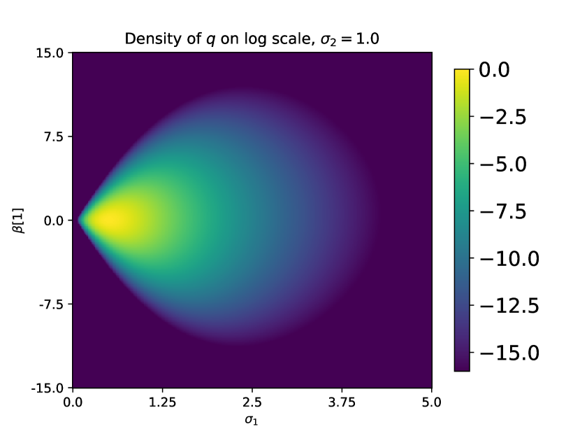
Figure 1: Density of $q$ (see (1)) with respect to $\sigma_{1}$ and $\beta_{1}$, where $\gamma=8$, $n=100$, $k=10$, and data were randomly generated.

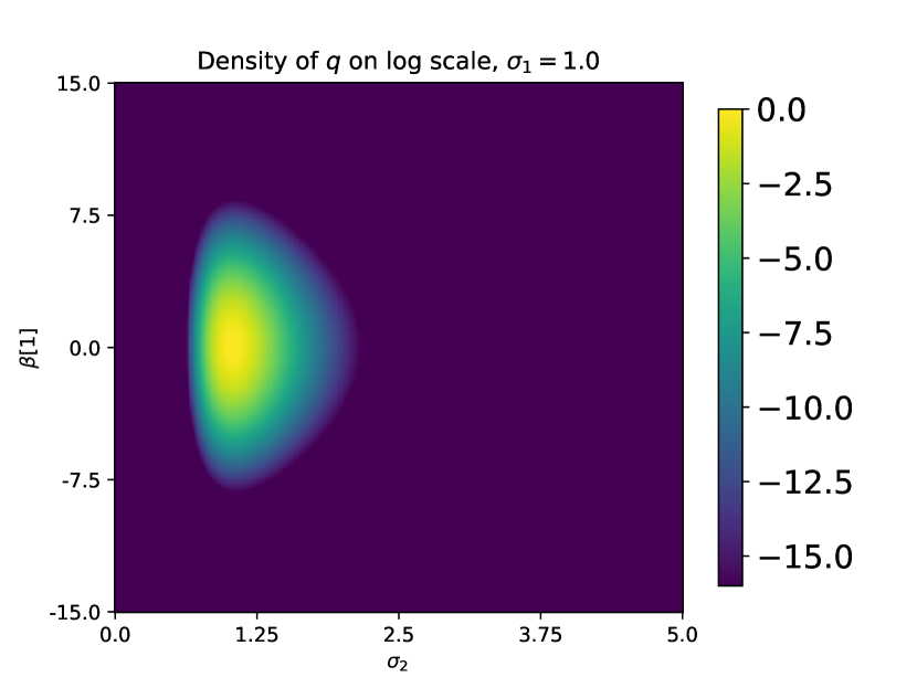
Figure 2: Density of $q$ (see (1)) with respect to $\sigma_{2}$ and $\beta_{1}$, for the same parameters as Figure 2.

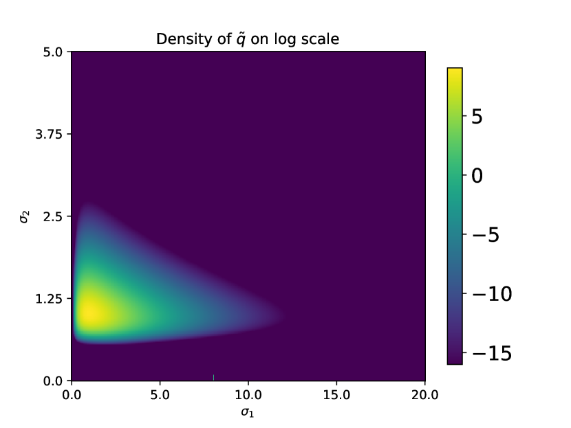
Figure 3: Density of $\tilde{q}$ (see (13)) using the same $q$ as Figure 2, where $n=100$, $k=10$, and data were randomly generated.

3 Evaluation of Posterior Means

Now that we have reduced the $k+2$-dimensional density $q$ to the $2$-dimensional density $\tilde{q}$, it remains to recover the posterior moments of $q$ using $\tilde{q}$. We first observe that moments of $\sigma_{1}$ and $\sigma_{2}$ with respect to $q$ are equivalent to moments of $\sigma_{1}$ and $\sigma_{2}$ over $\tilde{q}$. That is,

$$\mathbbm{E}_{q}(\sigma_{1})=\mathbbm{E}_{\tilde{q}}(\sigma_{1})$$ (14)

and

$$\mathbbm{E}_{q}(\sigma_{2})=\mathbbm{E}_{\tilde{q}}(\sigma_{2}).$$ (15)

As for moments of $\beta$, we use (13) and standard properties of Gaussians to obtain the following formula.

Formula 3.1.

For all $\sigma_{1},\sigma_{2}>0$,

$$\int_{\mathbbm{R}^{k}}z_{i}q(\sigma_{1},\sigma_{2},\beta)d\beta=\frac{a_{1,i}}{2a_{2,i}}\tilde{q}(t)$$ (16)

where $q$ is defined in (1), $\tilde{q}$ is defined in (13), $a_{2,i}$ is defined in (8), and $a_{1,i}$ is defined in (9).

As an immediate consequence of (16), we are able to evaluate the posterior expectation of $z$ as an expectation of a $2$-dimensional density:

$$\mathbbm{E}_{q}(z_{i})=\mathbbm{E}_{\tilde{q}}(\frac{a_{1,i}}{2a_{2,i}}).$$ (17)

We then transform those expectations back to expectations over the desired basis, $\beta$ using the matrix $V$ computed in (6). Specifically, using linearity of expectation and (17), we know

$$\begin{split}\mathbbm{E}_{q}((\beta_{1},\dots,\beta_{k})^{t})&=\mathbbm{E}_{q}(VV^{t}(\beta_{1},\dots,\beta_{k})^{t})\\ &=V\mathbbm{E}_{q}(V^{t}(\beta_{1},\dots,\beta_{k})^{t})\\ &=V\mathbbm{E}_{q}((z_{1},\dots,z_{k})^{t})\\ &=V\mathbbm{E}_{\tilde{q}}\left(\left(\frac{a_{1,1}}{2a_{2,1}},\dots,\frac{a_{1,k}}{2a_{2,k}}\right)^{t}\right).\end{split}$$ (18)

4 Covariance of $\beta$

In addition to facilitating the rapid evaluation of posterior means, the change of variables described in Section 2 is also useful for the evaluation of higher moments.

Equation (7) shows that after the change of variables from $\beta$ to $z$, the resulting density is a Gaussian in $z$ with a diagonal covariance matrix. Additionally, for each $z_{i}$, using equation (7) and standard properties of Gaussians, we have the following identity.

Formula 4.1.

For all $\sigma_{1},\sigma_{2}>0$, we have

$$\int_{\mathbbm{R}^{k}}(z_{i}-\mu_{z_{i}})^{2}q(\sigma_{1},\sigma_{2},\beta)d\beta=(2a_{2,i})^{-1}\tilde{q}(\sigma_{1},\sigma_{2})$$ (19)

where $\mu_{z_{i}}$ is the expectation of $z_{i}$, $\tilde{q}$ is defined in (13), and $a_{2,i}$ is defined in (8).

The second moments of the posterior of $\beta$ are obtained as a linear transformation of the posterior variances of $z$. In particular, denoting the expectation of $\beta$ by $\mu_{\beta}$ and the expectation of $z$ by $\mu_{z}$, we have

$$\begin{split}\mathbbm{E}((\beta-\mu_{\beta})(\beta-\mu_{\beta})^{t})&=VV^{t}\mathbbm{E}((\beta-\mu_{\beta})(\beta-\mu_{\beta})^{t})VV^{t}\\ &=V\mathbbm{E}(V^{t}(\beta-\mu_{\beta})(\beta-\mu_{\beta})^{t}V)V^{t}\\ &=V\mathbbm{E}((z-\mu_{z})(z-\mu_{z})^{t})V^{t}.\end{split}$$ (20)

We observe that due to the independence of all $z_{i}$,

$$\mathbbm{E}((z-\mu_{z})(z-\mu_{z})^{t})$$ (21)

is diagonal and we can therefore evaluate the $k\times k$ posterior covariance matrix of $\beta$ by evaluating $\mathrm{var}(z_{i})$ for $i=1,...,k$ and then applying two orthogonal matrices. Specifically, combining Formula 4.1 and (20), we obtain

$$\begin{split}\mathrm{cov}(\beta)&=V\mathbbm{E}_{\tilde{q}}\left(\left((2a_{2,1})^{-1},...,(2a_{2,k})^{-1}\right)^{t}\right)V^{t}.\end{split}$$ (22)

5 Variance of $\sigma_{1}$ and $\sigma_{2}$

Higher moments of $\sigma_{1}$ and $\sigma_{2}$ with respect to $q$ can be evaluated directly as higher moments of $\sigma_{1}$ and $\sigma_{2}$ with respect to $\tilde{q}$. That is, for all $j\in\{2,3,...,\}$, we have

$$\mathbbm{E}_{q}((\sigma_{1}-\mu_{\sigma_{1}})^{j})=\mathbbm{E}_{\tilde{q}}((\sigma_{1}-\mu_{\sigma_{1}})^{j})$$ (23)

and

$$\mathbbm{E}_{q}((\sigma_{2}-\mu_{\sigma_{2}})^{j})=\mathbbm{E}_{\tilde{q}}((\sigma_{2}-\mu_{\sigma_{2}})^{j}).$$ (24)

In particular, for $j=2$, we obtain

$$\mathrm{var}_{q}(\sigma_{1})=\mathrm{var}_{\tilde{q}}(\sigma_{1})$$ (25)

and

$$\mathrm{var}_{q}(\sigma_{2})=\mathrm{var}_{\tilde{q}}(\sigma_{2}).$$ (26)

1 Compute SVD of matrix $X$

2 Compute $w$ (see (11))

3 Compute $V^{t}\mathbbm{1}$ (see (9))

4 Construct evaluator for density $\tilde{q}$ of (13)

5 Evaluate first and second moments with respect to $\tilde{q}$: $\mathbbm{E}_{\tilde{q}}(\sigma_{1}),\mathbbm{E}_{\tilde{q}}(\sigma_{2}),\mathbbm{E}_{\tilde{q}}(\frac{a_{1,i}}{2a_{2,i}})$

6 Compute $\mathbbm{E}(\beta)$ via formula (18)

Algorithm 1 Evaluation of posterior expectations of normal-normal models

6 Numerical Experiments

Algorithm 1 was implemented in Fortran. We used the GFortran compiler on a 2.6 GHz 6-Core Intel Core i7 MacBook Pro. All examples were run in double precision arithmetic. The matrix $X$ and vector $y$ were randomly generated as follows. Each entry of $X$ was generated with an independent Gaussian with mean $0$ and variance $1$. The vector $y$ was created by first randomly generating a vector $\beta\in\mathbbm{R}^{k}$, each entry of which is an independent Gaussian with mean $0$ and variance $1$. The vector $y$ was set to the value of $X\beta+\epsilon$ where $\epsilon\in\mathbbm{R}^{n}$ contains standard normal iid entries. We generated $y$ this way in order to ensure that the $\mathbbm{E}(\beta_{i})$ were not all small in magnitude. We set $\gamma$ of (1) to 8.

In Table 2 and Figure 5, we compare the performance of Algorithm 1 to two alternative schemes for computing posterior expectations — one in which we analytically marginalize via equation (12) and then integrate the $2$-dimensional density via MCMC using Stan. In the other, we use Stan’s MCMC sampling on the full $k+2$ dimensional posterior. When using MCMC with Stan, we took 10,000 posterior draws. In Table 2 and Figure 5 we denote Algorithm 1 by “SVD-Trap”. The algorithm that uses Stan on the marginal $2$-dimensional density is labeled “SVD-MCMC”, and “MCMC” corresponds to the algorithm that uses only MCMC sampling in Stan.

In the appendix, we include Stan code to sample from the marginal density $\tilde{q}$ of (13).

Remark 6.1.

In the numerical integration stage of algorithm 1, we use the trapezoid rule with $200$ nodes in each direction. Because the integrand is smooth and vanishes near the boundary, convergence of the integral is super-algebraic when using the trapezoid rule (see [stoer]). A rectangular grid with $200$ points in each direction is satisfactory for obtaining approximately double precision accuracy. In problems with large numbers of non-normal-normal parameters, MCMC algorithms such as Hamiltonian Monte Carlo or other methods can be used.

In Tables 1 and 2, $n$ and $k$ represent the size of the $n\times k$ random matrix $X$.

The column labeled “max error” provides the maximum absolute error of the expectations of $\sigma_{1}$, $\sigma_{2}$, and $\beta_{i}$ for $i\in\{1,2,\dots,n\}$. The true solution was evaluated using trapezoid rule with $500$ nodes in each direction in extended precision.

In Table 1, “Precompute time (s)” denotes the time in seconds of all computations until numerical integration. These times are dominated by the cost of SVD (28). The total time of the numerical integration in addition to the matrix-vector product (18) is given in “integrate time (s).” The final column of Table 1, “total time (s)”, provides the total time of precomputation and integration.

$n$	$k$	max error	precompute time (s)	integrate time (s)	total (s)
$50$	$5$	$0.22\times 10^{-13}$	$0.01$	$0.01$	0.02
$100$	$10$	$0.26\times 10^{-13}$	$0.02$	$0.01$	0.03
$500$	$20$	$0.30\times 10^{-13}$	$0.04$	$0.01$	0.05
$1000$	$50$	$0.34\times 10^{-13}$	$0.09$	$0.03$	0.12
$5000$	$100$	$0.37\times 10^{-13}$	$0.29$	$0.05$	0.34
$10000$	$500$	$0.26\times 10^{-13}$	$14$	$0.3$	14.2
$10000$	$1000$	$0.39\times 10^{-13}$	$54$	$0.6$	54.5

Table 1: Scaling of computation times for evaluation of expectations of $q$ (see (1)) using Algorithm 1

Figure 4: Scaling of computation times for evaluation of posterior expectations of $q$ (see (1)) using Algorithm 1 as a function of $k$ with $n=10,000$.

		SVD-Trap		SVD-MCMC		MCMC
$n$	$k$	time (s)	error	time (s)	error	time (s)	error
$100$	$100$	$0.16$	$0.9\times 10^{-14}$	$11$	$0.4\times 10^{-4}$	$16$	$0.1\times 10^{-1}$
$200$	$100$	$0.16$	$0.9\times 10^{-14}$	$11$	$0.3\times 10^{-2}$	$24$	$0.8\times 10^{-2}$
$500$	$100$	$0.23$	$0.9\times 10^{-13}$	$12$	$0.2\times 10^{-2}$	$40$	$0.8\times 10^{-2}$
$1000$	$100$	$0.25$	$0.2\times 10^{-13}$	$12$	$0.6\times 10^{-3}$	$88$	$0.7\times 10^{-2}$
$5000$	$100$	$0.30$	$0.4\times 10^{-13}$	$14$	$0.2\times 10^{-3}$	$617$	$0.3\times 10^{-2}$
$10000$	$100$	$0.65$	$0.2\times 10^{-13}$	$13$	$0.4\times 10^{-3}$	$2552$	$0.2\times 10^{-2}$

Table 2: Scaling of computation times for evaluation of expectations of $q$ (see (1)) using three different algorithms: i) SVD-Trap: Algorithm 1 of this paper, ii) SVD-MCMC: marginalization with MCMC integration of $\tilde{q}$ using Stan, and iii) MCMC: full MCMC integration of $q$ using Stan.

Figure 5: Scaling of computation times for evaluation of posterior expectations of $q$ (see (1)) as a function of sample size $n$ with $k=100$. The three algorithms comapred are i) SVD-Trap: Algorithm 1 of this paper, ii) SVD-MCMC: marginalization with MCMC integration of $\tilde{q}$ using Stan, and iii) MCMC: full MCMC integration of $q$ using Stan.

7 Generalizations and Conclusions

In this paper, we present a numerical scheme for the evaluation of the expectations of a particular class of distributions that appear in Bayesian statistics; posterior dsitributions of linear regression problems with normal-normal parameters.

The scheme presented generalizes naturally to several classes of distributions that appear frequently in Bayesian statistics. We list several examples of posteriors whose expectations can be evaluated using this method.

1. The choice of priors for $\sigma_{1}$, and $\sigma_{2}$ in this document were log normal and half-normal. This choice did not substantially impact the algorithm and can be generalized. Adaptive Gaussian quadrature can be used for the numerical integration step of the algorithm for a more general choice of prior on $\sigma_{1}$ and $\sigma_{2}$.

2. Multilevel regression problems with more than two levels.

3. Regression problems with multiple groups such as the two-group model with posterior exp( -12σ12 ∥Xβ- y∥^2 - 12σ22∑_i=1^k_1 (μ_1 - β_i)^2 - 12σ32∑_i=k_1 + 1^k_1 + k_2 β_i^2 ) where $X$ is a $n\times k$ matrix, $y\in\mathbbm{R}^{n}$, and $k_{1}$ and $k_{2}$ are non-negative integers satisfying $k_{1}+k_{2}=k$.
3. Regression problems with correlated priors on $\beta$: exp( -12σ22 ∥X_1β- y∥^2 - 12σ12∥X_2 β∥ ) For regression problems with large numbers of non-normal-normal parameters, marginal expectations can be computed using, for example, MCMC in Stan. For such problems, the algorithm of this paper would convert an MCMC evaluation from $k+m$ dimensions to $m$ dimensions, where $k$ is the number of normal-normal parameters.

8 Acknowledgements

The authors are grateful to Ben Bales and Mitzi Morris for useful discussions.

Appendix A Code

The following Stan code allows for sampling from the distribution corresponding to the probability density function proportional to (1).

data {
  int n;
  int k;
  vector[n] y;
  matrix[n,k] X;
}
parameters {
  real<lower=0> sigma1;
  real<lower=0> sigma2;
  vector<offset=0, multiplier=sigma1>[k] beta;
}
model {
  y ~ normal(X*beta, sigma2);
  beta ~ normal(0, sigma1);
  sigma1 ~ lognormal(0, 0.25);
  sigma2 ~ normal(0, 1);
}

The following Stan program samples from the marginal density $\tilde{q}$ (see (13)). The data input yty corresponds to $y^{t}y$ of (10), lam is the vector of singular values of $X$, and w is the vector $w$ in equation (11). We include R code for computing yty, lam, and w after the following Stan code.

functions {
  real q_tilde_lpdf(real sig1, real sig2, vector w, vector lam, real yty,
                    int k, int n) {
    vector[min(n,k)] a2 = lam^2/(sig2^2) + 1/(sig1^2);
    real sol = sum(w^2 ./a2)/2/sig2^4 - sum(log(a2))/2 -yty/(2*sig2^2);
    sol += -min(n,k)*log(sig1) - n*log(sig2);
    return sol;
  }
}
data {
  int n;
  int k;
  vector[min(n,k)] w;
  vector[min(n,k)] lam;
  real yty;
  matrix[min(n,k),k] V;
}
parameters {
  real<lower=0> sigma1;
  real<lower=0> sigma2;
}
model {
  sigma1 ~ q_tilde(sigma2, w, lam, yty, k, n);
  sigma1 ~ lognormal(0, 0.25);
  sigma2 ~ normal(0, 1);
}
generated quantities {
 vector[k] beta;
 {
   vector[min(n,k)] zvar = 1 ./(2*(lam^2 ./(2*sigma2^2) + 1/(2*sigma1^2)));
   vector[min(n,k)] zmu = w./sigma2^2 .* zvar;
   vector[min(n,k)] z = to_vector(normal_rng(zmu, sqrt(zvar)));
   beta = V * z;
 }
}

The following is a sample of code from R that can be used for the precomputation stage of Algorithm 1.

udv <- svd(X)
V <- udv$v
lam <- as.vector(udv$d)
w <- t(V) %*% t(X) %*% y
w <- as.vector(w)
yty <- t(y) %*% y
yty <- yty[1]

Appendix B Proofs

In this appendix, we include proofs of the formulas provided in this paper. For increased readability, this appendix is self-contained.

B.1 Mathematical Preliminaries and Notation

In this section, we introduce notation and elementary mathematical identities that will be used throughout the remainder of this section. We define $C\in\mathbbm{R}$ by the equation

$$C=\int_{\sigma_{1}\in\mathbbm{R}^{+}}\int_{\sigma_{2}\in\mathbbm{R}^{+}}\int_{\beta\in\mathbbm{R}^{k}}q(\sigma_{1},\sigma_{2},\beta)d\beta d\sigma_{2}d\sigma_{1},$$ (27)

and define $\mathbbm{E}(\sigma_{1})$, $\mathbbm{E}(\sigma_{2})$, and $\mathbbm{E}(\beta_{i})$ by the formulas E(σ_1) = 1C ∫_σ_1∈R^+ ∫_σ_2∈R^+ ∫_β∈R^k σ_1 q(σ_1, σ_2, β) dβdσ_2 dσ_1, E(σ_2) = 1C ∫_σ_1∈R^+ ∫_σ_2∈R^+ ∫_β∈R^k σ_2 q(σ_1, σ_2, β) dβdσ_2 dσ_1, and E(β_i) = 1C ∫_σ_1∈R^+ ∫_σ_2∈R^+ ∫_β∈R^k β_i q(σ_1, σ_2, β) dβdσ_2 dσ_1 for $i\in\{1,2,\dots,k\}$. We provide algorithms for the evaluation of (27), (27), (27), and (27). We will be denoting by $\mathbbm{1}$ the vector of ones 1 = (1,1,…,1)^t. We denote the $i^{th}$ component of a vector $v$ by $v_{i}$. The following two well-known identities give the normalizing constant and expectation of a Gaussian distribution.

Lemma B.1.

For all $\sigma_{1},\sigma_{2}>0$ we have 2πσ= ∫_R e^-(β- μ)22σ2dβ

Lemma B.2.

For all $\mu$ in $\mathbbm{R}$ and $\sigma>0$, we have μ2πσ= ∫_R βe^-(β- μ)22σ2dβ

B.2 Analytic Integration of $\beta$

We denote the singular value decomposition of $X$ by

$$X=UDV^{t}$$ (28)

where $U$ is an orthogonal $n\times k$ matrix, $V$ is an orthogonal $k\times k$ matrix, and $D$ is a $k\times k$ diagonal matrix. We define $z\in\mathbbm{R}^{k}$ by the formula z = V^tβ. The following lemma, which will be used in the proof of Lemma LABEL:170, gives an expression for the second to last term of the exponent in (1) after a change of variables.

Lemma B.3.

For all $\beta\in\mathbbm{R}^{k}$, and $y\in\mathbbm{R}^{n}$, -12σ22∥ Xβ- y∥^2 = -yty2σ22 + ∑_i=1^k -λi22σ22 z_i^2 + wiσ22z_i

where w = V^tX^ty, $z$ is defined in (28), and $\lambda_{i}$ is the $i^{th}$ entry on the diagonal of $D$ (see (28)). Proof. Clearly, ∥Xβ- y∥^2 = β^tX^tXβ- 2y