Direct Numerical Simulations of the Swirling von Kármán Flow Using a Semi-implicit Moving Immersed Boundary Method

Abstract

We present a novel moving immersed boundary method (IBM) and employ it in direct numerical simulations (DNS) of the closed-vessel swirling von Kármán flow in laminar and turbulent regimes. The IBM extends direct-forcing approaches by leveraging a time integration scheme, that embeds the immersed boundary forcing step within a semi-implicit iterative Crank-Nicolson scheme. The overall method is robust, stable, and yields excellent results in canonical cases with static and moving boundaries. The moving IBM allows us to reproduce the geometry and parameters of the swirling von Kármán flow experiments in (F. Ravelet, A. Chiffaudel, and F. Daviaud, JFM 601, 339 (2008)) on a Cartesian grid. In these DNS, the flow is driven by two-counter rotating impellers fitted with curved inertial stirrers. We analyze the transition from laminar to turbulent flow by increasing the rotation rate of the counter-rotating impellers to attain the four Reynolds numbers 90, 360, 2000, and 4000. In the laminar regime at Reynolds number 90 and 360, we observe flow features similar to those reported in the experiments and in particular, the appearance of a symmetry-breaking instability at Reynolds number 360. We observe transitional turbulence at Reynolds number 2000. Fully developed turbulence is achieved at Reynolds number 4000. Non-dimensional torque computed from simulations matches correlations from experimental data. The low Reynolds number symmetries, lost with increasing Reynolds number, are recovered in the mean flow in the fully developed turbulent regime, where we observe two tori symmetrical about the mid-height plane. We note that turbulent fluctuations in the central region of the device remain anisotropic even at the highest Reynolds number 4000, suggesting that isotropization requires significantly higher Reynolds numbers.

1 Introduction

Engineering flows operated in closed vessels, such as internal combustion engines and stirred tank reactors, are often subject to high levels of shear and velocity fluctuations. In these flows, the interaction between moving surfaces and the flow controls macroscopic quantities such as mixing rates and power consumption (Bertrand et al., 1980). In the present paper, we develop a moving immersed boundary (IB) strategy that enables the study of highly turbulent flows interacting with moving components. We validate the method in canonical cases then apply it in direct numerical simulations (DNS) of the inertially-driven swirling von Kármán flow, a closed vessel flow of fundamental and practical interest. We show that laminar and turbulent regimes of the swirling von Kármán flow can be reproduced successfully by DNS with our IB method and analyze the homogeneity and anisotropy of the flow in the fully developed turbulence regime.

Owing to its fundamental nature, the swirling von Kármán flow received significant attention. In his pioneering work, Theodor von Kármán (Kármán, 1921) considered the flow over an infinite disk rotating at a rate $\Omega$. Von Kármán noted that the flow is self-similar and that the Navier-Stokes equations may be reduced to a pair of non-linear ordinary differential equations. Batchelor (1951) further generalized the analysis to include a second coaxial disk at a distance $H$. The solution to these equations is chaotic and offers key insights into the non-linearity of the Navier Stokes equations. The earlier work of von Kármán and Batchelor was followed by sustained research efforts to analyze the flow characteristics in various regimes (see review of Zandbergen and Dijkstra (1987)). More recently, the case of counter-rotating finite disks of radius $R$ received significant attention. While the flow is characterized by symmetry at low Reynolds number $\mbox{Re}_{\Omega}$, several authors reported the appearance of symmetry-breaking hydrodynamic instabilities with increasing $\mbox{Re}_{\Omega}$ (Lopez et al., 2002; Nore et al., 2003, 2004; Cortet et al., 2011). Here, the Reynolds number is defined as $\mbox{Re}_{\Omega}=\Omega R^{2}/\nu$, where $\nu$ is the kinematic viscosity. The resulting flow structures are stable and persist for a wide range of intermediate Reynolds numbers before the onset of additional symmetry-breaking instabilities (Ravelet, 2005; Ravelet et al., 2008). At large Reynolds numbers, a turbulent shear layer forms between two stacked toroidal cells of size comparable to the disk diameter.

From an experimental perspective, the case of counter-rotating disks is of particular interest as it produces high Reynolds number turbulence inside a closed and compact device. Maurer et al. (1994) produced a turbulent von Kármán flow with Taylor micro-scale Reynolds number $\mbox{Re}_{\lambda}\sim 2100$ in a device of disk radius and separation $R=3.2\,\mbox{cm}$ and $H=4.8\,\mbox{cm}$, respectively. Odier et al. (1998) achieved a macroscopic Reynolds number $\mbox{Re}_{\Omega}=\Omega R^{2}/\nu=O(10^{6})$ with $R=H=10\,\mbox{cm}$. Curved inertial-stirrers mounted on the disks increase velocity fluctuations and are used to tune flow structures (Ravelet et al., 2005; Ravelet, 2005; Burnishev and Steinberg, 2014). Access to such high Reynolds number regimes enables studies of fundamental turbulence properties such as intermittency, energy dissipation, and the turbulence cascade (Monchaux et al., 2008; Debue et al., 2018; Dubrulle, 2019; Kuzzay et al., 2015).

Further work on the fine scale structures of the von Kármán flow requires spatial and temporal resolutions for which numerical studies are in principle better suited. Unlike the vigorous experimental effort deployed so far, investigations of the von Kármán flow relying on direct numerical simulations remain scarce. Few studies resolved the flow around the blades (Kreuzahler et al., 2014; Nore et al., 2018). While the existence of numerous experimental data sets enables insightful comparisons between experiments and simulations, it remains to be shown that current numerical methods are able to reproduce experimental findings. Addressing this issue requires a computational strategy that manages computational cost while ensuring an accurate representation of the flow near the impellers.

Immersed boundary (IB) methods are a natural choice for simulations that involve complex geometries, such as the inertially-driven swirling von Kármán flow. These methods remove the cumbersome task of generating body-conformal meshes and enable the use of straightforward Cartesian grids for the discretization of the volume occupied by the fluid. Various approaches are summarized in (Mittal and Iaccarino, 2005). The so-called direct-forcing IB method (Peskin, 1972) relies on a forcing term added to the right hand-side of the momentum equation in order to impose no-slip boundary conditions. This class of methods is amenable to efficient discretization and can handle moving immersed boundaries robustly (Roma et al., 1999; Peskin, 2002; Lai and Peskin, 2000). Since the original work of Peskin, various improvements have been proposed (Fadlun et al., 2000; Kim et al., 2001; Balaras, 2004; Kim and Choi, 2006; Nicolaou et al., 2015; Kang et al., 2009). In particular, Uhlmann (2005) proposed that the forcing be applied on Lagrangian points distributed on the surface of the immersed solid. This method is characterized by its robustness and stability. Variations of Uhlmann’s Lagrangian direct-forcing method have been proposed (Yang and Balaras, 2006; Vanella and Balaras, 2009).

In the present work, we conduct DNS of the swirling von Kármán flows using a novel moving IB method derived from Uhlmann (2005)’s method. First, we show that the properties of the Lagrangian markers (position and size) can be obtained from a triangular tessellation of the IB surface. Second, we couple the IB forcing to the update of the velocity and pressure fields by means of operator-splitting within a semi-implicit iterative Crank-Nicolson scheme for the advancement of momentum in incompressible flows (Pierce, 2001; Pierce and Moin, 2004; Choi and Moin, 1994). The overall scheme allows a rapid workflow, whereby a mesh of the von Kármán flow enclosure and impellers generated by a CAD software is loaded in a direct numerical simulation flow solver without further adjustment. Data generated with this approach is compared to the experiments of Ravelet et al. (2008) in the laminar and turbulent regimes.

The paper is organized as follows. The governing equations and numerical discretization are introduced in Section 2. In Section 3, we validate the method in three benchmark cases including static and moving IBs. Simulations of the inertially-driven swirling von Kármán flow are presented in Section 4. Two laminar cases at $\mbox{Re}_{\Omega}=90$ and $\mbox{Re}_{\Omega}=365$ are considered in Section 4.1. Two additional cases at $\mbox{Re}_{\Omega}=2000$ and $\mbox{Re}_{\Omega}=4000$ are considered in Sections 4.2. Final remarks are given in Section 5.

2 Equations and methods

2.1 Governing equations

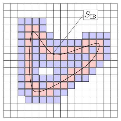
Figure 1: No-slip boundary conditions on an immersed solid are enforced using a forcing term applied to the right hand-side of the momentum equation. To maintain a sharp representation of the interface, the term has a compact support of three mesh widths applied to the cut-cells (red) and closest neighbors (blue).

Consider a solid with boundary surface $S_{\mathrm{IB}}$ immersed in an incompressible fluid of density $\rho$ and viscosity $\mu$. The fluid obeys mass and momentum conservation equations

$$\nabla\cdot\bm{u} = 0$$ (1)

$$\rho\left(\frac{\partial\bm{u}}{\partial t}+\bm{u}\cdot\nabla\bm{u}\right) = -\nabla p+\mu\nabla^{2}\bm{u}+\bm{F}_{\mathrm{IB}},$$ (2)

where $\bm{u}$ is the fluid velocity and $p$ is the pressure. In the direct-forcing approach (Peskin, 1972, 2002), the IB forcing term

$$\bm{F}_{\mathrm{IB}}(\bm{x},t)=\iint_{\bm{y}\in S_{\mathrm{IB}}}\bm{f}_{\mathrm{IB}}(\bm{y},t)\delta(\bm{x}-\bm{y})dS$$ (3)

enforces no-slip boundary conditions on the surface of the immersed solid. The field $\bm{f}_{\mathrm{IB}}$ represents the Lagrangian forcing at a location $\bm{y}$ belonging to the immersed surface $S_{\mathrm{IB}}$. Multiple immersed bodies are addressed by splitting $S_{\mathrm{IB}}$ into an arbitrary number of sets.

In addition to (1) and (2), additional equations describing the motion of the solid may be added and coupled to the governing equations for the fluid. The IB forcing term (3) provides the coupling force between the immersed solid and the fluid. In the present work, we consider immersed solids with a prescribed rigid body motion.

2.2 Overview of the algorithm

Figure 2: Algorithm flow chart showing the successive momentum, IB and pressure steps. The time integration relies on a semi-implicit iterative crank-Nicolson scheme and operator splitting.

The governing equations are discretized and solved by the massively-parallel code NGA (Desjardins et al., 2008). The algorithm is shown in Fig 2. The immersed boundary is discretized using a tessellation of $N$ triangular facets $S_{m}$, such that $S_{\mathrm{IB}}=\cup_{m=1}^{N}S_{m}$. At the beginning of each time step, the position of the immersed boundary is updated by moving the centroids of the triangles from their previous locations $\bm{x}^{n}_{m}$ to new positions $\bm{x}^{n+1}_{m}$ according to the prescribed rigid body motion.

Next, the velocity field is updated while enforcing mass conservation. The time integration scheme for the momentum and pressure relies on the semi-implicit iterative Crank-Nicolson scheme introduced by (Akselvoll, 1995) and further developed in (Pierce, 2001; Pierce and Moin, 2004). We use an operator splitting approach to update the momentum and pressure, while considering the effects of the immersed solids, in three consecutive updates.

Consider the $(k+1)^{\mathrm{th}}$ sub-iteration. First, we perform a conventional momentum update, where the IB forcing term and pressure term are omitted. The update reads

$$\tilde{\bm{u}}^{n+1}_{k+1}=\bm{u}^{n}+\Delta t\mathcal{M}(\bm{u}^{n+1/2}_{k+1})+\Delta t\frac{\partial\mathcal{M}}{\partial\bm{u}}\left(\frac{\tilde{\bm{u}}^{n+1}_{k+1}-\bm{u}^{n+1}_{k}}{2}\right).$$ (4)

In the above, the mid-step velocity is $\bm{u}^{n+1/2}_{k+1}=(\bm{u}^{n}+\bm{u}^{n+1}_{k})/2$ and $\mathcal{M}$ is the operator comprising both convective and viscous terms

$$\mathcal{M}(\bm{u})=-\nabla\cdot(\bm{u}\bm{u})+\frac{\mu}{\rho}\nabla^{2}\bm{u}.$$ (5)

The Jacobian $\partial M/\partial\bm{u}$ in equation (4) allows the treatment of the non-linearity with a Newton-Raphson method (Pierce, 2001). The momentum equation is solved with the approximate factorization technique of Choi and Moin (1994) based on the Alternating Direction Implicit (ADI) method. The method conserves mass, momentum and kinetic energy discretely (Pierce, 2001; Desjardins et al., 2008; Choi and Moin, 1994).

Next, the velocity is updated by applying the IB forcing

$$\hat{\bm{u}}^{n+1}_{k+1}=\tilde{\bm{u}}^{n+1}_{k+1}+\Delta t\bm{F}^{n+1}_{\mathrm{IB},k+1}/\rho.$$ (6)

Lastly, a pressure-projection step is performed to enforce continuity by solving a Poisson equation and later correcting the velocity

$$\nabla^{2}p^{n+1}_{k+1} = \rho\frac{\nabla\cdot\hat{\bm{u}}^{n+1}_{k+1}}{\Delta t},$$ (7)

$$\bm{u}_{k+1}^{n+1} = \hat{\bm{u}}^{n+1}_{k+1}-\frac{\Delta t}{\rho}\nabla p^{n+1}_{k+1}.$$ (8)

These sub-iterations are embedded within the iterative Crank-Nicolson loop. Typically, two to three subiterations per time step are used (Pierce, 2001). Note that if the Jacobian term is omitted and only two sub-iterations are retained, the time discretization becomes equivalent to an explicit second order Runge-Kutta scheme.

2.3 Treatment of the immersed boundaries

We now focus on the discretization of the forcing term in equation (6). Since $S_{\mathrm{IB}}=\cup_{m=1}^{N}S_{m}$, the forcing can be written as the sum of discrete contributions

$$\bm{F}^{n+1}_{\mathrm{IB},k+1}(\bm{x})=\sum_{m=1}^{N}\iint_{\bm{y}\in S_{m}}\bm{f}^{n+1}_{\mathrm{IB},k+1}(\bm{y})\delta_{h}(\bm{x}-\bm{y})dS,$$ (9)

where, in the actual implementation, the Dirac delta is replaced by a regularized delta of finite width $h$ (Peskin, 2002). Note that, in this approach, internal cells are not forced. The integrals on the facets are approximated to second-order accuracy using the mid-point rule

$$\bm{F}^{n+1}_{\mathrm{IB},k+1}(\bm{x})=\sum_{m=1}^{N}\bm{f}^{n+1}_{m,k+1}\delta_{h}(\bm{x}-\bm{x}_{m})A_{m},$$ (10)

where $A_{m}$ is the surface area of facet $S_{m}$ and $\bm{f}^{n+1}_{m,k+1}$ is the Lagrangian IB forcing at the centroid $\bm{x}_{m}^{n+1}$. Following Uhlmann (2005), no-slip boundary conditions are enforced on the immersed surface $S_{\mathrm{IB}}$ by ensuring that the fluid velocity equals the IB velocity $\bm{u}_{\mathrm{IB},m}$ at the centroid $\bm{x}_{m}$. This yields the following Lagrangian forcing terms

$$\bm{f}^{n+1}_{m,k+1}=\rho h\frac{\bm{u}^{n+1}_{\mathrm{IB},m}-\tilde{\bm{u}}^{n+1}_{k+1}(\bm{x}_{m})}{\Delta t}.$$ (11)

Thus, the resulting Eulerian forcing term in (6) reads

$$\bm{F}^{n+1}_{\mathrm{IB},k+1}=\sum_{m=1}^{N}\rho\left(\frac{\bm{u}^{n+1}_{\mathrm{IB},m}-\tilde{\bm{u}}^{n+1}_{k+1}(\bm{x}_{m})}{\Delta t}\right)\delta_{h}(\bm{x}-\bm{x}_{m})hA_{m}.$$ (12)

The fluid velocity at the centroids is obtained by interpolation from neighboring nodes on the Eulerian grid with $\delta_{h}$ as interpolation kernel. Here, we use the regularized Dirac delta proposed by Roma et al. (1999), which has a compact support of width $h$. By choosing $h=3\Delta x$, where $\Delta x$ is the homogeneous mesh spacing, we ensure a sharp representation of the IB and efficient summation in (12).

3 Validation cases

In this section, we evaluate the accuracy and performance of the IB method against experimental and numerical data in canonical laminar flows. Three cases are discussed: the flow around a static cylinder placed asymmetrically in a channel, the flow around a static cylinder in free stream, and the flow around a transversely oscillating cylinder.

3.1 Static cylinder placed asymmetrically in a channel

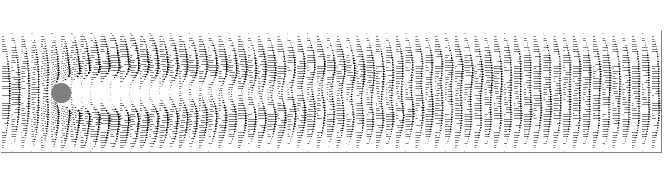
(a) Vortex shedding in the wake of an asymmetrically placed cylinder.

(b) Drag coefficient

(c) Lift coefficient

Figure 3: Flow past an asymmetrically placed cylinder at $\mbox{Re}=100$. Data for $D/\Delta x=48.8$ and $\mathrm{CFL}_{\mathrm{max}}\sim 0.25$.

Table 1: Strouhal number, drag and lift coefficients for the case of a cylinder placed asymmetrically in a channel at $\mbox{Re}=100$.

	$D/\Delta x$	St	$C_{D,max}$	$C_{L,max}$
present	24.4	0.308	3.544	0.783
present	48.8	0.306	3.575	0.886
present	97.6	0.303	3.442	0.907
Schäfer et al. (1996)	-	$0.3\pm 0.005$	$3.23\pm 0.01$	$1.0\pm 0.01$

We first consider the two-dimensional configuration in the benchmark flow of Schäfer et al. (1996). A cylinder of diameter $D$ is placed in a channel of height $H=4.1D$ and length $L=22D$. The static cylinder is placed asymmetrically at $x=y=0.3$. A parabolic inflow with average velocity $U$ is prescribed at the inlet $x=0$. The fluid kinematic viscosity $\nu$ is such that $\mbox{Re}_{D}=UD/\nu=100$. Three spatial resolutions are considered where $D/\Delta x$ equals 24.4, 48.8 and 97.6, respectively. In all configurations, the maximum Courant–Friedrichs–Lewy number $\mathrm{CFL}$ is $\sim 0.25$.

The flow around the cylinder results in an oscillating wake, as shown in Fig. 3(a). Vortex shedding leads to fluctuating drag and lift coefficients as in Fig. 3(b) and 3(c). Once a stationary state sets in after $tU/D\sim 200$, we collect statistics from the time histories of drag and lift forces.

Comparison with the data in Schäfer et al. (1996) is shown in Tab. 1. We report the Strouhal number, maximum drag coefficient and maximum lift coefficient for increasing resolution from $D/\Delta x=24.4$ to $97.6$. For the case with the highest resolution, the shedding frequency $f_{0}$ yields a characteristic Strouhal number $\mbox{St}=f_{0}D/U\sim 0.303$ well within the range $0.295-0.305$ in (Schäfer et al., 1996). The maximum drag coefficient and maximum lift coefficient fall within 7% and 0.6% of the values reported in the literature, respectively.

3.2 Static cylinder in uniform crossflow

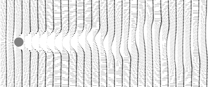
(a) Vortex street behind an immersed cylinder at $\mbox{Re}_{D}=100$.

(b) Drag coefficient

(c) Lift coefficient

Figure 4: Drag and lift coefficients over an immersed cylinder in a uniform free stream at $\mbox{Re}_{D}=100$. Data for $D/\Delta x=48.8$ and $\mathrm{CFL}\sim 0.25$.

Table 2: Strouhal number, drag and lift coefficients for the case of a cylinder in free stream at $\mbox{Re}=100$.

	$D/\Delta x$	St	$\bar{C}_{D}$	$C^{\prime}_{D}$	$C^{\prime}_{L}$
Present	24.4	0.167	1.500	0.004	0.250
Present	48.8	0.167	1.526	0.005	0.289
Present	97.6	0.167	1.531	0.007	0.299
Liu et al. (1998)	–	0.165	1.350	0.012	0.339
Williamson (1989)	–	0.164	–	–	–

Next, we consider a static cylinder of diameter $D=0.3$ placed in free stream with uniform inlet velocity. The computational domain has a size $26D\times 26D$. The cylinder is located at $x_{c}=6D$ and $y_{c}=4D$ from the bottom left corner. A uniform free-stream velocity $u_{\infty}=1$ is prescribed at the left inlet boundary, and convective outflow conditions are applied to the remaining boundaries. The Reynolds number is $\mbox{Re}_{D}=u_{\infty}D/\nu=100$. The domain is discretized on a uniform grid of size $128^{2}$, $256^{2}$ or $512^{2}$. The resulting resolution is $D/\Delta x=24.4$, 48.8 and 97.6. Note that the timestep $\Delta t$ is also adjusted to maintain $\mathrm{CFL}$ approximately constant at $0.25$.

Figure 4(a) shows the vortex street created by the immersed cylinder. The vortices are shed from the top and bottom sides of the cylinder at a natural frequency $f_{0}$. We obtain a Strouhal number $\mbox{St}=f_{0}D/u_{\infty}=0.167$ sensitively close to $0.164$ and $0.165$ determined from the experiments of Williamson (1989) and body-fitted simulations of Liu et al. (1998),respectively.

Figure 4(b) and 4(c) show the time history of drag and lift coefficients. For the runs with highest resolution $D/\Delta x=97.6$, we find an average $C_{D}=1.531$ and a root mean square (rms) fluctuation $C^{\prime}_{D}=0.007$. The mean lift coefficient is vanishingly small, as expected, while the fluctuation is $C^{\prime}_{L}=0.299$. These values are compared with those in (Liu et al., 1998) and shown in Tab 2. We note that there is an over-prediction of the drag coefficient by 13% and under-prediction of the rms lift coefficient by 12%. This behavior is similar to the observations of Uhlmann (2005), from which the method is derived.

3.3 Cylinder oscillating transversely in free stream

(a)

(b)

Figure 5: Drag coefficient for a transversely oscillating cylinder in free stream at $\mbox{Re}=185$. Data for $D/\Delta x=48.8$ and $\Delta tD/U_{\mathrm{max}}=0.0025$

Table 3: Strouhal number, drag and lift coefficients for the case of a cylinder oscillating transversely at $\mbox{Re}=185$ and $f_{e}/f_{0}=0.8$.

	$\Delta tU_{\mathrm{max}}/D$	$\bar{C}_{D}$	$C^{\prime}_{D}$
Present	0.0100	1.490	0.048
Present	0.0050	1.394	0.047
Present	0.0025	1.323	0.044
Lu and Dalton (1996)	–	1.25	–

The configuration described in the previous section is now modified to allow oscillations of the cylinder. The latter moves transversely whereby the displacement of the center is given by $\Delta y_{c}=0.2D\sin(2\pi f_{e}t)$. The forcing oscillation frequency is $f_{e}=0.8f_{0}$, where $f_{0}$ is the natural shedding frequency for a fixed cylinder at Reynolds number $\mbox{Re}=185$. These parameters follow the simulations in (Lu and Dalton, 1996) using a body-fitted method. For this case, we maintain a fixed spatial resolution at $512\times 512$, giving a ratio $D/\Delta x=48.8$, while the timestep $\Delta t$ is set at $0.01U_{\mathrm{max}}/D$, $0.005U_{\mathrm{max}}/D$, or $0.0025U_{\mathrm{max}}/D$. The corresponding $\mathrm{CFL}$ is 0.5,0.25, and 0.125, respectively.

Figure 5 shows the evolution of the drag coefficient for the case with $\Delta t=0.0025U_{\mathrm{max}}/D$. As seen in 5(a), the drag coefficient reaches a stationary state after approximately $130D/U$. For the case where $\Delta t=0.0025U/D$, the average drag coefficient (see Tab. 3) is within 6% of the value reported by Lu and Dalton (1996). The drag curve plotted as a function of displacement in 5(b) follows a figure eight shape similar to the one found in (Uhlmann, 2005). We note the presence of spurious oscillations in Fig. 5(b) that increase the rms drag coefficient fluctuations. As argued in (Uhlmann, 2005), these spurious oscillations can be reduced with larger discrete Dirac delta support than considered here.

4 The swirling von Kármán flow

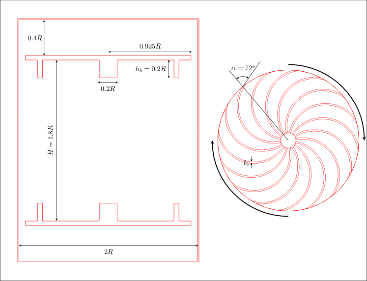
Figure 6: Geometry of the device. The top and bottom disks rotate in opposite directions at a constant rotation rate. The impeller design corresponds to the configuration TM60 analyzed in (Ravelet et al., 2008).

We now apply the immersed boundary method described in Section 2 to simulations of the swirling von Kármán flow.

The von Kármán flow considered in our work is generated in a closed cylindrical vessel between two counter-rotating disks fitted with curved blades as shown in Fig. 6. The numerical setup is a reproduction of the experimental apparatus analyzed by Ravelet et al. (2008) given available information in (Ravelet et al., 2008; Ravelet, 2005). The disks have radius equal to $0.925R$, where $R$ is the inner cylinder’s radius, and separation $H=1.8R$. The impellers act as centrifugal pumps that ingest fluid along the centerline and expel it radially towards the cylindrical walls. Inertial stirring is aided by 16 blades mounted on the disks. The stirrers correspond to the TM60 design in (Ravelet, 2005). They have a height $h_{b}=0.2R$, a thickness $t_{b}=0.02R$, and radius of curvature $C=R/(2\mbox{sin}\alpha)$, where the curvature angle is $\alpha=72^{\circ}$. All 16 blades are connected to a cylindrical hub of radius $0.1R$ and height equal to that of the blades. Flow ejected towards the walls by the impellers may enter a recirculation regions behind the disks of height $0.4R$.

Table 4: Simulation parameters for the five cases at $\mbox{Re}_{\Omega}=90$, 360, 2000 and 4000.

		laminar			turbulent
Parameter	Symbol	case 1	case 2		case 3	case 4
Reynolds number $\mbox{Re}_{\Omega}$	$\Omega R^{2}/\nu$	90	360		2000	4000
Spatial resolution	$R/\Delta x$	128.0	128.0		128.0	256.0
Temporal resolution	$\Delta t\Omega/2\pi$	$3.2\times 10^{-4}$	$3.2\times 10^{-4}$		$3.2\times 10^{-4}$	$1.6\times 10^{-4}$
Kolmogorov scale	$\eta/\Delta x$	–	–		3.4	3.9
Taylor-micro scale Reynolds	$\mbox{Re}_{\lambda}$	–	–		8	40

We consider four simulations at Reynolds numbers $\mbox{Re}_{\Omega}=\Omega R^{2}/\nu=90$, 360, 2000 and 4000. A summary of the parameters is given in Tab. 4. The Reynolds number is adjusted by increasing the rotation rate of the disks. In all configurations, the grid is uniform with a constant mesh size $\Delta x$. The discretization of the IB surfaces is obtained from a Delaunay triangulation with an approximate element size $\sim\Delta x/2$. The surface of the von Kármán flow device consists of 3 sets: a cylindrical enclosure, top, and bottom impellers. The cylindrical enclosure is static. The top and bottom impellers rotate in opposite directions at a constant rate with the concave face of the blades pointing forward in the direction of motion. This is generally referred to as the (-) direction of rotation. Note that the opposite direction of rotation is not equivalent due to the asymmetry of the curved blades. No-slip boundary conditions imposed on the immersed boundaries constrain the flow to the interior of the swirling von Kármán flow device.

The four configurations correspond to different regimes of the swirling von Kármán flow. As documented by Ravelet et al. (2008), the flow undergoes regime transitions from laminar to fully turbulent with increasing $\mbox{Re}_{\Omega}$. The transitions are characterized by gradual loss of symmetries. The flow at $\mbox{Re}_{\Omega}=90$ falls in the laminar regime described in (Ravelet et al., 2008), where the flow is steady, axisymmetric, and symmetric about the mid-height plane. At $\mbox{Re}_{\Omega}=360$, the flow is steady and laminar and the symmetry about the mid-height plane is disrupted by an azimuthal wave of mode 2. Ravelet et al. (2008) report transitional turbulence at $\mbox{Re}_{\Omega}=2000$ and fully developed turbulence past $\mbox{Re}_{\Omega}\sim 3300$. The mean flow is made of a shear layer centered on the mid-height plane formed between two toroidal structures.

We maintain sufficient resolution for all four runs. For the run at $\mbox{Re}_{\Omega}=4000$, 90 grid points lie between each blade at the tip of the rotating disks ($r=0.9R$). This ensures that the resolution is sufficient to capture the fluid stresses on the impellers, as shown in the grid convergence study in A. Good agreement with experimental torque data discussed below further supports that the fluid stresses on the impellers are captured adequately. The central region of the flow is also well resolved. The ratio of the Kolmogorov length scale to mesh width spacing is $\eta/\Delta x\simeq 3.4$ and 3.9 for the runs at $\mbox{Re}_{\Omega}=2000$ and 4000, respectively. The Kolmogorov scale is computed at the center of the device from dissipation rate.

4.1 Laminar regime

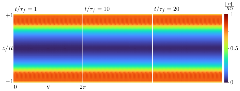
Figure 7: isocontours of the normalized velocity magnitude at $\mbox{Re}_{\Omega}=90$ from $t/\tau_{f}=1$ to 20, where $\tau_{f}=\Omega/2\pi$ is the time it takes to complete a full revolution of the disks. The circumferential cut is taken at the radial distance $r/R=0.8$. At this Reynolds number, the flow is laminar, axisymmetric and planar symmetric about the mid-height plane.

Figure 8: Streamlines of the velocity field in a vertical plane through the axis at $\mbox{Re}_{\Omega}=90$. The flow presents a shear layer formed in between two-toroidal cells similar to what has been reported experimentally in (Ravelet et al., 2008).

We start with the flow at $\mbox{Re}_{\Omega}=90$. Fig. 7 shows instantaneous isocontours of the velocity magnitude from $t\Omega/2\pi=1$ to 20, i.e., over 20 revolutions. The isocontours are visualized in a circumferential cut at the radial distance $r=0.8R$. It is apparent that a steady state is reached in less than one revolution of the impellers. Similarly to the experimental observation in (Ravelet et al., 2008), the flow obtained in these simulations is axisymmetric and planar symmetric about the mid-height plane.

Figure 8 shows streamlines of the velocity field in a plane going through the axis. The figure shows the existence of a flat shear layer at the mid-height plane between two toroidal structures. These vortical structures are the result of the impellers drawing fluid towards their center and expelling it towards the cylinder walls. The fluid recirculates along the cylindrical enclosure’s walls and returns to the center of the device at the mid-height plane thus creating the shear layer. The patterns observed from DNS are in excellent agreement with the structures seen in the photographs of Ravelet et al. (2008) at the same Reynolds number.

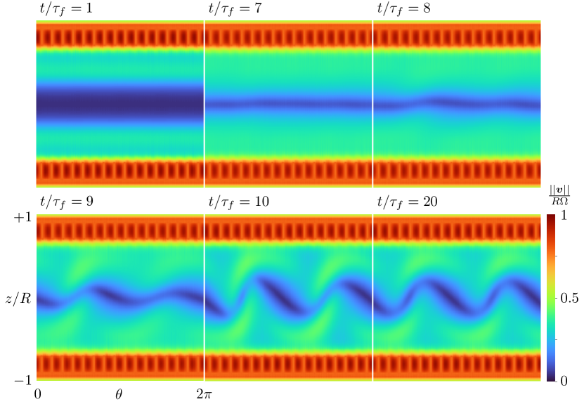
Figure 9: Isocontours of the normalized velocity magnitude at $\mbox{Re}_{\Omega}=360$. The circumferential cut is taken at the radial distance $r/R=0.8$. A sudden transition occurs at $t\Omega/2\pi\sim 8$ leadings to the growth of an azimuthal velocity wave with mode $m=2$.

Isocontours of the normalized velocity magnitude of the flow at $\mbox{Re}_{\Omega}=360$ are shown in Fig. 9. The simulations show that the flow starts with a symmetrical shear layer for $t\Omega/(2\pi)<8$. During this time, the shear layer becomes progressively thinner, which is indicative of increasing shear rate at the mid-height plane. A sudden instability of the shear layer breaks the axisymmetry at $t\Omega/(2\pi)\sim 8$ and leads to the emergence of an azimuthal velocity wave with mode $m=2$. Unlike the lower Reynolds number case, the flow does not reach a steady state until $t\Omega/(2\pi)\sim 14$ when the mode $m=2$ stabilizes.

The physics revealed in our simulations are in accordance with the experimental observations of Ravelet et al. (2008). Long-exposure photographs of tracers in (Ravelet et al., 2008) at $\mbox{Re}_{\Omega}=345$ show the existence of an $m=2$ azimuthal mode. Nore et al. (2003) argue that the $m=2$ mode is due to a Kelvin-Helmholtz instability of the equatorial shear layer. Ravelet et al. (2008) also note that the azimuthal mode in their experiments rotates slowly around the axis. They find that the shear layer completes a full revolution every 300 revolutions of the impellers. However, it is not clear what would cause the rotation of the mode in a preferred direction given that the top and bottom impellers are symmetrical. While we do not observe any noticeable rotation of the shear layer in the 20 rotations simulated here, ruling out the slow dynamics would require significantly longer integration time than we have considered.

4.2 Turbulent regime

4.2.1 Regime identification and torque measurements: Validation against experimental data

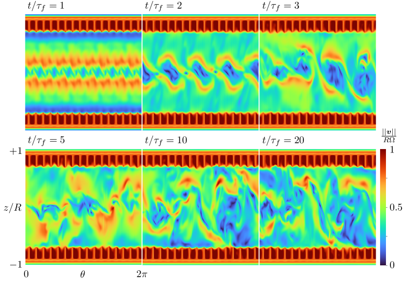
Figure 10: Isocontours of the normalized velocity magnitude at $\mbox{Re}_{\Omega}=2000$. The circumferential cut is taken at the radial distance $r/R=0.8$. An early instability of the shear layer grows rapidly into intense velocity fluctuations. Large vortical structures of size comparable to the disk radius traverse the shear layer.

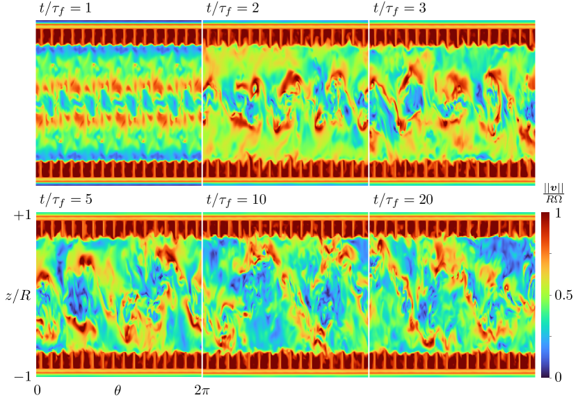
Figure 11: Isocontours of the normalized velocity magnitude at $\mbox{Re}_{\Omega}=4000$. The circumferential cut is taken at the radial distance $r/R=0.8$. The flow is fully turbulent and reaches a statistically stationary state in about 2 revolutions of the impellers.

We now consider the flow at the three higher Reynolds numbers, $\mbox{Re}_{\Omega}=2000$ and 4000. The normalized velocity magnitude at radial location $r=0.8R$ is shown in Fig. 10 and 11. At these higher Reynolds numbers, the symmetries characterizing the low Reynolds number regimes are absent. In these two cases, the transition to turbulence occurs when an azimuthal mode $m=4$ breaks into turbulent fluctuations. The transition takes approximately 5 revolutions of the impellers. Once a statistically stationary state establishes, we observe intense velocity fluctuations sustained in the device with large vortical structures of size comparable to the disk radius traversing the shear layer. The corrugation of isocontours of the velocity magnitude display an increasing distribution of scales with increasing Reynolds number indicating a widening of the inertial range.

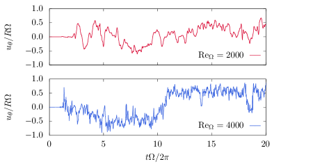
Figure 12: Time series of the normalized azimuthal velocity measured at a reference point located at a radial distance $r=0.9R$ on the mid-plane. The fluctuation rms are 0.30 and 0.51 for the present DNS at $\mbox{Re}_{\Omega}=2000$ and $\mbox{Re}_{\Omega}=4000$, respectively, compared to 0.44 and 0.52 in the experiments of Ravelet et al. (2008).

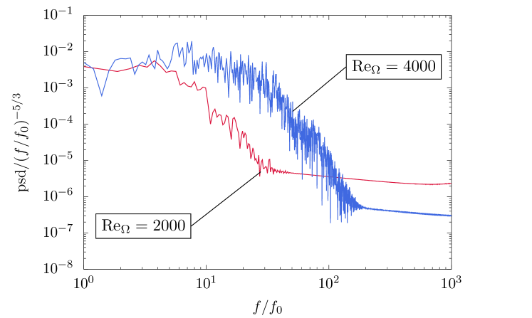
Figure 13: Compensated power spectra. Unlike the case at $\mbox{Re}=4000$, the short bandwidth of the inertial range suggests that turbulence at $\mbox{Re}_{\Omega}=2000$ is not fully developed. Note that $f_{0}=\Omega/(2\pi)$ is the frequency associated with one full revolution of the impellers.

The flow regime can be determined from analysis of the velocity fluctuations at a reference point. Following Ravelet et al. (2008), we measure the azimuthal velocity at a radial location $r=0.9R$ on the mid-height plane. The time series are shown in Fig. 12, where the velocity is normalized by the blade-tip speed $R\Omega$. It is noteworthy that the inertially-driven turbulent von Kármán flow achieves high turbulence intensity. The root mean square (rms) of the azimuthal velocity fluctuations at the sampling location is $u^{\prime}_{\theta}/(R\Omega)=0.30$, 0.51 for $\mbox{Re}_{\Omega}=2000$ and 4000, respectively. In comparison, the experimental fit in (Ravelet et al., 2008) gives $u^{\prime}_{\theta}/(R\Omega)=0.44$ at $\mbox{Re}_{\Omega}=2000$ and $u^{\prime}_{\theta}/(R\Omega)=0.52$ at $\mbox{Re}_{\Omega}=4000$. The lower turbulence intensity at $\mbox{Re}_{\Omega}=2000$ could be due to the shorter averaging period compared to the experiments, where approximately 1000 revolutions are used. The compensated power spectra of the time series are shown in Fig 13. Normalization by the $-5/3$ power-law shows the establishment of the inertial range where the curve is flat. We note that for the $\mbox{Re}_{\Omega}=2000$, the extent of the inertial range is smaller than a decade, which is indicative of transitional turbulence. This observation is in agreement with those of Ravelet et al. (2008) who found that fully developed inertial turbulence is achieved for values of Reynolds number above $\sim 3300$. This regime is achieved in the present DNS at $\mbox{Re}_{\Omega}=4000$ as evidenced by the inertial range extends beyond one decade in Fig. 13.

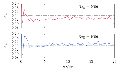
Figure 14: Non-dimensional torque. The mean stationary values are 0.1267 and 0.1472 for $\mbox{Re}_{\Omega}=2000$ and 4000, respectively. These values are in good agreement with the experimentally determined value $K_{p}=0.14$ (Ravelet et al., 2008), represented by the dash-dotted line, in fully developed turbulence.

Another macroscopic observable of interest is the torque exerted by the impellers in order to induce the fluid motion. In laboratory devices, torque is related to the power consumption by the motors driving the impellers. To calculate this quantity, we measure first the total power associated with the force exerted by the immersed boundaries, which is determined from the IB forcing term as

$$\mathcal{P}_{\mathrm{IB}}=\iiint\bm{u}\cdot\bm{F}_{\mathrm{IB}}dV.$$ (13)

Because the impellers rotate at a constant rate $\Omega$, the relationship between power generated by the IB and torque $T$ is

$$T=\frac{\mathcal{P}_{\mathrm{IB}}}{\Omega}.$$ (14)

According to Ravelet et al. (2008), the non-dimensional torque $K_{p}=T/(\rho R^{5}\Omega^{2})$ reaches an asymptotic value $K_{p}\simeq 0.14$, independent of the Reynolds number, for $\mbox{Re}_{\Omega}>3300$. In order to compare with the experiments, we report the temporal evolution of $K_{p}$ in Fig. 14. After a transient of about 4 revolutions of the impellers, the non-dimensional torque reaches a stationary state. The mean $K_{p}$ establishes at 0.1267 and 0.1462 for $\mbox{Re}_{\Omega}=2000$ and 4000, respectively. The values found from these simulations are in excellent agreement with Ravelet et al. (2008) since $K_{p}$ is within a few percent of the experimentally determined asymptotic value.

4.2.2 Characterization of homogeneity and isotropy in fully developed turbulence

(a)

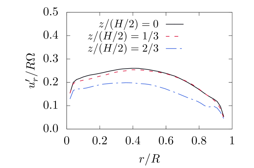
(b)

Figure 15: Radial velocity component. (a) Isocontours of the normalized mean (left half) and rms fluctuations (right half) of the radial velocity at $\mbox{Re}=4000$. (b) Radial profile of the normalized radial velocity fluctuations at three locations along the axis for $\mbox{Re}=4000$.

(a)

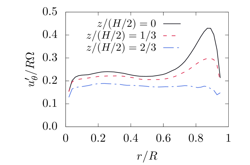
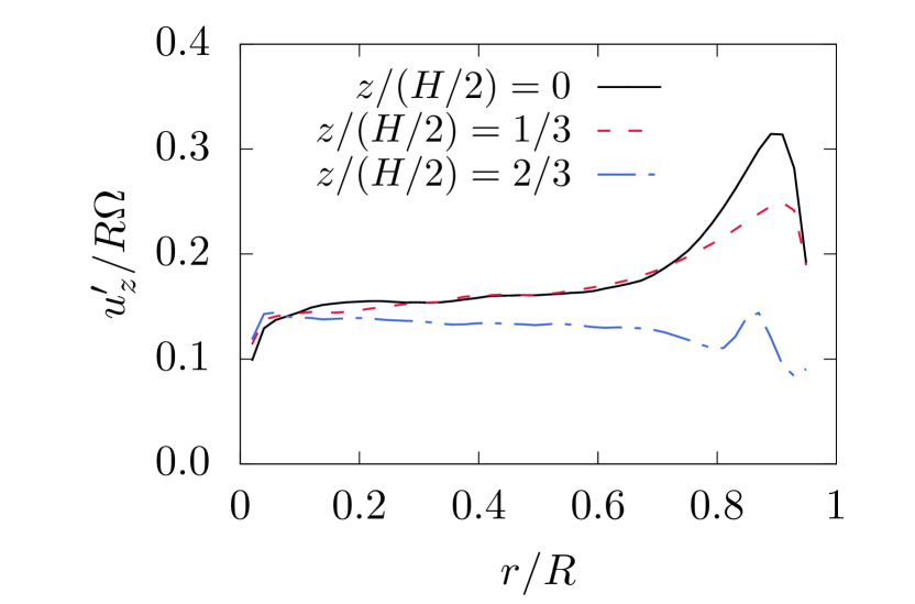
(b)

Figure 16: Azimuthal velocity component. (a) Isocontours of the normalized mean (left half) and rms fluctuations (right half) of the azimuthal velocity at $\mbox{Re}=4000$. (b) Radial profile of the normalized azimuthal velocity fluctuations at three locations along the axis for $\mbox{Re}=4000$.

(a)

(b)

Figure 17: Axial velocity component. (a) Isocontours of the normalized mean (left half) and rms fluctuations (right half) of the axial velocity at $\mbox{Re}=4000$. (b) Radial profile of the normalized axial velocity fluctuations at three locations along the axis for $\mbox{Re}=4000$.

Due to the canonical nature of the turbulent swirling von Kármán flow, it is worthwhile to characterize the nature of the turbulent fluctuations in the fully developed turbulence regime at $\mbox{Re}_{\Omega}=4000$. In particular, we seek to understand whether the turbulent fluctuations in the central region of the flow, i.e., close to the axis and near the mid-height plane are isotropic.

In the present DNS, flow averages and fluctuating quantities are considered once the flow achieves a statistically stationary state, i.e., after 5 revolutions of the disks. Averaging is conducted from the perspective of an observer on a rotating blade using 750 snapshots gathered over 15 rotations. Averages are obtained by grouping data at grid points at equal angles ahead of any one blade (from 0 to 45^∘). Samples at different times are rotated by the corresponding angle.

Figures 15, 16, and 17 show the mean and the rms velocity components normalized by the blade-tip speed $R\Omega$. It is interesting to note that despite the symmetry-breaking instabilities activated at intermediate Reynolds numbers (Lopez et al., 2002; Ravelet et al., 2008; Cortet et al., 2011), the mean flow in the fully developed turbulence regime displays axial and planar symmetries. Much like in the laminar regime at $\mbox{Re}_{\Omega}=90$, the mean flow field consists of two toroidal cells created by fluid ejected radially outward from the blades towards the cylindrical walls, which is then redirected along the walls towards the mid-plane (Fig. 15(a) and 17(a)). Cortet et al. (2010) note that symmetry-breaking transitions may arise in the averaged flow as well, albeit at higher Reynolds numbers than considered here, which raises questions on the stability of the mean flow.

The presence of strong shear in the mid plane due to the two counter-rotating stacked toroidal structures generates large velocity fluctuations, which reach about 30% the tip speed for the azimuthal and radial components. Shear in the boundary layers at the walls of the cylindrical enclosure generates large fluctuations in the axial and azimuthal velocity components also. The central region of $0\leq r/R\leq 0.5$ and $z/(H/2)<1/3$ is of particular interest since it features small mean velocities and little spatial variation in the rms fluctuations.

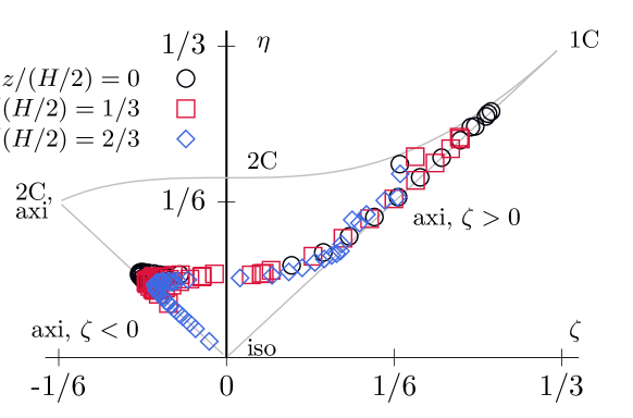
Figure 18: Lumley triangle on the plane of invariants $\zeta-\eta$ of the Reynolds stress anisotropy tensor for $\mbox{Re}=4000$ in three planes normal to the axis. Turbulence in the central region is neither two-component nor truly isotropic.

Turbulence in the central region is not isotropic, since the axial fluctuations are smaller than the other two components, as shown in Fig. 15(b), 16(b), and 17(b). The radial and azimuthal fluctuations decrease in magnitude as we move axially toward the blades. At two thirds of the distance, the rms values of three velocity components are nearly equal and turbulence approaches isotropy.

In order to characterize the anisotropy of the velocity fluctuations, we investigate the Reynolds stress tensor $b_{ij}=\langle u_{i}u_{j}\rangle/\langle u_{k}u_{k}\rangle-\delta_{ij}/3$ and display it in the Lumley triangle (Lumley and Newman, 1977) shown in Fig. 18. Here, $\mathrm{II}_{b}=b_{ij}b_{ji}/2$ and $\mathrm{III_{b}}=(b_{ij}b_{jk}b_{ki})/3$ correspond to the second and third invariants of the tensor $b_{ij}$, while $\zeta=(\mathrm{III_{b}}/2)^{1/3}$ and $\eta=(-\mathrm{II}_{b}/3)^{1/2}$ correspond to the transformed invariants. The data is presented for various radial locations at three axial planes: $z/(H/2)=0,1/3$ and $2/3$. It is apparent that turbulence in the central region (black circles) is neither fully isotropic nor axisymmetric. Moving outwards in the radial direction, the flow transitions to axisymmetric turbulence where the two eigenvalues of the anisotropy tensor are equal and smaller than the third larger eigenvalue. The near wall region displays characteristics of a single component turbulence (labeled ‘1C’ at the top right corner), consistent with the presence of boundary layers near the walls of the enclosure.

5 Conclusions

In this study, we presented results from direct numerical simulations of the swirling von Kármán flow at Reynolds numbers $\mbox{Re}_{\Omega}=90$, 360, 2000 and 4000 in a configuration that reproduces the experiments of Ravelet et al. (2008). While there has been vigorous experimental work on the swirling von Kármán flow, DNS of this flow remain scarce. The numerical simulations presented here display qualitative and quantitative agreement across a range of flow regimes from laminar to fully developed turbulence. This shows that a straightforward implementation of the present IBM on a uniform grid is a powerful tool for the study of such impeller driven flows.

At Reynolds numbers $\mbox{Re}_{\Omega}=90$, the flow consists of two toroidal cells stacked on each other. The flow is axisymmetric and planar symmetric about the mid-plane. The latter symmetry is lost at $\mbox{Re}_{\Omega}=360$ due to the sudden onset of a Kelvin-Helmholtz instability. An azimuthal mode $m=2$ develops on the shear layer at the mid-plane causing the distortion of the tori. These flow patterns conform closely to the dynamics identified in (Ravelet et al., 2008) for the laminar regime, whereby successive symmetry-breaking instabilities appear with increasing Reynolds number. Analysis of time series of velocity fluctuations shows that the case at $\mbox{Re}_{\Omega}=2000$ is transitional, while simulations at $\mbox{Re}_{\Omega}=4000$ achieve fully developed turbulence. The non-dimensional torque computed from DNS matches experimental correlations remarkably well.

Results from the DNS in the fully developed regime show that the mean flow exhibits the same-symmetries as the laminar case $\mbox{Re}_{\Omega}=90$. This suggests that modes created by the low-Reynolds number instabilities are overshadowed by fully developed turbulence. Owing to the strong shear between the two tori, turbulent fluctuations are intense, particularly in the radial and azimuthal directions scaling as 20 to 40% of the blade-tip velocity $R\Omega$. Using the Lumley triangle, we find that the fluctuations in the central region remain anisotropic at $\mbox{Re}_{\Omega}=4000$.

The simulations are enabled by a novel immersed boundary method, which extends the approach of Uhlmann (2005), and is embedded within an incompressible semi-implicit framework with a predictor-corrector step for mass conservation (Desjardins et al., 2008). The approach consists in decoupling the momentum and Eulerian IB forcing equations via operator-splitting. The latter is solved using a backward Euler scheme. Surface integrals are discretized using a triangular mesh of the surface of the immersed body. The forcing terms are computed at the centroids of the triangular faces, which are tracked in a Lagrangian reference frame for moving solids. Our strategy results in an update similar to that of Uhlmann (2005), although derived differently. The robustness and stability of the methodology made the present simulations of the swirling von Kármán flow possible with simple uniform grids.

The use of locally refined grids as in (Kang et al., 2009) could improve the solutions near the immersed boundaries. However, for moving boundaries, such as impellers, it is not clear yet how this refinement can be achieved without incurring the same penalties found in methods using body-conformal meshes. Coupling the present IBM with overset grids could provide a way forward, and shall be investigated in future studies.

Appendix A Effect of grid resolution on the measured torque

To demonstrate the grid convergence of our computational method in the swirling von Kármán flow cases, we present the results from two auxiliary simulations at $\mbox{Re}_{\Omega}=4000$. Compared to the reference simulation in Tab. 4, these two additional simulations are performed on a coarser and a finer grid. The former is a uniform Cartesian grid with $256\times 342\times 256$ points, yielding a constant resolution $R/\Delta x=128$. The fine grid has $640\times 896\times 640$ points corresponding to a resolution of $R/\Delta x=320$. Note that the simulation in Tab. 4 has a size $512\times 688\times 512$ and resolution $R/\Delta x=256$.

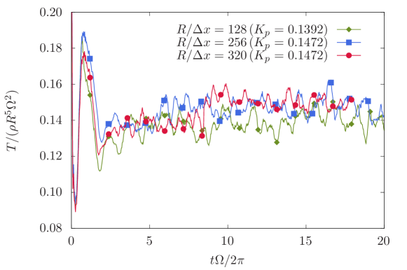
Figure 19: Evolution of the non-dimensional torque at the three mesh resolutions $R/\Delta x=$128, 256, and 320. The average non-dimensional torque, $K_{p}$, converges to 0.1472.

Figure 19 shows the evolution of the non-dimensional torque from three three runs. The average non-dimensional torque, $K_{p}$, computed from the fifth revolution and onward, converges to 0.1472 for $R/\Delta x=256$ and 320. This convergence study shows that the fluid stresses on the impellers are well captured by resolutions $R/\delta x=256$ and beyond for swirling von Kármán flow at $\mbox{Re}_{\Omega}=4000$.

References

- Akselvoll [1995] Knut Akselvoll. Large Eddy Simulation of Turbulent Confined Coannular Jets and Turbulent Flow over a Backward Facing Step /. PhD thesis, Stanford University, Stanford, CA, 1995.
- Balaras [2004] Elias Balaras. Modeling complex boundaries using an external force field on fixed Cartesian grids in large-eddy simulations. Computers & Fluids, 33(3):375–404, March 2004. ISSN 0045-7930. doi: 10.1016/S0045-7930(03)00058-6.
- Batchelor [1951] G. K. Batchelor. Note on a class of solutions of the Navier-Stokes equations representing steady rotationally-symmetric flow. The Quarterly Journal of Mechanics and Applied Mathematics, 4(1):29–41, January 1951. ISSN 0033-5614. doi: 10.1093/qjmam/4.1.29.
- Bertrand et al. [1980] J. Bertrand, J. P. Couderc, and H. Angelino. Power consumption, pumping capacity and turbulence intensity in baffled stirred tanks: Comparison between several turbines. Chemical Engineering Science, 35(10):2157–2163, January 1980. ISSN 0009-2509. doi: 10.1016/0009-2509(80)85040-8.
- Burnishev and Steinberg [2014] Yuri Burnishev and Victor Steinberg. Torque and pressure fluctuations in turbulent von Karman swirling flow between two counter-rotating disks. I. Physics of Fluids, 26(5):055102, May 2014. ISSN 1070-6631. doi: 10.1063/1.4873201.
- Choi and Moin [1994] Haecheon Choi and Parviz Moin. Effects of the Computational Time Step on Numerical Solutions of Turbulent Flow. Journal of Computational Physics, 113(1):1–4, July 1994. ISSN 0021-9991. doi: 10.1006/jcph.1994.1112.
- Cortet et al. [2010] P.-P. Cortet, A. Chiffaudel, F. Daviaud, and B. Dubrulle. Experimental Evidence of a Phase Transition in a Closed Turbulent Flow. Physical Review Letters, 105(21), November 2010. ISSN 0031-9007, 1079-7114. doi: 10.1103/PhysRevLett.105.214501.
- Cortet et al. [2011] P-P Cortet, E Herbert, A Chiffaudel, F Daviaud, B Dubrulle, and V Padilla. Susceptibility divergence, phase transition and multistability of a highly turbulent closed flow. Journal of Statistical Mechanics: Theory and Experiment, 2011(07):P07012, July 2011. ISSN 1742-5468. doi: 10.1088/1742-5468/2011/07/P07012.
- Debue et al. [2018] P. Debue, V. Shukla, D. Kuzzay, D. Faranda, E.-W. Saw, F. Daviaud, and B. Dubrulle. Dissipation, intermittency, and singularities in incompressible turbulent flows. Physical Review E, 97(5), May 2018. ISSN 2470-0045, 2470-0053. doi: 10.1103/PhysRevE.97.053101.
- Desjardins et al. [2008] O. Desjardins, G. Blanquart, G. Balarac, and H. Pitsch. High order conservative finite difference scheme for variable density low Mach number turbulent flows. Journal of Computational Physics, 227(15):7125–7159, July 2008. ISSN 0021-9991. doi: 10.1016/j.jcp.2008.03.027.
- Dubrulle [2019] Bérengère Dubrulle. Beyond Kolmogorov cascades. Journal of Fluid Mechanics, 867, May 2019. ISSN 0022-1120, 1469-7645. doi: 10.1017/jfm.2019.98.
- Fadlun et al. [2000] E. A. Fadlun, R. Verzicco, P. Orlandi, and J. Mohd-Yusof. Combined Immersed-Boundary Finite-Difference Methods for Three-Dimensional Complex Flow Simulations. Journal of Computational Physics, 161(1):35–60, June 2000. ISSN 0021-9991. doi: 10.1006/jcph.2000.6484.
- Kang et al. [2009] Seongwon Kang, Gianluca Iaccarino, and Frank Ham. DNS of buoyancy-dominated turbulent flows on a bluff body using the immersed boundary method. Journal of Computational Physics, 228(9):3189–3208, May 2009. ISSN 0021-9991. doi: 10.1016/j.jcp.2008.12.037.
- Kármán [1921] Th V. Kármán. über laminare und turbulente Reibung. ZAMM - Journal of Applied Mathematics and Mechanics / Zeitschrift für Angewandte Mathematik und Mechanik, 1(4):233–252, 1921. ISSN 1521-4001. doi: 10.1002/zamm.19210010401.
- Kim and Choi [2006] Dokyun Kim and Haecheon Choi. Immersed boundary method for flow around an arbitrarily moving body. Journal of Computational Physics, 212(2):662–680, March 2006. ISSN 0021-9991. doi: 10.1016/j.jcp.2005.07.010.
- Kim et al. [2001] Jungwoo Kim, Dongoo Kim, and Haecheon Choi. An Immersed-Boundary Finite-Volume Method for Simulations of Flow in Complex Geometries. Journal of Computational Physics, 171(1):132–150, July 2001. ISSN 0021-9991. doi: 10.1006/jcph.2001.6778.
- Kreuzahler et al. [2014] S. Kreuzahler, D. Schulz, H. Homann, Y. Ponty, and R. Grauer. Numerical study of impeller-driven von Kármán flows via a volume penalization method. New Journal of Physics, 16(10):103001, October 2014. ISSN 1367-2630. doi: 10.1088/1367-2630/16/10/103001.
- Kuzzay et al. [2015] Denis Kuzzay, Davide Faranda, and Bérengère Dubrulle. Global vs local energy dissipation: The energy cycle of the turbulent von Kármán flow. Physics of Fluids, 27(7):075105, July 2015. ISSN 1070-6631. doi: 10.1063/1.4923750.
- Lai and Peskin [2000] Ming-Chih Lai and Charles S. Peskin. An Immersed Boundary Method with Formal Second-Order Accuracy and Reduced Numerical Viscosity. Journal of Computational Physics, 160(2):705–719, May 2000. ISSN 00219991. doi: 10.1006/jcph.2000.6483.
- Liu et al. [1998] C. Liu, X. Zheng, and C. H. Sung. Preconditioned Multigrid Methods for Unsteady Incompressible Flows. Journal of Computational Physics, 139(1):35–57, January 1998. ISSN 0021-9991. doi: 10.1006/jcph.1997.5859.
- Lopez et al. [2002] J. M. Lopez, J. E. Hart, F. Marques, S. Kittelman, and J. Shen. Instability and mode interactions in a differentially driven rotating cylinder. Journal of Fluid Mechanics, 462:383–409, July 2002. ISSN 1469-7645, 0022-1120. doi: 10.1017/S0022112002008649.
- Lu and Dalton [1996] X. Y. Lu and C. Dalton. Calculation of the timing of vortex formation from an oscillating cylinder. Journal of Fluids and Structures, 10(5):527–541, July 1996. ISSN 0889-9746. doi: 10.1006/jfls.1996.0035.
- Lumley and Newman [1977] John L. Lumley and Gary R. Newman. The return to isotropy of homogeneous turbulence. Journal of Fluid Mechanics, 82(1):161–178, August 1977. ISSN 1469-7645, 0022-1120. doi: 10.1017/S0022112077000585.
- Maurer et al. [1994] J. Maurer, P. Tabeling, and G. Zocchi. Statistics of Turbulence between Two Counterrotating Disks in Low-Temperature Helium Gas. EPL (Europhysics Letters), 26(1):31, 1994. ISSN 0295-5075. doi: 10.1209/0295-5075/26/1/006.
- Mittal and Iaccarino [2005] Rajat Mittal and Gianluca Iaccarino. Immersed Boundary Methods. Annual Review of Fluid Mechanics, 37(1):239–261, 2005. doi: 10.1146/annurev.fluid.37.061903.175743.
- Monchaux et al. [2008] Romain Monchaux, Pierre-Philippe Cortet, Pierre-Henri Chavanis, Arnaud Chiffaudel, François Daviaud, Pantxo Diribarne, and Bérengère Dubrulle. Fluctuation-Dissipation Relations and Statistical Temperatures in a Turbulent von Kármán Flow. Physical Review Letters, 101(17), October 2008. ISSN 0031-9007, 1079-7114. doi: 10.1103/PhysRevLett.101.174502.
- Nicolaou et al. [2015] L. Nicolaou, S. Y. Jung, and T. A. Zaki. A robust direct-forcing immersed boundary method with enhanced stability for moving body problems in curvilinear coordinates. Computers & Fluids, 119:101–114, September 2015. ISSN 0045-7930. doi: 10.1016/j.compfluid.2015.06.030.
- Nore et al. [2003] C. Nore, L. S. Tuckerman, O. Daube, and S. Xin. The 1[ratio]2 mode interaction in exactly counter-rotating von Kármán swirling flow. Journal of Fluid Mechanics, 477, February 2003. ISSN 0022-1120, 1469-7645. doi: 10.1017/S0022112002003075.
- Nore et al. [2004] C. Nore, M. Tartar, O. Daube, and L. S. Tuckerman. Survey of instability thresholds of flow between exactly counter-rotating disks. Journal of Fluid Mechanics, 511:45–65, July 2004. ISSN 1469-7645, 0022-1120. doi: 10.1017/S0022112004008559.
- Nore et al. [2018] C. Nore, D. Castanon Quiroz, L. Cappanera, and J.-L. Guermond. Numerical simulation of the von Kármán sodium dynamo experiment. Journal of Fluid Mechanics, 854:164–195, November 2018. ISSN 0022-1120, 1469-7645. doi: 10.1017/jfm.2018.582.
- Odier et al. [1998] P. Odier, J.-F. Pinton, and S. Fauve. Advection of a magnetic field by a turbulent swirling flow. Physical Review E, 58(6):7397–7401, December 1998. ISSN 1063-651X, 1095-3787. doi: 10.1103/PhysRevE.58.7397.
- Peskin [1972] Charles S Peskin. Flow patterns around heart valves: A numerical method. Journal of Computational Physics, 10(2):252–271, October 1972. ISSN 0021-9991. doi: 10.1016/0021-9991(72)90065-4.
- Peskin [2002] Charles S. Peskin. The immersed boundary method. Acta Numerica, 11:479–517, January 2002. ISSN 1474-0508, 0962-4929. doi: 10.1017/S0962492902000077.
- Pierce [2001] C. D. Pierce. Progress-Variable Approach for Large-Eddy Simulation of Turbulent Combustion. PhD thesis, Stanford University, Stanford, CA, 2001.
- Pierce and Moin [2004] Charles D. Pierce and Parviz Moin. Progress-variable approach for large-eddy simulation of non-premixed turbulent combustion. Journal of Fluid Mechanics, 504:73–97, April 2004. ISSN 1469-7645, 0022-1120. doi: 10.1017/S0022112004008213.
- Ravelet et al. [2005] F. Ravelet, A. Chiffaudel, F. Daviaud, and J. Léorat. Toward an experimental von Kármán dynamo: Numerical studies for an optimized design. Physics of Fluids, 17(11):117104, November 2005. ISSN 1070-6631. doi: 10.1063/1.2130745.
- Ravelet [2005] Florent Ravelet. Bifurcations globales hydrodynamiques et magnetohydrodynamiques dans un ecoulement de von Karman turbulent. PhD thesis, Ecole Polytechnique X, September 2005.
- Ravelet et al. [2008] Florent Ravelet, Arnaud Chiffaudel, and François Daviaud. Supercritical transition to turbulence in an inertially driven von Kármán closed flow. Journal of Fluid Mechanics, 601:339–364, April 2008. ISSN 1469-7645, 0022-1120. doi: 10.1017/S0022112008000712.
- Roma et al. [1999] Alexandre M Roma, Charles S Peskin, and Marsha J Berger. An Adaptive Version of the Immersed Boundary Method. Journal of Computational Physics, 153(2):509–534, August 1999. ISSN 0021-9991. doi: 10.1006/jcph.1999.6293.
- Schäfer et al. [1996] M. Schäfer, S. Turek, F. Durst, E. Krause, and R. Rannacher. Benchmark Computations of Laminar Flow Around a Cylinder. In Ernst Heinrich Hirschel, editor, Flow Simulation with High-Performance Computers II: DFG Priority Research Programme Results 1993–1995, Notes on Numerical Fluid Mechanics (NNFM), pages 547–566. Vieweg+Teubner Verlag, Wiesbaden, 1996. ISBN 978-3-322-89849-4. doi: 10.1007/978-3-322-89849-4_39.
- Uhlmann [2005] Markus Uhlmann. An immersed boundary method with direct forcing for the simulation of particulate flows. Journal of Computational Physics, 209(2):448–476, November 2005. ISSN 0021-9991. doi: 10.1016/j.jcp.2005.03.017.
- Vanella and Balaras [2009] Marcos Vanella and Elias Balaras. A moving-least-squares reconstruction for embedded-boundary formulations. Journal of Computational Physics, 228(18):6617–6628, October 2009. ISSN 0021-9991. doi: 10.1016/j.jcp.2009.06.003.
- Williamson [1989] C. H. K. Williamson. Oblique and parallel modes of vortex shedding in the wake of a circular cylinder at low Reynolds numbers. Journal of Fluid Mechanics, 206:579–627, September 1989. ISSN 0022-1120, 1469-7645. doi: 10.1017/S0022112089002429.
- Yang and Balaras [2006] Jianming Yang and Elias Balaras. An embedded-boundary formulation for large-eddy simulation of turbulent flows interacting with moving boundaries. Journal of Computational Physics, 215(1):12–40, June 2006. ISSN 0021-9991. doi: 10.1016/j.jcp.2005.10.035.
- Zandbergen and Dijkstra [1987] P J Zandbergen and D Dijkstra. Von Karman Swirling Flows. Annual Review of Fluid Mechanics, 19(1):465–491, 1987. doi: 10.1146/annurev.fl.19.010187.002341.