Estimating expectation values using approximate quantum states
Abstract
We introduce an approximate description of an –qubit state, which contains sufficient information to estimate the expectation value of any observable to a precision that is upper bounded by the ratio of a suitably–defined seminorm of the observable to the square root of the number of the system’s identical preparations , with no explicit dependence on . We describe an operational procedure for constructing the approximate description of the state that requires, besides the quantum state preparation, only single–qubit rotations followed by single–qubit measurements. We show that following this procedure, the cardinality of the resulting description of the state grows as . We test the proposed method on Rigetti’s quantum processor unit with 12, 16 and 25 qubits for random states and random observables, and find an excellent agreement with the theory, despite experimental errors.
1 Introduction
Quantum density operators represent our knowledge of the state of quantum systems and give us a way to calculate expectation values and predict experimental results via the Born rule. Our knowledge of a system’s density operator is equivalent to our ability to calculate the expectation value of any observable of the system. However, for an –body system, reconstructing the system’s density operator requires the knowledge of exponentially many numbers in . This in turn translates into practical difficulties in estimating and storing density operators, in the form of density matrices, even for systems composed of just a few tens of qubits.
Over the last few years, there has been a surge of interest in devising protocols to reduce the resources required to estimate and classically store quantum states [1, 2, 3, 4, 5, 6, 7, 8, 9]. There have been numerous approaches to reduce the cost of performing quantum state tomography by assuming that the state of the system has a specific structure. These approaches include, for example: matrix product states tomography [3], where the state is assumed to have an efficient matrix product state representation as a matrix; neural network tomography [6, 7], where the state is assumed to have an efficient deep neural network representation; and compressed sensing tomography [4, 5], where the state is assumed to have a low-rank density matrix representation. The theory of Probably Approximately Correct (PAC) learning was utilised in [2] to show that if, instead of full tomography, we are interested in approximating with high probability the expectation values of observables drawn from a distribution, then only polynomially–many samples in of the observables’ expectation values are required. It was later also shown [8] that estimating with high probability the expectation values of a set of observables can be achieved using only polynomially–many copies in of the system. As for storage, it is well established [1] that quantum states that can be represented as low bond–dimension matrix product states can be efficiently stored on classical computers. Recently it was shown [9] that a general quantum state of qubits can be approximately described using its inner product with an order of stabiliser states. This result thus provides a polynomial improvement for classically storing quantum states over a brute–force approach of storing density matrices. In Sec. 4 we discuss these and other works in connection to the results presented in this paper.
The growth of the number of copies of the system in for estimation and the considerable requirements in for classically storing the information associated with a generic quantum state lead to the question of whether a protocol that significantly reduces or eliminates the dependence on is admissible. In this work, we give an affirmative answer to the question. Instead of focusing on the estimation and storage of the density matrix, we start by considering the equivalent problem of calculating the expectation value of any observable of the system up to a certain precision. In this article we show that, for a system of qubits, the expectation value of any observable can be calculated with arbitrary precision with a number of copies of the system independent of , but dependent on a properly–defined seminorm of the observable. The information obtained through the measurements on the copies of the system will be used to form an approximate description of the quantum state – a description with a cardinality that grows linearly in and thus can be constructed and stored for large systems. The method for estimating expectation values, and the exact definition of an observable seminorm and of the storage approximate quantum state will be given in the next section.
2 Expectation value estimation and the approximate quantum state
We will consider specifically a system of qubits. However, the considerations that will be made are applicable in general to other systems, with finite and infinite–dimensional Hilbert spaces, since they are based on the general theory of irreducible representations of groups which provide explicit forms for a basis in the space of linear bounded operators defined on a Hilbert space. We refer the reader to Refs. [10, 11] where these considerations have been developed.
We start by presenting the method to estimate the expectation value of any observable and notion of the approximate state for a single–qubit system. We then generalise these ideas for the more general –qubit case.
2.1 One qubit
A single–qubit density operator can be written as [10, 11]
| (1) |
with the unitary spherical surface as integration domain, , with , is a unit vector in , is the probability of obtaining the result when measuring the qubit in the eigenbasis of , where is a vector of the Pauli operators, and is the 1–qubit kernel operator given by
| (2) |
see App. A for more details.
Let us define a single–qubit (unbiased) estimator function
| (3) |
where the represents the argument of the function , i.e. a single–qubit observable (for a lighter notation we sometime omit the explicit dependence of the estimator on ). In particular, the expectation value of the Pauli operator , with and and , can be written in terms of as
| (4) |
Calculating the estimator of the Pauli operators we arrive at
| (5) | ||||
| (6) |
The estimator is a random variable due to its dependence on the stochastic measurement outcome and the random unit vector . Hereafter, unless noted otherwise, we use the subscript to index and subscript to index . In App. A we show that the variance of the estimator is upper bounded by ,
| (7) |
Since is independent of and , it is deterministic and thus has a null variance.
Equation (4) implies that we can construct an estimate of using the following Monte Carlo sampling procedure:
-
1.
Sample a point uniformly from the surface of a unit sphere,
-
2.
prepare the qubit in the state and measure it in the eigenbasis of ,
-
3.
record the outcome ,
-
4.
repeat steps 1–3 times.
The estimate of , which we denote by , is simply given by the average of corresponding estimator over the data set:
| (8) |
where is the unit vector sampled at the th iteration and is the corresponding measurement outcome. Note that the estimate for any value of and it has zero variance. Moreover, by construction, in the limit , , for . The value of determines the precision of the estimation. For sufficiently large, has a normal statistical error, which due to Eq. (7) is smaller than or equal to .
The measurement in the eigenbasis of , at step 2 above, can be implemented by first applying a unitary operator , that rotates this basis to the eigenbasis of , and then measuring in the eigenbasis (the computational basis). This unitary operator is given by , where . We call the vector the -th snapshot of the qubit system. We refer to the collection of the snapshots, , that we obtain following the sampling procedure above, as the approximate quantum state, as it enables us to estimate the expectation value of any single–qubit observable to a certain precision as we now describe.
Let be a single–qubit observable, expanded in the Pauli basis ,
| (9) |
Given the estimated expectation values of , by linearity of the estimator function (3), we can construct an estimate of as
| (10) |
We prove in App. A that for sufficiently large, has a normal statistical error smaller than or equal to , that is
| (11) |
where Std stands for ‘standard deviation’ and
| (12) |
is a seminorm of that depends on its expansion in the Pauli operator basis.
2.2 qubits
The method developed for one qubit in the previous subsection is easily generalised to qubits, in the assumptions that the qubits are distinguishable and that a qubit–specific measurement capability is available. The space of the –qubit system is the tensor product of the single–qubit spaces and thus we can write a general –qubit density operator as [10, 11]
| (13) |
where is a shorthand for , the –qubit kernel operator equals to the tensor product of single–qubit kernels
| (14) |
and represents the joint probability of finding the outcome when measuring the qubits in the product eigenbasis of . Similarly to the single qubit case, this measurement can be implemented with single–qubit rotations followed by a measurement in the computational basis on each qubit.
We define the –qubit (unbiased) estimator function
| (15) |
As a result of the tensor product structure of the kernel operator, , where , , is a monomial of Pauli operators (a ‘Pauli monomial’ or a ‘Pauli string’ for short), and hereafter , is simply the product of the corresponding single–qubit random variables,
| (16) |
Similarly to the single qubit case of the previous section, we can write the expectation value of with respect to the state of the system in terms of as
| (17) | ||||
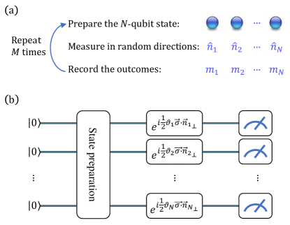
Eq. (17) implies that an estimate of can be calculated by performing the single–qubit tomographic procedure introduced in the above section, in parallel on all of the qubits, as in Fig. 1. We call the vector the th snapshot of a system of qubits, and we refer to a set of such independent snapshots as the approximate state of the –qubit system.
The use of single–qubit Haar–random basis measurements was recently proposed, and experimentally implemented, to probe certain properties of an –qubit system, such as purity [12, 13] and the Frobenius inner product of two states [14]. In light of these results, as we now show, the measurement protocol we introduced above is a universal protocol for estimating the expectation value of any –qubit observable. The protocol is efficient in terms of time and space resources, as long as the observable admits an efficient representation in the Pauli basis and has a small seminorm (e.g. not growing exponentially with ).
To start with, we can use the approximate state to calculate an estimate of as
| (18) |
where the first equality follows from Eq. (16). We show in App. B that for sufficiently large, () has a normal statistical error that is smaller than or equal to , where represents the weight of , i.e., the number of qubits on which it acts non–trivially. Note that the estimated expectation value for the –qubit identity operator and it has zero variance.
With the ability to efficiently calculate the estimated expectation value of any given Pauli monomial operator, we can estimate the expectation value of –qubit observables. Let be an –qubit observable such that
| (19) |
From linearity of the estimator function (15) and from Eq. (18), the estimated expectation value of is given by
| (20) |
Similar to , is an unbiased estimate, i.e., in the limit . Practically, for the efficient calculation of (20), the sum on should have at most a polynomial number of terms in .
While we assumed in Eq. (19) that the observable admits an efficient representation in terms of Pauli monomials, as a result of the tensor product structure of the kernel operator, Eq. (14), our procedure is efficient to calculate the expectation value of any operator of the form
| (21) |
where is a single-qubit operator (on the th qubit space). If this is the case then,
| (22) |
Note that any Pauli monomial is a special case of .
We show in App. B that the standard deviation of has the upper bound
| (23) |
with the seminorm of defined as
| (24) |
where the sum is extended to all values of and except , is the number of indices for which , if there exists a such that and otherwise. Eq. (24) reduces to Eq. (12) when is an observable on a single–qubit space.
Importantly, in this procedure, the expectation values estimation error has no global dependence on the system size . The error only depends on the observable seminorm and the number of snapshots. One could argue that the presence in the seminorm of reflects an exponential growth of the estimates’ variance in , as, for example, for an observable given by the tensor product of Pauli operators, which has seminorm . However, the seminorm is a property of the observable and not of the dimension of the space: an –qubit observable and its extension to a larger –qubit space, , have the same seminorm (24), independent of . Irrespective of , because of Eq. (23), the expectation values of all observables with unit seminorm can be obtained with statistical error bounded by . Any observable with seminorm different from zero can be obtained from an observable with unit seminorm through multiplication by a real number, representing in fact the observable’s seminorm. For a given number of identical preparations and measurements, the statistical error in the expectation value of the generic observable has a bound only dependent on how “large” the observable is. In App. B, we also explain how the seminorm , defined by
| (25) |
divided by , with representing the weight of , is generally a good approximation for the standard deviation of . This result may be important for applications of the method since can be significantly smaller than and since, for a chosen statistical error, the number of identical preparations required is inversely proportional to the variance of . See App. C for further details.
We close this part with a remark on the notion of the approximate quantum state, . We have shown that the approximate description of the state, as we have defined it, comes with an explicit operational procedure to estimate the expectation value of any generic observable with a rigorous bound on the estimation statistical error. Therefore, the approximate state together with the rule (20) provides a description of a physical system in terms of statistical inferences based on observed experimental data and, in principle, could be assumed as primitive concepts instead, or, at least, as not requiring the existence of density operators and the Born rule.
3 Experimental results
As a proof–of–concept, we have tested the theory on Rigetti Computing quantum processor unit (QPU), Aspen7-28Q-A, with three systems, involving and qubits, respectively. In each experiment the system is prepared in a random state. The state preparation circuit is composed of two layers of gates applied to the computational state . In the first layer, the gates are chosen at random from a flat distribution over the single–qubit gate set and applied to qubits, chosen at random. While in the second layer the two–qubit gate is applied to of pairs of qubits, chosen at random, with different values of sampled uniformly from . This gate composition results in shallow quantum circuits with random single–qubit gates and random two–qubit gates, to ensure that the experimentally prepared state has a high fidelity with the target state.
For each system, an approximate description of the prepared state was obtained using snapshots (to check the results to accuracy). The approximate state was then used to estimate the expectation value of two sets of observables: (1) 20 random observables, (2) 20 random projectors onto computational basis states (we have selected 20 for the number of states so that it would be visually ‘easy’ to check the results in Fig. 2 against the second standard deviation given it is at 95%). Each random observable in the first set is a linear combination of 20 Pauli monomials. Each Pauli monomial is constructed by randomly sampling from the set for each qubit, whereas the linear combination coefficients (the ’s) are sampled uniformly from the . The projectors onto computational basis states were sampled uniformly from the set . For simplicity in the analysis, the 20 random observables are normalised to have a unit seminorm (the projectors already have unit seminorm with probability exponentially close to 1 as a function of , see App. C).
Fig. 2 shows the results for the 25–qubit experiment. In this figure, we compare the estimated expectation values of random observables and of random computational basis projectors to their expectation values with respect to the 25–qubit target state. The results are plotted as a function of the number of snapshots. Table 1 summarises the experimental results of the –, – and –qubit systems for snapshots. The figure and the table show that the experimental results generally mirror the theory, with the fraction of estimates within one and two standard deviations from their true values not far from and respectively. Other than statistical considerations, the cases with a fraction of the estimates greater than the expected percentages from a normal distribution can be explained in terms of how tightly the observables’ seminorms bound the standard deviation of the estimators, in particular for the case of the projectors.
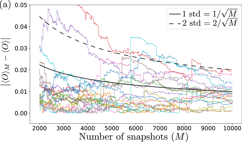
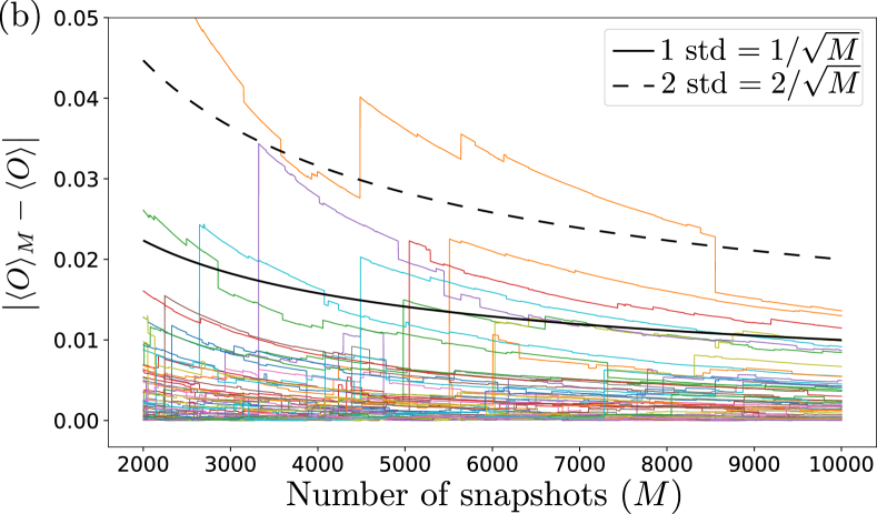
To complete the picture, including an explanation for the cases of a lower fraction of the estimates than predicted, we need to start examining the effects of hardware errors. It is worth noting that we obtain agreement with the theory despite an order of (averaged) readout error per qubit, which amounts to flipping the measurement outcome from to and vice versa. The resilience of our protocol to single–qubit readout errors can be attributed to the randomness of the measurement bases, as was discussed in [15]. Moreover, the following considerations provide additional insights in the robustness of the estimation protocol to readout errors.
Firstly, let us consider the estimation of the expectation value of single–qubit observable. Let be the approximate state description composed of snapshots. Suppose that in of the snapshots we obtained the erroneous measurement outcome, . The estimation of the expectation value of any single–qubit Pauli operator () is
| (26) |
where is the erroneous outcome. Since we arrive at
| (27) |
which, for sufficiently large and , can be approximated by
| (28) |
Therefore, for a single–qubit observable we arrive at
| (29) |
Thus, the readout error introduces an attenuator to each coefficient different than in the expectation value.
Moving to the –qubit case, we first note that only odd numbers of readout errors per snapshot contribute to the estimation error of an –qubit expectation value. This is because the estimated expectation value is calculated via a product of the measurement outcomes which take values , c.f. Eq. (18). Therefore, if a given snapshot includes readout errors on an even number of qubits, there are even number of erroneous outcomes such that , and the estimated expectation value remains unaffected by these errors. Let be the probability that in a given snapshot there is an odd number of readout errors on qubits. Given a readout error per qubit,
| (30) |
Similarly to the single qubit analysis, one can then show that the expectation value of a Pauli monomial with weight is
| (31) |
We therefore obtain that the estimated expectation value of an –qubit observable is given by
| (32) |
This equation indicates that the readout error does not depend on . It introduces an attenuator to each term in the expectation value. Since the attenuator is an exponentially decreasing function in the weight , only low–weight Pauli monomials contribute to the expectation value . Thus, the proposed method is robust against readout error when estimating expectation values that have contributions dominantly from low–weight Pauli monomials (this does not necessarily exclude observables, such as projectors, that have contributions from all Pauli monomials: the contribution of higher weight Pauli monomials could be small on a class of states of interest, as in the case of the low entanglement states of this section’s random projectors experiment). Finally, we remark that other errors, e.g. gate operation errors, could be included in this framework in a similar fashion and that, clearly, (32) is easily generalisable to the case of different readout errors per qubit.
4 Related work
Quantum state tomography. In general, estimating an –qubit state to error in trace distance requires copies of the state [16, 17]. The estimation of the density matrix with our tomographic procedure does not break this lower bound. If we choose the basis of –qubit Pauli operators, Eq. (23) tells us that a few matrix elements will require to be exponentially large in . A different basis, such as the standard basis , has exponentially many matrix elements bounded by 1. However, calculating the trace distance requires adding exponentially many of them, creating again the need for an exponentially large . The key point of this paper, however, is to be able to estimate approximately and efficiently expectation values without resorting to the notion of density matrix.
Shadow tomography. In shadow tomography the task is to estimate with high probability the expectation values of a set of observables, to a certain precision . It was shown that [8, 18] this can be done using copies of the state, by implementing a non–local measurement on all copies of the state. Recently, these results were improved [19]. The authors of [19] proposed an algorithm where copies of the state, with , allow one to predict the expectation values of observables, , to a precision . The norm depends on the particular measurement procedure used in the algorithm. For example, for random Pauli measurements the authors show (Proposition 3 there) that for a -local observable , where denotes the spectral norm.
The algorithm of [19] has a similar structure to the algorithm proposed in this work. Similarly to [19], the choice of randomised single–qubit measurement directions of Eq. (13) is not the only possible one. The framework of [10, 11] generates valid formulas for any irreducible projective representation in the space of the system, including for example the Clifford group and the representation of in the space of a spin . Furthermore, one could also easily derive a general expression for the norm, bound of the standard deviation of the estimator, as multiplied by a factor only dependent on the group representation chosen. It is important to note, however, that the use of the Cauchy-Schwarz inequality in the derivation would generate suboptimal norms, often exponentially larger than the true standard deviation of the estimator. A tight norm (or seminorm) is key, as it gives a guarantee of performance with a lower number of preparations, especially if the separation from a suboptimal one is exponential. The closeness to the standard deviation of the estimator is what justifies the importance of of (25): can be exponentially smaller than norms depending exponentially on the locality or on the dimension of the system (App. C for the case of projectors onto the computational basis).
Finally, while the task in shadow tomography is to estimate with high probability the expectation values of a set of observables, to a certain precision , we focus here on the estimation with high probability the expectation values of a given, yet arbitrary, observable to a certain precision . We show that accomplishing this task requires copies of the state. If a certain precision is required for the combined evaluation of expectation values of several observables, one would simply calculate the joint probability of several normal variables of being smaller than a certain value which would lead to a log contribution to the error in the number of observables.
5 Conclusions and outlook
We have introduced a concept of approximate description of a quantum state for a system of qubits. We have shown that the approximate state comes with an explicit operational procedure to estimate the expectation value of any observable that admits an efficient representation in the Pauli basis with statistical error only dependent on the cardinality of the approximate quantum state and on the observable’s seminorm, independent of and growing at most exponentially with the locality of the observable. The operational procedure to obtain the approximate state, other than the initial state preparations, only requires single–qubit operations and measurement. The natural robustness of random single–qubit operations to experimental noise, as we saw in the experimental results and also discussed in [15], suggests that the proposed protocol could be appropriate for NISQ computers.
We expect the notion of the approximate quantum state to enable improvement over existing variational optimisation methods, as it would not require separate iterations for each set of values of the parameters. Machine learning optimisations, in particular for generative models known as Born Machines [20], may be an interesting case, since the explicit dependence of the expectation values of the projectors onto computational basis states on the variational parameters [21] may be obtained even for a large number of qubits, since, as shown in App. B, the estimators for the projectors onto computational basis state have, with high probability, variance bounded by 1 for all values of .
The definition of the snapshots, constituting an approximate quantum state, can be generalised, too. The snapshots can in fact be derived from a group different from . This generalisation has interest that goes beyond the purely mathematical exercise. As we have seen, tomography works well for observables expressed as linear combinations of products of Pauli operators, especially if the weights of the Pauli monomials are low. Electronic Hamiltonians can be represented as linear combinations of products of Pauli operators, but at the cost, in general, of introducing Pauli monomials with weights increasing with . In second quantisation, electronic Hamiltonians contain linear combinations of products of only two or four ladder operators for any . The bosonic tomographic formulas of [10] can be extended to the fermionic case, choosing the additive group of Grassmann numbers [22], instead of the additive group of complex numbers, as tomographic group and expressing the snapshots as vectors of sampled real numbers descending from Grassmann numbers and of measured presence or absence of electrons in orbitals. The estimators for ladder operators and for their linear combinations can then be calculated directly without the need for the mapping to Pauli operators and without the consequent appearance of weights of Pauli monomials growing with .
6 Acknowledgments
MP would like to thank Chad Rigetti and Michael Brett for the support, Amy Brown, Colm Ryan, David Garvin, Duncan Fletcher, Eric Peterson, Genya Crossman, John Lapeyre, John Macaulay, Juan Bello-Rivas, Mark Hodson, Max Henderson, Riccardo Manenti, Robert Smith and Sohaib Alam for the reviews and the feedback. AK acknowledges the support from the National Science Foundation Grant No. 2037301.
References
- Vidal [2003] G. Vidal. Efficient classical simulation of slightly entangled quantum computations. Phys. Rev. Lett., 91:147902, Oct 2003. URL https://doi.org/10.1103/PhysRevLett.91.147902.
- Aaronson [2007] S. Aaronson. The learnability of quantum states. Proceedings of the Royal Society of London A: Mathematical, Physical and Engineering Sciences, 463(2088):3089–3114, 2007. URL https://doi.org/10.1098/rspa.2007.0113.
- Cramer et al. [2010] M. Cramer, M. B. Plenio, S. T. Flammia, R. Somma, D. Gross, S. D. Bartlett, O. Landon-Cardinal, D. Poulin, and Y.-K. Liu. Efficient quantum state tomography. Nat. Comm., 1:149, 2010. URL https://doi.org/10.1038/ncomms1147.
- Gross et al. [2010] D. Gross, Y.-K. Liu, S. T. Flammia, S. Becker, and J. Eisert. Quantum state tomography via compressed sensing. Phys. Rev. Lett., 105(15):150401, 2010. URL https://doi.org/10.1103/PhysRevLett.105.150401.
- Kalev et al. [2015] A. Kalev, R. Kosut, and I. Deutsch. Quantum tomography protocols with positivity are compressed sensing protocols. NPJ Quantum Information, 1:15018, 2015. URL https://doi.org/10.1038/npjqi.2015.18.
- Gao and Duan [2017] X. Gao and L.-M. Duan. Efficient representation of quantum many-body states with deep neural networks. Nat. Comm., 8:662, 2017. URL https://doi.org/10.1038/s41467-017-00705-2.
- Torlai et al. [2017] G. Torlai, G. Mazzola, J. Carrasquilla, M. Troyer, R. Melko, and G. Carleo. Neural-network quantum state tomography. Nat. Phys., 18:447, 2017. URL https://doi.org/10.1038/s41567-018-0048-5.
- Aaronson [2018] S. Aaronson. Shadow tomography of quantum states. In Proceedings of the 50th Annual ACM SIGACT Symposium on Theory of Computing, STOC 2018, pages 325–338, New York, NY, USA, 2018. ACM. ISBN 978-1-4503-5559-9. URL https://doi.org/10.1145/3188745.3188802.
- Gosset and Smolin [2019] D. Gosset and J. Smolin. A compressed classical description of quantum states. In Wim van Dam and Laura Mancinska, editors, 14th Conference on the Theory of Quantum Computation, Communication and Cryptography (TQC 2019), volume 135 of Leibniz International Proceedings in Informatics (LIPIcs), pages 8:1–8:9, Dagstuhl, Germany, 2019. Schloss Dagstuhl–Leibniz-Zentrum fuer Informatik. ISBN 978-3-95977-112-2. URL https://doi.org/10.4230/LIPIcs.TQC.2019.8.
- Paini [2000] M. Paini. Quantum tomography via group theory. arXiv:quant-ph/0002078, 2000. URL https://arxiv.org/pdf/quant-ph/0002078.pdf.
- D’Ariano et al. [2003] G. M. D’Ariano, L. Maccone, and M. Paini. Spin tomography. J. Opt. B: Quantum and Semiclassical Optics, 5(1):77–84, jan 2003. URL https://doi.org/10.1088/1464-4266/5/1/311.
- Brydges et al. [2019] T. Brydges, A. Elben, P. Jurcevic, C. Vermersch, B.and Maier, B. P. Lanyon, P. Zoller, R. Blatt, and C. F. Roos. Probing Rényi entanglement entropy via randomized measurements. Science, 364(6437):260–263, 2019. URL https://doi.org/10.1126/science.aau4963.
- Elben et al. [2020a] A. Elben, J. Yu, G. Zhu, M. Hafezi, F. Pollmann, P. Zoller, and B. Vermersch. Many-body topological invariants from randomized measurements in synthetic quantum matter. Science Advances, 6(15), 2020a. URL https://doi.org/10.1126/sciadv.aaz3666.
- Elben et al. [2020b] A. Elben, B. Vermersch, R. van Bijnen, C. Kokail, T. Brydges, C. Maier, M. K. Joshi, R. Blatt, C. F. Roos, and P. Zoller. Cross-platform verification of intermediate scale quantum devices. Phys. Rev. Lett., 124:010504, Jan 2020b. URL https://doi.org/10.1103/PhysRevLett.124.010504.
- Vermersch et al. [2019] B. Vermersch, A. Elben, L. M. Sieberer, N. Y. Yao, and P. Zoller. Probing scrambling using statistical correlations between randomized measurements. Phys. Rev. X, 9:021061, Jun 2019. URL https://doi.org/10.1103/PhysRevX.9.021061.
- O’Donnell and Wright [2016] R. O’Donnell and J. Wright. Efficient quantum tomography. In Proceedings of the Forty-Eighth Annual ACM Symposium on Theory of Computing, STOC ’16, page 899–912, New York, NY, USA, 2016. Association for Computing Machinery. ISBN 9781450341325. URL https://doi.org/10.1145/2897518.2897544.
- Haah et al. [2016] J. Haah, A. W. Harrow, Z. Ji, X. Wu, and N. Yu. Sample-optimal tomography of quantum states. In Proceedings of the Forty-Eighth Annual ACM Symposium on Theory of Computing, STOC ’16, page 913–925, New York, NY, USA, 2016. Association for Computing Machinery. ISBN 9781450341325. URL https://doi.org/10.1145/2897518.2897585.
- Aaronson and Rothblum [2019] S. Aaronson and G. N. Rothblum. Gentle measurement of quantum states and differential privacy. In Proceedings of the 51st Annual ACM SIGACT Symposium on Theory of Computing, STOC 2019, page 322–333, New York, NY, USA, 2019. Association for Computing Machinery. ISBN 9781450367059. URL https://doi.org/10.1145/3313276.3316378.
- Huang et al. [2020] H.-Y. Huang, R. Kueng, and J. Preskill. Predicting many properties of a quantum system from very few measurements. Nature Physics, Jun 2020. ISSN 1745-2481. URL https://doi.org/10.1038/s41567-020-0932-7.
- Cheng et al. [2018] S. Cheng, J. Chen, and L. Wang. Information perspective to probabilistic modeling: Boltzmann machines versus born machines. Entropy, 20(8), 2018. URL https://doi.org/10.3390/e20080583.
- Benedetti et al. [2019] M. Benedetti, E. Lloyd, S. Sack, and M. Fiorentini. Parameterized quantum circuits as machine learning models. Quantum Science and Technology, 4(4):043001, nov 2019. URL https://doi.org/10.1088/2058-9565/ab4eb5.
- Cahill and Glauber [1999] K. E. Cahill and R. J. Glauber. Density operators for fermions. Phys. Rev. A, 59:1538–1555, Feb 1999. URL https://doi.org/10.1103/PhysRevA.59.1538.
- Li [2013] Y. Li. Talk 5 : Averages over the unitary group. In Selected topics in Mathematical Physics : Quantum Information Theory, 2013.
- Ambainis and Emerson [2007] A. Ambainis and J. Emerson. Quantum t-designs: t-wise independence in the quantum world. In Proceedings of the Twenty-Second Annual IEEE Conference on Computational Complexity, CCC ’07, pages 129–140, Washington, DC, USA, 2007. IEEE Computer Society. ISBN 0-7695-2780-9. URL https://doi.org/10.1109/CCC.2007.26.
Appendix A One qubit
Based on group-theoretical considerations, it was shown in Refs. [10, 11] that the density operator on a Hilbert space of spin- particle (a dimensional space) can be written as
| (33) |
with the unitary spherical surface as integration domain, , with , probability of obtaining the result when measuring the spin in the eigenbasis of , where is spin of the system, and is a kernel function given by
| (34) |
Specialising Eq. (34) for a spin- particle where and we can write
| (35) |
where the subscript of is used to emphasise that is the kernel operator on a single qubit. We calculate (35) utilising the identity and directly obtain
| (36) |
In the main text we have defined
| (37) |
an unbiased estimator of , with and defined by . The variance of is
| (38) |
We calculate the last term of (38) utilising (37):
| (39) | ||||
with is Kronecker delta. To calculate the variance of , we expand in the Pauli operator basis , so that
| (40) | ||||
We define a seminorm of as
| (41) |
and obtain
| (42) |
Therefore, for sufficiently large, has a normal statistical error smaller than or equal to .
Appendix B qubits
For a system of qubits, we expand the generic observable as in (19)
| (43) |
where , , is a Pauli monomial operator and , and proceed in the calculation of the variance of in a similar way to the one qubit case (the dependence of on is not explicitly indicated for a lighter notation):
| (44) | ||||
where the last sum on and is extended to all values of and except . In general, for every , the indices and appearing in each of (44) can assume any integer value between 0 and 3. For given and , let be the set of indices for which , the cardinality of and the set containing the remaining indices of with cardinality . We use (16) for a Pauli monomial to arrive at
| (45) | ||||
If we introduce a seminorm of as
| (46) |
Eq. (44) becomes
| (47) |
The seminorm (46) is a tighter upper bound for the variance of than the formally simpler seminorm
| (48) |
with representing the weight of , since
| (49) |
This is not surprising, since the seminorm (48) can be shown to be a bound for the variance of by expanding of (44) and using Schwarz inequality without resorting to explicit properties of as in (45). The seminorm (46) can also be expressed as
| (50) |
with the seminorm defined by
| (51) |
We use (45) and rewrite (44) as
| (52) |
Eq. (52) shows how the mixed terms of (50) are a weak upper bound for the last term of (52). For a randomly chosen or, in the same way, for a random , the addends in the last term of (52) have mixed positive and negative signs. Furthermore, for most states , the expectation values of the expressions tend to become smaller for higher values of . As a result, is generally a good approximation of the standard deviation of .
To formalise this statement, we start by showing that the expectation value of the mixed terms of (52) over the space of the density operators of the system is equal to zero. The probability of choosing a density operator from the space of density operators is the probability of choosing a set of eigenvalues multiplied by the probability of choosing a density operator with specific eigenvalues conditional to the choice of the eigenvalues. If for any choice of the eigenvalues, the expectation value over the density operators with the chosen eigenvalues is zero, then the expectation value over all density operators is zero. All density operators with the same eigenvalues can be obtained from one with a unitary transformation and, vice versa, all unitary transformations applied to a density operator preserve the eigenvalues. Therefore, we can calculate the expectation value of the mixed terms of (52) over the density operators with given eigenvalues by averaging over the unitary group [23] with the unitary transformations applied to an arbitrary density operator
| (53) | ||||
which implies
| (54) |
To gain further information on how close is likely to be to for a random state, we now consider the variance of the mixed terms of (50) over the space of the density operators of the system. For simplicity, we specialise the analysis to pure states. From the unitary group notation of (53), we switch to the average over the states expressed as in [24] and recall the following identities:
| (55) |
with projector onto the symmetric subspace of , and
| (56) |
for any operator and . The variance of the mixed terms of (52) over the states of the system can be expressed as
| (57) | ||||
with when are such that , otherwise . A general upper bound of the last expression is likely to be weak, given its strong dependence on . The specific case of given by a projector onto a computational basis state is examined in App. C.
Appendix C Projectors onto the computational basis states
In this section we examine properties of the seminorm for an important special case, namely, the case of projectors onto a generic element of the computational basis state,
| (58) |
where the of each factor is defined by the choice of the element of the computational basis . This case is important not only for its practical significance in a machine learning context, as briefly indicated in Sec. 5, but also because it is representative of the cases with bounded and diverging for increasing , which makes the determination of whether the statistical error of the estimator can be approximated by of particular interest. To calculate the seminorms of any projector onto a computational basis state, we expand the tensor product of (58) and use the seminorm definitions. For this simply means
| (59) |
A more involved combinatorial calculation would show that and . We come back to (57) for any projector onto computational basis state and observe that, for given and , there are ordered pairs such that . The operator is in fact the tensor product of single–qubit identities and operators . Each of them becomes the identity when multiplied by itself and this can be obtained with two choices for every qubit of and . Unfortunately, to complicate things, is not independent of the choice of and for given and ; however, we can simplify the evaluation of (57) by considering a limit case and determining an upper bound. In particular, for every and , with and and different from ,
| (60) |
With the substitutions and valid for any projector and any value of the indexes, the last term of Eq. (57) becomes
| (61) | ||||
Eq. (61) shows that, for any projector , for a random state is bounded by with probability exponentially close to 1 as a function of .
