Gravitational Waves as a Big Bang Thermometer

DESY 20-187

TUM-HEP-1293-20

There is a guaranteed background of stochastic gravitational waves produced in the thermal plasma in the early universe. Its energy density per logarithmic frequency interval scales with the maximum temperature $T_{\rm max}$ which the primordial plasma attained at the beginning of the standard hot big bang era. It peaks in the microwave range, at around $80\,{\rm GHz}\,[106.75/g_{*s}(T_{\rm max})]^{1/3}$, where $g_{*s}(T_{\rm max})$ is the effective number of entropy degrees of freedom in the primordial plasma at $T_{\rm max}$. We present a state-of-the-art prediction of this Cosmic Gravitational Microwave Background (CGMB) for general models, and carry out calculations for the case of the Standard Model (SM) as well as for several of its extensions. On the side of minimal extensions we consider the Neutrino Minimal SM ($\nu$MSM) and the SM - Axion - Seesaw - Higgs portal inflation model (SMASH), which provide a complete and consistent cosmological history including inflation. As an example of a non-minimal extension of the SM we consider the Minimal Supersymmetric Standard Model (MSSM). Furthermore, we discuss the current upper limits and the prospects to detect the CGMB in laboratory experiments and thus measure the maximum temperature and the effective number of degrees of freedom at the beginning of the hot big bang.

 
E-mail addresses: andreas.ringwald@desy.de, jan.schuette-engel@desy.de, carlos.tamarit@tum.de

1 Introduction

Standard hot big bang cosmology provides a successful description of the evolution of the universe back to at least a fraction of a second after its birth, when the primordial plasma was radiation-dominated, with temperatures around a few MeV. It nicely explains the Hubble expansion, the cosmic microwave background (CMB) radiation, and the abundance of light elements. But it does not predict the maximum temperature, $T_{\rm max}$, which the thermal plasma had at the beginning of the radiation-dominated era. It must be larger than a few MeV [1, 2, 3, 4, 5], but it could be arbitrarily high, although there are arguments that the maximum temperature is bounded from above by the Planck scale, $T_{\rm max}\lesssim M_{P}\equiv 1/{\sqrt{8\pi G}}\simeq 2.435\times 10^{18}$ GeV [6]. At temperatures higher than that quantum gravity effects become very important and we simply do not know what happens in that regime. Nevertheless, it is natural to assume that for $T_{\rm max}>M_{P}$ the gravitons would reach thermal equilibrium and acquire a blackbody spectrum which would decouple at $T_{\rm dec}\approx M_{P}$ [7]. After decoupling, the blackbody spectrum would simply redshift with the expansion of the universe, ending up with an effective temperature around $0.9\,{\rm K}\,[106.75/g_{*s}(T_{\rm dec})]^{1/3}$, where $g_{*s}(T_{\rm dec})$ is the effective number of entropy degrees of freedom at decoupling.

For $T_{\rm max}<M_{P}$ gravitons are not expected to thermalize, as the Planck-suppressed gravitational interaction rates will remain below the expansion rate of the universe. Nevertheless, out-of-equilibrium gravitational excitations can still be produced from the thermal plasma, and remarkably $T_{\rm max}$ can be probed by gravitational waves (GWs) and bounded by corresponding limits [8, 9] (see also Ref. [10]). In fact, any plasma in thermal equilibrium emits GWs produced by physical processes ranging from macroscopic hydrodynamic fluctuations to microscopic particle collisions. The magnitude and spectral shape of the corresponding stochastic GW background that is produced during the thermal history of the universe – from the beginning of the thermal radiation dominated epoch after the big bang, at a temperature $T_{\rm max}$, until the electroweak crossover, at a temperature $T_{\rm ewco}\simeq 160$ GeV – has been calculated in Refs. [8, 9]. As the thermal emission always peaks at energies of the order of the temperature, and as the frequency of the emitted waves redshifts in correlation with the temperature, the spectral shape of the ensuing gravitational wave background resembles a bit the blackbody spectrum of photons and neutrinos, its power peaking today in the same microwave domain – that is, for frequencies around $\sim 100\,$GHz – as the ones for photons and neutrinos. We dub it therefore the Cosmic Gravitational Microwave Background (CGMB), similar to the Cosmic Microwave Background (CMB).

Even though at small frequencies, in the sub-10 kHz range, where all the ongoing and near-future planned GW detectors operate, this stochastic background is many orders of magnitude below the observable level and tiny compared with that from astrophysical and other, more speculative, non-equilibrium sources, the total energy density carried by the microwave part of the spectrum near the peak frequency is non-negligible if the production continues for a long time, that is if $T_{\rm max}\gg T_{\rm ewco}$. This is due to the fact that, although the thermal rate of production is Planck suppressed, peak emissions at different times add up constructively because of the correlated redshifting of frequency and temperature leads to an approximate linear relation between the total energy emitted in gravitational waves around the peak frequency and the temperature $T_{\rm max}$. Observing this part directly sets an ambitious but worthwhile goal for future generations of GW detectors, allowing to probe properties of the primordial thermal plasma at the beginning of the hot big bang era, such as its maximum temperature and, as we will see, its effective number of degrees of freedom.

This paper is organized as follows. In Section 2 we determine – based on the work of Refs. [8, 9] – the frequency spectrum of the CGMB in a general theory, and subsequently focus on the Standard Model (SM) and several of its extensions. As minimal extensions we choose the Neutrino Minimal Standard Model ($\nu$MSM) [11, 12] and the SM - Axion - Seesaw - Higgs portal inflation model (SMASH) [13, 14]. Both explain neutrino masses and mixing, the non-baryonic dark matter (DM) abundance, the baryon asymmetry of the universe (BAU), and eventually also solve the horizon and flatness problems of the standard hot big bang cosmology. As an example of nonminimal extension of the SM we focus on the Minimal Supersymmetric Standard Model (MSSM) [15, 16, 17], which is motivated by the Higgs naturalness problem, gauge coupling unification and dark matter. In Section 3 we confront the CGMB predictions with upper limits on the total energy density of any extra relativistic radiation field at the time of big bang nucleosynthesis (BBN) or of decoupling of the CMB photons. In Section 4 we compare the predictions with current limits from direct laboratory searches for GWs and we discuss laboratory experiments which may ultimately probe sub-Planck-scale values of $T_{\rm max}$. Finally, we summarize our findings and give an outlook for further investigations in Section 5.

2 GW background from primordial thermal plasma

In this section we exploit the results from Refs. [8, 9] concerning the CGMB produced in the primordial thermal plasma at sub-Planckian temperatures, $T_{\rm max}<M_{P}$. While the former references focused mainly on the SM case, we provide when possible expressions generalized to an arbitrary theory with gauge fields, real scalars and Weyl fermions. The fields are treated as massless, which is a good approximation for temperatures much above the masses of particles in the vacuum. For temperatures below the mass threshold of a given particle, the former decouples from thermal plasma and one can work in an effective theory in which the heavy particle has been integrated out. Therefore, the general results given below can be applied at different temperature ranges when using the appropriate effective theories for the light excitations.

In the following we will start with the general formulae for the production rate of gravitational waves from the primordial plasma and derive expressions for the current energy fraction of gravitational waves per logarithmic frequency interval. Next, we will focus on the predicted spectrum for the SM, to be followed by calculations for three different theories Beyond the SM (BSM): the $\nu$MSM, SMASH, and the MSSM.

2.1 Production rate of GWs from a general thermal plasma

Here we revise the state-of-the art results for the rate of emission of gravitational waves from a thermal plasma in a generic quantum field theory coupled to gravity. We draw from the results of refs. [8, 9]. While the explicit expressions in the former references were tailored for variations of the SM with different numbers of Higgs doublets, generations and colors, we will rewrite the results in a way that facilitates the application to arbitrary quantum field theories with gauge fields, real scalars and Weyl fermions. For our general theory we consider $n=1,\dots\,{\cal N}_{g}$ gauge groups with coupling constants $g_{n}\equiv\sqrt{4\pi\alpha_{n}}$ and Lie algebras of dimension $N_{n}$ spanned by generators $T^{a}_{n},a=1,\dots,N_{n}$. We further assume real scalar fields $\phi_{i}$, $i=1,\dots,N_{s}$ and Weyl spinors $\psi_{\alpha}$, $\alpha=1,\dots,N_{f}$. The real scalars transform under each group $n$ under a direct sum of irreducible representations $r_{n,\hat{\i}}$, which can include several copies of the same representation. For each irreducible representation of each gauge group we consider the Dynkin index $T_{n,\hat{\i}}$ defined from the identity ${\rm Tr}_{r_{n,\hat{\i}}}T_{n}^{a}T_{n}^{b}=\delta^{ab}T_{n,\hat{\i}}$. Analogously, we define fermion representations $r_{n,\hat{\alpha}}$ with Dynkin indices $T_{n,\hat{\alpha}}$. The Dynkin indices of the adjoint representations of the gauge fields themselves will be denoted as $T_{n,{\rm Ad}}$.

Regarding the interactions of the fields, it turns out that scalar quartic couplings do not contribute to gravitational wave production at leading order, and thus we will focus on gauge and Yukawa interactions. For the latter we use the convention

$${\cal L}\supset-\sum_{i,\alpha,\beta}y^{i}_{\alpha\beta}\phi_{i}\psi_{\alpha}\psi_{\beta}+c.c..$$ (2.1)

With the representations of the matter fields defined as above, one may recover the Debye thermal masses of the gauge fields in the plasma from the following expression:

$$m^{2}_{n}(T)=g_{n}^{2}(T)T^{2}\left(\frac{1}{3}\,T_{n,\rm Ad}+\frac{1}{6}\sum_{\hat{\i}}T_{n,\hat{\i}}+\frac{1}{6}\sum_{\hat{\alpha}}T_{n,\hat{\alpha}}\right)\equiv T^{2}\hat{m}^{2}_{n}(T).$$ (2.2)

In the equation above we included a temperature dependence of the couplings $g_{n}(T)$, arising from choosing a renormalization scale proportional to the temperature. This is expected to provide optimal accuracy for the computations of thermal effects, as they involve excitations whose typical momenta are of the order of $T$. This choice of renormalization scale implies that the dimensionless quantity $\hat{m}^{2}_{n}(T)$ inherits a logarithmic temperature dependence which has been explicitly indicated.

Within the gauge interactions, we will assume that hypercharge is the weakest. This has an impact in the production of gravitational waves with low frequencies, which as will be seen later is related to the plasma’s shear viscosity [8], which is known to be dominated by the effect of the weakest gauge interaction [18]. Due to this, following the former reference it is convenient to define a number $N_{\rm species}$ given by one half of the sum over the hypercharge Dynkin indices of the real scalar and Weyl fermion representations. Analogously one can define $N_{\rm leptons}$ as one-half of the squared hypercharges of the Weyl fermions that interact with no other SM gauge group than hypercharge. Assigning $k=1$ to the hypercharge group, one has

$$\begin{aligned} N_{\rm species}=&\,\frac{1}{2}\sum_{\hat{\i}}T_{1,\hat{\i}}+\frac{1}{2}\sum_{\hat{\alpha}}T_{1,\hat{\alpha}}\,,\\ N_{\rm leptons}=&\,\frac{1}{2}\hskip-25.6073pt\sum_{\hskip 25.6073pt\hat{\alpha}:T_{n,\hat{\alpha}}=0,n>1}\hskip-25.6073ptT_{1,\hat{\alpha}}\,.\end{aligned}$$ (2.3)

We note that for the expression for $N_{\rm leptons}$ it was assumed that the only fields that interact exclusively with hypercharge are fermions. We expect that scalar fields with similar properties will also contribute to $N_{\rm leptons}$; however, the estimates of transport coefficients in Ref. [18] did not account for such fields. For the MSSM studies in Section 2.5 we will assume a contribution to $N_{\rm leptons}$ coming from the supersymmetric partners of the right-handed leptons, obtained by adding to $N_{\rm leptons}$ in Eq. (2.3) the analogous sum over representations of real scalar fields.

In a homogeneous and isotropic universe, with scale factor $a$ and Hubble expansion rate $H=\dot{a}/a$, the energy density $\rho_{\rm CGMB}$ carried by the CGMB, which was generated in a thermal plasma with temperature $T$, evolves in cosmic time $t$ as

$$\left(\partial_{t}+4H(t)\right)\rho_{\rm CGMB}(t)=\frac{4\,T^{4}}{M_{P}^{2}}\int\!\frac{{\rm d}^{3}\mathbf{k}}{(2\pi)^{3}}\,\hat{\eta}\left(T,\frac{k}{T}\right)\,.$$ (2.4)

The former equation assumes a very small energy density of gravitational waves, so that one can neglect the backreaction contribution from gravitational excitations annihilating or decaying back into the plasma. As emphasized in the introduction, this is expected to be a good approximation for temperatures below the Planck scale. For momenta lower than the temperature, the dimensionless source term $\hat{\eta}\left(T,\frac{k}{T}\right)$ can be understood from long-range hydrodynamic fluctuations, while for momenta comparable or greater than the temperature, $\hat{\eta}\left(T,\frac{k}{T}\right)$ is dominated by contributions from quasi-particle excitations in the plasma [8, 9]. While the hydrodynamic contribution is known to leading-log order in the gauge couplings, recently the quasi-particle contribution has been estimated to full leading order in the gauge and Yukawa couplings [9]. The results, for temperatures above the electroweak crossover, can be written as:

$$\hat{\eta}\left(T,\frac{k}{T}\equiv\hat{k}\right) \simeq \left\{\begin{array}[]{ll}\displaystyle\frac{\bar{\eta}}{g_{1}(T)^{4}\ln(5/\hat{m}_{1})},&\;\quad\hat{k}\lesssim\alpha_{1}^{2}\,,\\ \displaystyle\hat{\eta}_{\rm HTL}(T,\hat{k})+\sum_{n=1}^{{\cal N}_{g}}g_{n}(T)^{2}N_{n}\left(\frac{1}{2}\,T_{n,\rm Ad}\,\eta_{gg}(\hat{k})\right.\\ \displaystyle\left.+\sum_{\hat{\i}}T_{n,\hat{\i}}\,\eta_{sg}(\hat{k})+\frac{1}{2}\sum_{\hat{\alpha}}T_{n,\hat{\alpha}}\,\eta_{fg}(\hat{k})\right)&\;\quad\hat{k}\gtrsim{\rm max}\,\{\hat{m}_{n}\}.\\ +\displaystyle\frac{1}{4}\sum_{i\alpha\beta}|y^{i}_{\alpha\beta}(T)|^{2}\,\eta_{sf}(\hat{k}),\end{array}\right.$$ (2.9)

In the equations above we defined a dimensionless momentum $\hat{k}=k/T$ and introduced a coefficient $\bar{\eta}$ and functions $\hat{\eta}_{\rm HTL}(T,\hat{k})$, $\eta_{gg}(\hat{k})$, $\eta_{sg}(\hat{k})$, $\eta_{fg}(\hat{k})$, $\eta_{sf}(\hat{k})$ which will be described next.

First, the hydrodynamic contribution for $k\lesssim\alpha_{1}^{2}T$ coincides with the shear-viscosity of the plasma divided by $T^{3}$ [8],

$$\hat{\eta}=\frac{\eta^{\rm shear}}{T^{3}},\quad{\rm for\ }\ \hat{k}\lesssim\alpha_{1}^{2}.$$ (2.10)

The shear viscosity is inversely proportional to a scattering cross section and therefore large for a plasma in which there are some weakly interacting particles. Under our assumption that hypercharge is the weakest gauge force, right-handed leptons (or additional fields only charged under $U(1)_{Y}$) are the most weakly interacting degrees of freedom, changing their momenta only through reactions mediated by hypercharge gauge fields above the electroweak crossover. The results of Ref. [18] give then the following value for the coefficient $\bar{\eta}$ in Eq. (2.9):

$$\bar{\eta}=\zeta(5)^{2}\left(\frac{5}{2}\right)^{3}\left(\frac{12}{\pi}\right)^{5}\left(\frac{N_{\rm leptons}}{9\pi^{2}+224N_{\rm species}}\right),$$ (2.11)

where $\zeta$ is Riemann’s zeta function.

For $k\gtrsim{\rm max}\,\{\alpha_{n}^{2}\}T$, GWs are dominantly produced via microscopic particle scatterings, despite the fact that their rates are suppressed by the coupling strengths responsible for the interactions and a Boltzmann factor $e^{-k/T}$, which takes into account that the energy carried away by the graviton must be extracted from thermal fluctuations. These contributions were first estimated at leading-log accuracy in Ref. [8] and then calculated at full leading order in Ref. [9]. In the latter calculation, the production rate is obtained from the imaginary part of the two-point correlator of the stress-energy momentum tensor at two-loop order. Some of the loop integrals involved turn out to be infrared divergent when treating the fields as massless. A resummation of the effects of the thermal masses resolves the singularities, and Ref. [9] implemented this in the following manner: a contribution containing the divergence was added and subtracted; the subtracted part was used to define infrared-finite loop integrals, while the added piece was rendered finite by implementing the resummation of the thermal masses. In this way, the thermal resummation is only performed in the region of phase space near the singularities, but the procedure guarantees full leading-order accuracy. The function $\hat{\eta}_{\rm HTL}(T,\hat{k})$ in Eq. (2.9) corresponds to the regulated divergence (with “HTL” alluding to the hard thermal loop resummation [19]) and is given by

$$\hat{\eta}_{\rm HTL}(T,\hat{k})=\frac{\hat{k}}{16\pi(e^{\hat{k}}-1)}\sum_{n}N_{n}\hat{m}^{2}_{n}(T)\log\left(1+4\frac{\hat{k}^{2}}{\hat{m}^{2}_{n}(T)}\right).$$ (2.12)

This is to be contrasted with the initial leading-log estimate of $\hat{\eta}$, $\hat{\eta}_{\rm LL}$, that was computed in Ref. [8]:

$$\hat{\eta}_{\rm LL}(T,\hat{k})=\frac{\hat{k}}{8\pi(e^{\hat{k}}-1)}\sum_{n}N_{n}\hat{m}^{2}_{n}(T)\log\left(\frac{5}{\hat{m}^{2}_{n}(T)}\right).$$ (2.13)

Finally, the remaining functions in Eq. (2.9) correspond to the infrared-finite two-loop integrals mentioned before, for diagrams involving only gauge fields ($\eta_{gg}(\hat{k})$), scalars and gauge fields ($\eta_{sg}(\hat{k})$), fermions and gauge fields ($\eta_{fg}(\hat{k})$), and scalars and fermions ($\eta_{sf}(\hat{k})$). The infrared subtraction has to be performed in the $gg,sg$ and $fg$ sectors. Explicit expressions for the loop functions are given in Appendix A (see Eqs. (A.1),(A)). From the latter equations and from Eqs. (2.9), (2.12) it is clear that, as advertised earlier, all contributions to the production rate are suppressed by powers of the gauge and Yukawa couplings, as well as Boltzmann factors.

2.2 Current stochastic GW background from a primordial thermal plasma

In this section we relate the thermal production rate discussed above with the stochastic background of gravitational waves in the present universe. At every value of the temperature, the Boltzmann suppression factor ensures a peak emission for momenta of the order of the temperature. The expansion of the universe redshifts temperature and momenta by approximately the same amount, and as a consequence of this the peak emission at a given temperature overlaps with the redshifted peak emissions of the previous history of the universe. Thus, the energy density of gravitational waves at the peak frequency is sensitive to the entire history of the hot primordial plasma, so that the weak Planck-suppressed production rates can be partly compensated. Similarly to the case of the CMB, the peak of the thermal spectrum lies currently in the microwave region – simply because the current CMB temperature $T_{0}\approx 2.73$ K is associated with frequencies in the 100 GHz regime – leading to the CGMB.

Given that $(\partial_{t}+3H(t))s=0$, where $s$ is the entropy density, the factor $4H(t)$ in Eq. (2.4) can be taken care of by normalizing $\rho_{\rm CGMB}$ by $s^{4/3}$. Subsequently, the equation can be integrated from the time $t_{\rm hbb}$, when the hot big bang era starts with a temperature $T_{\rm max}(<M_{P})$, to the time $t_{\rm ewco}$, when the electroweak crossover takes place, by assuming that at $t_{\rm hBB}$ there were no (thermally produced) gravitational waves present:

$$\frac{\rho_{\rm CGMB}(t_{\rm ewco})}{s^{4/3}(t_{\rm ewco})} \simeq \frac{4}{M_{P}^{2}}\int_{t_{\rm hbb}}^{t_{\rm ewco}}{\rm d}t\,\frac{T^{4}}{s^{4/3}(T)}\int\!\frac{{\rm d}^{3}\mathbf{k}}{(2\pi)^{3}}\,\hat{\eta}\left(T,\frac{k}{T}\right)$$

$$= \frac{12\sqrt{10}}{\pi M_{P}}\,\left(\frac{45}{2\pi^{2}}\right)^{4/3}\int_{T_{\rm ewco}}^{T_{\rm max}}\!\frac{{\rm d}T}{T^{3}}\,\frac{g_{*c}(T)}{\left[g_{*\rho}(T)\right]^{1/2}\,\left[g_{*s}(T)\right]^{7/3}}\,\int\!\frac{{\rm d}^{3}\mathbf{k}}{(2\pi)^{3}}\,\hat{\eta}\left(T,\frac{k}{T}\right)\;.$$

Here we have used that time and temperature are related as [20]

$$\frac{{\rm d}T}{{\rm d}t}=-\frac{\pi}{\sqrt{90}}\left[g_{*\rho}(T)\right]^{1/2}\,\frac{g_{*s}(T)}{g_{*c}(T)}\,\frac{T^{3}}{M_{P}}\;,$$ (2.15)

where

$$g_{*\rho}(T)=\frac{\rho(T)}{\frac{\pi^{2}}{30}T^{4}},\hskip 12.91663ptg_{*s}(T)=\frac{s(T)}{\frac{2\pi^{2}}{45}T^{3}},\hskip 12.91663ptg_{*c}(T)=\frac{c(T)}{\frac{2\pi^{2}}{15}T^{3}},$$ (2.16)

are the effective degrees of freedom of the energy density, $\rho(T)$, the entropy density, $s(T)$, and the heat capacity, $c(T)$, respectively. The above result can be written in the form

$${\rho_{\rm CGMB}(t_{\rm ewco})}\simeq\frac{48\sqrt{10}}{(2\pi)^{3}M_{P}}\,T_{\rm ewco}^{4}\int_{T_{\rm ewco}}^{T_{\rm max}}\!\frac{{\rm d}T}{T^{3}}\,\!\!\frac{\left[g_{*s}(T_{\rm ewco})\right]^{4/3}g_{*c}(T)}{\left[g_{*\rho}(T)\right]^{1/2}\left[g_{*s}(T)\right]^{7/3}}\,\int_{0}^{\infty}{\rm d}k\,k^{2}\,\hat{\eta}\left(T,\frac{k}{T}\right)\;,$$ (2.17)

from which we can read off the spectrum of the GW energy density fraction per logarithmic wave number interval at the time of the electroweak crossover,

$$\Omega_{\rm CGMB}^{({\rm ewco})}(k_{\rm ewco}) \equiv \frac{1}{\rho(T_{\rm ewco})}\frac{{\rm d}\rho_{\rm CGMB}}{{\rm d}\ln k_{\rm ewco}}(T_{\rm ewco},k_{\rm ewco})$$

$$\simeq \frac{1440\sqrt{10}}{8\pi^{5}}\,\frac{1}{M_{P}}\frac{1}{g_{*\rho}(T_{\rm ewco})}\frac{k^{3}_{\rm ewco}}{T_{\rm ewco}^{3}}\int_{T_{\rm ewco}}^{T_{\rm max}}\!{\rm d}T\,\times$$

$$\times\,\frac{\left[g_{*s}(T_{\rm ewco})\right]^{1/3}g_{*c}(T)}{\left[g_{*s}(T)\right]^{4/3}\left[g_{*\rho}(T)\right]^{1/2}}\,\hat{\eta}\left(T,\frac{k_{\rm ewco}}{T_{\rm ewco}}\,\left[\frac{g_{*s}(T)}{g_{*s}(T_{\rm ewco})}\right]^{1/3}\right)\;.$$

We have obtained this by taking into account that momenta redshift as

$${k}(t)={k}_{\rm ewco}\,\frac{a(t_{\rm ewco})}{a(t)}={k}_{\rm ewco}\,\left[\frac{g_{*s}(T)}{g_{*s}(T_{\rm ewco})}\right]^{1/3}\frac{T}{T_{\rm ewco}}$$ (2.19)

and expressed the momentum space integral in (2.17) in terms of $k_{\rm ewco}$. The spectrum of the GW energy density fraction per logarithmic wave number interval at the present time is then

$$\Omega_{\rm CGMB}(k_{\rm ewco}) = \frac{1}{2}\,\left[\frac{g_{*s}({\rm fin})}{g_{*s}(T_{\rm ewco})}\right]^{4/3}g_{*\rho}(T_{\rm ewco})\ \Omega_{\gamma}\,\Omega_{\rm CGMB}^{({\rm ewco})}(k_{\rm ewco})$$

$$\simeq \frac{1440\sqrt{10}}{2\pi^{2}(2\pi)^{3}M_{P}}\,\,\Omega_{\gamma}\,\frac{\left[g_{*s}({\rm fin})\right]^{4/3}}{g_{*s}(T_{\rm ewco})}\frac{k^{3}_{\rm ewco}}{T_{\rm ewco}^{3}}\int_{T_{\rm ewco}}^{T_{\rm max}}\!{\rm d}T\,\times$$

$$\times\,\frac{g_{*c}(T)}{\left[g_{*s}(T)\right]^{4/3}\left[g_{*\rho}(T)\right]^{1/2}}\,\hat{\eta}\left(T,\frac{k_{\rm ewco}}{T_{\rm ewco}}\,\left[\frac{g_{*s}(T)}{g_{*s}(T_{\rm ewco})}\right]^{1/3}\right)\;,$$

where $g_{*s}({\rm fin})=3.931\pm 0.004$ [21] is the number of effective degrees of freedom of the entropy density after neutrino decoupling and $\Omega_{\gamma}\equiv\rho_{\gamma}^{(0)}/\rho_{c}^{(0)}=2.4728(21)\times 10^{-5}/h^{2}$ the present fractional energy density of the CMB photons, with temperature $T_{0}=2.72548(57)$ K and a present Hubble parameter $H_{0}=100\,h$ km s^-1 Mpc^-1. The corresponding GW frequency today is given by

$$f=\frac{1}{2\pi}\frac{a_{\rm ewco}}{a_{0}}k_{\rm ewco}=\frac{1}{2\pi}\left[\frac{g_{*s}({\rm fin})}{g_{*s}(T_{\rm ewco})}\right]^{1/3}\,\left(\frac{T_{0}}{T_{\rm ewco}}\right)k_{\rm ewco}\,.$$ (2.21)

Therefore,

$$\frac{k_{\rm ewco}}{T_{\rm ewco}}=2\pi\left[\frac{g_{*s}(T_{\rm ewco})}{g_{*s}({\rm fin})}\right]^{1/3}\frac{f}{T_{0}}\,,$$ (2.22)

and

$$\Omega_{\rm CGMB}(f) \simeq \frac{1440\sqrt{10}}{2\pi^{2}M_{P}}\,\,\Omega_{\gamma}\,\left[g_{*s}({\rm fin})\right]^{1/3}\frac{f^{3}}{T_{0}^{3}}\times$$

$$\times\int_{T_{\rm ewco}}^{T_{\rm max}}\!{\rm d}T\,\,\frac{g_{*c}(T)}{\left[g_{*s}(T)\right]^{4/3}\left[g_{*\rho}(T)\right]^{1/2}}\,\hat{\eta}\left(T,2\pi\,\left[\frac{g_{*s}(T)}{g_{*s}({\rm fin})}\right]^{1/3}\,\frac{f}{T_{0}}\right)\;.$$

For order of magnitude estimates and an analytic understanding of the result, one may exploit the fact that the temperature dependence of the effective degrees of freedom of the energy density, entropy density, and heat capacity approximately agree amongst each other above the electroweak crossover, $g_{*\rho}(T)\approx g_{*s}(T)\approx g_{*c}(T)$, for $T\gtrsim T_{\rm ewco}$, see Appendix B. Therefore, Eq. (2.2) can be approximated by

$$\Omega_{\rm CGMB}(f) \simeq \frac{1440\sqrt{10}}{2\pi^{2}M_{P}}\,\,\Omega_{\gamma}\,\left[g_{*s}({\rm fin})\right]^{1/3}\,\frac{f^{3}}{T_{0}^{3}}\times$$

$$\hskip 51.6665pt\times\int_{T_{\rm ewco}}^{T_{\rm max}}\!{\rm d}T\left[g_{*s}(T)\right]^{-5/6}\,\hat{\eta}\left(T,2\pi\,\left[\frac{g_{*s}(T)}{g_{*s}({\rm fin})}\right]^{1/3}\,\frac{f}{T_{0}}\right)\;.$$

Furthermore, assuming that $g_{*s}$ and $\hat{\eta}$ are almost independent of temperature above the electroweak cross-over, up to possible steps when new BSM degrees of freedom get relativistic, and exploiting the fact that the $T$ dependence of $\hat{\eta}(T,\hat{k})$ is only logarithmic (from the running of the coupling constants with temperature), one may obtain an approximate analytic expression by ignoring the temperature dependence of the integrand. Doing so the energy density of the CGMB per logarithmic frequency interval, valid for $T_{\rm max}\gg T_{\rm ewco}$, can be approximated as:

$${{h^{2}}}\,\Omega_{\rm CGMB}(f) \approx \frac{1440\sqrt{10}}{2\pi^{2}}\,\,{{h^{2}}}\,\Omega_{\gamma}\,\frac{\left[g_{*s}({\rm fin})\right]^{1/3}}{\left[g_{*s}(T_{\rm max})\right]^{5/6}}\,\frac{f^{3}}{T_{0}^{3}}\,\frac{T_{\rm max}}{M_{P}}\,\hat{\eta}\left(T_{\rm max},2\pi\,\left[\frac{g_{*s}(T_{\rm max})}{g_{*s}({\rm fin})}\right]^{1/3}\,\frac{f}{T_{0}}\right)$$

$$= 4.03\times 10^{-12}\,\left[\frac{T_{\rm max}}{M_{P}}\right]\left[\frac{g_{*s}(T_{\rm max})}{106.75}\right]^{-5/6}\left[\frac{f}{\rm GHz}\right]^{3}\hat{\eta}\left(T_{\rm max},2\pi\,\left[\frac{g_{*s}(T_{\rm max})}{g_{*s}({\rm fin})}\right]^{1/3}\,\frac{f}{T_{0}}\right)\;.$$

Its overall magnitude scales approximately linearly with the maximum temperature of the hot big bang. Therefore, it can play the role of a hot big bang thermometer.

Moreover, a measurement of the peak frequency of $\Omega_{\rm CGMB}$ provides a measurement of the relativistic degrees of freedom at $T_{\rm max}$. In fact, the peak frequency is, according to Eq. (2.2), approximately determined by the peak of $\hat{k}^{3}\hat{\eta}(T_{\rm max},\hat{k})$, which in turn can be estimated from its leading-log behaviour,

$$\hat{k}^{3}\hat{\eta}_{\rm LL}(T_{\rm max},\hat{k})=\frac{\hat{k}^{4}}{{\rm e}^{\hat{k}}-1}f(T_{\rm max})\,,$$ (2.26)

cf. Eq. (2.13). Its peak occurs at

$$\hat{k}_{\rm peak}^{\Omega_{\rm CGMB}}\approx 4+W(-4/{\rm e}^{4})\simeq 3.92\,,$$ (2.27)

where $W$ is the Lambert W function, leading to

$$f_{\rm peak}^{\Omega_{\rm CGMB}}\approx\frac{3.92}{2\pi}\left[\frac{g_{*s}({\rm fin})}{g_{*s}(T_{\rm max})}\right]^{1/3}T_{0}\simeq 74\,{\rm GHz}\,\left[\frac{g_{*s}(T_{\rm max})}{106.75}\right]^{-1/3}\,.$$ (2.28)

Up to the factor $\left[\frac{g_{*s}({\rm fin})}{g_{*s}(T_{\rm max})}\right]^{1/3}$, it coincides with the peak frequency,

$$f_{\rm peak}^{\Omega_{\rm CMB}}\simeq\frac{3.92}{2\pi}\ T_{0}\simeq 223\,{\rm GHz}\,,$$ (2.29)

of the present energy fraction of the CMB per logarithmic frequency,

$$\Omega_{\rm CMB}(f)=\frac{16\,\pi^{2}}{3H_{0}^{2}M_{P}^{2}}\frac{f^{4}}{{\rm e}^{2\pi f/T_{0}}-1}\,.$$ (2.30)

In fact, around the peak and to leading-log accuracy, the spectral form of the CGMB resembles the one of the CMB with an effective temperature

$$T_{\rm CGMB}\simeq\left[\frac{g_{*s}({\rm fin})}{g_{*s}(T_{\rm max})}\right]^{1/3}T_{0}\simeq 0.91\,{\rm K}\,\left[\frac{g_{*s}(T_{\rm max})}{106.75}\right]^{-1/3}\,.$$ (2.31)

Direct detection bounds or projected sensitivities are often expressed in terms of a characteristic dimensionless GW amplitude $h_{c}(f)$, which is related to the cosmic energy density fraction of stochastic GWs per logarithmic frequency interval as (we use the conventions of Ref. [22])

$$\Omega_{\rm GW}(f)=\frac{2\pi^{2}}{3H_{0}^{2}}\,f^{2}\,h_{c}^{2}(f)\,,$$ (2.32)

that is, numerically,

$$h_{c}(f)=1.26\times 10^{-18}\,\left[\frac{\mathrm{Hz}}{f}\right]\,\sqrt{h^{2}\,\Omega^{(0)}_{\rm GW}(f)}\,.$$ (2.33)

For the CGMB, its overall magnitude scales approximately linearly with the square root of the maximum temperature of the hot big bang. Moreover, its peak frequency is approximately determined by the peak of $\hat{k}\,\hat{\eta}(T_{\rm max},\hat{k})$, which in turn can be estimated from its leading-log behaviour,

$$\hat{k}\,\hat{\eta}_{\rm LL}(T_{\rm max},\hat{k})=\frac{\hat{k}^{2}}{{\rm e}^{\hat{k}}-1}f(T_{\rm max})\,,$$ (2.34)

leading to

$$\hat{k}_{\rm peak}^{h_{c}^{\rm CGMB}}\approx 2+W(-2/{\rm e}^{2})\simeq 1.59\,.$$ (2.35)

Therefore, $h_{c}^{h_{c}^{\rm CGMB}}(f)$ is expected to peak approximately around

$$f_{\rm peak}^{h_{c}^{\rm CGMB}}\approx\frac{2+W(-2/{\rm e}^{2})}{4+W(-4/{\rm e}^{4})}\,f_{\rm peak}^{\Omega_{\rm CGMB}}\simeq\frac{1.59}{3.92}\,f_{\rm peak}^{\Omega_{\rm CGMB}}\simeq 30\,{\rm GHz}\ \left[\frac{g_{*s}(T_{\rm max})}{106.75}\right]^{-1/3}\,.$$ (2.36)

More refined expressions for the frequencies $f^{\Omega_{\rm CGMB}}_{\rm peak}$ and $f^{h_{c}^{\rm CGMB}}_{\rm peak}$ for which $\Omega_{\rm CGMB}$ and $h_{c}^{\rm CGMB}$ become maximal in an arbitrary theory, taking into account the complete leading-order expression for $\hat{k}^{3}\,\hat{\eta}(T_{\rm max},\hat{k})$ and $\hat{k}\,\hat{\eta}(T_{\rm max},\hat{k})$, can be obtained as follows. First, one can determine numerical approximations for each loop function appearing in Eq. (2.9), multiplied by $\hat{k}^{3}$ or $\hat{k}$, around its critical point, using a Taylor expansion of order 2 with coefficients determined numerically. While the functions $\hat{\eta}_{\rm HTL}$, $\hat{\eta}_{sf}$ have maxima, the loop functions $\hat{\eta}_{gg},$ $\hat{\eta}_{sg}$, $\hat{\eta}_{fg}$ have minima, and all the critical points have similar values of $\hat{k}$. As the latter three functions give only relatively small corrections to $\hat{\eta}_{\rm HTL}$, it turns out that the location of the maxima of $\hat{k}^{3}\,\hat{\eta}$ and $\hat{k}\,\hat{\eta}$ are close to all the maxima and minima associated with the different loop functions, and hence doing Taylor expansions around the critical points allows for accurate determinations of the peak frequencies.

Using the notation of Sec. 2.1, we first define shorthands for the coefficients of the loop functions appearing in Eq. (2.9) and evaluated at $T=T_{\rm max}$:

$$\begin{aligned} c_{gg}=&\,\frac{1}{2}\sum_{n=1}^{{\cal N}_{g}}g_{n}(T_{\rm max})^{2}N_{n}\,T_{n,\rm Ad},&c_{sg}=&\,\sum_{n=1}^{{\cal N}_{g}}g_{n}(T_{\rm max})^{2}N_{n}\,\sum_{\hat{\i}}T_{n,\hat{\i}},\\ c_{fg}=&\,\frac{1}{2}\sum_{n=1}^{{\cal N}_{g}}g_{n}(T_{\rm max})^{2}N_{n}\,\sum_{\hat{\alpha}}T_{n,\hat{\alpha}},&c_{sf}=&\,\frac{1}{4}\sum_{i\alpha\beta}|y^{i}_{\alpha\beta}(T_{\rm max})|^{2}.\\ \end{aligned}$$ (2.37)

From this one may estimate the values of $\hat{k}^{\Omega}_{\rm peak}$, $\hat{k}^{h_{c}}_{\rm peak}$ as:

$$\hat{k}^{\Omega/h_{c}}_{\rm peak}(T_{\rm max})\approx\frac{\sum\limits_{n=1}^{{\cal N}_{g}}N_{n}\hat{m}^{2}_{n}(T_{\rm max})\,f^{\Omega/h_{c}}_{\rm HTL}(\hat{m}^{2}_{n}(T_{\rm max}))\,\hat{k}^{\Omega/h_{c}}_{\rm HTL}(\hat{m}^{2}_{n}(T_{\rm max}))+\sum\limits_{(xy)}c_{xy}\,f^{\Omega/h_{c}}_{xy}\hat{k}^{\Omega/h_{c}}_{xy}}{\sum\limits_{n=1}^{{\cal N}_{g}}N_{n}\hat{m}^{2}_{n}(T_{\rm max})\,f^{\Omega/h_{c}}_{\rm HTL}(\hat{m}^{2}_{n}(T_{\rm max}))+\sum\limits_{(xy)}c_{xy}\,f^{\Omega/h_{c}}_{xy}}.$$ (2.38)

Above, we have noted the explicit dependence on $T_{\rm max}$. The quantities $f^{\Omega/h_{c}}_{\rm HTL}(\hat{m}^{2}_{n})$ and $\hat{k}^{\Omega/h_{c}}_{\rm HTL}(\hat{m}^{2}_{n})$ correspond to the second derivatives at the extrema and the location of the latter, respectively, for the functions

$$\frac{\hat{k}^{4}}{16\pi(e^{\hat{k}}-1)}\,\log\left(1+4\frac{\hat{k}^{2}}{\hat{m}^{2}_{n}}\right), \frac{\hat{k}^{2}}{16\pi(e^{\hat{k}}-1)}\,\log\left(1+4\frac{\hat{k}^{2}}{\hat{m}^{2}_{n}}\right).$$ (2.39)

The aforementioned quantities depend on $\hat{m}^{2}_{n}$, and we estimated the dependency with a numerical fit. The sum in $(xy)$ goes over the pairs $(gg)$, $(sg)$, $(fg)$, $(sf)$. The quantities $f^{\Omega/h_{c}}_{xy}$ are numbers related to the second derivatives of the functions $\hat{k}^{3}\,\eta_{xy}(\hat{k})$ and $\hat{k}\,\eta_{xy}(\hat{k})$ at their respective extrema, while the $\hat{k}^{\Omega/h_{c}}_{xy}$ are the locations of these extrema. We have computed the above numbers and functions as:

$$\begin{aligned} f^{\Omega}_{\rm HTL}(\hat{m}^{2}_{n})=&\,0.188097\,+{0.0689783}\,{(\hat{m}^{2}_{n})^{-1/5}}-{0.34907}\,{(\hat{m}^{2}_{n})^{-1/10}},\\ k^{\Omega}_{\rm HTL}(\hat{m}^{2}_{n})=&\,4.08639+0.266716\,(\hat{m}^{2}_{n})^{1/3}+0.0451801\,(\hat{m}^{2}_{n})^{1/6},\\ f^{h_{c}}_{\rm HTL}(\hat{m}^{2}_{n})=&\,0.0428322\,+{0.0103571}\,{(\hat{m}^{2}_{n})^{-1/5}}-{0.0680904}\,{(\hat{m}^{2}_{n})^{-1/10}},\\ k^{h_{c}}_{\rm HTL}(\hat{m}^{2}_{n})=&\,1.77979+0.400398\,(\hat{m}^{2}_{n})^{1/3}+0.181815\,(\hat{m}^{2}_{n})^{1/6}.\end{aligned}$$ (2.40)

$$\begin{aligned} f^{\Omega}_{gg}=&\,0.0398501,&f^{\Omega}_{s,g}=&\,0.00996252,&f^{\Omega}_{f,g}=&\,0.00949888,&f^{\Omega}_{s,f}=&\,-0.00476284,\\ k^{\Omega}_{gg}=&\,4.42592,&k^{\Omega}_{s,g}=&\,4.42592,&k^{\Omega}_{f,g}=&\,4.6548,&k^{\Omega}_{s,f}=&\,4.07387,\\ f^{h_{c}}_{gg}=&\,0.00599662,&f^{h_{c}}_{s,g}=&\,0.00149915,&f^{h_{c}}_{f,g}=&\,0.00114337,&f^{h_{c}}_{s,f}=&\,-0.000980399,\\ k^{h_{c}}_{gg}=&\,2.3873,&k^{h_{c}}_{s,g}=&\,2.3873,&k^{h_{c}}_{f,g}=&\,2.74138,&k^{h_{c}}_{s,f}=&\,2.11078,\end{aligned}$$ (2.41)

To obtain the peak frequencies, as follows from Eq. (2.2) one simply has to use:

$$\begin{aligned} f_{\rm peak}^{\Omega_{\rm CGMB}}(T_{\rm max})=\frac{\hat{k}_{\rm peak}^{\Omega}(T_{\rm max})}{2\pi}\,\left(\frac{g_{*s}(\rm fin)}{g_{*s}(T_{\rm max})}\right)^{1/3}\,T_{0}\approx 79.8\,{\rm GHz}\,\left[\frac{\hat{k}^{\Omega}_{\rm peak}(T_{\rm max})}{4.22}\right]\,\left[\frac{106.75}{g_{*s}(T_{\rm max})}\right]^{1/3},\\ f_{\rm peak}^{h_{c}^{\rm CGMB}}(T_{\rm max})=\frac{\hat{k}_{\rm peak}^{h_{c}}(T_{\rm max})}{2\pi}\,\left(\frac{g_{*s}(\rm fin)}{g_{*s}(T_{\rm max})}\right)^{1/3}\,T_{0}\approx 40.5\,{\rm GHz}\,\left[\frac{\hat{k}^{h_{c}}_{\rm peak}(T_{\rm max})}{2.14}\right]\,\left[\frac{106.75}{g_{*s}(T_{\rm max})}\right]^{1/3},\end{aligned}$$ (2.42)

where the values of $\hat{k}_{\rm peak}^{\Omega}(T_{\rm max})$, $\hat{k}_{\rm peak}^{h_{c}}(T_{\rm max})$ can be computed from Eqs. (2.38), (2.40) and (2.41). In Eq. (2.42) we normalized the values of $\hat{k}^{\Omega}_{\rm peak}(T_{\rm max})$ and $\hat{k}^{h_{c}}_{\rm peak}(T_{\rm max})$ by their values in the SM at $T_{\rm max}=10^{16}$ GeV.

The above formulae, obtained by exploiting the approximation (2.2), reproduce with an accuracy better than 1% the peak frequencies of the different models considered (see later in Table 2) computed according to Eq. (2.2) from the integration over temperature of the full production rate. In the models to be analyzed in the following sections, we find that the differences in values of $\hat{k}^{\Omega/h_{c}}_{\rm peak}$ are smaller than the variation of $g_{*s}(T_{\rm max})$. For example, $\hat{k}^{\Omega}_{\rm peak}$ only changes by 5% between the SM and the MSSM, while $\hat{k}^{h_{c}}_{\rm peak}$ changes by 15%, and $g_{*s}(T_{\rm max})$ varies by 30%. Thus the effect of $g_{*s}(T_{\rm max})$ dominates in Eq. (2.42), which predicts that peak frequencies decrease with growing values of $g_{*s}(T_{\rm max})$. The reduced variability of $\hat{k}^{\Omega/h_{c}}_{\rm peak}$ can be understood from (2.38) by noting that the model dependence enters through the values of the Debye masses $\hat{m}^{2}_{n}$ appearing in the HTL contributions, and through the coefficients $c_{xy}$. In general, the HTL contributions dominate both the numerator and denominator, so that there is an approximate cancellation of the leading model dependence through $\hat{m}^{2}_{n}$ in Eq. (2.38).

Similarly, we can also give approximate formulae for the values of $\Omega_{\rm CGMB}$ and $h_{c}^{\rm CGMB}$ at their respective peak frequencies:

$$\begin{aligned} &h^{2}\Omega_{\rm CGMB}(f_{\rm peak}^{\Omega_{\rm CGMB}}(T_{\rm max}))\approx\,2.72\times 10^{-8}\left(\frac{g_{*s}(T_{\rm max})}{106.75}\right)^{-11/6}\,\frac{T_{\rm max}}{M_{P}}\,\times\\ &\times\left(\sum_{n}N_{n}\hat{m}^{2}_{n}\left(g^{\Omega}_{\rm HTL}(\hat{m}^{2}_{n})\!+\!\frac{f^{\Omega}_{\rm HTL}(\hat{m}^{2}_{n})}{2}(\hat{k}^{\Omega}_{\rm peak}\!-\!\hat{k}^{\Omega}_{\rm HTL}(\hat{m}^{2}_{n}))^{2}\right)+\sum_{xy}c_{xy}\left(g^{\Omega}_{xy}+\frac{f^{\Omega}_{xy}}{2}(\hat{k}^{\Omega}_{\rm peak}\!-\!\hat{k}^{\Omega}_{xy})^{2}\right)\right),\end{aligned}$$ (2.43)

$$\begin{aligned} &(h_{c}(f_{\rm peak}^{h_{c}^{\rm CGMB}}(T_{\rm max})))^{2}\approx\,1.21\times 10^{-64}\left(\frac{g_{*s}(T_{\rm max})}{106.75}\right)^{-7/6}\,\frac{T_{\rm max}}{M_{P}}\,\times\\ &\times\left(\sum_{n}N_{n}\hat{m}^{2}_{n}\left(g^{h_{c}}_{\rm HTL}(\hat{m}^{2}_{n})\!+\!\frac{f^{h_{c}}_{\rm HTL}(\hat{m}^{2}_{n})}{2}(\hat{k}^{h_{c}}_{\rm peak}\!-\!\hat{k}^{h_{c}}_{\rm HTL}(\hat{m}^{2}_{n}))^{2}\right)+\sum_{xy}c_{xy}\left(g^{h_{c}}_{xy}+\frac{f^{h_{c}}_{xy}}{2}(\hat{k}^{h_{c}}_{\rm peak}\!-\!\hat{k}^{h_{c}}_{xy})^{2}\right)\right).\end{aligned}$$ (2.44)

In the formulae above, $\hat{m}^{2}_{n}$ are meant to be evaluated at $T=T_{\rm max}$, and aside from the functions and constants of Eqs. (2.40) and (2.41), we introduced the quantities $g^{\Omega/h_{c}}_{\rm HTL}(\hat{m}^{2}_{n})$ – related to the peak values of the functions of Eq. (2.39) – and $g^{\Omega/h_{c}}_{xy}$, which correspond to the peak values of $\hat{k}^{3}\,\eta_{xy}(\hat{k})$ and $\hat{k}\,\eta_{xy}(\hat{k})$. These functions and constants are given next:

$$\begin{aligned} g^{\Omega}_{\rm HTL}(\hat{m}^{2}_{n})=&\,-0.821174\,-{0.314064}(\hat{m}^{2}_{n})^{-1/5}+{1.53941}(\hat{m}^{2}_{n})^{-1/10},\\ g^{h_{c}}_{\rm HTL}(\hat{m}^{2}_{n})=&\,-0.100919\,-{0.0264676}(\hat{m}^{2}_{n})^{-1/5}+{0.163792}(\hat{m}^{2}_{n})^{-1/10},\\ \end{aligned}$$ (2.45)

$$\begin{aligned} g^{\Omega}_{gg}=&\,-0.174074,&g^{\Omega}_{sg}=&\,-0.0435185,&g^{\Omega}_{fg}=&\,-0.0416378,&g^{\Omega}_{sf}=&\,0.0189974,\\ g^{h_{c}}_{gg}=&\,-0.0153403,&g^{h_{c}}_{sg}=&\,-0.00383507,&g^{h_{c}}_{fg}=&\,-0.00310212,&g^{h_{c}}_{sf}=&\,0.00205386.\end{aligned}$$ (2.46)

Again, we find that the approximate expressions (2.43) and (2.44) reproduce with an accuracy better than 3% (for $\Omega_{\rm CGMB}$) and 1% (for $h_{c}^{\rm CGMB}$) the results for the different models (see later in Table 2) to be analyzed next. Aside from the model-dependence coming from $g_{*s}(T_{\rm max})$, we note that, as opposed to the case of $\hat{k}^{\Omega/h_{c}}_{\rm peak}$, there is no approximate cancellation of the dependence on the values of $\hat{m}^{2}_{n}$. Thus, we anticipate more variability of the peak values of $h^{2}\Omega_{\rm CGMB}$ and $h_{c}^{\rm CGMB}$ across models for a fixed $T_{\rm max}$. Nevertheless, in weakly coupled extensions of the SM it is expected that the variations in $\hat{m}^{2}_{n}$ and $c_{xy}$ will be subleading with respect to changes in $g_{*s}(T_{\rm max})$. Under this assumption, the leading model dependence in the peak frequencies and in the peak values of $h^{2}\Omega_{\rm CGMB}$ and $h_{c}^{\rm CGMB}$ can be captured by $g_{*s}(T_{\rm max})$ alone, so that for a general model one has:

$$f^{\Omega/h_{c}}_{\rm peak}(T_{\rm max})\approx\left(\frac{g_{*s,\rm SM}(T_{\rm max})}{g_{*s}(T_{\rm max})}\right)^{1/3}f^{\Omega/h_{c}}_{\rm peak,SM}(T_{\rm max}),$$ (2.47)

(as follows from Eq. (2.42) when one ignores changes in $\hat{k}^{\Omega/h_{c}}_{\rm peak}$), and

$$\begin{aligned} \Omega_{\rm CGMB}(f^{\Omega}_{\rm peak}(T_{\rm max}))\approx&\,\left(\frac{g_{*s,\rm SM}(T_{\rm max})}{g_{*s}(T_{\rm max})}\right)^{11/6}\Omega_{\rm CGMB,SM}(f^{\Omega}_{\rm peak,SM}(T_{\rm max})),\\ h_{c}^{\rm CGMB}(f^{h_{c}}_{\rm peak}(T_{\rm max}))\approx&\,\left(\frac{g_{*s,\rm SM}(T_{\rm max})}{g_{*s}(T_{\rm max})}\right)^{7/12}h_{c}^{\rm CGMB,SM}(f^{h_{c}}_{\rm peak,SM}(T_{\rm max})),\end{aligned}$$ (2.48)

as implied by Eqs. (2.43), (2.44) when ignoring changes in $\hat{m}^{2}_{n}$, $c_{xy}$.

Throughout our explorations of minimal and non-minimal extensions of the SM in the next subsections, we find that Eq. (2.47) is satisfied with better than 15% accuracy, while the relation for $h_{c}^{\rm CGMB}$ in Eq. (2.48) works with better than 30% accuracy. We find that by simply comparing with the SM predictions, a measurement of both the peak frequency and the maximum value of $h_{c}^{\rm CGMB}$ could be used to estimate the hot big bang temperature $T_{\rm max}$ and the value of $g^{1/3}_{*s}(T_{\rm max})$ up to systematic effects below 15% for $g^{1/3}_{*s}(T_{\rm max})$ and below 40% for $T_{\rm max}$. These numbers correspond to the MSSM, while for example in SMASH the accuracies would be around 1% for $g^{1/3}_{*s}(T_{\rm max})$ and 5% for $T_{\rm max}$.

We also note that Eq. (2.48) predicts that, in weakly coupled theories, the SM is expected to give the highest power of thermally produced gravitational waves. Naively, in SM extensions one would expect an increase in the instantaneous rate of production of gravitational waves, as the coefficients of the loop functions in Eq. (2.9) will receive additional contributions. However, the presence of additional degrees of freedom also implies that the waves produced at early times will suffer a larger redshifting, as the latter is proportional to $[g_{*s}(T_{\rm emission})/g_{*s}({\rm fin})]^{4/3}$ (note that $g_{*s}(T)^{-4/3}$ is indeed present in Eq. (2.2)). As long as the models are weakly coupled, the effect of redshifting will be dominant, and this is captured by the approximate relations in Eq. (2.48).

To end this section, let us recall that the previous results are valid for $T_{\rm max}<M_{P}$, for which the gravitons never reach thermal equilibrium and one may ignore the backreaction from graviton annihilations and decays in the rates of Eq. (2.4) and (2.9). For gravitons that were in thermal equilibrium for temperatures above the Planck scale, the prediction for the relative abundance of gravitational waves is that of a blackbody spectrum with an effective temperature obtained by redshifting the decoupling temperature $M_{P}$ by the expansion of the universe between the decoupling time and the present [7]. This follows simply from noting that after decoupling, gravitons would stop interacting and start to propagate freely, with their momenta redshifting due to the expansion. As a consequence of this one has

$$\Omega_{\rm Eq.CGMB}(f)= \,\frac{16\pi^{2}}{3M_{P}^{2}H_{0}^{2}}\frac{f^{4}}{e^{2\pi f/T_{\rm grav}}-1}, T_{\rm grav}= \,\frac{a(T=M_{P})}{a(T=T_{0})}\,M_{P}=\left(\frac{g_{*s}({\rm fin})}{g_{*s}(M_{P})}\right)^{1/3}T_{0}.$$ (2.49)

For the equilibrated spectrum the peak frequencies are given by Eqs. (2.28) and (2.36), with $T_{\rm max}$ in these expressions replaced by the decoupling temperature $M_{P}$, without any further model-dependence than the one coming from $g_{*s}$. The maxima of the spectra however scale differently with $g_{*s}$ than in Eqs. (2.48). For the equilibrated spectrum one has

$$\begin{aligned} h^{2}\Omega_{\rm Eq.CGMB}(f^{\Omega_{\rm Eq.CGMB}}_{\rm peak})=&\,-\left(\frac{g_{*s}({\rm fin})}{g_{*s}(M_{P})}\right)^{4/3}\frac{h^{2}T_{0}^{4}}{3\pi^{2}H_{0}^{2}M_{P}^{2}}\,W(-{4}/{e^{4}})\left(4+W(-{4}/{e^{4}})\right)^{3}\\ =&\,2.23\times 10^{-7}\left(\frac{106.75}{g_{*s}(M_{P})}\right)^{4/3},\\ h_{c}^{\rm Eq.CGMB}(f^{h_{c}^{\rm Eq.CGMB}}_{\rm peak})=&\,\frac{T_{0}}{\pi M_{P}}\left(\frac{g_{*s}({\rm fin})}{g_{*s}(M_{P})}\right)^{1/3}\sqrt{-2W(-{2}/{e^{2}})\left(2+W(-{2}/{e^{2}})\right)}\\ =&\,3.49\times 10^{-32}\,\left(\frac{g_{*s}({\rm fin})}{g_{*s}(M_{P})}\right)^{1/3}.\end{aligned}$$ (2.50)

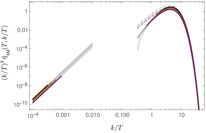
Figure 1: Function $(k/T)^{3}\,\hat{\eta}_{\rm SM}(T,k/T)$ determining the background of stochastic gravitational waves produced in the thermal SM plasma, showing the hydrodynamic contributions (straighter solid lines for smallish $k/T$), the microscopic contributions at full leading order (curved solid lines for higher $k/T$), and their leading-log approximations (dashed lines). The lines are colored for the scales in which the calculations can be trusted, i.e. $k<\alpha^{2}_{1}\,T$ for the hydrodynamic contributions, and $k>m_{\rm 3}(T)$ for the microscopic ones. From top to bottom, the temperatures correspond to $T=10^{3}$ GeV (black), $T=10^{8}$ GeV (red), $T=10^{13}$  GeV (green) and $T=M_{P}$ (violet). The gauge and Yukawa couplings were evaluated at the renormalization $\bar{\mu}=2\pi T$ using the respective two-loop renormalization group equations.

2.3 CGMB in the SM

In the SM we assign $n=1,2,3$ to the gauge groups U(1)_Y, SU(2)_L, SU(3). With the SM matter content one has

$$\begin{aligned} N_{\rm species,SM}=&\,\frac{11}{2},&N_{\rm leptons,SM}=&\,\frac{3}{2},\\ \hat{m}^{2}_{1,\rm SM}(T)=&\,\frac{11}{6}g_{1}(T)^{2},&\hat{m}^{2}_{2,\rm SM}(T)=&\,\frac{11}{6}g_{2}(T)^{2},&\hat{m}^{2}_{3,\rm SM}(T)=&\,2g_{3}(T)^{2}.\end{aligned}$$ (2.51)

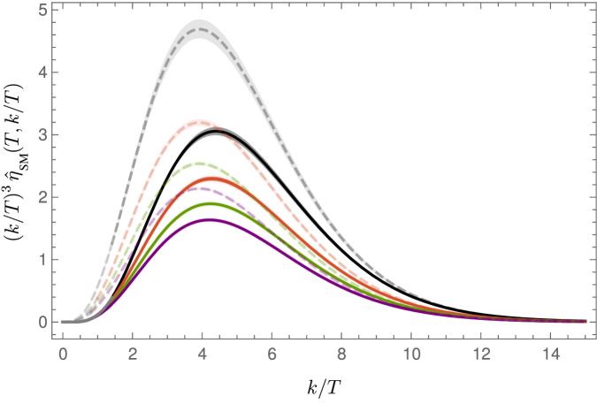
Figure 2: Microscopic contributions to $(k/T)^{3}\,\hat{\eta}_{\rm SM}(T,k/T)$ (solid lines) and their logarithmic approximations (dashed lines). The lines are colored for the scales in which the calculations can be trusted, i.e. $k>m_{\rm D3}(T)$. From top to bottom, the temperatures correspond to $T=10^{3}$ GeV (black), $T=10^{8}$ GeV (red), $T=10^{13}$  GeV (green) and $T=M_{P}$ (violet). The lines are surrounded by bands corresponding to the effect of varying the renormalization scale by a factor of 2 around the central scale $\bar{\mu}=2\pi T$. The maxima of the leading logarithmic approximation occur at $k/T\simeq 3.92$, as anticipated in Eq. (2.27). The maxima of the full leading order approximation are slightly shifted towards higher values.

With this one can fix $\bar{\eta}$ as well as the $\hat{\eta}_{\rm HTL}$ contribution of Eqs. (2.9) and (2.12). Computing as well the coefficients of the loop functions in terms of the representations and couplings in the SM leads to:

$$\hat{\eta}_{\rm SM}\left(T,\frac{k}{T}\equiv\hat{k}\right)\simeq\left\{\begin{array}[]{ll}\displaystyle\frac{15.51}{g_{1}^{4}\ln(5/\hat{m}_{1,\rm SM})},&\;\quad\hat{k}\lesssim\alpha_{1}^{2},\\ \\ \displaystyle\frac{}{}\hat{\eta}_{\rm HTL,SM}(T,\hat{k})+(3g_{2}^{2}+12g_{3}^{2})\eta_{gg}(\hat{k})&\\ \displaystyle\frac{}{}+(g_{1}^{2}+3g_{2}^{2})\eta_{sg}(\hat{k})+(5g_{1}^{2}+9g_{2}^{2}+24g_{3}^{2})\eta_{fg}(\hat{k})&\;\quad\hat{k}\gtrsim{\rm max}\,\{\hat{m}_{n}\}.\\ \displaystyle\frac{}{}+(3|y_{t}|^{2}+3|y_{b}|^{2}+|y_{\tau}|^{2})\,\eta_{sf}(\hat{k}),&\end{array}\right.$$ (2.57)

In the previous equations we omitted for simplicity the logarithmic $T$-dependence of the couplings $g_{i}$, $y_{i}$ and the rescaled Debye masses $\hat{m}_{i}$. We have also ignored the Yukawa couplings of the lightest fermions.

A comparison between the leading-log result of Eq. (2.13) applied to the SM and the complete leading-order contribution in Eq. (2.57) is shown in Figs. 1 and 2. For the calculations we used 2-loop RG equations for the SM couplings in the $\overline{\rm MS}$ scheme [23], supplemented with the $g_{3}$-dependent three-loop contribution to the running of $g_{3}$ [24], evaluated at a temperature-dependent renormalization scale. The couplings were fixed at low scales using values $m_{t}=172.9\,{\rm GeV},m_{h}=125.10\,{\rm GeV}$ for the physical top and Higgs masses. For the determination of $y_{t}$ from the top mass we used one-loop electroweak and three-loop QCD threshold corrections [25, 26, 27], while for computing the Higgs couplings we used the full two-loop effective potential plus appropriate momentum corrections, as in Ref. [28]. We made different choices of the renormalization scale, $\mu=\kappa 2\pi T$ with $\kappa=1/2,1,2$, in order to estimate theoretical uncertainties. Figs.  1 and 2 illustrate how the leading-log result captures the leading-order result quantitatively for $k/T\gtrsim 10$, whereas it overestimates the latter by a factor around two in the phenomenologically most interesting region $k/T\sim 4$. The peak positions of $\hat{k}^{3}\hat{\eta}_{\rm SM}(T,\hat{k})$, on the other hand, are shifted slightly, by less then 10 % from the generic value $\hat{k}_{\rm peak}^{\Omega_{\rm CGMB}}\simeq 3.92$, cf. Eq. (2.27), estimated from the leading-log result. The true peaks correspond to values of $\hat{k}$ slightly about 4, of the order of 4.2 at high temperatures, cf. Fig. 2. The locations of the peaks agree to better than $1$ % accuracy with Eqs. (2.38) and (2.42), specialized to the SM. For the peaks of $\hat{k}\hat{\eta}_{\rm SM}(T,\hat{k})$ – relevant for computing the peak frequency of the characteristic amplitude $h_{c}^{\rm CGMB}$ – we find $\hat{k}^{h_{c}}_{\rm peak}\approx 2.1$. In Fig. 2 we show with colored bands the variations from the change in renormalization scale; these are noticeably smaller in the full-leading order result and remain below 2%.

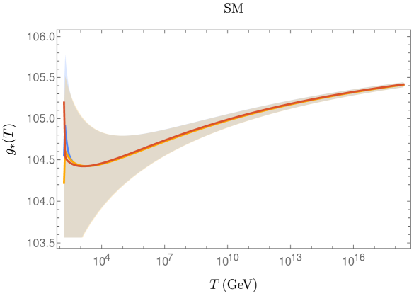
Figure 3: $g^{\rm SM}_{*\rho}(T)$ (blue) $g^{\rm SM}_{*s}(T)$ (orange) and $g^{\rm SM}_{*c}(T)$ (red). The bands show the uncertainties coming from changing the RG scale within a factor of 2 and from shifting the unknown parameter $q_{c}$ of the three-loop QCD corrections to the pressure in Ref. [29] between $-3000$ GeV and $3000$ GeV. The calculation is expected to lose accuracy near the electroweak crossover around 160 GeV. For lower temperatures one should use the results of Refs. [20, 21].

For the computation of the spectrum of thermally produced gravitational waves one has to use Eq. (2.2) and carry out the numerical integration. This requires knowledge of the functions $g_{*\rho}(T)$, $g_{*s}(T)$ and $g_{*c}(T)$. As reviewed in Appendix B, all these quantities can be derived from the thermal corrections to the effective potential –which correspond to minus the pressure of the thermal plasma– and the use of thermodynamical relations. In our calculations we use the full one-loop contributions to the thermal potential, supplemented with three-loop QCD contributions [29]. As we consider gravitational wave production before the electroweak crossover, we can use perturbative results; for lower temperatures one requires more sophisticated techniques [20, 21]. The values used for $g^{\rm SM}_{*\rho}(T)$, $g^{\rm SM}_{*s}(T)$ and $g^{\rm SM}_{*c}(T)$ are shown in Fig. 3.

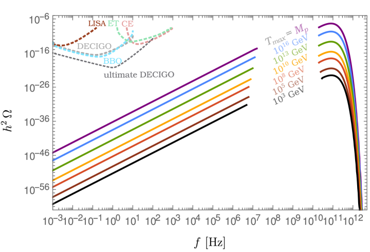
Figure 4: Energy fraction of gravitational waves per logarithmic frequency interval from the primordial thermal plasma in the SM, cf. Eq. (2.2). From top to bottom, the solid lines correspond to the following maximal temperatures: $T_{\rm max}=M_{P}$ (violet), $10^{16}$ GeV (blue), $10^{13}$ GeV (green), $10^{10}$ GeV (orange), $10^{8}$ GeV (red), $10^{5}$ GeV (dark red), $10^{3}$ GeV (black). The dashed lines give the projected sensitivities for planned gravitational wave experiments.

The resulting spectrum of thermally produced gravitational waves is shown in Fig. 4 for different values of the maximum temperature, together with the predicted sensitivities of upcoming gravitational wave experiments like the Big Bang Observer (BBO) [30], the Cosmic Explorer (CE) [31], the Deci-hertz Interferometer Gravitational Wave Observatory (DECIGO) [32], the Einstein Telescope (ET) [33], and LISA [34]. The sensitivity projections were taken from [35]; for ultimate DECIGO we use the curve in Ref. [36] based on Ref. [37].

In Fig. 5 we show the spectra rescaled by $T_{\rm max}$ and compare these results with the analytic approximation (2.2), which predicts a value of $h^{2}\Omega_{\rm CGMB}/T_{\rm max}$ independent of $T_{\rm max}$ aside from variations in $g_{*s}(T_{\rm max})$. The figure shows that the analytic prediction gives results with an accuracy better than 3% near the peak for $T_{\rm max}\gtrsim 10^{5}$ GeV. Within this uncertainty, in accordance with the expectation from Eq. (2.2) the absolute value of $\Omega_{\rm CGMB}(f)$ scales approximately linearly with $T_{\rm max}/M_{P}$. Therefore, a measurement of it determines the maximum temperature of the hot big bang. The peaks in the spectra, for different $T_{\rm max}$, occur around $80$ GHz, less than 10 % higher than the generic estimate (2.28) based on the analytic approximation (2.2) and the leading-log result for $\hat{\eta}(T,\hat{k})$, while they are reproduced with an accuracy of the order of 3% or better (1% or better for $h_{c}^{\rm CGMB}$) by the formulae (2.42) and (2.38).

To end this section, let us note that the theoretical uncertainty of the above results for $h^{2}\Omega_{\rm CGMB}$ in the SM is of the order of 0.1%. This has been estimated by considering the effect of varying the renormalization scale by a factor of 2, and by considering values between -3000 GeV and 3000 GeV of the unknown parameter $q_{c}$ appearing in the three-loop contributions to the QCD pressure of Ref. [29]. Note that the final uncertainty is one order of magnitude lower than the maximal theoretical uncertainties found for $\hat{\eta}$; this is due to cancellations between the variations of $\hat{\eta}$ and the effective numbers of degrees of freedom.

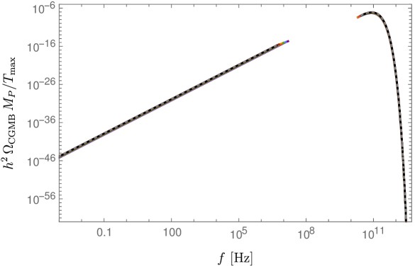
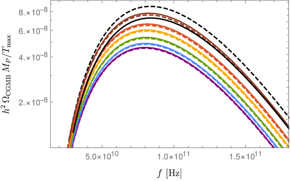
Figure 5: Same spectra as in Fig. 4, multiplied by $M_{P}/T_{\rm max}$. The dashed lines give the results obtained using the simplified formula (2.2).

2.4 CGMB in minimal BSM models explaining neutrino masses, DM, and the BAU

So far, our predictions were based on the assumption that the SM is valid up to the Planck scale, and the value of the temperature $T_{\rm max}$ was left unspecified. However, there is a strong case for BSM physics. It is definitely required to explain neutrino masses and mixing, the origin of the non-baryonic DM, and the BAU. Therefore, we consider now two minimalistic extensions of the SM which solve also these problems. In addition to the latter issues, these models also accommodate realizations of the inflation mechanism, which can address the flatness and horizon problems associated with the observed lack of curvature and the striking homogeneity of the universe. As such, they have all the necessary ingredients to explain the cosmic history of the universe from inflation until the present time; in particular, this means that they give rise to concrete predictions of $T_{\rm max}$ as a result of the post-inflationary reheating dynamics. In turn, this gives refined predictions for the spectrum of gravitational waves originated from the thermal plasma.

The $\nu$MSM [11, 12] extends the SM by three right-handed SM singlet neutrinos, which have a GeV scale Majorana neutrino mass and mix with the three active left-handed neutrinos via Yukawa interactions with the SM Higgs field. This model may be valid up to the Planck scale. Neutrino masses and mixing are generated by the type-I seesaw mechanism [38, 39, 40, 41]. DM is comprised by a keV-scale neutrino mass eigenstate, and the BAU is produced by a low-scale leptogenesis mechanism involving neutrino oscillations [42]. Chaotic inflation can be provided by the Higgs field when allowing for a non-minimal gravitational coupling $S\supset-\int d^{4}x\sqrt{-g}\,\xi_{H}\,H^{\dagger}H\,R$ [43, 44]. The CMB observations require a large, nonperturbative value of $\xi_{H}\sim 4\times 10^{4}\sqrt{\lambda_{H}}$, with $\lambda_{H}$ the Higgs self-quartic. Since the latter is determined by the Higgs mass and VEV, $m_{h}\simeq 125$ GeV, $v\simeq 246$ GeV, as $\lambda_{H}\simeq m_{h}^{2}/2v^{2}$, one has $\lambda_{H}\simeq 0.13$ at low scales, leading to very large values of $\xi_{H}$. For critical scenarios in which the top mass allows a small $\lambda_{H}$ at the high scales relevant for inflation, one may get $\xi_{H}\sim O(10)$ [45, 46]. Values of $\xi_{H}\gtrsim 1$ have been connected with a lack of unitarity [47, 48], yet arguments against this have been given e.g. in [49, 50, 51]. In any case, one may have to pay the prize of uncertain predictions due to unknown nonperturbative corrections to the tree level results. Nevertheless, ignoring this caveat, the tensor-to-scalar ratio $r={\mathcal{P}}_{T}/{\mathcal{P}}_{S}$ and the maximum temperature of the universe in the $\nu$MSM after reheating from Higgs inflation have been determined as [44]

$$r\simeq 0.0034,\hskip 25.83325pt3.4\times 10^{13}\,{\rm GeV}\lesssim T_{\rm max}^{\nu{\rm MSM}}\lesssim 9.3\times 10^{13}\,{\rm GeV}\,\left(\frac{\lambda_{H}}{0.13}\right)^{1/4}\,.$$ (2.58)

These temperatures are much below the absolute upper bound following from the CMB constraint on the tensor-to-scalar ratio, $r<0.058$, and the unphysical assumption of instantaneous and maximally efficient reheating to a radiation dominated universe,

$$T_{\rm max}^{\nu{\rm MSM}}<6.6\times 10^{15}\,{\rm GeV}\,,$$ (2.59)

cf. Appendix C. The thermal plasma of the $\nu$MSM differs from the thermal plasma of the SM only slightly – from the subleading effects of the Yukawas of the singlet neutrinos, that contribute to the $\eta_{sf}$ term in Eq. (2.9) – and therefore the rate of production can be approximated with that in the SM, Eq. (2.57). In regards to the calculation of the present day spectrum using Eq. (2.2), one has to use the values for $g_{*\rho}$, $g_{*s}$, $g_{*c}$ appropriate for the $\nu$MSM. We assume that the singlet neutrinos remain in thermal equilibrium above the electroweak crossover, so that the values of the effective degrees of freedom can be obtained from those of the SM by adding 3 units.

An alternative minimal extension of the SM explaining the origin of DM and the BAU is SMASH [13, 14]. A SM singlet complex scalar field $\sigma$, which features a spontaneously broken global $U(1)_{\rm PQ}$ Peccei-Quinn (PQ) symmetry [53], and a vector-like coloured Dirac fermion $Q$ are added to the field content of the $\nu$MSM. Exploiting the PQ mechanism, this model solves the strong CP problem. DM is comprised by the axion [54, 55, 56] – the pseudo Nambu-Goldstone boson of the $U(1)_{\rm PQ}$ breaking [57, 58] – provided that the PQ breaking scale is in the range $1.3\times 10^{9}\lesssim v_{\sigma}/{\rm GeV}\lesssim 2.2\times 10^{11}$ [59]. The right-handed neutrinos get their Majorana masses also from spontaneous PQ symmetry breaking. The generation of the BAU proceeds via high-scale thermal leptogenesis [60]. Finally, inflation can be accommodated for perturbative values of the non-minimal gravitational couplings [13, 14]. Allowing for a non-minimal coupling $\xi_{\sigma}$ of the PQ field to the Ricci scalar, $S\supset-\int d^{4}x\sqrt{-g}\,\xi_{\sigma}\,\sigma^{*}\sigma\,R$, a mixture of the modulus of the complex PQ field, $\rho=\sqrt{2}\,|\sigma|$, with $h$, the neutral component of the SM Higgs doublet in the unitary gauge, is a viable inflaton candidate. Fitting the inflationary predictions to the observed fluctuations in the CMB relates the size of the non–minimal coupling and the quartic coupling; for the latest Planck data [52] this gives [36]

$$7\times 10^{-3}\lesssim\xi_{\sigma}\simeq 4\times 10^{4}\sqrt{\lambda_{\sigma}}\lesssim 1.$$ (2.60)

The above window was obtained after ensuring a consistent post-inflationary history in which Planck’s CMB pivot scale was matched to the appropriate mode during inflation. The lower bound, $\xi_{\sigma}\gtrsim 7\times 10^{-3}$, arises from taking into account the upper limit on the tensor-to-scalar ratio, $r<0.058$, while the upper bound, $\xi_{\sigma}\lesssim 1$, arises from perturbativity and unitarity requirements. It corresponds to a lower limit on the tensor-to-scalar ratio, $r\gtrsim 4\times 10^{-3}$. As a consequence, the quartic coupling should be in the range $7\times 10^{-13}\lesssim\lambda_{\sigma}\lesssim 5\times 10^{-10}$. The initial conditions for the standard hot big bang cosmology following inflation, non-perturbative preheating and perturbative reheating can be predicted from first principles in SMASH. The maximum temperature of the thermalized SMASH plasma after reheating is obtained as [14]

$$8\times 10^{9}\,{\rm GeV}\lesssim T^{\rm SMASH}_{\rm max}\lesssim 2\times 10^{10}\,{\rm GeV}\,.$$ (2.61)

Again, this is significantly below the upper bound on $T_{\rm max}$ following from the assumption of instant reheating and the CMB constraint $r<0.058$, which in this case gives

$$T_{\rm max}^{\rm SMASH}<6.4\times 10^{15}\,{\rm GeV}\,,$$ (2.62)

In order to calculate the CGMB in SMASH we can use the general expressions of Section 2.1. This requires knowing the BSM Yukawa couplings in SMASH. Stability in the $\sigma$ direction demands small couplings for the RH neutrinos [14], whose effect will be ignored as in the $\nu$MSM; this leaves the Yukawa couplings of the exotic vector quark. Assuming a small interaction with the down quarks (we consider the SMASH realization with hypercharge $1/3$ for $Q$, in which such mixing allows the $Q$s to decay before nucleosynthesis), one has

$${\cal L}\supset y_{Q}\,\sigma\bar{Q}P_{L}Q+c.c..$$ (2.63)

With the matter content in SMASH one has

$$\begin{aligned} N_{\rm species,SMASH}=&\,\frac{35}{6},&N_{\rm leptons,SMASH}=&\,\frac{3}{2},\\ \hat{m}^{2}_{1,\rm SMASH}(T)=&\,\frac{35}{18}\,g_{1}(T)^{2},&\hat{m}^{2}_{2,\rm SMASH}(T)=&\,\frac{11}{6}\,g_{2}(T)^{2},&\hat{m}^{2}_{3,\rm SMASH}(T)=&\,\frac{13}{6}\,g_{3}(T)^{2}.\end{aligned}$$ (2.64)

With this one can fix $\bar{\eta}$ as well as the $\hat{\eta}_{\rm HTL}$ contribution of Eqs. (2.9) and (2.12). Computing as well the coefficients of the loop functions in terms of the representations and couplings in the SM leads to:

$$\hat{\eta}_{\rm SMASH}\left(T,\frac{k}{T}\equiv\hat{k}\right)\simeq\left\{\begin{array}[]{ll}\displaystyle\frac{14.68}{g_{1}^{4}\ln(5/\hat{m}_{1,\rm SMASH})},&\;\quad\hat{k}\lesssim\alpha_{1}^{2},\\ \\ \displaystyle\frac{}{}\hat{\eta}_{\rm HTL,SMASH}(T,\hat{k})+(3g_{2}^{2}+12g_{3}^{2})\eta_{gg}(\hat{k})&\\ \displaystyle\frac{}{}+(g_{1}^{2}+3g_{2}^{2})\eta_{sg}(\hat{k})+\left(\frac{16}{3}g_{1}^{2}+9g_{2}^{2}+28g_{3}^{2}\right)\eta_{fg}(\hat{k})&\;\quad\hat{k}\gtrsim{\rm max}\,\{\hat{m}_{n}\}.\\ \displaystyle\frac{}{}+\left(3|y_{t}|^{2}+3|y_{b}|^{2}+|y_{\tau}|^{2}+\frac{3}{2}|y_{Q}|^{2}\right)\,\eta_{sf}(\hat{k}),&\end{array}\right.$$ (2.70)

For the computation of $g_{*\rho}$, $g_{*s}$, $g_{*c}$ in SMASH we proceed as in Ref. [36]. In order to reliably follow the change in degrees of freedom across the PQ phase transition, one has to use an improved daisy resummation of thermal effects compatible with thermal decoupling. At low temperatures, the SMASH theory is matched to the SM plus the real part of $\sigma$ and the nearly massless axion; we include again three-loop QCD corrections plus corrections from the loss of chemical equilibrium of the axion due to its feeble interactions, which imply that the axion population has a different effective temperature than the rest of the plasma. For details, see Ref. [36]; a summary is given in Appendix B. Figure 6 shows results for $g^{\rm SMASH}_{*\rho}(T)$, $g^{\rm SMASH}_{*s}(T)$ and $g^{\rm SMASH}_{*c}(T)$ for two benchmark points with $r=0.0037$ and $r=0.048$, taken from Ref. [36].

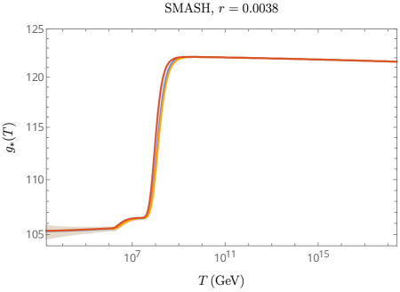
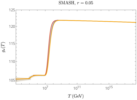
Figure 6: $g^{\rm SMASH}_{*\rho}(T)$ (blue) $g^{\rm SMASH}_{*s}(T)$ (orange) and $g^{\rm SMASH}_{*c}(T)$ (red) for benchmark points with $r=0.0037$ (left) and $r=0.048$ (right). The bands show the uncertainties coming from changing the RG scale within a factor of 2 and from shifting the unknown parameter $q_{c}$ of the three-loop QCD corrections to the pressure in Ref. [29] between $-3000$ GeV and $3000$ GeV. The calculation is expected to lose accuracy near the electroweak crossover around 160 GeV.

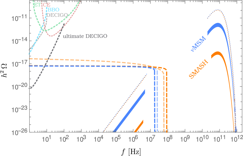
Figure 7: Energy fraction of gravitational waves per logarithmic frequency interval in the $\nu$MSM (blue) and in SMASH (orange). The solid bands correspond to waves sourced from the primordial thermal plasma in the predicted range of reheating temperatures ($3.4\times 10^{13}\,{\rm GeV}\lesssim T^{\nu\rm MSM}_{\rm max}\lesssim 1.1\times 10^{14}\,{\rm GeV}$ for the $\nu$MSM and $8\times 10^{9}\,{\rm GeV}\lesssim T^{\rm SMASH}_{\rm max}\lesssim 2\times 10^{10}\,{\rm GeV}$ for SMASH). The dotted lines give the predictions for the upper bound on the reheating temperature in Eq. (C.3) inferred from current CMB constraints. The dashed lines correspond to waves sourced by inflationary perturbations in the range allowed in each model. For the $\nu$MSM, the darker dashed line corresponds to $r=0.0034$ and $T^{\nu\rm MSM}_{\rm max}=3.4\times 10^{13}\,{\rm GeV}$, while the fainter line corresponds to $r=0.0033,\,T^{\nu\rm MSM}_{\rm max}=10^{14}\,{\rm GeV}$. In SMASH, dark orange corresponds to the minimal value of the tensor-to-scalar-ratio $r=0.0037$, and light orange to the maximum value $r=0.058$.

With the previous results for $\hat{\eta}$, $g_{*\rho}$, $g_{*s}$ and $g_{*c}$, and taking into account the ranges of $T_{\rm max}$ in Eqs. (2.58) and (2.61), one can use Eq. (2.2) to calculate the predictions for the CGMB in the $\nu$MSM and SMASH. As the results for $\hat{\eta}$ assume massless fields, in the SMASH case we use Eq. (2.70) at high temperatures, and the SM result of Eq. (2.57) below the temperature at which the axion field decouples. The latter was estimated as in Ref. [36] by finding the temperature near the critical temperature of the PQ phase transition at which the trace of the stress-energy momentum tensor has a local maximum. The results are shown in Fig. 7, together with the inflationary Cosmic Gravitational Wave Background (iCGWB) due to the tensor modes generated by quantum fluctuations during inflation. For frequencies $f\gtrsim 10^{-16}\,{\rm Hz}$, which re-entered the horizon during radiation domination, the iCGWB can be calculated as [21],

$$\Omega_{\rm iCGWB}(f)\simeq\frac{1}{24}\,\Omega_{\gamma}\left[\frac{g_{*\rho}(T_{\rm hc}(f))}{2}\right]\left[\frac{g_{*s}(T_{\rm hc}(f))}{g_{*s}(\rm fin)}\right]^{-4/3}\,{\cal P}_{T}(f)\,,\hskip 12.91663pt{\rm for}\ f\gtrsim 10^{-16}\,{\rm Hz}\,.$$ (2.71)

In the equation above ${\cal P}_{T}(f)$ is the power spectrum of gravitational waves generated during inflation expressed in terms of the present frequency,

$${\cal P}_{T}(f)=\,\left.\frac{2H_{\rm inf}^{2}}{\pi^{2}M_{P}^{2}}\right|_{a_{\rm inf}H_{\rm inf}=2\pi f},$$ (2.72)

where $a_{\rm inf}$, $H_{\rm inf}$ are the scale factor and Hubble constant during inflation, which we have computed assuming non-critical inflation for the $\nu$MSM and without resorting to the usual slow-roll approximation, but rather by numerically solving the equation of motion for the inflationary background as a function of the number of efolds [61, 14]. $T_{\rm hc}(f)$ in Eq. (2.71) is the temperature at which the mode corresponding to the frequency $f$ re-entered the horizon during radiation domination. It can be obtained by solving [21]

$$T_{\rm hc}(f)=10^{8}{\rm GeV}\times\frac{f}{1.2\,\rm Hz}\times\left[\frac{g_{*s}(\rm fin)}{3.91}\right]^{-1/3}\times[g_{*\rho}(T_{\rm hc}(f))]^{-1/2}\times[g_{*s}(T_{\rm hc}(f)]^{1/3}.$$ (2.73)

The iCGWB has an upper cutoff corresponding to frequencies that never exited the horizon during inflation. We have approximated this by a sharp feature, yet for frequencies near this threshold our calculations beyond the slow-roll approximation already show a drop in the power spectrum, as can be seen in Fig. 7. Note that, for both SMASH and the non-critical $\nu$MSM, the iCGGWB does not overlap with the peak in the CGMB, so that both sources of gravitational waves – inflationary perturbations and thermal processes – become distinguishable if experiments reach the appropriate sensitivity.

In the case of SMASH, the theoretical uncertainty in the calculations of $h^{2}\Omega_{\rm CGMB}/T_{\rm max}$ is of the order of 2%. As before, this quantity corresponds to the variations of the results under changes of the renormalization scale and the unknown three-loop contributions to the QCD pressure.

In our calculations we find that at sufficiently high temperatures $\hat{k}^{3}\hat{\eta}_{\rm SMASH}$ peaks near $\hat{k}^{\Omega}_{\rm peak}\sim 4.2$, and within 1% range of the SM results at the same temperatures. Similarly we get $\hat{k}^{h_{c}}_{\rm peak}\sim 2.1$-2.2, within $1.5\%$ of the corresponding SM results. This means that Eq. (2.48) is satisfied with better than $\sim 1$% accuracy. On the other hand, we find that the relation for $h_{c}$ in Eq. (2.48) is satisfied with better than 4% accuracy. Under the assumption of a SMASH plasma and given a measurement of the peak frequency and the maximum value of $h_{c}^{CGMB}$, then Eqs. (2.47) and (2.48) would allow to estimate $g^{1/3}_{*s}(T_{\rm max})$ and $T_{\rm max}$ within errors around $1\%$ and $5\%$, respectively. Some details of the peak frequencies and amplitudes for several SMASH benchmark points are given in Table 2.

2.5 CGMB in the MSSM

The MSSM goes beyond the SM by adding a fermionic (scalar) superpartners for all the SM bosons (fermions). Additionally, the model contains an extra scalar Higgs doublet with its corresponding fermionic partners.

Given the matter content of the MSSM, and assuming that the scalar partners of the right-handed leptons contribute to $N_{\rm leptons}$ in analogous manner to the usual leptons (i.e. adding the contribution ${1}/{2}\sum_{\hat{i}:T_{n,\hat{i}}=0,n>1}T_{1,\hat{i}}$ to Eq. (2.3)) one obtains:

$$\begin{aligned} N_{\rm species,MSSM}=&\,\frac{33}{2},&N_{\rm leptons,MSSM}=&\,\frac{9}{2},\\ \hat{m}^{2}_{1,\rm MSSM}(T)=&\,\frac{11}{2}g_{1}(T)^{2},&\hat{m}^{2}_{2,\rm MSSM}(T)=&\,\frac{9}{2}g_{2}(T)^{2},&\hat{m}^{2}_{3,\rm MSSM}(T)=&\,\frac{9}{2}g_{3}(T)^{2}.\end{aligned}$$ (2.74)

Computing the coefficients of the loop functions in Eq. (2.9) leads to:

$$\hat{\eta}_{\rm MSSM}\left(T,\frac{k}{T}\equiv\hat{k}\right)\simeq\left\{\begin{array}[]{ll}\displaystyle\frac{16.24}{g_{1}^{4}\ln(5/\hat{m}_{1,\rm MSSM})},&\;\quad\hat{k}\lesssim\alpha_{1}^{2},\\ \\ \displaystyle\frac{}{}\hat{\eta}_{\rm HTL,MSSM}(T,\hat{k})+(3g_{2}^{2}+12g_{3}^{2})\eta_{gg}(\hat{k})&\\ \displaystyle\frac{}{}+(22g_{1}^{2}+42g_{2}^{2}+96g_{3}^{2})\eta_{sg}(\hat{k})\\ \displaystyle\frac{}{}+\left(\frac{11}{2}g_{1}^{2}+\frac{27}{2}g_{2}^{2}+36g_{3}^{2}\right)\eta_{fg}(\hat{k})&\;\quad\hat{k}\gtrsim{\rm max}\,\{\hat{m}_{n}\}.\\ \displaystyle\frac{}{}+(48g_{3}^{2}+21g_{2}^{2}+11g_{1}^{2}\\ \displaystyle\frac{}{}+9|y_{t}|^{2}+9|y_{b}|^{2}+3|y_{\tau}|^{2})\,\eta_{sf}(\hat{k}),&\end{array}\right.$$ (2.82)

Note how in the $sg$ and $fg$ contributions the coefficients in front of the gauge couplings squared are larger than in the previous models, due to the extra matter fields charged under the gauge interactions. Additionally, one has gauge coupling contributions in the coefficient of the loop function $\eta_{sf}$, as a consequence of the fact that supersymmetry implies a relation between the Yukawa couplings of the gauge superpartners and the usual gauge couplings. Analogously, the coefficients of the usual Yukawa couplings are larger than before because supersymmetry relates the usual Yukawa couplings to those of additional interactions involving scalar superpartners.

For our estimates of gravitational wave spectra in the MSSM, we have used the naive value of the effective number of relativistic degrees of freedom,

$$g_{*\rho,\rm MSSM}(T)\approx g_{*s,\rm MSSM}(T)\approx g_{*c,\rm MSSM}(T)\approx 228.75.$$ (2.83)

The reason for this simplification is that we lack knowledge of the QCD corrections to the pressure coming from scalar superpartners. For our numerical estimates we consider a simple scenario in which the dimensionful parameters in the MSSM that are not present in the SM are assumed to lie around the 2 TeV scale. We further assume that the lightest neutral Higgs state is SM-like, which can be realized with a small neutral Higgs mixing angle $\alpha$ (we take $\cot\alpha=10$) and a heavy pseudoscalar Higgs, taken to have a mass of 2 TeV. Demanding the correct mass of the $Z$ boson in the vacuum implies that the ratio of vacuum expectation values for the Higgs doublets $H_{u}$ and $H_{d}$ is $\tan v_{u}/v_{d}=8.5$. Given the SM-like low-energy limit, we evolve the couplings with the two-loop SM RG up to a scale of 2 TeV. At this scale we match the SM to the MSSM by applying appropriate one-loop threshold corrections, and for higher scales we use the 2 loop MSSM RG equations for the gauge and Yukawa couplings [63, 64, 65]. For the calculation of the spectrum of gravitational waves we use Eq. (2.82) at high temperatures, and the SM result of Eq. (2.57) below 2 TeV.

We give MSSM results for the peak frequencies and amplitudes in some benchmark points in Table 2. In the MSSM, the values for $\hat{k}^{\Omega}_{\rm peak,MSSM}(T_{\rm max})$ for high temperatures lie around 4.40, within 5% of their SM counterparts. Analogously, one has $\hat{k}^{h_{c}}_{\rm peak,MSSM}(T_{\rm max})\approx 2.1$-2.2, within 15% of the SM values for the same temperatures. We thus find that Eq. (2.47) holds with an accuracy better than 15%, while the relation for $h_{c}$ in Eq. (2.48) holds up to deviations that remain below 30%. Asuming an MSSM plasma and a hypothetical measurement of the peak frequency and the maximum value of $h_{c}^{\rm CGMB}$, then we find that Eqs. (2.47) and (2.48) would allow to estimate $g^{1/3}_{*s}(T_{\rm max})$ and $T_{\rm max}$ within deviations below 5% and 40%, respectively.

3 Observational constraints on the CGMB

3.1 Dark radiation constraint on the CGMB

The CGMB acts as an additional dark radiation field in the universe. Any observable capable of probing the expansion rate of the universe, and hence its energy density, has therefore the potential ability to constrain the CGMB energy density ${\rho_{\rm CGMB}}$ present in that moment. BBN and the process of photon decoupling of the CMB yield a very precise measurement of $H$, when the universe had a temperature of $T_{\rm BBN}\sim 0.1$ MeV and $T_{\rm CMB}\sim 0.3$ eV, respectively. A constraint on the presence of ‘extra’ radiation is usually expressed in terms of an extra effective number of neutrinos species, $\Delta N_{\nu}$,

$$\Delta\rho_{\mathrm{rad}}(T)=\frac{\pi^{2}}{30}\,\frac{7}{4}\,\Delta N_{\nu}\,T^{4}\,.$$ (3.1)

Since the energy density in the CGMB must satisfy $\rho_{\rm CGMB}(T)\leq\Delta\rho_{\mathrm{rad}}(T)$, one finds a constraint on the CGMB energy density redshifted to today in terms of the number of extra neutrino species,

$$h^{2}\,\int\limits_{0}^{\infty}\frac{{\rm d}f}{f}\,\Omega_{\rm CGMB}(f)=h^{2}\,\frac{\rho_{\rm CGMB}^{(0)}}{\rho_{c}^{(0)}}\leq h^{2}\Omega_{\gamma}\left(\frac{g_{*s}({\rm fin})}{g_{*s}(T)}\right)^{4/3}\frac{7}{8}\,\Delta N_{\nu}\simeq 5.7\times 10^{-6}\,\Delta N_{\nu}\,,$$ (3.2)

where $\rho_{c}^{(0)}=3H_{0}^{2}M_{P}^{2}$, and we have used $g_{*s}({\rm fin})\simeq 3.931$ and $g_{*s}(T=\mathrm{MeV})\approx 10.75$. This bound corresponds roughly to a direct bound on the CGMB energy fraction per logarithmic frequency interval,

$$h^{2}\,\Omega_{\rm CGMB}(f)\lesssim h^{2}\,\Omega_{\rm CGMB}(f_{\rm peak}^{\Omega_{\rm CGMB}})<5.7\times 10^{-6}\,\Delta N_{\nu}\,,$$ (3.3)

because it has a large width of order the peak frequency itself.

The latest BBN constraints on $\Delta N_{\nu}$ can be found in Ref. [66]. The ${}^{4}\mathrm{He}$ alone is not very constraining due to degeneracies with the baryon-to-photon ratio $\eta_{B}$, so that the best constraints come from combining BBN measurements of ${}^{4}\mathrm{He}$ and deuterium abundances with CMB results. In this case Ref. [66] finds $\Delta N_{\nu}<0.3$ at 95% implying, from Eq. (3.2), $h^{2}\,\rho_{\rm CGMB}^{(0)}/\rho_{c}^{(0)}<1.7\times 10^{-6}$.

A similar bound is obtained from other inferences from CMB [67, 68, 69]. In particular, the analysis of Ref. [69] uses Planck data, together with CMB lensing, baryon acoustic oscillations and also deuterium abundances, and finds a constraint that goes down to

$$h^{2}\,\rho_{\rm CGMB}^{(0)}/\rho_{c}^{(0)}<1.2\times 10^{-6}.$$ (3.4)

Not surprisingly, this is comparable to what is obtained from the BBN analysis in Ref. [66], which also uses CMB data to pin down the baryon to photon ratio $\eta_{B}$. However, Ref. [69] only analyses adiabatic initial conditions. From the results of Refs. [67, 68], one can infer that there is a gain when imposing homogeneous initial conditions, due to the breaking of degeneracies with neutrino parameters [22]. This has been confirmed by Ref. [70], which under the hypothesis of GW with homogeneous initial conditions finds

$$h^{2}\,\rho_{\rm CGMB}^{(0)}/\rho_{c}^{(0)}<2.9\times 10^{-7}\,.$$ (3.5)

Finally, it should be noted that, in the CMB context, the bound in Eq. (3.2) is often quoted in terms of $\Delta N_{\rm eff}$, the effective number of extra neutrino species present in the thermal bath after $e^{+}e^{-}$ annihilation. In this case, instead of normalising at $T={\rm MeV}$, one can choose a temperature below $e^{+}e^{-}$ annihilation, leading to a bound equivalent to Eq. (3.2),

$$h^{2}\,{\rho_{\rm CGMB}^{(0)}}/{\rho_{c}^{(0)}}\leq h^{2}\Omega_{\gamma}({7}/{8})\,\left({4}/{11}\right)^{4/3}\Delta N_{\rm eff}\simeq 5.6\times 10^{-6}\,\Delta N_{\rm eff}\,.$$ (3.6)

The current theoretical uncertainty of $\Delta N_{\rm eff}$ is of the order of $10^{-3}$  [71, 72, 73, 74]. If experiments were to reach this level of precision, one would obtain an upper bound of $h^{2}\,\rho_{\rm CGMB}^{(0)}/\rho_{c}^{(0)}<5.6\times 10^{-9}$.

	SM	$\nu$MSM	SMASH	MSSM
$T_{\rm max}$ [GeV] $<$	$(1.2$-$5.1)\times 10^{19}$	$(1.3$-$5.4)\times 10^{19}$	$(1.4$-$6.0(1))\times 10^{19}$	$(2.3$-$9.4)\times 10^{19}$
$T^{\Delta N_{\rm eff}=0.001}_{\rm max}$ [GeV] $<$	$2.3\times 10^{17}$	$2.4\times 10^{17}$	$2.7\times 10^{17}$	$4.39\times 10^{17}$

Table 1: Values of the maximal temperature allowed by the dark radiation constraints of Eqs. (3.5)- (3.4), as well as the bound assuming $\Delta N_{\rm eff}$ equal to the theoretical uncertainty of $10^{-3}$. In the case of SMASH the numbers between brackets reflect the change in the last significant digit coming from choosing benchmark scenarios with different values of the tensor-to-scalar ratio. The results for trans-Planckian temperatures are not physically meaningful, as for $T>M_{P}$ one expects early-time equilibration of gravitons and a spectrum as in Eq. (2.49). We list the trans-Planckian temperatures simply to illustrate the reach of current dark radiation bounds.

	$T_{\rm max}$ [GeV]	$f^{\Omega_{\rm CGMB}}_{\rm peak}$ [GHz]	$f^{h^{\rm CGMB}_{c}}_{\rm peak}$ [GHz]	$h^{2}\Omega_{\rm CGMB}(f^{\Omega_{\rm CGMB}}_{\rm peak})$	$h^{\rm CGMB}_{c}(f^{h^{\rm CGMB}_{c}}_{\rm peak})$
SM	$>M_{P}$	74.45	30.26	2.27$\times 10^{-7}$	1.17$\times 10^{-32}$
	2.3$\times 10^{17}$	80.09	40.48	4.47$\times 10^{-9}$	1.42$\times 10^{-33}$
	6.6$\times 10^{15}$	80.23	40.69	1.34$\times 10^{-10}$	2.45$\times 10^{-34}$
	$>M_{P}$	73.75	29.98	2.19$\times 10^{-7}$	1.16$\times 10^{-32}$
$\nu$MSM	2.4$\times 10^{17}$	79.34	40.10	4.43$\times 10^{-9}$	1.43$\times 10^{-33}$
	6.6$\times 10^{15}$	79.48	40.32	1.27$\times 10^{-10}$	2.41$\times 10^{-34}$
	(3.4-11)$\times 10^{13}$	79.73-79.67	40.69-40.60	(7.02-22.34)$\times 10^{-13}$	(1.78-3.19)$\times 10^{-35}$
	$>M_{P}$	70.99	28.85	1.88$\times 10^{-7}$	1.11$\times 10^{-32}$
SMASH	2.7$\times 10^{17}$	76.72	38.98	4.40$\times 10^{-9}$	1.47$\times 10^{-33}$
(r=0.0037)	6.4$\times 10^{15}$	76.83	39.18	1.09$\times 10^{-10}$	2.30$\times 10^{-34}$
	(8-20)$\times 10^{9}$	77.56-77.44	40.35-40.22	(1.64-4.02)$\times 10^{-16}$	(2.79-4.37)$\times 10^{-37}$
	$>M_{P}$	71.06	28.88	1.89$\times 10^{-7}$	1.11$\times 10^{-32}$
SMASH	2.7$\times 10^{17}$	76.81	39.04	4.45$\times 10^{-9}$	1.48$\times 10^{-33}$
(r=0.05)	6.4$\times 10^{15}$	76.91	39.24	1.10$\times 10^{-10}$	2.31$\times 10^{-34}$
	(8-20)$\times 10^{9}$	77.57-77.49	40.39-40.28	(1.65-4.06)$\times 10^{-16}$	(2.79-4.39)$\times 10^{-37}$
	$>M_{P}$	57.50	23.37	8.09$\times 10^{-8}$	9.02$\times 10^{-33}$
MSSM	4.4$\times 10^{17}$	64.75	36.29	4.60$\times 10^{-9}$	1.72$\times 10^{-33}$
	5.5$\times 10^{15}$	64.87	36.48	5.76$\times 10^{-10}$	1.92$\times 10^{-34}$

Table 2: Values of peak frequencies and peak power spectra for the gravitational waves produced from the thermal plasma, for different models and maximum temperatures related to dark radiation and inflationary bounds, or to direct estimates of the reheating temperature. For a given model, the upper row corresponds to temperatures above the Planck mass, for which gravitons are expected to reach thermal equilibrium at early times, leading to an energy fraction around the dark radiation bound of Eq. (3.5). The temperature in the second row is the upper bound corresponding to a hypothetical constraint $\Delta N_{\rm eff}=10^{-3}$. In the third row one has the temperature bound of Eq. (C.4), which applies under the assumption of slow-roll inflation. If present, the range of $T_{\rm max}$ in the fourth row corresponds to direct estimates of the reheating temperature.

We have turned the above limits into upper bounds on $T_{\rm max}$ for the SM, the $\nu$MSM, SMASH and the MSSM, cf. Table 1. The observational limits of Eqs. (3.4) and (3.5) give bounds of the order of $10^{19}$ GeV. These correspond to temperatures above the Planck scale, for which the gravitons can be expected to enter thermal equilibrium and the calculations based on Eq. (2.9) cannot be applied. Thus the previous dark radiation bounds cannot reliably constrain $T_{\rm max}$. For trans-Planckian temperatures one has to use the equilibrium form (2.49) for the CGMB spectrum; integrating over the frequency so as to obtain the total energy fraction gives

$$h^{2}\,\frac{\rho_{\rm Eq.CGMB}^{(0)}}{\rho_{c}^{(0)}}=\left(\frac{g_{*s}({\rm fin})}{g_{*s}(M_{P})}\right)^{4/3}\frac{h^{2}\pi^{2}T_{0}^{4}}{45H_{0}^{2}M_{P}^{2}}=3.0\times 10^{-7}\,\left(\frac{106.75}{g_{*s}(M_{P})}\right)^{4/3}.$$ (3.7)

Intriguingly, this just about saturates the current dark radiation bound obtained assuming homogeneous initial conditions, Eq. (3.5). Note that, in the case of early time equilibration of gravitational waves, one expects in fact homogeneity, and thus the relevant dark radiation bound is indeed given by Eq. (3.5) instead of (3.4). Thus the current dark radiation bound is just on top of the value that corresponds to the contribution from gravitational waves that were in equilibrium at early times. Taking the significant digits of the bound of Eq. (3.5) seriously, then the result of Eq. (3.7) would imply that current dark radiation bounds are compatible with a CGMB with early time equilibrium in an extension of the SM in which $g_{*s}$ is augmented by a few degrees of freedom ($\Delta g_{*s}>2.8$ taking the naive value $g_{*s,{\rm SM}}=106.75$, $\Delta g_{*s}>4$ when including additional radiative corrections as summarized in Appendix B (see Fig. 3)).

The next generation of CMB experiments is expected to improve the sensitivity on $\Delta N_{\rm eff}$ by one order of magnitude. Correspondingly, the upper bound on $T_{\rm max}$ may decrease by a factor of ten and thus reach the reduced Planck scale in the next decade. If future experiments were to reach the theoretical uncertainty $\Delta N_{\rm eff}\sim 10^{-3}$, then one would probe $T_{\rm max}$ at scales of the order of $10^{17}$ GeV, as was already emphasized in Ref. [9]. Note that $T_{\rm max}$ bounds increase for models with more degrees of freedom, as expected from the scaling of Eq. (2.48). More details for the peak frequencies and values of $\Omega_{\rm CGMB}$, $h_{c}^{\rm CGMB}$ for the maximal temperatures that follow from the dark radiation bounds are given in Table 2.

3.2 CMB Rayleigh-Jeans tail constraint on the CGMB

In the presence of magnetic fields, GWs are converted into electromagnetic waves (EMWs) and vice versa. This is called the (inverse) Gertsenshtein effect [75, 76, 77, 78, 79]. Recently, it has been shown that this conversion results in a distortion of the CMB, which can act therefore as a detector for MHz to GHz GWs generated before reionization [80]. The measurements of the radio telescope EDGES have been turned into the bound

$$h_{c}^{\rm CGMB}(f\approx 78\,{\rm MHz})<10^{-12}\,(10^{-21})\,,$$ (3.8)

for the weakest (strongest) cosmic magnetic fields allowed by current astrophysical and cosmological constraints. Similarly, the observations of ARCADE 2 imply

$$h_{c}^{\rm CGMB}(3\,{\rm GHz}\lesssim f\lesssim 30\,{\rm GHz})<10^{-14}\,(10^{-24})\,.$$ (3.9)

These upper bounds are displayed in Fig. 8 as green exclusion regions. Future advances in radio astronomy and a better knowledge of cosmic magnetic fields are required in order that this method can get competitive with the dark radiation constraint.

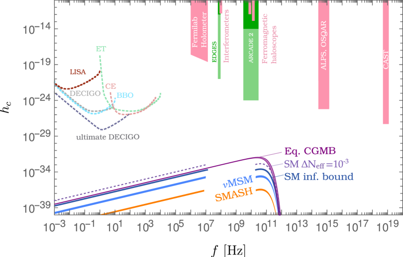
Figure 8: The current upper bounds on the characteristic amplitude $h_{c}$ of a stochastic GW background from direct GW detection experiments (in red) and from the CMB Rayleigh-Jeans tail constraint (in green). Also shown are the projected sensitivities of planned laser interferometers and the predicted amplitudes of the CGMB, for the following five cases (from top to bottom at peak emission): i) CGMB with early time equilibration, in a band of models going from the SM to the MSSM, and corresponding to initial temperatures above the Planck mass and an approximate saturation of the bound of Eq. (3.5), ii) SM plasma with $T_{\rm max}=2.3\times 10^{17}$ GeV (corresponding to $\Delta N_{\rm eff}=10^{-3}$), iii) SM plasma with $T_{\rm max}=6.6\times 10^{15}$ GeV (upper limit consistent with slow-roll inflation, cf. (C.4)), iv) $\nu$MSM plasma with $3.4\times 10^{13}\,{\rm GeV}\lesssim T_{\rm max}^{\nu\rm MSM}\lesssim 1.1\times 10^{14}\,{\rm GeV}$, and v) SMASH plasma with $8\times 10^{9}\,{\rm GeV}\lesssim T_{\rm max}^{\rm SMASH}\lesssim 2\times 10^{10}$ GeV (predicted by (pre-)heating in SMASH [13, 14]).

4 Laboratory searches for the CGMB

In this section we will discuss current constraints on the CGMB from direct experimental GW searches in the laboratory and future possibilities to search for a stochastic GW background in the frequency range around the peak.

4.1 Current direct bounds from GW experiments

Current large-size ground-based laser-interferometric GW detectors, such as GEO, KAGRA, LIGO, and VIRGO [81, 82, 83, 84], are sensitive in the frequency range from about 10 Hz to 10 kHz. Their technology is not necessarily ideal for studying very-high-frequency (VHF: 100 kHz$~{}-1$ THz) and ultra-high-frequency (UHF: above $1$ THz) GWs. Several other small-size experiments have performed pioneering searches for stochastic GWs in the VHF and UHF range and put corresponding upper bounds which are confronted in Fig. 8 to the CGMB prediction:

• A cavity/waveguide prototype experiment searched for polarization changes of electromagnetic waves, which are predicted to rotate under an incoming GW [85]. It provided an upper limit, $h_{c}<1.4\times 10^{-10}$, on the characteristic amplitude of stochastic GWs at 100 MHz.

• Two laser interferometers with $0.75$ m long arms have been set-up as a so-called synchronous recycling interferometer [86]. They provided an upper limit, $h_{c}<1.4\times 10^{-12}$, on the amplitude of a stochastic GW background at 100 MHz [87].

• The Fermilab Holometer, consisting of separate, yet identical Michelson interferometers, with $39$ m long arms, has performed a measurement at slightly lower frequencies. The upper limits, within 3$\sigma$, on the characteristic amplitude of stochastic GWs, are in the range $h_{c}<25\times 10^{-19}$ at 1 MHz down to a $h_{c}<2.4\times 10^{-19}$ at 13 MHz [88].

• Planar GWs induce resonant spin precession of electrons [89, 90]. The same resonance is caused by coherent oscillation of hypothetical axion dark matter [91]. Recently, searches for resonance fluorescence of magnons induced by axion dark matter have been performed and upper bounds on the axion-electron coupling constant have been obtained [92, 93]. These bounds can be translated to bounds on the amplitude of stochastic GWs: $h_{c}\lesssim 1.3\times 10^{-13}$ at 14 GHz and $h_{c}\lesssim 1.1\times 10^{-12}$ at 8.2 GHz [89, 90].

• As mentioned earlier, in an external magnetic field, GWs partially convert into EMWs [75, 76, 77, 78, 79], which can be processed with standard electromagnetic techniques and detected [94], for example, by single-photon counting devices at a variety of wavelengths, cf. Fig. 9. The authors of Ref. [95] used data from existing facilities that have been constructed and operated with the aim of detecting axions or axion-like particles by their partial conversion into photons in magnetic fields: the light-shining-through-walls (LSW) experiments ALPS [96, 97] and OSQAR [98, 99], and the helioscope CAST [100, 101]. They excluded GWs in the frequency bands from $\left(2.7-14\right)\times 10^{14}$ Hz and $\left(5-12\right)\times 10^{18}$ Hz down to a characteristic amplitude of $h_{c}<6\times 10^{-26}$ and $h_{c}<5\times 10^{-28}$, at 95% confidence level, respectively. Using suitable EMW detectors sensitive to $h_{c}$ around its peak value at $\sim 40$ GHz one may exploit such axion experiments also for the search of the CGMB, as we will show in the next subsection.

In summary: all the current upper bounds on the characteristic amplitude of stochastic GWs from direct experimental searches are many orders of magnitude above the CGMB predictions.

4.2 Prospects of EM detection of the CGMB in the laboratory

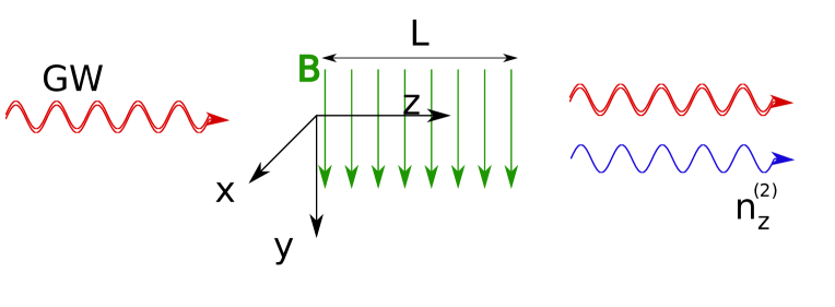
Figure 9: Illustration of the inverse Gertsenshtein effect [75]. If a GW of frequency $f$ passes in vacuum through a transverse static magnetic field of strength $B$, an EMW is produced in the same direction and with the same frequency. Its EM power, at the terminal position of the magnetic field ($z=L$), is proportional to $f^{2}h_{c}^{2}(BL)^{2}$.

In this subsection, we will discuss the prospects of magnetic GW-EMW conversion experiments to probe the CGMB. We will first concentrate on GW-EMW conversion in available static magnetic fields in vacuum with dedicated detectors appropriate for the tens of GHz range and then proceed to a proposal exploiting an additional VHF EM Gaussian beam in order to generate a conversion signal which is first order in $h_{c}$.

4.2.1 Magnetic GW-EMW conversion in vacuum

In this subsection, we consider experiments exploiting the pure inverse Gertsenshtein effect [75], cf. Fig. 9. To this end, we assume that stochastic GWs of amplitude $h_{c}$ propagate through a transverse and constant magnetic $B$ in an evacuated tube of length $L$ and cross-section $A$ for a time $\Delta t$. Then the average power of the generated EMW, per logarithmic frequency interval, at the terminal position of the magnetic field ($z=L$ in Fig. 9) is obtained as [76, 78, 94, 95]

$$f\frac{{\rm d}P^{(2)}_{\rm EMW}}{{\rm d}{f}}\simeq\pi^{2}\,f^{2}\,h_{c}^{2}(f)\,B^{2}\,L^{2}\,A=4.20\times 10^{-23}\,{\rm W}\left[\frac{f}{\rm 40\,GHz}\right]^{2}\,\left[\frac{h_{c}(f)}{10^{-21}}\right]^{2}\,\left[\frac{B}{\rm T}\right]^{2}\,\left[\frac{L}{\rm m}\right]^{2}\,\left[\frac{A}{\rm m^{2}}\right]\\ \,.$$ (4.1)

The index “2” denotes here the fact that the generated EMW power is second order in $h_{c}$. The associated expected average number of generated photons, per unit logarithmic frequency interval, is given by

$$f\frac{{\rm d}N^{(2)}_{z}}{{\rm d}{f}}\simeq\frac{\pi}{2}\,f\,h_{c}^{2}(f)\,B^{2}\,L^{2}\,A\,\Delta t=1.59\left[\frac{f}{\rm 40\,GHz}\right]\,\left[\frac{h_{c}(f)}{10^{-21}}\right]^{2}\,\left[\frac{B}{\rm T}\right]^{2}\,\left[\frac{L}{\rm m}\right]^{2}\,\left[\frac{A}{\rm m^{2}}\right]\,\left[\frac{\Delta t}{{\rm s}}\right]\,.$$ (4.2)

These expressions are valid as long as the GWs and the generated EMWs are in phase coherence throughout their propagation in the magnetic field region. Under the assumption that the external B-field is surrounded by a circular beam tube of diameter $d$, coherent EMW generation is guaranteed if (see Appendix D):

$$f\gg f_{c}\equiv\frac{c_{11}}{\pi^{2}}\frac{L}{d^{2}}\simeq 5.5\times 10^{7}\,{\rm Hz}\,\left[\frac{L}{\rm m}\right]\,\left[\frac{\rm m}{d}\right]^{2},$$ (4.3)

where $c_{11}=1.8$ and $d$ is the diameter of the beam tube. This effective lower frequency cut-off arises from the fact that the evacuated beam tube acts as an EM waveguide, in which the phase velocity of the EMW is higher than the phase velocity of light in vacuum, $v_{\rm EMW}=1/\sqrt{1-(f_{c}/f)^{2}}$

Around the peak frequency of the $h_{c}$ spectrum, $f_{\rm peak}^{h_{c}^{\rm CGMB}}\sim 30-40$ GHz (see Table 2), one may either use heterodyne (HET) radio receivers or single photon detectors (SPDs) to search for an EM signal that was generated from magnetic conversion of the CGMB.

The sensitivity of the HET technique is limited by thermal noise in amplifiers and mixers (for an introduction, see Ref. [103]). In this context, it is useful to introduce an effective signal noise temperature $T_{\rm S}$ equal to the power of the generated EMW in a frequency bin $\Delta f$ around the peak frequency,

$$T_{\rm S}=\frac{\Delta P^{\rm{(2)}}_{\rm EMW}}{\Delta f}\,.$$ (4.4)

Exploiting linear amplifiers with system noise temperature $T_{\rm sys}$, the signal-to-noise ratio is determined then by [103]

$$\frac{\rm S}{\rm N}=\frac{T_{\rm S}}{T_{\rm sys}}\frac{1}{K_{\rm rec}}\sqrt{\Delta f\,\Delta t}\,,$$ (4.5)

where $\Delta f$ is the pre-detection bandwidth of the receiver, $\Delta t$ is the measurement time, and $K_{\rm rec}$ is a receiver-system dependent dimensionless constant of order one From this, we obtain the sensitivity of a magnetic GW-EMW conversion experiment with a heterodyne radiowave receiver to the CGMB as

$$\left[h^{\rm CGMB}_{c}\right]_{\rm sens}^{\rm HET} \simeq 9.65\times 10^{-21}\,\left[\frac{{\rm S}/{\rm N}}{2}\right]^{1/2}\,\left[\frac{\Delta t}{\rm\pi\times 10^{7}\ s}\right]^{-1/4}\,\left[\frac{f}{\rm 40\ GHz}\right]^{-3/4}\,\left[\frac{\Delta f}{f}\right]^{-1/4}\,\times$$ (4.6)

$$\hskip 43.05542pt\times K_{\rm rec}^{1/2}\,\left[\frac{T_{\rm sys}}{\rm 4\,K}\right]^{1/2}\,\left[\frac{B}{\rm T}\right]^{-1}\,\left[\frac{L}{\rm m}\right]^{-1}\,\left[\frac{A}{\rm m^{2}}\right]^{-1/2}\,.$$

	$B$ [T]	$L$ [m]	$d$ [m]	ntubes	$BLA^{1/2}$	$f_{c}$ [Hz]	$[h^{\rm CGMB}_{c}]^{\rm HET}_{\rm sens}$	$[h^{\rm CGMB}_{c}]^{\rm SPD}_{\rm sens}$
ALPS IIc	5.3	211	0.05	1	$49.6$ Tm2	$4.6\times 10^{12}$	–	–
BabyIAXO	2.5	10	0.7	2	$21.9$ Tm2	$1.1\times 10^{9}$	$4.41\times 10^{-22}$	$3.52\times 10^{-25}$
MADMAX	4.83	6	1.25	1	$32.1$ Tm2	$1.9\times 10^{8}$	$3.01\times 10^{-22}$	$2.40\times 10^{-25}$
IAXO	2.5	20	0.7	8	$87.7$ Tm2	$2.2\times 10^{9}$	$1.10\times 10^{-22}$	$8.79\times 10^{-26}$

Table 3: Parameters of the magnetic field regions of ALPs IIc [104, 105], MADMAX [106, 107], BabyIAXO and IAXO [108], used to estimate the minimum detectable GW amplitude through magnetic conversions of GWs (gravitons) to EMWs (photons) in vacuum: $B$ is the magnetic field magnitude, $L$ is the magnetic field length, $d$ is the diameter of the magnetized tube, and $BLA^{1/2}$, with $A=n_{\rm tubes}\pi d^{2}/4$, is the figure of merit for GW detection by magnetic conversion into EMWs. Also shown are the effective lower frequency cut-off Eq. (4.3) and the projected CGMB sensitivities around $f=40\ {\rm GHz}$, exploiting these magnetic field regions and the benchmark values in Eqs. (4.6) and (4.10). ALPS IIc is not sensitive to the CGMB, because the lower frequency cut-off of its magnetic field region is around 5 THz.

The figure of merit of the magnetized region for conversion of GWs into EMWs is $BLA^{1/2}$, cf. Eq. (4.6). This is shared also by LSW experiments exploiting optical cavities at the generation and regeneration side of the experiment and helioscopes searching for the magnetic conversion of axions into photons or vice versa. In Table 3 we show the parameters of the magnetic field region of the next generation of axion experiments: the LSW experiment ALPS IIc [104, 105], the haloscope MADMAX [106, 107], and the helioscopes BabyIAXO and IAXO [108]. Unfortunately, the prospects to probe the CGMB exploiting these magnetic conversion facilities appear to be rather slim. For example, collecting the signal from all eight magnetized tubes of IAXO with a heterodyne radio receiver in a one year CGMB-EMW conversion experiment, the projected sensitivity given in Table 3, $[h^{\rm CGMB}_{c}(f\approx 40\,{\rm GHz})]^{\rm HET}_{\rm sens}\approx 1.10\times 10^{-22}$, is about ten orders of magnitude above the CGMB predictions with early time equilibration, corresponding to initial temperatures above the Planck mass and an approximate saturation of the bound of Eq. (3.5), cf. Fig. 10.

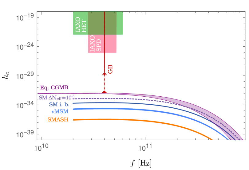
Figure 10: Characteristic amplitude $h_{c}$ of the CGMB (2.33) as in Fig. 8, but focusing on the frequency range near the peak and showing the predicted reach for experiments detecting GW-EMW conversions using heterodyne or single photon detectors in a static magnetic field, or resorting to an additional high-power 40 GHz EM Gaussian beam. The dashed line shows an optimistic projection for the Gaussian beam technique accounting for future technological improvements, see main text.

The prospects are slightly better if progress is made on single photon detection at photon energies around $\omega=2\pi f=1.65\times 10^{-4}\,{\rm eV}[f/40\,{\rm GHz}]$. The signal-to-noise ratio is given in this case by

$$\frac{\rm S}{\rm N}=\frac{\Delta N_{\rm S\,counts}}{\sqrt{\Delta N_{\rm D\,counts}}}\,.$$ (4.7)

Here,

$$\Delta N_{\rm S\,counts}\simeq\epsilon\,\frac{\pi}{2}\,h_{c}^{2}(f)\,B^{2}\,L^{2}\,A\,\Delta t\,\Delta\omega\,,$$ (4.8)

denotes the number of signal counts in a time interval $\Delta t$ and an energy interval $\Delta\omega=2\pi\Delta f$ (cf. Eq. (4.2)), with $\epsilon$ being the single photon detection efficiency and

$$\Delta N_{\rm D\,counts}\simeq\Gamma_{\rm D}\,\Delta t$$ (4.9)

the number of dark counts, in terms of the dark count rate $\Gamma_{\rm D}$. The sensitivity of a magnetic GW-EMW conversion experiment with an SPD detection system is then

$$\left[h^{\rm CGMB}_{c}\right]_{\rm sens}^{\rm SPD} \simeq 7.71\times 10^{-24}\,\left[\frac{{\rm S}/{\rm N}}{2}\right]^{1/2}\,\left[\frac{\Delta t}{\rm\pi\times 10^{7}\ s}\right]^{-1/4}\left(\frac{\Delta\omega}{\rm 10^{-4}\,eV}\right)^{-1/2}\times$$ (4.10)

$$\hskip 43.05542pt\times\epsilon^{-1/2}\,\left[\frac{\Gamma_{\rm D}}{10^{-3}\,\text{Hz}}\right]^{1/4}\,\left[\frac{B}{\rm T}\right]^{-1}\,\left[\frac{L}{\rm m}\right]^{-1}\,\left[\frac{A}{\rm m^{2}}\right]^{-1/2}\,.$$

If the experimental benchmark values chosen in Eq. (4.10) can be reached, the SPD sensitivity is about three orders of magnitude better than the HET sensitivity. However, it is fair to say that, from today’s perspective, vacuum magnetic GW-EMW conversion experiments will fail to beat the dark radiation constraint on $h_{c}^{\rm CGMB}$ by more than six orders of magnitude, cf. Table 3 and Fig. 10.

4.2.2 Magnetic GW-EMW conversion in a VHF EM Gaussian beam

The signal for magnetic GW-EMW conversion in vacuum, such as the generated EM power (4.1) or the number of generated photons (4.2), is of second order in the tiny amplitude $h_{c}$ of the passing GWs. A number of modified schemes have been proposed which introduce in the magnetic conversion region certain powerful auxiliary EM fields oscillating at the frequency of the gravitational wave, such as plane EMWs [113] or EM Gaussian beams (GBs) [114], to obtain GW-induced EMWs which are first order in $h_{c}$. For $h_{c}\ll 1$, their signal strength overwhelms the one from the second order EMWs induced by the inverse Gertsenshtein effect. However, this does not mean automatically that the sensitivity of these modified magnetic conversion experiments is much larger than the one of the experiments based on the inverse Gertsenshtein effect in vacuum, because the powerful auxiliary EMWs tend to increase the noise floor and consequently to decrease the signal-to-noise ratio.

The arguably most promising of these modified magnetic GW-EMW conversion detection proposals exploits a VHF EM GB to induce a first order signal in magnetic GW-EMW conversion [114, 115, 116, 117, 118, 119, 120, 121, 122, 124, 123, 125, 126, 127]. A continuous traveling wave EM GB with frequency $f_{0}$, propagating in the $z$-direction with linear polarization along the $x$-direction, passes through a transverse static magnetic field, cf. Fig. 11. If a GW of frequency $f=f_{0}$ propagates along the $z$-direction, the resonant interaction of the GW with the EM fields of the GB and the static magnetic field will not only generate a longitudinal first order photon flux (denoted by $n_{z}^{(1)}$ in Fig. 11), which will be swamped by the background EM flux $n_{z}^{(0)}$ from the GB, but also a transverse first order photon flux (denoted by $n_{x}^{(1)}$ in Fig. 11) in the direction perpendicular to the GB, which reads, for $z\geq L$,

$$f\frac{{\rm d}n_{x}^{(1)}}{{\rm d}{f}}\mid_{f_{0}} \simeq \frac{1}{4}\,h_{c}(f_{0})B_{y}^{(0)}E_{0}L\,\psi^{(1)}_{x}\left(\frac{w_{0}}{z_{R}},\frac{x}{w_{0}},\frac{y}{w_{0}},\frac{z}{z_{R}},\delta\right)$$

$$= \frac{3.15}{{\rm m}^{2}\,{\rm s}}\,\left[\frac{h_{c}(f_{0})}{10^{-36}}\right]\left[\frac{B_{y}^{(0)}}{\rm 1\,T}\right]\left[\frac{E_{0}}{\rm 5\times 10^{5}\,V/m}\right]\left[\frac{L}{\rm m}\right]\,\psi^{(1)}_{x}\left(\frac{w_{0}}{z_{R}},\frac{x}{w_{0}},\frac{y}{w_{0}},\frac{z}{z_{R}},\delta\right)\,.$$

Here $E_{0}$ is the amplitude of the electric field of the GB at the center of the beam at its waist, $w_{0}$ its waist radius, $z_{R}=\pi w_{0}^{2}f_{0}=1.05\,{\rm m}[f_{0}/(40\,{\rm GHz})][w_{0}/(0.05\,{\rm m})]^{2}$ its Rayleigh range, $\delta$ the relative phase between the GW and the GB, and [118]

$$\psi^{(1)}_{x}\left(\frac{w_{0}}{z_{R}},x^{\prime},y^{\prime},z^{\prime},\delta\right) \simeq \frac{w_{0}}{z_{R}}\frac{\frac{y^{\prime}}{z^{\prime}}\exp\left(-\frac{x^{\prime 2}+y^{\prime 2}}{\left[1+z^{\prime 2}\right]}\right)}{\left[1+z^{\prime 2}\right]^{1/2}}\times$$

$$\left\{\frac{1}{\left[1+z^{\prime-2}\right]}\cos\left(\frac{z^{\prime-1}(x^{\prime 2}+y^{\prime 2})}{\left[1+z^{\prime-2}\right]}-\tan^{-1}z^{\prime}+\delta\right)-\frac{z^{\prime}}{\left[1+z^{\prime 2}\right]}\sin\left(\frac{z^{\prime-1}(x^{\prime 2}+y^{\prime 2})}{\left[1+z^{\prime-2}\right]}-\tan^{-1}z^{\prime}+\delta\right)\right\}\,.$$

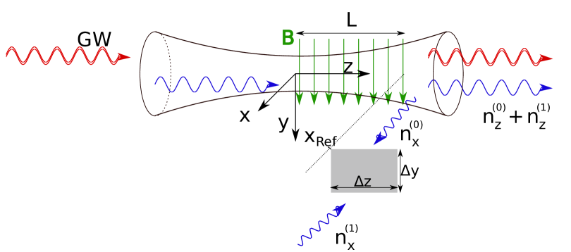
Figure 11: Illustration of the proposal [114] to exploit an EM GB to induce a GW-EMW conversion signal which is first order in $h_{c}$.

Depending on the overall sign of $\psi^{(1)}_{x}$, that is on $\delta$, this flux points either in the positive or negative $x$-direction. The idea is then to place at $x=\pm x_{\rm Ref}$ reflectors (e.g. fractal membranes) parallel to the $y$-$z$ plane, see Fig.  11, which could reflect and focus a portion of this flux to receivers and detectors placed at positions $x=\pm x_{\rm Det}$ with $x_{\rm Det}>x_{\rm Ref}$ which are further away from the GB and therefore expected to suffer less from noise [115]. The number of signal photons within a bandwidth $\Delta f_{0}$ around $f_{0}$ passing in a time interval $\Delta t$ through a detector surface element $\Delta S=\Delta y\Delta z$ in the $y$-$z$ plane, which extents from $y=0$ to $y=\Delta y$ in the $y$-direction and from $z=L$ to $z=L+\Delta z$ in the $z$-direction, is then

$$\Delta N_{x}^{(1)}(x_{\rm Det}) \simeq \frac{\eta}{4}\,h_{c}(f_{0})\,\left[\frac{\Delta f_{0}}{f_{0}}\right]B_{y}^{(0)}E_{0}L\,\Delta y\Delta z\,\Delta t\,\mathcal{F}^{(1)}_{x}(x_{\rm Ref})$$

$$= 3.15\,\eta\,\left[\frac{h_{c}(f_{0})}{10^{-23}}\right]\,\left[\frac{\frac{\Delta f_{0}}{f_{0}}}{10^{-6}}\right]\,\left[\frac{B_{y}^{(0)}}{\rm 1\,T}\right]\,\left[\frac{E_{0}}{\rm 5\times 10^{5}\,V/m}\right]\,\left[\frac{L}{\rm m}\right]\,\left[\frac{\Delta y\Delta z}{\rm 0.01\,m^{2}}\right]\,\left[\frac{\Delta t}{\rm s}\right]\,\left[\frac{\mathcal{F}^{(1)}_{x}(x_{\rm Ref})}{10^{-5}}\right]\,,$$

where $0<\eta<1$ is the reflectivity of the reflector and

$$\mathcal{F}^{(1)}_{x}(x) = \frac{1}{4\pi}\frac{w_{0}z_{R}}{\Delta y\Delta z}\,\int\limits_{0}^{2\pi}{\rm d}\delta\,\left|\int\limits_{0}^{\frac{\Delta y}{w_{0}}}{\rm d}y^{\prime}\,\int\limits_{\frac{L}{z_{R}}}^{\frac{L+\Delta z}{z_{R}}}{\rm d}z^{\prime}\,\psi^{(1)}_{x}\left(\frac{w_{0}}{z_{R}},x^{\prime},y^{\prime},z^{\prime},\delta\right)\right|\,.$$ (4.14)

Numerical results for $\mathcal{F}^{(1)}_{x}(x,w_{0})$, for particular values of $f_{0}$, $\Delta y$, $\Delta z$, and $L$, are displayed in Fig. 12 (top panels). Right to the red lines, the Gaussian beam amplitude has dropped by a factor more than $1/e$. We assume that placing the reflector in this region will cause only minor disturbances of the signal photon flux. Based on this assumption we find a benchmark value of $10^{-5}$ for $\mathcal{F}_{x}^{1}$ which we have taken in Eq. (4.2.2). As benchmarks for the amplitude $E_{0}$ and the relative bandwidth $\Delta f_{0}/f_{0}$ of the GB we have taken in Eq. (4.2.2) values which can be achieved with a state-of-the-art free-running high-power (MW scale) gyrotron in this frequency range [128, 129].

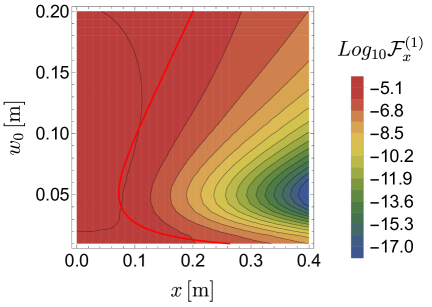
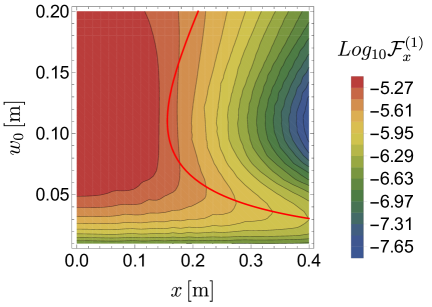
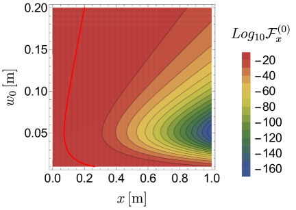
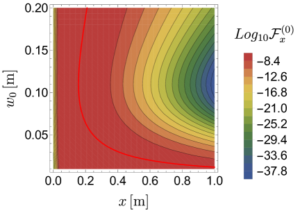
Figure 12: Contours of $\mathcal{F}_{x}^{(1)}$ (top panels) and $\mathcal{F}_{x}^{(0)}$ (bottom panels) in the $x$-$w_{0}$ plane, for $f_{0}=$40\text{\,}\mathrm{GHz}$$, $\Delta y=$0.1\text{\,}\mathrm{m}$$, $\Delta z=$0.1\text{\,}\mathrm{m}$$, and $L=$1\text{\,}\mathrm{m}$$ (left panels) and $L=$5\text{\,}\mathrm{m}$$ (right panels). The red lines indicate the distance in the $x$-direction for which $x=w(L+\Delta z)=w_{0}\sqrt{1+[{(L+\Delta z)}/{z_{R}}]^{2}}$.

The zeroth order flux in the $x$-direction propagates radially out from the GB’s axis,

$$n_{x}^{(0)} = \frac{\alpha_{p}}{4\pi}\frac{E_{0}^{2}}{f_{0}}\,\psi^{(0)}_{x}\left(\frac{w_{0}}{z_{R}},x^{\prime},y^{\prime},z^{\prime}\right)$$

$$= \frac{1.25\times 10^{31}}{{\rm m}^{2}\,{\rm s}}\,\alpha_{p}\,\left[\frac{f_{0}}{\rm 40\,GHz}\right]^{-1}\,\left[\frac{E_{0}}{\rm 5\times 10^{5}\,V/m}\right]^{2}\,\psi^{(0)}_{x}\left(\frac{w_{0}}{z_{R}},x^{\prime},y^{\prime},z^{\prime}\right)\,,$$

where $\alpha_{p}\ll 1$ is the ratio of the $y$ to $x$ components of the GB electric field and [118]

$$\psi^{(0)}_{x}\left(\frac{w_{0}}{z_{R}},x^{\prime},y^{\prime},z^{\prime}\right)=\frac{w_{0}}{z_{R}}\frac{\frac{x^{\prime}}{z^{\prime}}\exp\left(-2\frac{{x^{\prime}}^{2}+{y^{\prime}}^{2}}{\left[1+{z^{\prime}}^{2}\right]}\right)}{\left[1+{z^{\prime}}^{2}\right]\left[1+{z^{\prime}}^{-2}\right]}\,.$$ (4.16)

The corresponding number of background photons passing in a time interval $\Delta t$ through the detector surface is then

$$\Delta N_{x}^{(0)}(x_{\rm Det})\simeq 1.25\times 10^{-11}\,\alpha_{p}\,\left[\frac{f_{0}}{\rm 40\,GHz}\right]^{-1}\,\left[\frac{E_{0}}{\rm 5\times 10^{5}\,V/m}\right]^{2}\,\left[\frac{\Delta y\Delta z}{\rm 0.01\,m^{2}}\right]\,\left[\frac{\Delta t}{\rm s}\right]\,\left[\frac{\mathcal{F}^{(0)}_{x}(x_{\rm Det})}{10^{-40}}\right]\,,$$ (4.17)

with

$$\mathcal{F}^{(0)}_{x}(x) = \frac{w_{0}z_{R}}{\Delta y\Delta z}\,\int\limits_{0}^{\frac{\Delta y}{w_{0}}}{\rm d}y^{\prime}\,\int\limits_{\frac{L}{z_{R}}}^{\frac{L+\Delta z}{z_{R}}}{\rm d}z^{\prime}\,\psi^{(0)}_{x}\left(\frac{w_{0}}{z_{R}},x^{\prime},y^{\prime},z^{\prime}\right)\,.$$ (4.18)

Numerical results for $\mathcal{F}^{(0)}_{x}(x,w_{0})$, for particular values of $f_{0}$, $\Delta y$, $\Delta z$, and $L$, are displayed in Fig. 12 (bottom panels). As its benchmark we have taken in (4.17) a value of $10^{-40}$ which is appropriate when the detectors are put at $x_{\rm Det}=0.45\,{\rm m}$ or $1\,{\rm m}$, for $L=1\,{\rm m}$ or $5\,{\rm m}$, respectively, cf. Fig. 12 (bottom panels). Therefore, this direct background from the GB is expected to be quite small if the receiver is placed sufficiently away from the beam. Moreover, it should occur simultaneously at the two detectors located at $x=\pm x_{\rm Det}$, while the signal ($n_{x}^{(1)}$ propagating towards $x=0$, see Fig. 11), for fixed phase difference $\delta$, occurs only at one of the two detectors. Nevertheless, this consideration neglects the possibility that the radiation from the GB is perturbed by the presence of the reflectors which in turn could disturb the signal photon flux. Furthermore the reflectors can be a noise source if the GB interacts with them. This kind of noise can be minimized by placing the reflectors at least right to the red lines in Fig. 12 where the GB amplitude has fallen off by $1/e$ [120]. However, the exact noise level, which is introduced by the interaction of the GB with the reflectors, has to be evaluated in a future study. If all these sources can be dealt with and the apparatus can be designed in such a way that finally the dark count rate (4.8) in SPD is the dominating background, then the sensitivity is given by

$$\left[h^{\rm CGMB}_{c}\right]_{\rm sens}^{\rm GB} \simeq 4.02\times 10^{-29}\,\eta^{-1}\,\left[\frac{{\rm S}/{\rm N}}{2}\right]\,\left[\frac{\Delta t}{10^{4}\,s}\right]^{-1/2}\,\left[\frac{\frac{\Delta f_{0}}{f_{0}}}{10^{-6}}\right]^{-1}\times$$

$$\times\,\epsilon^{-1}\,\left[\frac{\Gamma_{\rm D}}{10^{-3}\,\text{Hz}}\right]^{1/2}\,\left[\frac{E_{0}}{\rm 5\times 10^{5}\,V/m}\right]^{-1}\,\left[\frac{B_{y}^{(0)}}{\rm 10\,T}\right]^{-1}\,\left[\frac{L}{\rm 5\,m}\right]^{-1}\,\left[\frac{\Delta y\Delta z}{\rm 0.01\,m^{2}}\right]^{-1}\,\left[\frac{\mathcal{F}_{x}^{(1)}(x_{\rm Ref})}{10^{-5}}\right]^{-1}.$$

Here we have taken current state-of-the-art benchmarks for the various experimental parameters.

This is still three orders of magnitude above the CGMB predictions with early time equilibration, corresponding to $T_{\rm max}>M_{P}$ and an approximate saturation of the dark radiation bound (3.5), cf. Fig. 10. However, the latter may be reached and eventually surpassed by progress in the development of gyrotrons, SPD, and magnets. In fact, one may gain an order of magnitude in $h_{c}$ sensitivity by increasing the total power of the gyrotron by two orders of magnitude to $\sim 100$ MW (and thus $E_{0}$ by one order of magnitude) and another order of magnitude in $h_{c}$ sensitivity by increasing the stable running time of the gyrotron by two orders of magnitude to $\Delta t\sim 10^{6}$ s. The remaining order of magnitude one may gain by developing SPD with a dark count rate of order $10^{-5}$ s. Further improvements can be obtained by increasing the reflector size and by developing magnets with higher magnetic field and length. A sensitivity corresponding to $T_{\rm max}=M_{P}$ seems to be reachable in the not-so-distant future. In case of the detection of a signal, one may explore the frequency region around the nominal frequency of the gyrotron in a range $\Delta f_{0}\sim 10^{-3}f_{0}=40\,{\rm MHz}\,[f_{0}/(40\,{\rm GHz})]$ by changing the acceleration voltage of the gyrotron.

5 Summary and outlook

Based on the pioneering work of Refs.  [8, 9], we have provided general formulae for the production rate of GWs from a primordial thermal plasma with sub-Planckian temperatures in an arbitrary theory with gauge fields, real scalars and Weyl fermions (cf. Sect. 2.1 and Appendix A) and derived general expressions for $\Omega_{\rm CGMB}(f)$, the current energy fraction of those GWs per logarithmic frequency interval (see Sect. 2.2). It is found to peak around $f_{\rm peak}^{\Omega_{\rm CGMB}}\simeq 80\,{\rm GHz}\,[106.75/g_{*s}(T_{\rm max})]^{1/3}$ (cf. Eqs. (2.42), (2.47) and Table 2) – hence we chose CGMB (for Cosmic Gravitational Microwave Background) as the acronym for this stochastic background. Its overall magnitude scales approximately linearly with the maximum temperature which the primordial plasma attained at the beginning of the standard hot big bang era (cf. Eq. (2.2)) while also depending on $g_{*s}(T_{\rm max})$. For weakly coupled theories, the peak emission satisfies the approximate scaling of Eq. (2.48), (see also Eqs. (2.43) and (2.44)) implying that for a given $T_{\rm max}$ the SM will typically maximize the CGMB with respect to its value in weakly coupled extensions. With the leading behaviour of the peak frequency and the magnitude of the CGMB being determined by $T_{\rm max}$ and $g_{*s}(T_{\rm max})$, the CGMB can therefore act as a hot big bang thermometer and, additionally, allow a measurement of the number of thermalized BSM degrees of freedom, $g_{*s}(T_{\rm max})-g_{*s,{\rm SM}}(T_{\rm max})$. As special cases, we have determined the CGMB spectrum for the cases of a SM (cf. Sect. 2.3), a $\nu$MSM, a SMASH (cf. Sect. 2.4), as well as an MSSM (cf. Sect. 2.5) plasma. We confirmed that the leading model dependence is indeed captured by the effects of $g_{*s}(T_{\rm max})$, so that within a broad class of weakly coupled SM extensions, a simple comparison of a hypothetical measurement of the CGMB peak with the SM prediction would allow to estimate $g^{1/3}_{*s}(T_{\rm max})$ and $T_{\rm max}$ in a model-independent manner and with respective theoretical accuracies that should be better than the MSSM results of 15% and 40% (e.g. $\sim 1\%$ and $5\%$ in SMASH).

The previous features of the CGMB apply for $T_{\rm max}<M_{P}$, while for larger early-time temperatures one expects gravitons to thermalize and lead to the blackbody spectrum of Eq. (2.49), with peak frequencies and maxima scaling with $g_{*s}(M_{P})$ as in Eqs. (2.28) and (2.50), and independent of the concrete value of $T_{\rm max}$ and of any additional model details. Here, a possible detection would allow a precise determination of $g_{*s}(T_{\rm max})$.

We have found that current dark radiation constraints from BBN and CMB on the total energy density fraction in GWs cannot yet probe the out-of-equilibrium gravitational wave emission with $T_{\rm max}<M_{P}$, as a naive application of the constraints implies a trans-Planckian upper bound on $T_{\rm max}$ around $10^{19}$ GeV, cf. Table 1. Nevertheless we find the intriguing result that the CGMB background with early time equilibration (i.e. with $T_{\rm max}>M_{P}$) just about saturates the dark radiation constraint of Eq. (3.5), to be compared with the prediction of Eq. (3.7). The former bound corresponds to homogeneous initial conditions for the gravitational waves, as appropriate under the assumption of thermal equilibrium at early times. Applying the bound of Eq. (3.5) and using the determination of $g_{*s,{\rm SM}}$ of Appendix B (illustrated in Fig. 3) would discard a CGMB with early time equilibration in models in which $g_{*s}$ is augmented by less than $\sim 4$ units.

Further improvements on the dark radiation constraints would discard early time equilibration of the gravitational waves in a large class of models, and start constraining the out-of-equilibrium CGMB for sub-Planckian $T_{\rm max}$. In case that future CMB constraints on dark radiation reach the theoretical uncertainty from the pure SM expectation ($\Delta N_{\rm eff}=0.001$), the upper bound of $T_{\rm max}$ can be improved to sub-Planckian values around $2\times 10^{17}$ GeV, cf. Table 1.

Further progress should come from direct detection of GWs. However, all the current upper bounds from direct searches for stochastic GWs and also the projected sensitivities of planned GW detectors are at least nine orders of magnitude away from the prediction of the maximally allowed characteristic amplitude $h_{c}$ of the CGMB respecting the dark radiation constraint (corresponding to the CGMB with early time equilibration), cf. Fig. 8.

Conversion of GWs into EMWs in a static magnetic field has been identified as a promising search technique for stochastic GWs at frequencies around $f_{\rm peak}^{h_{c}^{\rm CGMB}}\simeq 40\,{\rm GHz}\,[106.75/g_{*\rho}(T_{\rm max})]^{1/3}$, where the characteristic amplitude $h_{c}^{\rm CGMB}(f)$ of the CGMB attains its maximum, cf. Eq. (2.42) and Table 2. We investigated the prospects of GW-EMW conversion in state-of-the-art superconducting magnets used in present and near future axion experiments and the detection of the generated EMWs/photons with dedicated detectors appropriate around 40 GHz. The projected sensitivity of this technique, cf. Table 3 and Fig. 10, turned out to fail to beat the dark radiation constraint on $h_{c}^{\rm CGMB}$ by about six orders of magnitude. We then investigated the prospects of a proposal exploiting an additional EM Gaussian beam, delivered by a MW-scale 40 GHz gyrotron, propagating along the magnetic conversion region in order to generate a transverse EMW conversion signal which is first order in $h_{c}$. Assuming state-of-the-art benchmarks for the gyrotron, the detector performance and the magnetic field strength and length, the projected sensitivity in $h_{c}$ is still three orders of magnitude above the maximum amplitude of the equilibrated CGMB (see Eq. (2.50)) which saturates the dark radiation bound, cf. Fig. 10. However, the latter may be reached by progress in the development of gyrotrons towards higher power and stable run time, single photon detection towards lower dark count rate, and superconducting magnets towards higher magnetic fields. The direct detection of the CGMB at a level corresponding to $T_{\rm max}\sim M_{P}$ by such a magnetic conversion experiment seems possible, although challenging. In this connection, it should be emphasized that the search for the CGMB is truly a critical endeavour. Any measurement of $T_{\rm max}$ above $6.6\times 10^{15}\,{\rm GeV}$ would be ground-breaking, since it would rule out standard inflation as a viable pre hot big bang scenario.

It would be very interesting to investigate the CGMB also in other BSM models with a complete and consistent cosmological history and thus giving a prediction of $T_{\rm max}$, such as for example the model in Ref. [130]. Furthermore, it seems worthwhile to explore more deeply the possible synergies between axion and GW experiments which we have been touching upon in this paper.

Currently, a community is forming which seriously considers the search for high-frequency gravitational waves [102]. Detecting the CGMB sets an ambitious, but rewarding goal for this enterprise.

Appendix A Loop functions for the rate of GW production from the primordial plasma at full leading order

Here we collect formula for the loop functions $\eta_{gg}(\hat{k})$, $\eta_{sg}(\hat{k})$, $\eta_{fg}(\hat{k})$, $\eta_{sf}(\hat{k})$ appearing in Eq. (2.9). We use the results of Ref. [9] with a simplified notation. One can define a set of six integrals ${\cal I}_{\pm}(\hat{k}),{\cal J}_{\pm}(\hat{k}),{\cal K},{\cal L}$, in terms of which the above functions are expressed as:

$$\begin{aligned} \eta_{gg}(\hat{k})=&\,-4{\cal I}_{+}(\hat{k})-4{\cal J}_{+}(\hat{k}),\\ \eta_{sg}(\hat{k})=&\,-{\cal I}_{+}(\hat{k})-{\cal J}_{+}(\hat{k})=\frac{1}{4}\eta_{gg}(\hat{k}),\\ \eta_{sf}(\hat{k})=&\,4{\cal K}(\hat{k})+2{\cal L}(\hat{k}),\\ \eta_{fg}(\hat{k})=&\,4{\cal I}_{-}(\hat{k})+4{\cal J}_{-}(\hat{k}).\end{aligned}$$ (A.1)

The loop integrals are given next:

In the above expressions, one has

$$n_{b}(x)=\frac{1}{e^{x}-1},$$ (A.2)

while the functions $L_{i}^{\pm}(x,y),M_{i}^{\pm}(x,y)$, with $i=1,2,3$ are defined below:

$$\begin{aligned} L_{1}^{\pm}(x,y)=&\,\log\left(\frac{1\mp e^{-\frac{1}{2}(x+y)}}{1\mp e^{\frac{1}{2}(x-y)}}\right),\\ L_{2}^{\pm}(x,y)=&\,{\rm Li}_{2}(\pm e^{\frac{1}{2}(x-y)})-{\rm Li}_{2}(\pm e^{-\frac{1}{2}(x+y)}),\\ L_{3}^{\pm}(x,y)=&\,{\rm Li}_{3}(\pm e^{\frac{1}{2}(x-y)})-{\rm Li}_{3}(\pm e^{-\frac{1}{2}(x+y)}),\\ M_{1}^{\pm}(x,y)=&\,\log\left(\frac{1\mp e^{-\frac{1}{2}(x-y)}}{1\mp e^{-\frac{1}{2}(x+y)}}\right),\\ M_{2}^{\pm}(x,y)=&\,{\rm Li}_{2}(\pm e^{-\frac{1}{2}(x+y)})+{\rm Li}_{2}(\pm e^{-\frac{1}{2}(x-y)}),\\ M_{3}^{\pm}(x,y)=&\,{\rm Li}_{3}(\pm e^{-\frac{1}{2}(x+y)})-{\rm Li}_{3}(\pm e^{-\frac{1}{2}(x-y)}).\end{aligned}$$ (A.3)

As explained in the main text, the integrals above include a subtraction of infrared divergences, so that they remain finite. The subtraction corresponds to the last term in the integrand of ${\cal I}_{\pm}(\hat{k})$.

Appendix B Effective number of degrees of freedom of the SM, the $\nu$MSM and the SMASH plasma

In the primordial plasma, the thermal contributions to the effective potential correspond to the free-energy density. Thermodynamic relations imply that the latter is equal to minus the plasma’s pressure $p$:

$$p(\phi_{i})=-\left[V_{\rm eff}(\phi_{i},T)-V_{\rm eff}(\phi_{i},0)\right].$$ (B.1)

In the equation above, $\phi_{i}$ denote the scalar field backgrounds, and the subtraction of the second term above guarantees that the pressure is zero in the vacuum ($T=0$). We will assume that the system relaxes to the minimum of the effective potential, so that we will evaluate the backgrounds at the configurations $\phi_{i}=\bar{\phi}_{i}$ that extremize $V_{\rm eff}$:

$$\left.\frac{\partial V_{\rm eff}(\phi_{i},T)}{\partial\phi_{j}}\right|_{\phi_{i}=\bar{\phi}_{i}(T)}=0.$$ (B.2)

The effective potential with its finite-temperature correction at one-loop plus higher-order QCD effects can be written as:

$$V_{\rm eff}(\phi_{i},T)=V(\phi_{i})+V^{\rm CW}(\phi_{i},T)+V^{T}(\phi_{i},T)+V^{\rm QCD}(T).$$ (B.3)

Above, $V$ is the tree-level potential, $V^{\rm CW}$ the usual one-loop Coleman-Weinberg contribution at zero temperature, $V^{T}$ the one-loop thermal correction to the potential, and $V^{\rm QCD}$ includes two and three-loop thermal corrections induced by QCD effects, which are known for zero field backgrounds. Note that we have included a temperature-dependence in the Coleman-Weinberg vacuum piece. The reason is that achieving accuracy in the finite-temperature effects near a phase transition requires a resummation of thermal contributions to the 2 point functions – daisy resummation – which can be implemented by replacing the effective masses in the vacuum propagators by temperature corrected masses; this explains the $T$ dependence in the Coleman-Weinberg piece. The daisy resummation is usually performed by keeping the leading terms of the corrections to the two point functions in a high-temperature expansion. However, as noted in Ref. [36], achieving accuracy across a phase transition, i.e. for temperatures below the masses gained by particles during the transition, requires to go beyond the high-$T$ expansion. As we consider temperatures above the SM’s electroweak crossover, for the SM and $\nu$MSM we use a traditional daisy resummation. For SMASH, for which the PQ phase transition lies much above the electroweak scale, we implement the improved resummation of Ref. [36] for the corrections involving fields that acquire masses during the PQ transition.

In the Landau gauge and in the $\overline{\rm MS}$ scheme, $V^{\rm CW}(\phi_{i},T)$ and $V^{T}(\phi_{i},T)$ are given by

$$\begin{aligned} V^{\rm CW}(\phi_{i},T)=&\,\frac{1}{64\pi^{2}}\left[\sum_{V}m^{4}_{V}(\phi_{i},T)\left(\log\frac{m^{2}_{V}(\phi_{i},T)}{\mu^{2}}-\frac{5}{6}\right)+\sum_{S}m^{4}_{S}(\phi_{i},T)\left(\log\frac{m^{2}_{S}(\phi_{i},T)}{\mu^{2}}-\frac{3}{2}\right)\right.\\ &\left.-\sum_{F}m^{4}_{F}(\phi_{i},T)\left(\log\frac{m^{2}_{F}(\phi_{i},T)}{\mu^{2}}-\frac{3}{2}\right)\right],\\ V^{T}=&\,\frac{T^{4}}{2\pi^{2}}\left[\sum_{B}J_{B}\left(\frac{m^{2}_{B}(\phi_{i},T)}{T^{2}}\right)-\sum_{F}J_{F}\left(\frac{m^{2}_{F}(\phi_{i},T)}{T^{2}}\right)-\sum_{G}J_{B}\left(0\right)\right].\end{aligned}$$ (B.4)

In the previous formulae, $V,S,F$ and $G$ correspond to massive gauge bosons, real scalars, Weyl fermions and ghosts. It is assumed that for gauge bosons one has to sum over the three polarizations that propagate in the Landau gauge, while for fermions one has to sum over two helicities, and for ghosts one should count one degree of freedom per generator of each gauge group. $m^{2}_{V/S/F}(\phi_{i},T)$ are the field-dependent masses in the background of $\phi_{i}$, including the thermal corrections from the (improved) daisy resummation. $\mu$ is the renormalization scale, while the thermal loop functions $J_{B}$ and $J_{F}$ are

$$\begin{aligned} J_{B}(x)=\int_{0}^{\infty}dy\,y^{2}\log\left[1-\exp(-\sqrt{x+y^{2}})\right],\\ J_{F}(x)=\int_{0}^{\infty}dy\,y^{2}\log\left[1+\exp(-\sqrt{x+y^{2}})\right].\end{aligned}$$ (B.5)

The last missing piece in the effective potential in Eq. (B.3) corresponds to higher loop QCD contributions, which have been computed in Ref. [29] up to three-loop order in a theory with arbitrary massless QCD flavours. This allows to apply the QCD corrections for all the models of interest.

Once the pressure is calculated from the minimization of the effective potential that follows from the above equations, the energy density $\rho$, standard thermodynamic relations allow to compute the entropy density $s$ and the specific heat capacity $c=1/V(\partial U/\partial T)|_{V}$ as

$$\rho= \,T\frac{\partial p}{\partial T}-p, s= \,\frac{\partial p}{\partial T}, c= \,T\,\frac{\partial^{2}p}{\partial T^{2}}.$$ (B.6)

From the former quantities one defines the effective numbers of degrees of freedom $g_{*\rho}$, $g_{*s}$, $g_{*c}$ by writing

$$\rho= \,\frac{\pi^{2}}{30}\,g_{*\rho}(T)T^{4}, s= \,\frac{2\pi^{2}}{45}\,g_{*s}(T)T^{3}, c= \,\frac{2\pi^{2}}{15}\,g_{*c}(T)T^{3}$$ (B.7)

In our calculations of the effective potential, we use a renormalization scale proportional to the temperature, $\mu=\kappa 2\pi T$ with $\kappa\in\{1/2,1,2\}$. It should be noted that for the SM our perturbative calculations are not trustworthy for temperatures below the electroweak crossover, as the daisy resummation does not capture the decoupling of the degrees of freedom acquiring masses during the crossover. Furthermore, for lower temperatures the QCD interactions become nonperturbative, and other techniques are necessary [20, 21]. In this paper we neglect the gravitational wave production at temperatures below the electroweak crossover.

For SMASH we introduce an additional correction coming from the loss of chemical equilibrium of the axion, which implies a separate conservation of the entropy of the axion and the rest of the thermal bath, and thus separate temperatures for both, to be denoted as $T_{\rm axion}$ and $T$. Labeling the results for $g^{\rm SMASH}_{*\rho}$, $g^{\rm SMASH}_{*s}$, $g^{\rm SMASH}_{*c}$ under the assumption of chemical equilibrium for the axion with the superfix “eq”, the quantities accounting for decoupling can be written as [36]

$$\begin{aligned} g^{\rm SMASH}_{*\rho}=&\,g^{\rm SMASH,eq}_{*\rho}-1+\left(\frac{T_{\rm axion}}{T}\right)^{4},&g^{\rm SMASH}_{*s}=&\,g^{\rm SMASH,eq}_{*s}-1+\left(\frac{T_{\rm axion}}{T}\right)^{3},\\ g^{\rm SMASH}_{*c}=&\,g^{\rm SMASH,eq}_{*c}-1+\left(\frac{T_{\rm axion}}{T}\right)^{3}.\end{aligned}$$ (B.8)

Appendix C Upper bound on $T_{\rm max}$ in inflationary cosmology

The hypothesis of inflation postulates a period of accelerated expansion, $\ddot{a}>0$, in the very early universe [131, 132], preceding the standard radiation-dominated era. It offers a physical model for the origin of the initial conditions of hot big bang cosmology. In slow-roll inflationary cosmology [133, 134], the energy scale at the end of inflation, $\rho_{\rm inf}$, can be inferred from the amplitude $A_{S}$ of scalar perturbations generated during inflation and the tensor-to-scalar ratio $r$ via

$$\rho_{\rm inf}\equiv 3H_{\rm inf}^{2}M_{P}^{2}\approx\frac{3}{2}\,\pi^{2}\,r\,A_{S}M_{P}^{4}\,,$$ (C.1)

where $H_{\rm inf}$ is the Hubble expansion rate during inflation. The upper limit on $r$ obtained from CMB observations of the BICEP2/Keck Array and Planck Collaborations provides an upper bound on $\rho_{\rm inf}$ [52],

$$\rho_{\rm inf}\,<\,\left(1.6\times 10^{16}\,{\rm GeV}\right)^{4}\hskip 12.91663pt(95\%\ {\rm CL})\,.$$ (C.2)

This may be turned into an upper bound on the maximum temperature of the post-inflationary universe by assuming instantaneous and thus maximally efficient reheating to a radiation dominated universe with energy density

$$\frac{\pi^{2}}{30}g_{*\rho}(T_{\rm max}^{\rm up})T^{\rm up\,4}_{\rm max}=\rho_{\rm inf}\,,$$ (C.3)

which in combination with (C.2) leads to

$$T^{\rm up}_{\rm max}=\left[\frac{\rho_{\rm inf}}{\frac{\pi^{2}}{30}\,g_{*\rho}(T_{\rm max}^{\rm up})}\right]^{1/4}<6.6\times 10^{15}\,{\rm GeV}\left[\frac{106.75}{g_{*\rho}(T_{\rm max}^{\rm up})}\right]^{1/4}\,.$$ (C.4)

In SMASH [14], $g_{*\rho}(10^{15}\,{\rm GeV})\simeq 124.5$.

Appendix D 3D effects in GW-EMW conversion experiments

D.1 Waveguide effect

If the magnetic conversion volume is surrounded by a waveguide the phase velocity inside the waveguide will be different from the speed of light. We illustrate this for a circular waveguide which is infinite in $z$-direction and has radius $a$. For TE modes we have $E_{z}=0$ everywhere and the normal derivative of $B_{z}$ vanishes at the boundaries. After the application of all boundary conditions we obtain for the longitudinal $B$-field:

$$B_{z}=F\sin\left(\nu(\phi-\phi_{0})\right)J_{\nu}(k_{c}r)e^{-ik_{z}z}\,,$$ (D.1)

where $F,\phi_{0}$ are constants, $\nu$ is an integer, $r,\phi$ and $z$ are the three coordinates in the cylindrical coordinate system, $J_{\nu}$ is the Bessel function of the first kind and $k_{c}=\frac{p_{\nu n}}{a}$ is the transversal momentum, where $p_{\nu n}$ is the $n$th zero of $J_{\nu}^{\prime}(x)$. The total wave vector is given by $k^{2}=k_{c}^{2}+k_{z}^{2}={\omega^{2}}$. From the longitudinal field $B_{z}$ we can derive all other electromagnetic fields in the cylindrical waveguide. The phase velocity is:

$$v_{p}=\frac{\omega}{k_{z}}=\frac{\omega}{\sqrt{{\omega^{2}}{}-\left(\frac{p_{\nu n}}{a}\right)^{2}}}=\frac{1}{\sqrt{1-\left(\frac{p_{\nu n}}{a\omega}\right)^{2}}}.$$ (D.2)

If the radius of the waveguide is much larger than the wavelength we can expand the square root and get:

$$v_{p}\approx 1+\frac{1}{2}\left(\frac{p_{\nu n}\lambda}{2\pi a}\right)^{2}\,.$$ (D.3)

Therefore the phase velocity is larger than the speed of light.

For a coherent and thus efficient conversion of gravitons into photons inside a waveguide, they should be in phase all along the waveguide. Therefore the phase difference between gravitons and photons has to be smaller than $\pi$ at the end of the waveguide:

$$k_{G}L-k_{z}L\ll\pi,$$ (D.4)

where $k_{G}=\omega$ is the graviton dispersion, $k_{z}$ is the photon wave vector in $z$-direction and $L$ the length of the external $B$-field. Plugging equation (D.3) into equation (D.4) yields the condition:

$$L\ll\left(\frac{2\pi}{p_{\nu n}}\right)^{2}\frac{a^{2}}{\lambda}.$$ (D.5)

For the dominating $TE_{11}$ mode we find $p_{11}=1.8$ and therefore in this case the prefactor is $\left(\frac{2\pi}{p_{\nu n}}\right)^{2}\approx 12$.

D.2 Diffraction in open systems

If no waveguide encloses the magnetized region we only have to take into account diffraction effects. For a magnetized region of length $L$ along the $z$-direction with a circular shape in the $xy$-plane we obtain the diffraction angel $\theta$ in the far field as:

$$\tan\theta=1.22\frac{\lambda}{d},$$ (D.6)

where $d$ is the diameter of the magnetized region. For IAXO we get $\theta=0.6^{\circ}$ and therefore diffraction is negligible. In the case of ALPS IIc the diffraction angle is much larger and due to the huge length of ALPS IIc it cannot be neglected.

References

- [1] M. Kawasaki, K. Kohri and N. Sugiyama, “Cosmological constraints on late time entropy production,” Phys. Rev. Lett. 82 (1999), 4168 [arXiv:astro-ph/9811437 [astro-ph]].
- [2] M. Kawasaki, K. Kohri and N. Sugiyama, “MeV scale reheating temperature and thermalization of neutrino background,” Phys. Rev. D 62 (2000), 023506 [arXiv:astro-ph/0002127 [astro-ph]].
- [3] G. F. Giudice, E. W. Kolb and A. Riotto, “Largest temperature of the radiation era and its cosmological implications,” Phys. Rev. D 64 (2001), 023508 [arXiv:hep-ph/0005123 [hep-ph]].
- [4] S. Hannestad, “What is the lowest possible reheating temperature?,” Phys. Rev. D 70 (2004), 043506 [arXiv:astro-ph/0403291 [astro-ph]].
- [5] T. Hasegawa, N. Hiroshima, K. Kohri, R. S. L. Hansen, T. Tram and S. Hannestad, “MeV-scale reheating temperature and thermalization of oscillating neutrinos by radiative and hadronic decays of massive particles,” JCAP 12 (2019), 012 [arXiv:1908.10189 [hep-ph]].
- [6] A. Sakharov, “Maximum temperature of thermal radiation,” Pisma Zh. Eksp. Teor. Fiz. 3 (1966) no.11, 439-441
- [7] E. W. Kolb and M. S. Turner, “The Early Universe,” Front. Phys. 69 (1990), 1-547
- [8] J. Ghiglieri and M. Laine, “Gravitational wave background from Standard Model physics: Qualitative features,” JCAP 1507 (2015) 022 [arXiv:1504.02569 [hep-ph]].
- [9] J. Ghiglieri, G. Jackson, M. Laine and Y. Zhu, “Gravitational wave background from Standard Model physics: Complete leading order,” JHEP 07 (2020), 092 [arXiv:2004.11392 [hep-ph]].
- [10] B. X. Hu and A. Loeb, “An Upper Limit on the Initial Temperature of the Radiation-Dominated Universe,” [arXiv:2004.02895 [astro-ph.CO]].
- [11] T. Asaka, S. Blanchet and M. Shaposhnikov, “The nuMSM, dark matter and neutrino masses,” Phys. Lett. B 631 (2005) 151 [hep-ph/0503065].
- [12] T. Asaka and M. Shaposhnikov, “The nuMSM, dark matter and baryon asymmetry of the Universe,” Phys. Lett. B 620 (2005) 17 [hep-ph/0505013].
- [13] G. Ballesteros, J. Redondo, A. Ringwald and C. Tamarit, “Unifying inflation with the axion, dark matter, baryogenesis and the seesaw mechanism,” Phys. Rev. Lett. 118 (2017) no.7, 071802 [arXiv:1608.05414 [hep-ph]].
- [14] G. Ballesteros, J. Redondo, A. Ringwald and C. Tamarit, “Standard Model–axion–seesaw–Higgs portal inflation. Five problems of particle physics and cosmology solved in one stroke,” JCAP 1708 (2017) 001 [arXiv:1610.01639 [hep-ph]].
- [15] P. Fayet, “Spontaneously Broken Supersymmetric Theories of Weak, Electromagnetic and Strong Interactions,” Phys. Lett. B 69 (1977), 489
- [16] G. R. Farrar and P. Fayet, “Phenomenology of the Production, Decay, and Detection of New Hadronic States Associated with Supersymmetry,” Phys. Lett. B 76 (1978), 575-579
- [17] H. Baer and X. Tata, “Weak scale supersymmetry: From superfields to scattering events,” Cambridge University Press, 2012.
- [18] P. B. Arnold, G. D. Moore and L. G. Yaffe, “Transport coefficients in high temperature gauge theories. 1. Leading log results,” JHEP 11 (2000), 001 [arXiv:hep-ph/0010177 [hep-ph]].
- [19] E. Braaten and R. D. Pisarski, “Soft Amplitudes in Hot Gauge Theories: A General Analysis,” Nucl. Phys. B 337 (1990), 569-634
- [20] M. Laine and M. Meyer, “Standard Model thermodynamics across the electroweak crossover,” JCAP 07 (2015), 035 [arXiv:1503.04935 [hep-ph]].
- [21] K. Saikawa and S. Shirai, “Primordial gravitational waves, precisely: The role of thermodynamics in the Standard Model,” JCAP 05 (2018), 035 [arXiv:1803.01038 [hep-ph]].
- [22] C. Caprini and D. G. Figueroa, “Cosmological Backgrounds of Gravitational Waves,” Class. Quant. Grav. 35 (2018) no.16, 163001 [arXiv:1801.04268 [astro-ph.CO]].
- [23] M. x. Luo and Y. Xiao, “Two loop renormalization group equations in the standard model,” Phys. Rev. Lett. 90 (2003), 011601 [arXiv:hep-ph/0207271 [hep-ph]].
- [24] A. G. M. Pickering, J. A. Gracey and D. R. T. Jones, “Three loop gauge beta function for the most general single gauge coupling theory,” Phys. Lett. B 510 (2001), 347-354 [erratum: Phys. Lett. B 535 (2002), 377] [arXiv:hep-ph/0104247 [hep-ph]].
- [25] R. Hempfling and B. A. Kniehl, “On the relation between the fermion pole mass and MS Yukawa coupling in the standard model,” Phys. Rev. D 51 (1995), 1386-1394 [arXiv:hep-ph/9408313 [hep-ph]].
- [26] K. G. Chetyrkin and M. Steinhauser, “The Relation between the MS-bar and the on-shell quark mass at order alpha(s)**3,” Nucl. Phys. B 573 (2000), 617-651 [arXiv:hep-ph/9911434 [hep-ph]].
- [27] K. Melnikov and T. v. Ritbergen, “The Three loop relation between the MS-bar and the pole quark masses,” Phys. Lett. B 482 (2000), 99-108 [arXiv:hep-ph/9912391 [hep-ph]].
- [28] G. Degrassi, S. Di Vita, J. Elias-Miro, J. R. Espinosa, G. F. Giudice, G. Isidori and A. Strumia, “Higgs mass and vacuum stability in the Standard Model at NNLO,” JHEP 08 (2012), 098 [arXiv:1205.6497 [hep-ph]].
- [29] K. Kajantie, M. Laine, K. Rummukainen and Y. Schroder, “The Pressure of hot QCD up to ,” Phys. Rev. D 67 (2003) 105008 [hep-ph/0211321].
- [30] S. Phinney et al., “The Big Bang Observer: Direct detection of gravitational waves from the birth of the Universe to the Present,” NASA Mission Concept Study (2004).
- [31] B. P. Abbott et al. [LIGO Scientific], “Exploring the Sensitivity of Next Generation Gravitational Wave Detectors,” Class. Quant. Grav. 34 (2017) no.4, 044001 [arXiv:1607.08697 [astro-ph.IM]].
- [32] N. Seto, S. Kawamura and T. Nakamura, “Possibility of direct measurement of the acceleration of the universe using 0.1-Hz band laser interferometer gravitational wave antenna in space,” Phys. Rev. Lett. 87 (2001) 221103 [astro-ph/0108011].
- [33] M. Punturo et al., “The Einstein Telescope: A third-generation gravitational wave observatory,” Class. Quant. Grav. 27 (2010), 194002.
- [34] P. Amaro-Seoane et al. [LISA], “Laser Interferometer Space Antenna,” [arXiv:1702.00786 [astro-ph.IM]].
- [35] K. Schmitz, “New Sensitivity Curves for Gravitational-Wave Experiments” [Data set], Zenodo, [http://doi.org/10.5281/zenodo.3689582].
- [36] A. Ringwald, K. Saikawa and C. Tamarit, “Primordial gravitational waves in a minimal model of particle physics and cosmology,” [arXiv:2009.02050 [hep-ph]].
- [37] S. Kuroyanagi, K. Nakayama and J. Yokoyama, “Prospects of determination of reheating temperature after inflation by DECIGO,” PTEP 2015 (2015) no.1, 013E02 [arXiv:1410.6618 [astro-ph.CO]].
- [38] P. Minkowski, “ at a Rate of One Out of Muon Decays?,” Phys. Lett. B 67 (1977) 421.
- [39] M. Gell-Mann, P. Ramond and R. Slansky, “Complex Spinors and Unified Theories,” Conf. Proc. C 790927 (1979) 315 [arXiv:1306.4669 [hep-th]].
- [40] T. Yanagida, “Horizontal Symmetry And Masses Of Neutrinos,” Conf. Proc. C 7902131 (1979) 95 [Conf. Proc. C 7902131 (1979) 95].
- [41] R. N. Mohapatra and G. Senjanovic, “Neutrino Mass and Spontaneous Parity Violation,” Phys. Rev. Lett. 44 (1980) 912.
- [42] E. K. Akhmedov, V. A. Rubakov and A. Y. Smirnov, “Baryogenesis via neutrino oscillations,” Phys. Rev. Lett. 81 (1998) 1359 [hep-ph/9803255].
- [43] F. L. Bezrukov and M. Shaposhnikov, “The Standard Model Higgs boson as the inflaton,” Phys. Lett. B 659 (2008) 703 [arXiv:0710.3755 [hep-th]].
- [44] F. Bezrukov, D. Gorbunov and M. Shaposhnikov, “On initial conditions for the Hot Big Bang,” JCAP 06 (2009), 029 [arXiv:0812.3622 [hep-ph]].
- [45] Y. Hamada, H. Kawai, K. y. Oda and S. C. Park, “Higgs Inflation is Still Alive after the Results from BICEP2,” Phys. Rev. Lett. 112 (2014) no.24, 241301 [arXiv:1403.5043 [hep-ph]].
- [46] F. Bezrukov and M. Shaposhnikov, “Higgs inflation at the critical point,” Phys. Lett. B 734 (2014), 249-254 [arXiv:1403.6078 [hep-ph]].
- [47] J. L. F. Barbon and J. R. Espinosa, “On the Naturalness of Higgs Inflation,” Phys. Rev. D 79 (2009), 081302 [arXiv:0903.0355 [hep-ph]].
- [48] C. P. Burgess, H. M. Lee and M. Trott, “Power-counting and the Validity of the Classical Approximation During Inflation,” JHEP 09 (2009), 103 [arXiv:0902.4465 [hep-ph]].
- [49] F. Bezrukov, A. Magnin, M. Shaposhnikov and S. Sibiryakov, “Higgs inflation: consistency and generalisations,” JHEP 01 (2011), 016 [arXiv:1008.5157 [hep-ph]].
- [50] D. Gorbunov and A. Tokareva, “Scalaron the healer: removing the strong-coupling in the Higgs- and Higgs-dilaton inflations,” Phys. Lett. B 788 (2019), 37-41 [arXiv:1807.02392 [hep-ph]].
- [51] Y. Ema, “Dynamical Emergence of Scalaron in Higgs Inflation,” JCAP 09 (2019), 027 [arXiv:1907.00993 [hep-ph]].
- [52] Y. Akrami et al. [Planck Collaboration], “Planck 2018 results. X. Constraints on inflation,” arXiv:1807.06211 [astro-ph.CO].
- [53] R. D. Peccei and H. R. Quinn, “CP Conservation in the Presence of Instantons,” Phys. Rev. Lett. 38 (1977) 1440.
- [54] J. Preskill, M. B. Wise and F. Wilczek, “Cosmology of the Invisible Axion,” Phys. Lett. B 120 (1983) 127.
- [55] L. F. Abbott and P. Sikivie, “A Cosmological Bound on the Invisible Axion,” Phys. Lett. B 120 (1983) 133.
- [56] M. Dine and W. Fischler, “The Not So Harmless Axion,” Phys. Lett. B 120 (1983) 137.
- [57] S. Weinberg, “A New Light Boson?,” Phys. Rev. Lett. 40 (1978) 223.
- [58] F. Wilczek, “Problem of Strong p and t Invariance in the Presence of Instantons,” Phys. Rev. Lett. 40 (1978) 279.
- [59] E. Armengaud et al. [IAXO], “Physics potential of the International Axion Observatory (IAXO),” JCAP 06 (2019), 047 doi:10.1088/1475-7516/2019/06/047 [arXiv:1904.09155 [hep-ph]].
- [60] M. Fukugita and T. Yanagida, “Baryogenesis Without Grand Unification,” Phys. Lett. B 174 (1986) 45.
- [61] G. Ballesteros and J. A. Casas, “Large tensor-to-scalar ratio and running of the scalar spectral index with Instep Inflation,” Phys. Rev. D 91 (2015), 043502 [arXiv:1406.3342 [astro-ph.CO]].
- [62] A. Ito, J. Soda and M. Yamaguchi, “Analytic formula for the dynamics around inflation end and implications on primordial gravitational waves,” [arXiv:2009.03611 [astro-ph.CO]].
- [63] D. R. T. Jones, “Asymptotic Behavior of Supersymmetric Yang-Mills Theories in the Two Loop Approximation,” Nucl. Phys. B 87 (1975), 127
- [64] D. R. T. Jones and L. Mezincescu, “The Beta Function in Supersymmetric {Yang-Mills} Theory,” Phys. Lett. B 136 (1984), 242-244
- [65] P. C. West, “The Yukawa beta Function in N=1 Rigid Supersymmetric Theories,” Phys. Lett. B 137 (1984), 371-373
- [66] B. D. Fields, K. A. Olive, T. H. Yeh and C. Young, “Big-Bang Nucleosynthesis After Planck,” JCAP 03 (2020), 010 [arXiv:1912.01132 [astro-ph.CO]].
- [67] T. L. Smith, E. Pierpaoli and M. Kamionkowski, “A new cosmic microwave background constraint to primordial gravitational waves,” Phys. Rev. Lett. 97 (2006) 021301 [astro-ph/0603144].
- [68] I. Sendra and T. L. Smith, “Improved limits on short-wavelength gravitational waves from the cosmic microwave background,” Phys. Rev. D 85 (2012) 123002 [arXiv:1203.4232 [astro-ph.CO]].
- [69] L. Pagano, L. Salvati and A. Melchiorri, “New constraints on primordial gravitational waves from Planck 2015,” Phys. Lett. B 760 (2016) 823 [arXiv:1508.02393 [astro-ph.CO]].
- [70] T. J. Clarke, E. J. Copeland and A. Moss, “Constraints on primordial gravitational waves from the Cosmic Microwave Background,” JCAP 10 (2020), 002 [arXiv:2004.11396 [astro-ph.CO]].
- [71] J. J. Bennett, G. Buldgen, M. Drewes and Y. Y. Y. Wong, “Towards a precision calculation of the effective number of neutrinos in the Standard Model I: The QED equation of state,” JCAP 03 (2020), 003 [arXiv:1911.04504 [hep-ph]].
- [72] M. Escudero Abenza, “Precision early universe thermodynamics made simple: and neutrino decoupling in the Standard Model and beyond,” JCAP 05 (2020), 048 doi:10.1088/1475-7516/2020/05/048 [arXiv:2001.04466 [hep-ph]].
- [73] K. Akita and M. Yamaguchi, “A precision calculation of relic neutrino decoupling,” JCAP 08 (2020), 012 [arXiv:2005.07047 [hep-ph]].
- [74] J. Froustey, C. Pitrou and M. C. Volpe, “Neutrino decoupling including flavour oscillations and primordial nucleosynthesis,” [arXiv:2008.01074 [hep-ph]].
- [75] M. Gertsenshtein, “Wave resonance of light and gravitational waves,” Sov. Phys. JETP 14 (1962) 84.
- [76] D. Boccaletti, “Conversion of photons into gravitons and vice versa in a static electromagnetic field,” Nuovo Cimento 70 B (1970) 129.
- [77] Y. B. Zeldovich, “Electromagnetic and gravitational waves in a stationary magnetic field,” Sov. Phys. JETP 65 (1973) 1311.
- [78] W. K. De Logi and A. R. Mickelson, “Electrogravitational Conversion Cross-Sections in Static Electromagnetic Fields,” Phys. Rev. D 16 (1977) 2915.
- [79] G. Raffelt and L. Stodolsky, “Mixing of the Photon with Low Mass Particles,” Phys. Rev. D 37 (1988), 1237
- [80] V. Domcke and C. Garcia-Cely, “The CMB Rayleigh-Jeans tail as a detector of high-frequency gravitational waves,” [arXiv:2006.01161 [astro-ph.CO]].
- [81] K. L. Dooley et al., “GEO 600 and the GEO-HF upgrade program: successes and challenges,” Class. Quant. Grav. 33 (2016) 075009 [arXiv:1510.00317 [physics.ins-det]].
- [82] K. Somiya [KAGRA Collaboration], “Detector configuration of KAGRA: The Japanese cryogenic gravitational-wave detector,” Class. Quant. Grav. 29 (2012) 124007 [arXiv:1111.7185 [gr-qc]].
- [83] B. P. Abbott et al., “Sensitivity of the Advanced LIGO detectors at the beginning of gravitational wave astronomy,” Phys. Rev. D 93 (2016) no.11, 112004 Addendum: [Phys. Rev. D 97 (2018) no.5, 059901] [arXiv:1604.00439 [astro-ph.IM]].
- [84] F. Acernese et al. [VIRGO Collaboration], “Advanced Virgo: a second-generation interferometric gravitational wave detector,” Class. Quant. Grav. 32 (2015) no.2, 024001 [arXiv:1408.3978 [gr-qc]].
- [85] A. M. Cruise and R. M. J. Ingley, “A prototype gravitational wave detector for 100-MHz,” Class. Quant. Grav. 23 (2006) 6185.
- [86] A. Nishizawa et al., “Laser-interferometric Detectors for Gravitational Wave Background at 100 MHz: Detector Design and Sensitivity,” Phys. Rev. D 77 (2008) 022002 [arXiv:0710.1944 [gr-qc]].
- [87] T. Akutsu et al., “Search for a stochastic background of 100-MHz gravitational waves with laser interferometers,” Phys. Rev. Lett. 101 (2008) 101101 [arXiv:0803.4094 [gr-qc]].
- [88] A. S. Chou et al. [Holometer Collaboration], “MHz Gravitational Wave Constraints with Decameter Michelson Interferometers,” Phys. Rev. D 95 (2017) no.6, 063002 [arXiv:1611.05560 [astro-ph.IM]].
- [89] A. Ito, T. Ikeda, K. Miuchi and J. Soda, “Probing GHz Gravitational Waves with Graviton-magnon Resonance,” Eur. Phys. J. C 80 (2020) no.3, 179 [arXiv:1903.04843 [gr-qc]].
- [90] A. Ito and J. Soda, “A formalism for magnon gravitational wave detectors,” Eur. Phys. J. C 80 (2020) no.6, 545 [arXiv:2004.04646 [gr-qc]].
- [91] R. Barbieri, M. Cerdonio, G. Fiorentini and S. Vitale, “Axion To Magnon Conversion: A Scheme For The Detection Of Galactic Axions,” Phys. Lett. B 226 (1989) 357.
- [92] N. Crescini et al., “Operation of a ferromagnetic axion haloscope at eV,” Eur. Phys. J. C 78 (2018) no.9, 703 Erratum: [Eur. Phys. J. C 78 (2018) no.9, 813] [arXiv:1806.00310 [hep-ex]].
- [93] G. Flower, J. Bourhill, M. Goryachev and M. E. Tobar, “Broadening frequency range of a ferromagnetic axion haloscope with strongly coupled cavity–magnon polaritons,” Phys. Dark Univ. 25 (2019) 100306 [arXiv:1811.09348 [physics.ins-det]].
- [94] A. M. Cruise, “The potential for very high-frequency gravitational wave detection,” Class. Quant. Grav. 29 (2012) 095003.
- [95] A. Ejlli, D. Ejlli, A. M. Cruise, G. Pisano and H. Grote, “Upper limits on the amplitude of ultra-high-frequency gravitational waves from graviton to photon conversion,” Eur. Phys. J. C 79 (2019) no.12, 1032 [arXiv:1908.00232 [gr-qc]].
- [96] K. Ehret et al. [ALPS Collaboration], “Resonant laser power build-up in ALPS: A ’Light-shining-through-walls’ experiment,” Nucl. Instrum. Meth. A 612 (2009) 83 [arXiv:0905.4159 [physics.ins-det]].
- [97] K. Ehret et al., “New ALPS Results on Hidden-Sector Lightweights,” Phys. Lett. B 689 (2010) 149 [arXiv:1004.1313 [hep-ex]].
- [98] R. Ballou et al. [OSQAR Collaboration], “New exclusion limits on scalar and pseudoscalar axionlike particles from light shining through a wall,” Phys. Rev. D 92 (2015) no.9, 092002 [arXiv:1506.08082 [hep-ex]].
- [99] P. Pugnat et al. [OSQAR Collaboration], “Search for weakly interacting sub-eV particles with the OSQAR laser-based experiment: results and perspectives,” Eur. Phys. J. C 74 (2014) no.8, 3027 [arXiv:1306.0443 [hep-ex]].
- [100] K. Zioutas et al., “A Decommissioned LHC model magnet as an axion telescope,” Nucl. Instrum. Meth. A 425 (1999) 480 [astro-ph/9801176].
- [101] J. Gracia Garza, “Micromegas for the search of solar axions in CAST and low-mass WIMPs in TREX-DM,” CERN-THESIS-2015-274, 2016 JINST TH 001.
- [102] N. Aggarwal, O. D. Aguiar, A. Bauswein, G. Cella, S. Clesse, A. M. Cruise, V. Domcke, D. G. Figueroa, A. Geraci and M. Goryachev, et al. “Challenges and Opportunities of Gravitational Wave Searches at MHz to GHz Frequencies,” [arXiv:2011.12414 [gr-qc]].
- [103] J. D. Kraus, “Radio Astronomy,” NewYork: McGraw-Hill (1986).
- [104] R. Bähre et al., “Any light particle search II —Technical Design Report,” JINST 8 (2013) T09001 [arXiv:1302.5647 [physics.ins-det]].
- [105] C. Albrecht, S. Barbanotti, H. Hintz, K. Jensch, R. Klos, W. Maschmann, O. Sawlanski, M. Stolper and D. Trines, “Straightening of Superconducting HERA Dipoles for the Any-Light-Particle-Search Experiment ALPS II,” [arXiv:2004.13441 [physics.ins-det]].
- [106] P. Brun et al. [MADMAX], “A new experimental approach to probe QCD axion dark matter in the mass range above 40 eV,” Eur. Phys. J. C 79 (2019) no.3, 186 [arXiv:1901.07401 [physics.ins-det]].
- [107] W. Abdel Maksoud, V. Calvelli, A. Lindner, C. Lorin, J. Schaffran, private communication.
- [108] J. Ruz et al., “Next Generation Search for Axion and ALP Dark Matter with the International Axion Observatory,” doi:10.1109/NSSMIC.2018.8824640
- [109] S. Komiyama, O. Astafiev, V. Antonov, T. Kutsuwa and H. Hirai, “A single-photon detector in the far-infrared range,” Nature 403 (2000) 405.
- [110] E. Walsh et al., “Graphene-Based Josephson-Junction Single-Photon Detector,” Phys. Rev. Appl. 8 (2017) 024022
- [111] L. Capparelli, G. Cavoto, J. Ferretti, F. Giazotto, A. D. Polosa and P. Spagnolo, “Axion-like particle searches with sub-THz photons,” Phys. Dark Univ. 12 (2016), 37-44 [arXiv:1510.06892 [hep-ph]].
- [112] D. J. E. Marsh, K. C. Fong, E. W. Lentz, L. Smejkal and M. N. Ali, “Proposal to Detect Dark Matter using Axionic Topological Antiferromagnets,” Phys. Rev. Lett. 123 (2019) no.12, 121601 [arXiv:1807.08810 [hep-ph]].
- [113] F. Y. Li, M. X. Tang, J. Luo and Y. C. Li, “Electrodynamical response of a high-energy photon flux to a gravitational wave,” Phys. Rev. D 62 (2000), 044018
- [114] F. Y. Li, M. X. Tang and D. P. Shi, “Electromagnetic response of a Gaussian beam to high frequency relic gravitational waves in quintessential inflationary models,” Phys. Rev. D 67 (2003), 104008 [arXiv:gr-qc/0306092 [gr-qc]].
- [115] F. Y. Li and N. Yang, “Resonant interaction between a weak gravitational wave and a microwave beam in the double polarized states through a static magnetic field,” Chin. Phys. Lett. 21 (2004), 2113-2116 [arXiv:gr-qc/0410060 [gr-qc]].
- [116] F. Li, R. M. L. Baker, Jr. and Z. Chen, “Perturbative photon flux generated by high-frequency relic gravitational waves and utilization of them for their detection,” [arXiv:gr-qc/0604109 [gr-qc]].
- [117] F. Li, R. M. L. Baker, Jr., Z. Fang, G. V. Stephenson and Z. Chen, “Perturbative Photon Fluxes Generated by High-Frequency Gravitational Waves and Their Physical Effects,” Eur. Phys. J. C 56 (2008), 407-423 [arXiv:0806.1989 [gr-qc]].
- [118] M. l. Tong, Y. Zhang and F. Y. Li, “Using polarized maser to detect high-frequency relic gravitational waves,” Phys. Rev. D 78 (2008) 024041 [arXiv:0807.0885 [gr-qc]].
- [119] G. V. Stephenson, “The standard quantum limit for the Li-Baker HFGW detector,” AIP Conf. Proc. 1103 (2009) no.1, 542-547 doi:10.1063/1.3115563
- [120] F. Li, N. Yang, Z. Fang, R. M. L. Baker, Jr., G. V. Stephenson and H. Wen, “Signal Photon Flux and Background Noise in a Coupling Electromagnetic Detecting System for High Frequency Gravitational Waves,” Phys. Rev. D 80 (2009) 064013 [arXiv:0909.4118 [gr-qc]].
- [121] J. Li, K. Lin, F. Li and Y. Zhong, “The signal photon flux, background photons and shot noise in electromagnetic response of high-frequency relic gravitational waves,” Gen. Rel. Grav. 43 (2011), 2209-2222
- [122] R. C. Woods, R.. M. L. Baker, F. Li, G. V. Stephenson, E. W. Davis and A. W. Beck, “A New Theoretical Technique for the Measurement of High-Frequency Relic Gravitational Waves,” Journal of Modern Physics 2 (2011) 498.
- [123] R. C. Woods, “Diffraction from Embedded Reflectors in Li-Baker HFGW Detector,” Phys. Procedia 38 (2012), 66-76
- [124] F. Y. Li, H. Wen and Z. Y. Fang, “High-frequency gravitational waves having large spectral densities and their electromagnetic response,” Chin. Phys. B 22 (2013) no.12, 120402
- [125] J. Li, L. Zhang, K. Lin and H. Wen, “Resonance of Gaussian electromagnetic field to the high frequency gravitational waves,” Int. J. Theor. Phys. 55 (2016) no.8, 3506-3514 [arXiv:1411.1811 [gr-qc]].
- [126] J. Li, L. Zhang and H. Wen, “Optimization of the Electromagnetic (EM) Perturbative Effects Produced by High-Frequency Gravitational Waves,” Int. J. Theor. Phys. 55 (2016) no.3, 1871-1881
- [127] L. L. Wang and J. Li, “The Effect of Inhomogeneous Background Magnetic Field on the Electromagnetic Response to High-Frequency Gravitational Waves,” Grav. Cosmol. 24 (2018) no.1, 22-27
- [128] M. Thumm, “State-of-the-Art of High-Power Gyro-Devices and Free Electron Masers,” Journal of Infrared, Millimeter, and Terahertz Waves 41 (2020) 1
- [129] John Jelonnek, Manfred Thumm, private communication.
- [130] W. Buchmuller, V. Domcke and K. Schmitz, “Spontaneous B-L Breaking as the Origin of the Hot Early Universe,” Nucl. Phys. B 862 (2012), 587-632 [arXiv:1202.6679 [hep-ph]].
- [131] A. A. Starobinsky, “A New Type of Isotropic Cosmological Models Without Singularity,” Phys. Lett. B 91 (1980) 99 [Adv. Ser. Astrophys. Cosmol. 3 (1987) 130-133].
- [132] A. H. Guth, “The Inflationary Universe: A Possible Solution to the Horizon and Flatness Problems,” Phys. Rev. D 23 (1981) 347 [Adv. Ser. Astrophys. Cosmol. 3 (1987), 139-148].
- [133] A. D. Linde, “A New Inflationary Universe Scenario: A Possible Solution of the Horizon, Flatness, Homogeneity, Isotropy and Primordial Monopole Problems,” Phys. Lett. B 108 (1982) 389 [Adv. Ser. Astrophys. Cosmol. 3 (1987), 149-153].
- [134] A. Albrecht and P. J. Steinhardt, “Cosmology for Grand Unified Theories with Radiatively Induced Symmetry Breaking,” Phys. Rev. Lett. 48 (1982) 1220 [Adv. Ser. Astrophys. Cosmol. 3 (1987), 158-161].