H1jet, a fast program to compute transverse momentum distributions

Abstract

We present H1jet, a fast code that computes the total cross section and differential distribution in the transverse momentum of a colour singlet. In its current version, the program implements only leading-order $2\to 1$ and $2\to 2$ processes, but could be extended to higher orders. We discuss the processes implemented in H1jet, give detailed instructions on how to implement new processes, and perform comparisons to existing codes. This tool, mainly designed for theorists, can be fruitfully used to assess deviations of selected new physics models from the Standard Model behaviour, as well as to quickly obtain distributions of relevance for Standard Model phenomenology.

1 Introduction

After the discovery of the Higgs boson in 2012 [2, 3], one of the most urgent tasks of the Large Hadron Collider (LHC) is the characterisation of the Higgs sector, in order to shed light on the exact mechanism for electroweak symmetry breaking. In particular, Higgs production data, either in the form of signal strengths [4, 5] or cross section measurements [6, 7], offer powerful constraints on Higgs anomalous couplings.

However, it has been pointed out that inclusive Higgs production through gluon fusion, the one with the largest rate, is not able to discriminate effectively between the Standard Model (SM) and another theory giving the same effective coupling between the gluons and the Higgs. In fact, top quarks running in loops give a dimension-6 effective interaction between the incoming gluons and the Higgs, with exact top-mass effects giving tiny corrections. Therefore, in many theories, the strength of dimension-6 contact gluon-gluon-Higgs interactions can conspire with an anomalous top Higgs Yukawa coupling to give exactly the same cross section for Higgs production as the SM [8, 9, 10].

There are essentially two ways of solving this problem. One is to put a direct constraint on the top Yukawa coupling by the observation of top quarks in association with the Higgs [11, 12, 13]. The other is to break the top loop by looking e.g. at Higgs production at large transverse momentum, where the Higgs recoils against a hard jet [8, 9, 10]. Both are indirect probes of new physics effects. The latter is more difficult experimentally, in that it relies on appreciating small deviations from the SM in the shape of the Higgs transverse momentum distribution, in a region where the phase space closes. It nevertheless can give a direct access to new physics coupling the gluons to the Higgs through loops.

Higgs sector aside, production of colour singlets at high transverse momentum is commonly used as a probe of new physics. A relevant example is the production of monojets, which can recoil either against dark matter, or against a SM particle decaying into invisible particles (see e.g. refs. [14, 15]).

Theoretical predictions for the transverse momentum distribution of a colour singlet, both in the SM and beyond, can be currently obtained with Monte Carlo programs, such as MadGraph5_aMC@NLO [16] or SusHi [17, 18]. These codes, although general, have the drawback of being quite slow. Also, interference terms between new physics and the SM, which carry information on the strength of new interactions, are difficult to extract from Monte Carlo event generators because they are not positive definite. The aim of this paper is to describe a method to obtain the transverse momentum spectrum of a colour singlet in a second or less, and its concrete implementation in the program H1jet. This program makes it possible to predict the effects of several models in a short amount of time. This in turn opens the way to devising more refined cut-based search strategies only for the models showing the largest deviations with respect to the SM.

More precisely, H1jet predicts the transverse momentum distribution of a colour singlet fully integrated over rapidity, and completely inclusive with respect to all coloured particles, i.e. the recoiling jets. Such an approximation is not too unrealistic, because the higher the transverse momentum, the more the colour singlet is central, and the more its decay products will be likely to pass the detector acceptance cuts.

The program is based on elementary analytic manipulations on the expression for the transverse momentum distribution. These make it possible to write the spectrum as a one dimensional integral, whose integrand is the product of an amplitude squared, which can be provided by ourselves or by the user, and a parton luminosity, which we extract from an external program. The relevant amplitudes can be either hard coded, or computed automatically and embedded in the program via a simple user interface.

H1jet already comes with a number of hard-coded processes and models. The main process is

$$pp\to H+\mathrm{jet}\,,$$ (1)

where the initial state consists of gluons and light quarks, and Higgs production procedes via quark loops. This process can be calculated in H1jet for different physics models including the SM, a CP-odd Higgs, a simplified SUSY model, and composite Higgs models with a single or multiple top-partners. In addition, the $b\bar{b}\to H+\mathrm{jet}$ and $pp\to Z+\mathrm{jet}$ processes for the SM are implemented. Moreover, H1jet is very flexible and can be easily interfaced to use a custom user-specified process.

The paper is organised as follows. In section 2 we briefly describe the method underlying H1jet. In section 3 we describe in detail how H1jet works in practice. In particular, we show how it can be installed and run, and present the features currently implemented. In section 4 we present a detailed comparison with the existing program SusHi for Higgs production both in the SM and beyond. In section 5 we explain how a user can implement a model of new physics inside H1jet. We choose axion-like-particle (ALP) production, giving rise to a monojet. We then describe how to obtain ALP transverse momentum distributions from the generation of the Feynman rules with FeynRules, to the calculation of the amplitude with FeynCalc and its subsequent interface with H1jet to obtain the ALP transverse momentum spectrum. Last, section 6 presents our conclusions.

2 The Method

Before explaining how the H1jet method works, it is instructive to consider first how to compute the Born cross section for producing a colour singlet $X$, e.g. a Higgs, of mass $m_{X}$. This will also allow us to set the notation for the rest of the paper. We consider the $2\to 1$ process $p_{1}p_{2}\to X$, where $p_{1}$ and $p_{2}$ are the two incoming partons and $p_{X}$ is the momentum of the considered colour singlet. From momentum conservation we have

$$\hat{s}=(p_{1}+p_{2})^{2}=m_{X}^{2}\,.$$ (2)

There can be various partonic subprocesses that contribute to the production of the particle $X$. Let us denote with $M_{ij}$ the amplitude for the subprocess $ij\to X$ (e.g. $gg\to H$), with $i,j=g,q_{f},\bar{q}_{\bar{f}}$, where $f,\bar{f}$ denotes quark or antiquark flavours. The Born partonic cross section for each subprocess is

$$\hat{\sigma}_{ij}=\frac{\pi}{m_{X}^{2}}|M_{ij}(m_{X}^{2})|^{2}\delta\left(\hat{s}-m_{X}^{2}\right)\,.$$ (3)

The corresponding hadronic cross section is given by

$$\begin{split}\sigma&=\frac{\pi}{m_{X}^{2}}\sum_{i,j}\int_{0}^{1}dx_{1}\,f_{i/p}(x_{1},\mu_{F})\int_{0}^{1}dx_{2}\,f_{i/p}(x_{1},\mu_{F})\sum_{i,j}|M_{ij}(m_{X}^{2})|^{2}\delta\left(x_{1}x_{2}s-m_{X}^{2}\right)\\ &=\frac{\pi}{m_{X}^{4}}\sum_{i,j}|M_{ij}(m_{X}^{2})|^{2}\mathcal{L}_{ij}\left(\frac{m_{X}^{2}}{s},\mu_{F}\right)\,,\end{split}$$ (4)

where $\mathcal{L}_{ij}\left(\tau,\mu_{F}\right)$ is the partonic luminosity

$$\mathcal{L}_{ij}\left(\tau,\mu_{F}\right)=\tau\int_{\tau}^{1}\frac{dx}{x}\,f_{i/p}(x,\mu_{F})\,f_{j/p}\left(\frac{\tau}{x},\mu_{F}\right)\,.$$ (5)

If we are able to obtain the luminosity $\mathcal{L}_{ij}\left(m_{X}^{2}/s,\mu_{F}\right)$, we are then able to obtain a numerical prediction for the cross section through a simple multiplication. There are indeed numerical tools that are able to compute, tabulate and interpolate luminosities with incredible efficiency, for instance the program HOPPET [19]. Through an interface with HOPPET, we are able to compute the Born cross section given the amplitudes $M_{ij}$. This procedure is the same adopted in the program JetVHeto [20], that computes cross sections for colour singlets with a veto on additional jets.

A similar strategy can be devised to obtain a fast calculation of distributions in the transverse momentum of particle $X$. A non-zero transverse momentum for $X$ is obtained via a generic $2\to 2$ partonic process $p_{1}p_{2}\to p_{3}X$, where $p_{1}$, $p_{2}$, and $p_{3}$ are massless partons, and $p_{X}$ is the momentum of the colour singlet $X$. We wish to compute $d\sigma/dp_{T}$, where $p_{T}$ is the transverse momentum of $p_{X}$ with respect to the beam axis. At Born level only, $p_{T}$ is also the transverse momentum of the recoiling jet originated by $p_{3}$. The partonic subprocesses contributing to $d\sigma/dp_{T}$ are $gg\to gX$, $q_{f}\bar{q}_{\bar{f}}\to gX$, $q_{f}g\to q_{f}X$, $gq_{f}\to q_{f}X$. The corresponding amplitudes $M_{ij}$ (with $i,j=g,q_{f},\bar{q}_{\bar{f}}$) are functions of the three Mandelstam invariants

$$\begin{split}\hat{s}&=(p_{1}+p_{2})^{2}=(p_{3}+p_{X})^{2}\,,\\ \hat{t}&=(p_{1}-p_{3})^{2}=(p_{2}-p_{X})^{2}\,,\\ \hat{u}&=(p_{2}-p_{3})^{2}=(p_{1}-p_{X})^{2}\,.\end{split}$$ (6)

Without loss of generality, in the centre-of-mass frame of the partonic collision, we can parameterise momenta as follows

$$\begin{split}p_{1}&=\frac{\sqrt{\hat{s}}}{2}(1,0,0,1)\,,\qquad p_{3}=p_{T}(\cosh\eta,1,0,\sinh\eta)\,,\\ p_{2}&=\frac{\sqrt{\hat{s}}}{2}(1,0,0,-1)\,,\qquad p_{X}=\left(\sqrt{m_{X}^{2}+p^{2}_{T}\cosh^{2}\eta},-p_{T},0,-p_{T}\sinh\eta\right)\,,\end{split}$$ (7)

where $\eta$ is the rapidity of parton $p_{3}$ in the centre-of-mass frame. The partonic $p_{T}$ spectrum for the process initiated by partons $ij$ is given by

$$\frac{d\hat{\sigma}_{ij}}{dp_{T}}=\frac{p_{T}}{16\pi}\int d\eta\frac{|M_{ij}(\hat{s},\hat{t},\hat{u})|^{2}}{E_{X}\hat{s}}\delta\left(\sqrt{\hat{s}}-p_{T}\cosh\eta-\sqrt{m_{X}^{2}+p^{2}_{T}\cosh^{2}\eta}\right)\,,$$ (8)

where $E_{X}=\sqrt{m_{X}^{2}+p^{2}_{T}\cosh^{2}\eta}$ is the energy of the colour-singlet particle $p_{X}$. The above equation selects two values of $\eta$, as follows

$$\eta=\ln\left(\hat{x}_{M}\pm\sqrt{\hat{x}_{M}^{2}-1}\right)\,,\qquad\hat{x}_{M}\equiv\frac{\hat{s}-m_{X}^{2}}{2p_{T}\sqrt{\hat{s}}}\,.$$ (9)

The corresponding hadronic cross section reads

$$\frac{d\sigma}{dp_{T}}=\sum_{i,j}\int_{0}^{1}dx_{1}\,f_{i/p}(x_{1},\mu_{F})\int_{0}^{1}dx_{2}\,f_{i/p}(x_{1},\mu_{F})\left[\frac{d\hat{\sigma}_{ij}}{dp_{T}}\,\Theta\left(\hat{s}-p_{T}-\sqrt{m_{X}^{2}+p^{2}_{T}}\right)\right]_{\hat{s}=x_{1}x_{2}s}\,.$$ (10)

Since eq. (9) gives two monotonic functions of $\hat{s}$ for $s>p_{T}+\sqrt{m_{X}^{2}+p^{2}_{T}}$, varying $\hat{s}$ in the allowed range spans all possible values of $\eta$ in the range $-\eta_{M}<\eta<\eta_{M}$ with

$$\eta_{M}\equiv\ln\left(x_{M}+\sqrt{x_{M}^{2}-1}\right)\,,\qquad x_{M}\equiv\frac{s-m_{X}^{2}}{2p_{T}\sqrt{s}}\,.$$ (11)

This allows us to perform the $\eta$ integration last, and obtain, after some manipulations,

$$\frac{d\sigma}{dp_{T}}=\frac{p_{T}}{8\pi}\int_{-\eta_{M}}^{\eta_{M}}\!d\eta\,\sum_{i,j}\left[\frac{M^{2}_{ij}\left(\hat{s},\hat{t}=-p_{T}e^{-\eta}\sqrt{\hat{s}},\hat{u}=-p_{T}e^{\eta}\sqrt{\hat{s}}\right)}{E_{X}\hat{s}^{3/2}}\mathcal{L}_{ij}\left(\frac{\hat{s}}{s},\mu_{F}\right)\right]_{\hat{s}=\left(p_{T}\cosh\eta+\sqrt{m_{X}^{2}+p^{2}_{T}\cosh^{2}\eta}\right)^{2}}\,,$$ (12)

where again $\mathcal{L}_{ij}$ is the partonic luminosity for the $ij$ incoming channel as defined in eq. (5). If we are able to obtain the partonic luminosity $\mathcal{L}_{ij}$, say, from HOPPET, we can obtain the transverse momentum spectrum with a one-dimensional integration, which can be performed extremely quickly with a Gaussian numerical integrator.

Summarising, by interfacing HOPPET with a code that provides amplitudes for $2\to 1$ and $2\to 2$ partonic subprocesses producing a colour singlet $X$, we are able to perform fast computations of total cross sections and transverse momentum spectra for $X$. In the following sections we describe our implementation of the method for Born processes. Note that, if one were able to perform the analytic integration over the phase space of final-state partons, the method can also be applied to higher-order cross sections and differential spectra.

3 User’s Manual

This section describes the most important technical details of H1jet, including its installation and usage.

3.1 Installation

The source code of H1jet can be obtained from ref. [1]. The source code consists of a main directory H1jet with the following subdirectories:

bin :

contains the executable program h1jet after compilation, as well as the Python 3 helper scripts PlotH1jet.py and DressUserAmpCode.py.

src :

source files.

The README.md file contains information on installation and usage.

In the main directory, the user needs to run the configure script:

⬇

./configure [options]

It will attempt to find a Fortran compiler (gfortran or ifort), as well as the dependencies on the user’s machine. A specific compiler and/or compiler flags can be selected with the options ./configure FC=<compiler> and ./configure FFLAGS=<flags>. H1jet has a number of external dependencies which it must be linked to:

• LHAPDF [21]: Provides the PDF sets for H1jet.

• HOPPET [19]: For QCD DGLAP evolution of PDFs and numerical integrations.

• CHAPLIN [22]: For complex harmonic polylogarithms used to represent scalar integrals in loop-induced processes.

For the CHAPLIN library, it may be necessary to explicitly state the path to the library files with:

⬇

./configure LDFLAGS=-L/path/to/chaplin/lib

To compile with a custom user interface:

⬇

./configure USERFILE=/path/to/custom/user_interface.f90

See Section 5 below for the implementation of custom user-specified amplitudes.
To install in a specific location:

⬇

./configure --prefix=/path/to/installation

The default installation path is the main H1jet-directory.
The configure script will generate the Makefile.
To compile H1jet with the generated Makefile, run:

⬇

make [options]

This command takes the following options: make clean will delete all module and object files; make distclean will delete all module and object files as well as the executable h1jet.

After compilation, the bin-directory can then be added to the user’s PATH environment variable. Alternatively, if the user has specified an installation directory with the --prefix option, the executable can be installed with:

⬇

make install

The executable h1jet can then be found in the bin-directory at the path specified by --prefix.

3.2 Usage

After compilation, H1jet can be run from the bin-directory with:

⬇

./bin/h1jet [options]

H1jet will print out a brief summary of the settings and parameters used, as well as the Born cross section $\sigma_{0}$, followed by a five-column table. The first three entries of each row specifies the lower end, the midpoint, and the upper end of each $p_{T}$ bin. The fourth entry is $d\sigma/dp_{T}$ evaluated at the midpoint of the corresponding $p_{T}$ bin. The fifth entry is the integrated cross section $\sigma(p_{T})$ with a lower bound in $p_{T}$ corresponding to the lower end of the given $p_{T}$ bin. We remark that the fundamental object we compute is $d\sigma/dp_{T}$. The integrated cross section $\sigma(p_{T})$ is obtained by summing $d\sigma/dp_{T}$ over the appropriate range and multiplying by the bin width. Therefore, this procedure gives a reliable estimate of $\sigma(p_{T})$ only if the binning is fine enough.

The following standard UNIX options are available:

-h, --help

Display the help message along with all possible options.

-v, --version

Display the version of the installed H1jet.

H1jet will display the requested information and then terminate.

The output can be directed to a file with the option:

-o, --out <file>

Direct the output to <file>.
Default: standard output.

The physics process can be selected with:

--proc <arg>

Specify the process. Arguments:

H

$pp/p\bar{p}\rightarrow H+\text{jet}$ (default).

bbH

$b\bar{b}\rightarrow H+\text{jet}$.

Z

$pp/p\bar{p}\rightarrow Z+\text{jet}$.

user

User specified process. See Section 5 below for details on the implementation.

Depending on the process selected, there exists different relevant options.

3.2.1 General Options

The options listed here apply to all processes.

--collider <arg>

Specify the collider type.
Arguments: pp (default), ppbar.

--roots <value>

Centre-of-mass energy, $\sqrt{s}$ [GeV].
Default: 13000 GeV.

--pdf_name <arg>

Specify the PDF set name from LHAPDF.
The specified PDF set must be available in the local installation of LHAPDF.
Default: MSTW2008nlo68cl.

--pdf_mem <value>

Integer value specifying the PDF member.
Default: 0.

--scale_strategy <arg>

Set the scale strategy, i.e. the dynamic $\mu=\mu_{R}=\mu_{F}$ value.
Arguments:

M

$\mu=M$.

HT

$\mu=p_{T}+\sqrt{p_{T}^{2}+M^{2}}$ (default).

MT

$\mu=\sqrt{p_{T}^{2}+M^{2}}$.

The mass $M$ is given by option --mH for processes H and bbH, option --mZ for process Z, and option --mass for process user.

--xmur <value>

Additional factor $x_{R}$ for the renormalisation scale, i.e. $\mu_{R}=x_{R}\,\mu$, where $\mu$ is determined by the choice from --scale_strategy.
Default: 0.5.

--xmuf <value>

Additional factor $x_{F}$ for the factorisation scale, i.e. $\mu_{F}=x_{F}\,\mu$, where $\mu$ is determined by the choice from --scale_strategy.
Default: 0.5.

--nbins <value>

Number of histogram bins in the output of the transverse momentum distribution.
Default: 400.

--log

Enables logarithmic $x$-axis of the histogram, i.e. logarithmic bins in $p_{T}$. The option --ptmin must be set to a non-zero value in order to use this option, otherwise the program will quit with an error.

--ptmin <value>

Minimum $p_{T}$ value [GeV].
Default: 0 GeV.

--ptmax <value>

Maximum $p_{T}$ value [GeV].
Default: 4000 GeV.

--accuracy <value>

The desired integration accuracy.
Default: 0.001.

3.2.2 Relevant Options for Process: H

If process H is selected, i.e. $pp/p\bar{p}\rightarrow H+\text{jet}$, then the following options are relevant:

--mH <value>

Higgs mass, $m_{H}$ [GeV].
Default: $125$ GeV.

--mW <value>

W boson mass, $m_{W}$ [GeV].
Default: $80.385$ GeV.

--mZ <value>

Z boson mass, $m_{Z}$ [GeV].
Default: $91.1876$ GeV.

--mt <value>

Top quark mass, $m_{t}$ [GeV].
Default: $173.5$ GeV.

--mb <value>

On-shell bottom quark mass, $m_{b}^{\text{OS}}$ [GeV].
Default: 4.65 GeV.

--yt <value>

Top Yukawa factor, $\kappa_{t}$ [GeV].
Default: $1$.

--yb <value>

Bottom Yukawa factor, $\kappa_{b}$ [GeV].
Default: $1$ ($0$ for CP-odd Higgs).

--GF <value>

Fermi coupling constant, $G_{F}$ [GeV^-2].
Default: $0.116638\times 10^{-4}$ GeV^-2.

Note that the Yukawa couplings are given by $y_{q}=\kappa_{q}(\sqrt{2}m_{q}/v)$, where $\kappa_{q}$ are the dimensionless factors specified by the options --yt and --yb above, and $v/\sqrt{2}$ is the vacuum expectation value of the Higgs field.

Note also that H1jet uses the $G_{\mu}$ scheme for the all electroweak parameters [23]. Hence, the Higgs vacuum expectation value is given by $v=1/\sqrt{\sqrt{2}G_{F}}$, and the Weinberg angle is $\sin^{2}\theta_{W}=1-m_{W}^{2}/m_{Z}^{2}$.

To consider a CP-odd Higgs instead, it is necessary to select the following option:

--cpodd

Toggle for calculation of CP-odd Higgs.

The interaction between the CP-odd Higgs $H$ and a SM quark $q$ is:

$$\mathcal{L}\supset i\tilde{\kappa}_{q}\frac{m_{q}}{v}\bar{q}\gamma_{5}qH\,,$$ (13)

where the implementation in H1jet uses by default $\tilde{\kappa}_{t}=1$ and $\tilde{\kappa}_{b}=0$. Both parameters can be changed with the options --yt and --yb.

Here, both CP-even and CP-odd Higgs production are loop-induced processes. The amplitudes for $2\to 1$ processes are taken from ref. [24]. For CP-even Higgs production in $2\to 2$, the amplitudes are taken from ref. [25], and their interface is adapted from HERWIG 6 [26]. We have taken the CP-odd $2\to 2$ amplitudes from ref. [9].

Top-partner.

H1jet allows the calculation of Higgs production via loops of top partners in addition to top loops. To include a top-partner $T$ in the quark loops, it is necessary to set the top-partner mass $m_{T}$ to a non-zero value by using the --mtp option.

The SM top Yukawa factor can be modified by the mixing angle,

$$\kappa_{t}\rightarrow\kappa_{t}\cos^{2}\theta_{T}\,,$$ (14)

where $\kappa_{t}$ is the Yukawa factor set by option --yt.

The top-partner Yukawa factor will likewise be modified

$$\kappa_{T}\rightarrow\kappa_{T}\sin^{2}\theta_{T}\,.$$ (15)

with $\kappa_{T}$ set by --ytp.

The top-partner specific options are:

--mtp <value>

Top-partner mass, $m_{T}$ [GeV].
Default: 0 GeV.

--ytp <value>

Top-partner Yukawa factor, $\kappa_{T}$.
Default: 1.

--sth2 <value>

Top-partner mixing angle, $\sin^{2}\theta_{T}$.
Default: 0.

The above is for a simplified composite Higgs model, where the compositeness scale $f$ is set to infinity. The top-partner can also be considered in the explicit composite Higgs models of ref. [27], all with finite $f$. Four different models are implemented, $\textbf{M1}_{\textbf{5}}$, $\textbf{M1}_{\textbf{14}}$, $\textbf{M4}_{\textbf{5}}$, and $\textbf{M4}_{\textbf{14}}$, which modify the Yukawa coupling factors in the following way:

$\textbf{M1}_{\textbf{5}}$	$\displaystyle\begin{array}[]{l}\kappa_{b}\rightarrow\kappa_{b}c_{\varepsilon}\\ \kappa_{t}\rightarrow\kappa_{t}c_{\varepsilon}\cos^{2}\theta_{L}\\ \kappa_{T}\rightarrow\kappa_{T}c_{\varepsilon}\sin^{2}\theta_{L}\\ \tilde{\kappa}_{b}=\tilde{\kappa}_{t}=\tilde{\kappa}_{T}=0\end{array}$
$\textbf{M1}_{\textbf{14}}$	$\displaystyle\begin{array}[]{l}\kappa_{b}\rightarrow\kappa_{b}\frac{2c_{\varepsilon}^{2}-1}{c_{\varepsilon}}\\ \kappa_{t}\rightarrow\kappa_{t}\frac{2c_{\varepsilon}^{2}-1}{c_{\varepsilon}}\cos^{2}\theta_{L}\\ \kappa_{T}\rightarrow\kappa_{T}\frac{2c_{\varepsilon}^{2}-1}{c_{\varepsilon}}\sin^{2}\theta_{L}\\ \tilde{\kappa}_{b}=\tilde{\kappa}_{t}=\tilde{\kappa}_{T}=0\end{array}$
$\textbf{M4}_{\textbf{5}}$	$\displaystyle\begin{array}[]{l}\kappa_{b}\rightarrow\kappa_{b}c_{\varepsilon}\\ \kappa_{t}\rightarrow\kappa_{t}c_{\varepsilon}\left(\cos^{2}\theta_{R}-\frac{s_{\varepsilon}^{2}}{1+c_{\varepsilon}^{2}}\left(\cos^{2}\theta_{L}-\cos^{2}\theta_{R}\right)\right)\\ \kappa_{T}\rightarrow\kappa_{T}c_{\varepsilon}\left(\sin^{2}\theta_{R}-\frac{s_{\varepsilon}^{2}}{1+c_{\varepsilon}^{2}}\left(\sin^{2}\theta_{L}-\sin^{2}\theta_{R}\right)\right)\\ \tilde{\kappa}_{b}=0\\ \tilde{\kappa}_{t}=\frac{4c_{\varepsilon}s_{\varepsilon}}{\sqrt{2(1+c_{\varepsilon}^{2})}}\text{Im}(c_{1})\sin\theta_{R}\cos\theta_{R}\\ \tilde{\kappa}_{T}=-\tilde{\kappa}_{t}\end{array}$
$\textbf{M4}_{\textbf{14}}$	$\displaystyle\begin{array}[]{l}\kappa_{b}\rightarrow\kappa_{b}\frac{2c_{\varepsilon}^{2}-1}{c_{\varepsilon}}\\ \kappa_{t}\rightarrow\kappa_{t}\left(\frac{(2c_{\varepsilon}^{2}-1)}{c_{\varepsilon}}\cos^{2}\theta_{R}-\frac{s_{\varepsilon}^{2}c_{\varepsilon}(8c_{\varepsilon}^{2}-3)}{1-3c_{\varepsilon}^{2}+4c_{\varepsilon}^{4}}\left(\cos^{2}\theta_{L}-\cos^{2}\theta_{R}\right)\right)\\ \kappa_{T}\rightarrow\kappa_{T}\left(\frac{(2c_{\varepsilon}^{2}-1)}{c_{\varepsilon}}\sin^{2}\theta_{R}-\frac{s_{\varepsilon}^{2}c_{\varepsilon}(8c_{\varepsilon}^{2}-3)}{1-3c_{\varepsilon}^{2}+4c_{\varepsilon}^{4}}\left(\sin^{2}\theta_{L}-\sin^{2}\theta_{R}\right)\right)\\ \tilde{\kappa}_{b}=0\\ \tilde{\kappa}_{t}=\frac{4s_{\varepsilon}(1-2s_{\varepsilon}^{2})}{\sqrt{2(1-3c_{\varepsilon}^{2}+4c_{\varepsilon}^{4})}}\text{Im}(c_{1})\sin\theta_{R}\cos\theta_{R}\\ \tilde{\kappa}_{T}=-\tilde{\kappa}_{t}\end{array}$

where the $\tilde{\kappa}$’s are the CP-odd couplings, and,

$$s_{\varepsilon}=\frac{v}{f}\,,\hskip 19.91692pt\text{ and }\hskip 19.91692ptc_{\varepsilon}=\sqrt{1-s_{\varepsilon}^{2}}\,.$$ (16)

For $\textbf{M1}_{\textbf{5}}$ and $\textbf{M1}_{\textbf{14}}$, the option --sth2 sets the mixing angle $\theta_{L}$, while for $\textbf{M4}_{\textbf{5}}$ and $\textbf{M4}_{\textbf{14}}$, the same option sets the angle $\theta_{R}$. The reason for this is that we want to reproduce the $f\to\infty$ limit, where $\theta_{T}=\theta_{L},\theta_{R}$ depending on the chosen model. When needed, the angles $\theta_{L}$ and $\theta_{R}$ are derived one from the other by using the relation

$$m_{t}^{2}\tan^{2}\theta_{L}=m_{T}^{2}\tan^{2}\theta_{R}\,.$$ (17)

The composite Higgs top-partner model specific options are:

--model <arg>

Specify the top-partner model. Arguments:

M1_5

$\textbf{M1}_{\textbf{5}}$, with a light top-partner transforming as a $\textbf{1}_{\textbf{2/3}}$ of $\text{SO}(4)$, and the SM top-bottom doublet embedded in a 5 of $\text{SO}(5)$ (default).

M1_14

$\textbf{M1}_{\textbf{14}}$, with a light top-partner transforming as a $\textbf{1}_{\textbf{2/3}}$ of $\text{SO}(4)$, and the SM top-bottom doublet embedded in a 14 of $\text{SO}(5)$.

M4_5

$\textbf{M4}_{\textbf{5}}$, with a light top-partner transforming as a $\textbf{4}_{\textbf{2/3}}$ of $\text{SO}(4)$, and the SM top-bottom doublet embedded in a 5 of $\text{SO}(5)$.

M4_14

$\textbf{M4}_{\textbf{5}}$, with a light top-partner transforming as a $\textbf{4}_{\textbf{2/3}}$ of $\text{SO}(4)$, and the SM top-bottom doublet embedded in a 14 of $\text{SO}(5)$.

--imc1 <value>

Imaginary part of the $c_{1}$ coefficient, $\text{Im}(c_{1})$.
Default: 0.

-f, --fscale <value>

Compositeness scale, $f$ [GeV].
If the option is not set, all couplings will be automatically computed in the limit $f\to\infty$. If the option is set but no value is provided, the program will return a floating point exception.

Multiple top-partners models.

H1jet makes it possible to include multiple top-partners in the particle loops. To do that, it will be necessary to specify an input file with the masses and Yukawa coupling factors for each particle running in the loop, including SM quarks. This can be done with the following option:

-i, --in <file>

Include input file with top-partner masses and Yukawas. See the file SM.dat for the SM case, without any top partners.

The first line of the input file should specify the number of particles running in the loops, e.g.:

⬇

nmax: 2

This should be followed by nmax number of lines – one for each particle loop – in the format of four numbers specifying the mass, $\kappa$, $\tilde{\kappa}$, and loop approximation (see later), in that order. For example, for a SM top quark:

⬇

173.5 1.0 0.0 1

with mass $173.5$ GeV, $\kappa=1$, $\tilde{\kappa}=0$, and the loop approximation set to $1$.

The dimensionless Yukawa coupling factors $\kappa_{q}$ and $\tilde{\kappa}_{q}$ are respectively the CP-even and CP-odd couplings for a quark $q$, with the following Lagrangian:

$$\mathcal{L}\supset-m_{q}\bar{q}q-\kappa_{q}\frac{m_{q}}{v}\bar{q}qH+i\tilde{\kappa}_{q}\frac{m_{q}}{v}\bar{q}\gamma_{5}qH\,,$$ (18)

where $m_{q}$ is the mass of the quark.

The integer value specifying the loop approximations can take the following values:

$0$

Small mass limit for fermions.

$1$

Full mass effects for fermions.

$2$

Large mass limit for fermions.

$3$

Full mass effects for scalars.

$4$

Large mass limit for scalars.

See Section 3.2.6 for more information on the loop approximations. Note that, for implemented processes, using an input file is the only way to change the approximation in which loops are computed.

SUSY.

H1jet includes the simplified SUSY model with two stops $\tilde{t}_{1}$ and $\tilde{t}_{2}$ considered in refs. [28] and [29]. To include the SUSY stops $\tilde{t}_{1}$ and $\tilde{t}_{2}$ in the quark loops, it will be necessary to set the first stop mass $m_{\tilde{t}_{1}}$ to a non-zero value by using the --mst option. The second stop mass is then given by

$$m_{\tilde{t}_{2}}=\sqrt{m_{\tilde{t}_{1}}^{2}+(\Delta m)^{2}}\,,$$ (19)

where $\Delta m$ is set with the --delta option.

The stop Yukawa coupling factors will be given by:

$$\kappa_{\tilde{t}_{1}}=\frac{m_{t}^{2}}{m_{\tilde{t}_{1}}^{2}}\left[\alpha_{1}\cos^{2}\theta_{\tilde{t}}+\alpha_{2}\sin^{2}\theta_{\tilde{t}}+2-\frac{(\Delta m)^{2}}{2m_{t}^{2}}\sin^{2}\left(2\theta_{\tilde{t}}\right)\right]\,,$$ (20)

$$\kappa_{\tilde{t}_{2}}=\frac{m_{t}^{2}}{m_{\tilde{t}_{2}}^{2}}\left[\alpha_{1}\sin^{2}\theta_{\tilde{t}}+\alpha_{2}\cos^{2}\theta_{\tilde{t}}+2+\frac{(\Delta m)^{2}}{2m_{t}^{2}}\sin^{2}\left(2\theta_{\tilde{t}}\right)\right]\,,$$ (21)

where

$$\alpha_{1}=\frac{m_{Z}^{2}}{m_{t}^{2}}\cos\left(2\beta\right)\left[1-\frac{4}{3}\sin^{2}\theta_{W}\right]\,,$$ (22)

$$\alpha_{2}=\frac{4}{3}\frac{m_{Z}^{2}}{m_{t}^{2}}\cos\left(2\beta\right)\sin^{2}\theta_{W}\,.$$ (23)

Note that $m_{t}$, $m_{Z}$, and $\sin^{2}\theta_{W}$ can be set with the --mt, --mZ, and --sinwsq options respectively, while $\sin^{2}\theta_{\tilde{t}}$ and $\tan\beta$ are SUSY specific options and can be set with the --sth2 and --tbeta options.

All of the SUSY specific options are:

--mst <value>

SUSY stop mass, $m_{\tilde{t_{1}}}$ [GeV].
Default: 0 GeV.

--delta <value>

SUSY stop mass separation, $\Delta m$ [GeV].
Default: 0 GeV.

--sth2 <value>

Stop mixing angle, $\sin^{2}\theta_{\tilde{t}}$.
Default: 0.

--tbeta <value>

Ratio of VEVs of the two SUSY Higgs fields, $\tan\beta$.
Default: 0.

Note that the top partner mass $m_{T}$ and SUSY stop mass $m_{\tilde{t}_{1}}$ can not both be set non-zero at the same time via command-line options. However, if one uses an input file, one can explicitly specify masses, couplings and loop approximations for an arbitrary number of fermions and scalars. This would also allow a user to implement a specific SUSY model with more supersymmetric partners, each with the appropriate coupling.

3.2.3 Relevant Options for Process: bbH

If process bbH is selected, i.e. $b\bar{b}\rightarrow H+\text{jet}$, then the following options are relevant:

--mH <value>

Higgs mass, $m_{H}$ [GeV].
Default: 125 GeV.

--GF <value>

Fermi coupling constant, $G_{F}$ [GeV^-2].
Default: $0.116638\times 10^{-4}$ GeV^-2.

--mbmb <value>

$\overline{\text{MS}}$ bottom quark mass, $m_{b}^{\overline{\text{MS}}}$ [GeV].
Default: 4.18 GeV.

3.2.4 Relevant Options for Process: Z

If process Z is selected, i.e. $pp/p\bar{p}\rightarrow Z+\text{jet}$, then the following options are relevant:

--mZ <value>

Z boson mass, $m_{Z}$ [GeV].
Default: 91.1876 GeV.

--mW <value>

W boson mass, $m_{W}$ [GeV].
Default: 80.385 GeV.

--GF <value>

Fermi coupling constant, $G_{F}$ [GeV^-2].
Default: $0.116638\times 10^{-4}$ GeV^-2.

3.2.5 Relevant Options for Process: user

If process user is selected, i.e. a custom user-specified process, any of the above physics options may be relevant if they are used in the custom amplitude code. The code will have to be inspected to determine this. The only built-in process-relevant option is:

-M, --mass <value>

Relevant mass in the user specified process, $M$ [GeV]. Used in the scale choice and in the setup of kinematics.
Default: 0 GeV.

Additional options may be added depending on the custom process/amplitude. See Section 5 below for more details on the implementation of a custom process.

3.2.6 Loop Approximations

Small and large mass limits can be used as approximations for the quarks in the loop calculations. This requires some knowledge of the meaning of the approximations, hence this needs to be set by the user at compile time.

In the file input.f90 located in the src-directory, the subroutine reset_iloop_array can be found. This subroutine can be used by the user to set the iloop_array, which is an array specifying the approximation used for each loop particle. The approximations that can be used are:

iloop_sm_fermion

Small mass limit for fermions.

iloop_fm_fermion

Full mass effects for fermions.

iloop_lm_fermion

Large mass limit for fermions.

iloop_fm_scalar

Full mass effects for scalars.

iloop_lm_scalar

Large mass limit for scalars.

The size of the array must match the number of particles appearing in the loops, which should be checked by the user. Below is an example Fortran code snippet for the reset_iloop_array subroutine, which sets the loop approximations for an effective theory with SM top and bottom quarks, and one infinitely heavy top-partner:

⬇

if (size(iloop_array) == 3) then

iloop_array = (/ iloop_fm_fermion, iloop_fm_fermion, &

& iloop_lm_fermion /)

else

call wae_error(’reset_iloop_array’, ’Expected size of &

& iloop_array is 3, whereas actual one is’, &

& intval = size(iloop_array))

end if

3.2.7 Output

The helper script PlotH1jet.py facilitates easy and quick plotting of the output from H1jet. The script requires Python 3 installed in order to run. The user needs to simply pipe the output of H1jet to the script:

⬇

./bin/h1jet [options] | python PlotH1jet.py

Alternatively, the plotting script can run on an output file from H1jet:

⬇

./bin/h1jet [options] -o result.out

python PlotH1jet.py result.out

A resulting example plot with default settings in H1jet is shown in Figure 1.

A comparison between the various built-in models is shown in Figure 2. Default SM parameters has been used with $m_{\tilde{t}_{1}}=600$ GeV, $\Delta m=200$ GeV, $\tan\beta=5$, $m_{T}=1.7$ TeV, $\sin^{2}\theta_{\tilde{t}}=\sin^{2}\theta_{T}=0.1$, and $f=900$ GeV, and considering the $\textbf{M4}_{\textbf{5}}$ model as the explicit top-partner model.

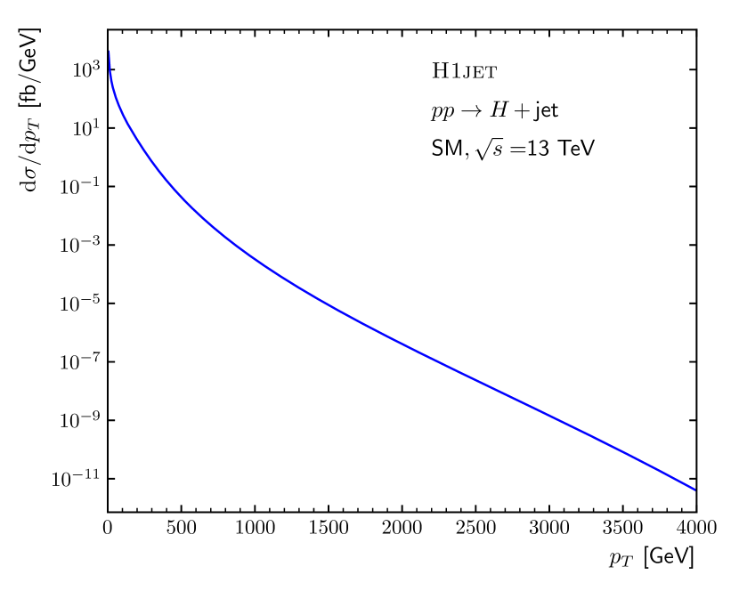
Figure 1: The $p_{T}$ distribution for the SM process $pp\rightarrow H+\text{jet}$ from H1jet with default settings.

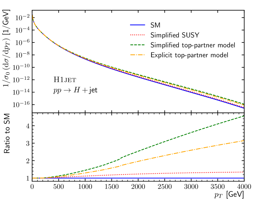
Figure 2: Comparison between the CP-even Higgs $p_{T}$ distributions for various built-in models.

4 Benchmarking

The various processes implemented in H1jet have been compared to those of SusHi [17, 18], and have all been found to be in agreement. The relative ratio between the H1jet result and the SusHi result for the $p_{T}$ distribution for the CP-odd Higgs are shown in Figure 3, and is found to be in agreement within the Monte Carlo error of SusHi for a large range of $p_{T}$ values. Overall the agreement with SusHi is within $3\times 10^{-4}$. Note that the largest discrepancies were observed in the low $p_{T}$ region. To validate the H1jet results we have compared them to the approximate expression valid at low $p_{T}$

$$\frac{d\sigma}{dp_{T}}\xrightarrow{p_{T}\,\rightarrow\,0}\sigma_{0}\left[4\,C_{A}\frac{\alpha_{s}}{\pi}\frac{1}{p_{T}}\left(\ln\frac{m_{H}}{p_{T}}+\mathcal{O}(1)\right)\right]\,,$$ (24)

where $\sigma_{0}$ is the total Born cross section for $gg\rightarrow H$. In Figure 4, we show $\frac{p_{T}}{\sigma_{0}}\left(\frac{\mathrm{d}\sigma}{\mathrm{d}p_{T}}\right)$ with the first term of eq. (24) subtracted, as a function of $\ln\frac{p_{T}}{m_{H}}$. For $p_{T}\rightarrow 0$ this goes nicely towards a constant as expected.

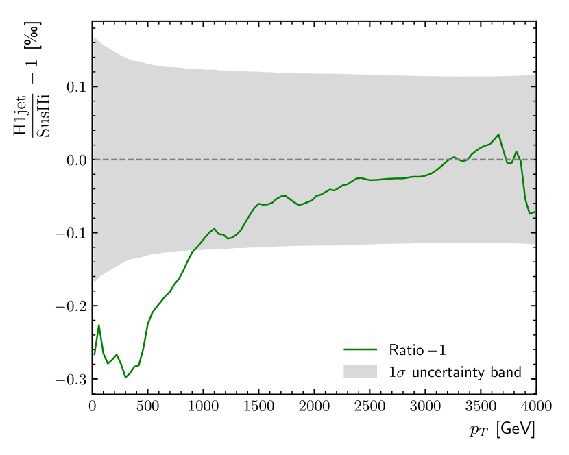
Figure 3: The relative difference in permille between the H1jet result and that of SusHi for the $p_{T}$ distribution for a CP-odd Higgs. The grey band indicates the Monte Carlo error of SusHi.

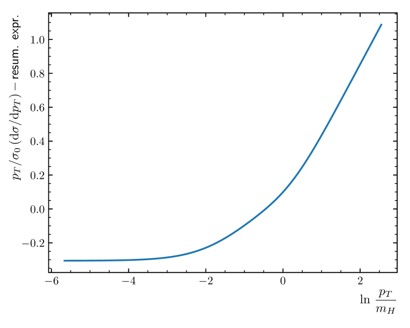
Figure 4: The CP-odd distribution $\frac{p_{T}}{\sigma_{0}}\left(\frac{\mathrm{d}\sigma}{\mathrm{d}p_{T}}\right)$ with the first term of the $p_{T}$ resummation subtracted, as a function of $\ln\frac{p_{T}}{m_{H}}$. For low $p_{T}$ values it convergences to a constant value.

The relative ratio between the H1jet and SusHi results for the SUSY are shown in Figure 5 and is within $2\times 10^{-4}$. Again the low $p_{T}$ behaviour can be checked by comparing to the resummed expression in Figure 6.

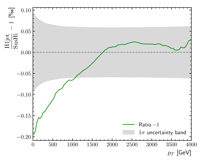
Figure 5: The relative difference in permille between the H1jet result and that of SusHi for the $p_{T}$ distribution in SUSY. The grey band indicates the Monte Carlo error of SusHi.

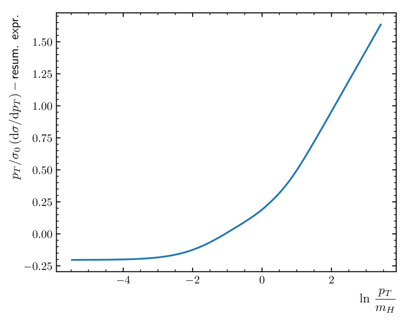
Figure 6: The SUSY distribution $\frac{p_{T}}{\sigma_{0}}\left(\frac{\mathrm{d}\sigma}{\mathrm{d}p_{T}}\right)$ with the first term of the $p_{T}$ resummation subtracted, as a function of $\ln\frac{p_{T}}{m_{H}}$. For low $p_{T}$ values it convergences to a constant value.

Note that our numerical accuracy crucially depends not only on the accuracy of the numerical integration, but of that of the auxiliary programs used to compute the PDF evolution (HOPPET) and the scalar integrals (CHAPLIN). We have modified various internal parameters of the two libraries, and we obtained differences that are less than permille level. So, a conservative estimate of the numerical uncertainty of H1jet is $1\times 10^{-3}$.

5 Adding New Processes to H1jet

H1jet can be interfaced to use the squared matrix element evaluated from a custom Fortran code. The implementation may be most easily explained with a specific example. This section should be read very carefully before attempting to use the interface.

5.1 Example: Axion-Like-Particle (ALP) Effective Theory

We will present here a specific example of adding to H1jet the production of a light axion-like-particle (ALP), $a$, along with a jet. For simplicity, we only consider the gluon-fusion channel,

$$gg\rightarrow ga\,.$$ (25)

This is a tree-level process due to an effective ALP-gluon coupling,

$$\delta\mathcal{L}_{a}\supset-c_{\tilde{G}}\frac{a}{f_{a}}G_{\mu\nu}^{a}\tilde{G}^{a\mu\nu}\,,$$ (26)

where $G_{\mu\nu}^{a}$ is the gluon field strength tensor and $\tilde{G}^{a}_{\mu\nu}=(1/2)\epsilon_{\mu\nu\rho\sigma}{G}^{a\rho\sigma}$ its dual. The model and the FeynRules [30] model files are described and provided in ref. [31]. We use FeynCalc [32, 33, 34] to evaluate the amplitude from the model, so we have to convert the FeynRules model to a FeynArts [35] model in Mathematica:

• << FeynRules‘

• LoadModel["SM.fr", "alp_linear.fr", "alp_linear_operators.fr"];

• WriteFeynArtsOutput[LSM + LALP, CouplingRename -> False];

The resulting FeynArts model files are written to a new directory ALP_linear_FA, which needs to be moved to the FeynArts/Models directory. Note that in the FeynArts model, the ALP field is called S[4] and the gluon fields are called V[4].

In a new Mathematica session, we load FeynCalc with FeynArts:

• $LoadAddOns = {"FeynArts"};

• << FeynCalc‘

The FeynArts/Models directory can be located with:

• $FeynArtsDir

First, we patch the ALP_linear_FA model with:

• FAPatch[PatchModelsOnly -> True]

This ensures that the model files works with FeynCalc.

Then we create the tree-level $2\rightarrow 2$ topologies and insert the relevant fields for our process:

• tops = CreateTopologies[0, 2 -> 2];

• ins = InsertFields[tops, {V[4], V[4]} -> {V[4], S[4]}, InsertionLevel -> {Classes}, Model -> "ALP_linear_FA", GenericModel -> "ALP_linear_FA"];

It is possible to draw the Feynman diagrams for the process as a check:

• Paint[ins, ColumnsXRows -> {2, 1}, Numbering -> Simple, SheetHeader -> None,      ImageSize -> {512, 256}];

We then set up the amplitude:

• feynamp = CreateFeynAmp[ins];

• amp = FCFAConvert[feynamp, IncomingMomenta -> {k1, k2}, OutgoingMomenta -> {k3, k4},                  UndoChiralSplittings -> True, ChangeDimension -> 4,                  TransversePolarizationVectors -> {k1, k2, k3}, List -> False,                  SMP -> True, Contract -> True, DropSumOver -> True]

While not strictly necessary, it is recommended to enable the SMP option. Any additional substitutions in the amplitude can be specified with the FinalSubstitutions option.

We then set up the kinematics:

• FCClearScalarProducts[];

• SetMandelstam[s, t, u, k1, k2, -k3, -k4, 0, 0, 0, mA];

We introduce here a parameter mA for the ALP mass $m_{a}$.

We then square the amplitude:

• ampsquared = Simplify[  (TrickMandelstam[#1, {s, t, u, mA^2}] & )[    (DoPolarizationSums[#1, k2, k1, ExtraFactor -> 1/2] & )[      (DoPolarizationSums[#1, k1, k2, ExtraFactor -> 1/2] & )[        (DoPolarizationSums[#1, k3, 0] & )[          (SUNSimplify[#1, Explicit -> True, SUNNToCACF -> False] & )[            FeynAmpDenominatorExplicit[(1 / (SUNN^2 - 1)^2) * (amp * ComplexConjugate[amp])]]]]]]] /. SUNN -> 3

Setting the SUNNToCACF option in SUNSimplify[] to False is not necessary, nor is it necessary to fix SUNN to $3$. This can be handled by the dressing script and H1jet.

Finally, we write the amplitude as Fortran code to a file:

• Write2["ALP_amp.f90", gg = ampsquared, FormatType -> FortranForm, FortranFormatDoublePrecision -> False]

Note here that we specify the gluon-gluon channel with the gg = ampsquared input to the function. This is required for the subsequent dressing script to work properly. It is important to specify the $2$-particle initial state by using combinations of g, u, d, c, s, b, ubar, dbar, cbar, sbar, and bbar. One can also use q and qbar for all the light quarks and antiquarks respectively, i.e. $u$, $d$, $c$, and $s$. For example, bbbar will be the $b\bar{b}$ channel.

The generated Fortran code ALP_amp.f90 has the following content:

⬇

gg = (3.*CGtil**2*(mA**8 - 2.*mA**6*(t + u) +

& 3.*mA**4*(t + u)**2 - 2.*mA**2*(t + u)**3 +

& (t**2 + t*u + u**2)**2)*SMP("g_s")**2)/

& (fa**2*s*t*u)

This code has to be dressed by the Python helper script DressUserAmpCode.py:

⬇

python DressUserAmpCode.py ALP_amp.f90

This produces a dressed Fortran code file called by default user_interface.f90.

The helper script provides a help message which can be called with -h or --help. The name of the output file can be specified with the -o option. Multiple input Fortran files can be given as arguments to the helper script. The full usage is:

⬇

python DressFeynCalcCode.py [-h] [-o [OUTFILE]] inputfile [inputfile ...]

The provided input Fortran code files does not necessarily have to be generated with FeynCalc. They can be generated by any other program or even be written by hand by providing the appropriate expression for gg or the desired channel.

To use the new dressed custom Fortran code with H1jet, it is necessary to recompile H1jet with the custom Fortran code:

⬇

./configure USERFILE=/path/to/custom/user_interface.f90

make clean

make

Running ./h1jet --help we see that three new additional options have been added:

--c_CGtil <value>

The Wilson coefficient $c_{\tilde{G}}$ in eq. (26).

--c_mA <value>

The ALP mass, $m_{a}$.

--c_fa <value>

The ALP suppression scale $f_{a}$ in eq. (26).

The leading c_ in the name stands for “custom” and is automatically added in order to avoid naming issues in the code.

The result from the ALP implementation in H1jet is shown in Figure 7 and can be compared to the H1jet result for the CP-odd Higgs by using a single top quark in the loop with an infinite mass limit, resulting in an effective coupling between the CP-odd Higgs and the gluons. In fact, the respective ALP and CP-odd couplings are then related as such,

$$\frac{c_{\tilde{G}}^{2}}{f_{a}^{2}}=\frac{\alpha_{s}^{2}}{64\pi^{2}v^{2}}\,.$$ (27)

The comparison is shown in Figure 8, where we see agreement within $4\times 10^{-6}$.

The result can also be compared to the same FeynRules model used with MadGraph5_aMC@NLO [16], where our code takes one second to run, while MadGraph can take up to several hours depending on the number of events, due to MadGraph running a full Monte Carlo integration. We have found that H1jet agrees with MadGraph5_aMC@NLO within Monte Carlo errors. We have also seen that MadGraph5_aMC@NLO runs into numerical instabilities at low $p_{T}$, while H1jet has by construction the correct behaviour.

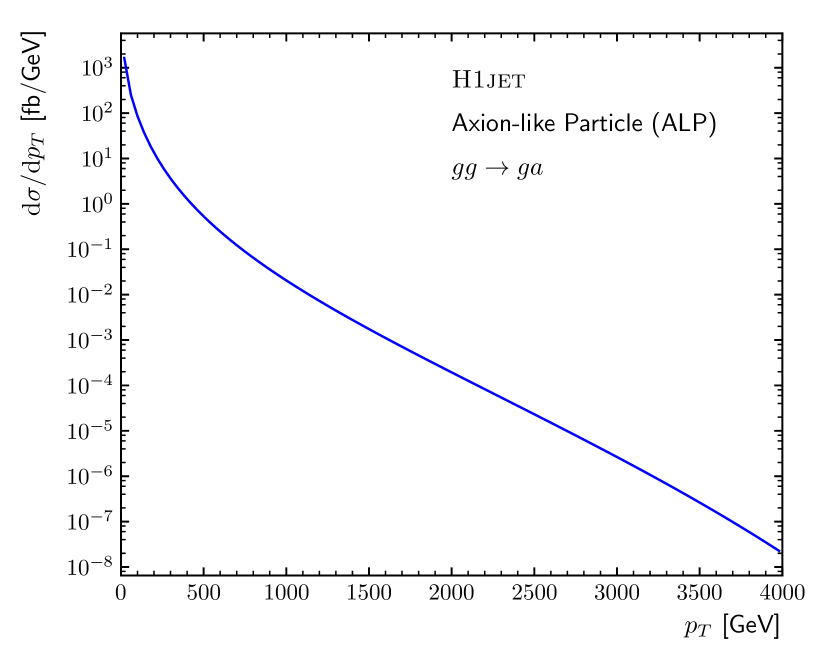
Figure 7: The $p_{T}$ distribution for the process $gg\rightarrow ga$ from H1jet with the amplitude from the user interface.

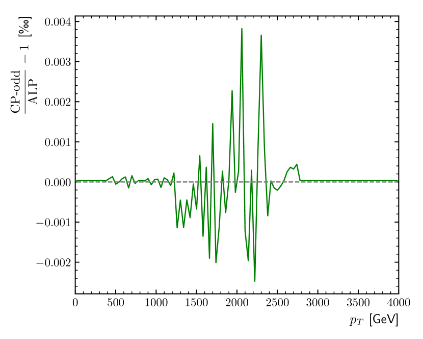
Figure 8: The relative ratio in permille between the CP-odd result and the result with the amplitude from the user interface.

5.1.1 The Total Cross Section

While not strictly necessary for the user interface to run, it is still recommended to add the code for the evaluation of the total cross section to the custom user interface. This is easy to do as well. We will here show it for the ALP model.

We start with considering the gluon-fusion ALP production, $gg\rightarrow a$. In Mathematica, create a tree-level $2\rightarrow 1$ topology, and insert the fields:

• tops = CreateTopologies[0, 2 -> 1];

• ins = InsertFields[tops, {V[4], V[4]} -> {S[4]}, InsertionLevel -> {Classes}, Model -> "ALP_linear_FA", GenericModel -> "ALP_linear_FA"];

Then we set up the amplitude:

• feynamp = CreateFeynAmp[ins];

• amp = FCFAConvert[feynamp, IncomingMomenta -> {k1, k2},                  OutgoingMomenta -> {k3}, UndoChiralSplittings -> True,                  ChangeDimension -> 4, TransversePolarizationVectors -> {k1, k2},                  List -> False, SMP -> True, Contract -> True, DropSumOver -> True]

as well as the kinematics:

• FCClearScalarProducts[];

• SP[k1, k1] = 0;

• SP[k2, k2] = 0;

• SP[k3, k3] = mA^2;

• SP[k1, k2] = mA^2 / 2;

We then square the amplitude:

• ampsquared = Simplify[  (DoPolarizationSums[#1, k2, k1, ExtraFactor -> 1/2] & )[    (DoPolarizationSums[#1, k1, k2, ExtraFactor -> 1/2] & )[      (SUNSimplify[#1, Explicit -> True, SUNNToCACF -> False] & )[        FeynAmpDenominatorExplicit[(1 / (SUNN^2 - 1)^2) * (amp * ComplexConjugate[amp])]]]]]

For a $2\rightarrow 1$ process, the hadronic cross section is given in eq. (4), where the partonic luminosity $\mathcal{L}_{gg}$ is handled by H1jet. Hence, we need to multiply our squared matrix element by

• xsec = Pi * ampsquared / mA^4

Finally, we can write the cross section as a Fortran code file:

• Write2["ALP_xsec.f90", xsgg = xsec, FormatType -> FortranForm, FortranFormatDoublePrecision -> False]

We again specify the gluon-gluon channel with the xsgg = xsec, but this time indicate with the leading xs that the code is for the Born cross section. Otherwise, the same rules apply. It is crucial to make sure not to save the Born cross section in the same file as the squared amplitude code for the transverse momentum distribution.

The new generated code ALP_xsec.f90 is provided to DressUserAmpCode.py along with the squared amplitude code:

⬇

python DressUserAmpCode.py ALP_amp.f90 ALP_xsec.f90

And H1jet can be recompiled to include the new source code:

⬇

./configure USERFILE=/path/to/custom/user_interface.f90

make clean

make

After which H1jet will calculate the Born cross section for the custom process.

6 Conclusions

We have presented a method that allows a fast computation of the transverse momentum distribution of a colour singlet. The method is implemented in the program H1jet, which returns a transverse momentum spectrum for the specified colour singlet in about a second. H1jet is similar in spirit to SusHi, but is incomparably faster.

The program implements various processes, including Higgs production both in gluon fusion and bottom-antibottom annihilation, as well as $Z$ production. Loop-induced Higgs production is implemented not only in the SM, but also in attractive BSM scenarios, such as SUSY or composite Higgs. For SUSY, we implement a simplified model with two stops, as done in ref. [29]. For composite Higgs, we implement both the simplified model of ref. [10], as well as some explicit models with one or more top partners [27]. Loop integrals can be computed either exactly or in the infinite-mass limit. The latter limit implements in practice a dimension-6 contact interaction between the Higgs and the gluon field. The program is very flexible, and the only process-dependent input is the corresponding amplitude in terms of Mandelstam invariants. This can be computed by the user either manually, or with the use of automated programs such as FeynCalc [34], and connected to the program via a simple interface. As an example, we have included in the package the calculation of the transverse momentum distribution of an ALP starting from the general Feynman rules of ref. [31]. Note that the possibility of automatically implementing a new model inside the program is a feature that is not available in SusHi. We also stress that it is also possible to take advantage of input files to obtain results for an arbitrary number of fermions and scalars in loops, with appropriate couplings. This could be used, for instance, to implement the MSSM instead of the provided simplified SUSY model.

We stress that H1jet is not a replacement for a proper Monte Carlo analysis implementing realistic experimental cuts. However, we believe it will be invaluable for BSM experts to assess whether a given model gives sizeable deviations from the SM. In fact, due to its fast implementation, H1jet makes it possible to perform parameter scans in seconds, and to take into account mass effects in specific models. Also, due to the fact that H1jet is not based on a Monte Carlo integration, one can separate interference between different contributions very precisely, something which is very difficult to achieve with Monte Carlo event generators.

H1jet can be also useful to precision phenomenology. In fact, it makes it possible to easily perform theoretical studies of the transverse momentum distribution of a colour singlet, especially those involving the matching of resummed calculations with exact fixed order. Also, although the implemented cross sections are computed at the lowest order in QCD, nothing prevents the inclusion of higher orders, provided one integrates over all coloured particles.

Acknowledgements.

The idea of having a fast program to compute transverse momentum spectra started from AB’s collaboration with G. Zanderighi, P. F. Monni and F. Caola. AB acknowledges many useful discussions with them on the topic. AB also wishes to thank B. Dillon, W. Ketaiam and S. Kvedaraitė for contributions to a private preliminary version of H1jet. We thank J. M. Lindert for all his helpful remarks and suggestions on this paper. The studentship of AL is supported by the Science Technology and Facilities Council (STFC) under grant number ST/P000819/1. The work of AB is supported by the Science Technology and Facilities Council (STFC) under grants number ST/P000819/1 and ST/T00102X/1.

Appendix A Implementation of Scalar Integrals

This appendix contains the details of how H1jet computes one-loop scalar integrals that are relevant for Higgs production. These integrals depend on one internal mass, which we denote by $m$, and are functions of Mandelstam invariants.

Scalar integrals can be written in terms of logarithms and dilogarithms of complex arguments, which require appropriate analytic continuations. Instead of performing such manipulations ourselves, we have decided to use the implementation of the library CHAPLIN, and recast all relevant transcendental functions into harmonic polylogarithms $H(\vec{a};z)$, with $\vec{a}=(a_{1},\dots,a_{n})$. For real values of the argument of a polylogarithm, CHAPLIN uses the $+i\varepsilon$ prescription, i.e. $H(\vec{a};z)$ with $z$ real is interpreted as $H(\vec{a};z+i\varepsilon)$. Therefore, we need to make sure that the imaginary part of the argument of scalar integrals is consistent with the convention of CHAPLIN.

The relevant one-loop integrals we need to deal with are bubbles, triangles and boxes.

Bubbles.

The bubble integral is defined as

$$B_{0}(s)=2-\sqrt{1-\frac{4(m^{2}-i\varepsilon)}{s}}\ln\left[-\frac{z}{1-z}\right]\,,$$ (28)

where

$$z=\frac{1}{2}\left(1+\sqrt{1-\frac{4(m^{2}-i\varepsilon)}{s}}\right)\,.$$ (29)

The argument of the logarithm in eq. (28) has a different form according to the value of $s$:

$$-\frac{z}{1-z}=\left\{\begin{split}&-\frac{1+\sqrt{1+\frac{4m^{2}}{|s|}}}{1-\sqrt{1+\frac{4m^{2}}{|s|}}}\,,\qquad\qquad s<0\,,\\ &-\frac{1+i\sqrt{\frac{4m^{2}}{s}-1}}{1-i\sqrt{\frac{4m^{2}}{s}-1}}\,,\qquad\quad\>\>0<s<4m^{2}\,,\\ &-\frac{1-\sqrt{1-\frac{4m^{2}}{s}}}{1-\sqrt{1-\frac{4m^{2}}{s}}}-i\varepsilon\,,\qquad s>4m^{2}\end{split}\right.$$ (30)

Note that the only case in which one needs a small imaginary part is the case $s>4m^{2}$. This imaginary part has the opposite convention as in CHAPLIN. As a solution, we invert the argument of the logarithm and use the identity $\ln z=-\ln(1/z)$. In practice, after an appropriate analytic continuation of the square root, we define

$$z\equiv\left\{\begin{split}\frac{1}{2}\left(1+\sqrt{1-\frac{4m^{2}}{s}}\right)\,,&\qquad\frac{4m^{2}}{s}<1\\ \frac{1}{2}\left(1+i\sqrt{\frac{4m^{2}}{s}-1}\right)\,,&\qquad\frac{4m^{2}}{s}>1\end{split}\right.$$ (31)

and implement the bubble as follows:

$$B_{0}(s)=2-(2z-1)\,H\left(1;\frac{1}{z}\right)\,.$$ (32)

Note that a logarithm of a negative number can also be correctly analytically continued by using the default Fortran implementation of the complex logarithm. As for CHAPLIN, Fortran assumes that a negative number has a small positive imaginary part. Therefore, in case we have a small negative imaginary part, we can still use the relation $\ln z=-\ln(1/z)$, which gives the correct analytic continuation.

Triangles.

The triangle integral $C_{0}(s)$ is defined as

$$C_{0}(s)=\frac{1}{2s}\ln^{2}\left[-\frac{z}{1-z}\right]\,,$$ (33)

where $z$ is given in eq. (29). Again, for $s>4m^{2}$, the argument of the logarithm has the opposite sign with respect to what is implicitly assumed by CHAPLIN. Therefore, we invert again the argument of the logarithm, and using the definition of $z$ in eq. (31), we implement the triangle as follows:

$$s\,C_{0}(s)=H\left(1,1;\frac{1}{z}\right)\,.$$ (34)

Boxes.

The scalar four-point function with three massless (the gluons) and one massive (the Higgs boson) external lines is given by [25],

$$D(s,t)=\frac{1}{st}\int_{0}^{1}\frac{\mathrm{d}x}{x(1-x)+m^{2}u/(ts)}\left[-\ln\left(1-i\varepsilon-\frac{m_{H}^{2}}{m^{2}}x(1-x)\right)\right.\\ \left.+\ln\left(1-i\varepsilon-\frac{s}{m^{2}}x(1-x)\right)+\ln\left(1-i\varepsilon-\frac{t}{m^{2}}x(1-x)\right)\right]\,,$$ (35)

which can be expressed in terms of complex dilogarithms by using the exact result

$$\frac{1}{st}\int_{0}^{1}\frac{dx}{x(1-x)+m^{2}u/(ts)}\ln\left(1-i\varepsilon-\frac{v}{m^{2}}x(1-x)\right)=\frac{2}{\sqrt{1+4m^{2}u/(ts)}}\times\\ \times\left[\mathrm{Li}_{2}\left(\frac{x_{-}}{x_{-}-y}\right)-\mathrm{Li}_{2}\left(\frac{x_{+}}{x_{+}-y}\right)+\mathrm{Li}_{2}\left(\frac{x_{-}}{y-x_{+}}\right)-\mathrm{Li}_{2}\left(\frac{x_{+}}{y-x_{-}}\right)\right.\\ \left.+\ln\left(\frac{-x_{-}}{x_{+}}\right)\ln\left(1-i\varepsilon-\frac{v}{m^{2}}x_{-}x_{+}\right)\right]\,,$$ (36)

where

$$x_{\pm}\equiv\frac{1}{2}\left(1\pm\sqrt{1+\frac{4m^{2}u}{ts}}\right)$$ (37)

are real numbers, with $x_{+}>1$ and $x_{-}<0$, and

$$y\equiv\frac{1}{2}\left(1+\sqrt{1-\frac{4(m^{2}-i\varepsilon)}{v}}\right)\,,$$ (38)

acquires an imaginary part according to the value of $v$. In particular, keeping track of the imaginary part of $y$ yields

$$y=\left\{\begin{split}\frac{1}{2}\left(1+\sqrt{1+\frac{4m^{2}}{|v|}}\right)-i\varepsilon\,,&\qquad v<0\\ \frac{1}{2}\left(1+i\sqrt{\frac{4m^{2}}{v}-1}\right)\,,&\qquad 0<v<4m^{2}\\ \frac{1}{2}\left(1+\sqrt{1-\frac{4m^{2}}{v}}\right)+i\varepsilon\,,&\qquad v>4m^{2}\end{split}\right.$$ (39)

From the above, we see that w for $0<v<4m^{2}$ we can use the dilogarithms as given by CHAPLIN. For $v<0$, $x_{-}/(x_{-}-y)$ and $x_{+}/(y-x_{-})$ acquire a small positive imaginary part, whereas $x_{+}/(x_{+}-y)$ and $x_{-}/(y-x_{+})$ a small negative imaginary part. The reverse happens for $v>4m^{2}$. Therefore, we need to perform some formal manipulations to use the harmonic polylogarithms provided by CHAPLIN.

In practice, whenever the argument $z$ of the dilogarithm is complex, we just use the definitory relation $\mathrm{Li_{2}}(z)=H(0,1;z)$. When $z=x+i\varepsilon$, with $x$ real, we use $\mathrm{Li_{2}}(x+i\varepsilon)=H(0,1;x)$, with $H(0,1;x)$ the complex number provided by CHAPLIN. If $z=x-i\varepsilon$, we use the identities

$$\begin{split}\mathrm{Li}_{2}\left(x-i\varepsilon\right)&=-H\left(0,1;\frac{1}{x}\right)-\frac{\pi^{2}}{6}-H(0,0;-x)=-H(0,-1;-x)=\\ &=-H\left(0,1,1-x\right)+\frac{\pi^{2}}{6}+H(1;1-x)H(-1;-x)\,,\end{split}$$ (40)

and we select the one that gives the smallest imaginary part. This of course give numerically indistinguishable results when the imaginary part is large, but is of crucial importance when the imaginary part should be zero but it is not because of the specific numerical methods employed by CHAPLIN.

References

- [1] https://h1jet.hepforge.org/.
- [2] ATLAS Collaboration, G. Aad et al., “Observation of a new particle in the search for the Standard Model Higgs boson with the ATLAS detector at the LHC,” Phys. Lett. B 716 (2012) 1–29, arXiv:1207.7214 [hep-ex].
- [3] CMS Collaboration, S. Chatrchyan et al., “Observation of a New Boson at a Mass of 125 GeV with the CMS Experiment at the LHC,” Phys. Lett. B 716 (2012) 30–61, arXiv:1207.7235 [hep-ex].
- [4] ATLAS Collaboration, G. Aad et al., “Combined measurements of Higgs boson production and decay using up to fb-1 of proton-proton collision data at 13 TeV collected with the ATLAS experiment,” Phys. Rev. D 101 no. 1, (2020) 012002, arXiv:1909.02845 [hep-ex].
- [5] CMS Collaboration, A. M. Sirunyan et al., “Combined measurements of Higgs boson couplings in proton–proton collisions at ,” Eur. Phys. J. C 79 no. 5, (2019) 421, arXiv:1809.10733 [hep-ex].
- [6] ATLAS Collaboration, M. Aaboud et al., “Combined measurement of differential and total cross sections in the and the decay channels at TeV with the ATLAS detector,” Phys. Lett. B 786 (2018) 114–133, arXiv:1805.10197 [hep-ex].
- [7] CMS Collaboration, A. M. Sirunyan et al., “Measurement and interpretation of differential cross sections for Higgs boson production at 13 TeV,” Phys. Lett. B 792 (2019) 369–396, arXiv:1812.06504 [hep-ex].
- [8] A. Azatov and A. Paul, “Probing Higgs couplings with high Higgs production,” JHEP 01 (2014) 014, arXiv:1309.5273 [hep-ph].
- [9] C. Grojean, E. Salvioni, M. Schlaffer, and A. Weiler, “Very boosted Higgs in gluon fusion,” JHEP 05 (2014) 022, arXiv:1312.3317 [hep-ph].
- [10] A. Banfi, A. Martin, and V. Sanz, “Probing top-partners in Higgs+jets,” JHEP 08 (2014) 053, arXiv:1308.4771 [hep-ph].
- [11] ATLAS Collaboration, G. Aad et al., “ Properties of Higgs Boson Interactions with Top Quarks in the and Processes Using with the ATLAS Detector,” Phys. Rev. Lett. 125 no. 6, (2020) 061802, arXiv:2004.04545 [hep-ex].
- [12] CMS Collaboration, A. M. Sirunyan et al., “Measurements of Production and the CP Structure of the Yukawa Interaction between the Higgs Boson and Top Quark in the Diphoton Decay Channel,” Phys. Rev. Lett. 125 no. 6, (2020) 061801, arXiv:2003.10866 [hep-ex].
- [13] F. Maltoni, E. Vryonidou, and C. Zhang, “Higgs production in association with a top-antitop pair in the Standard Model Effective Field Theory at NLO in QCD,” JHEP 10 (2016) 123, arXiv:1607.05330 [hep-ph].
- [14] CMS Collaboration, A. M. Sirunyan et al., “Search for dark matter produced with an energetic jet or a hadronically decaying W or Z boson at TeV,” JHEP 07 (2017) 014, arXiv:1703.01651 [hep-ex].
- [15] ATLAS Collaboration, M. Aaboud et al., “Constraints on mediator-based dark matter and scalar dark energy models using TeV collision data collected by the ATLAS detector,” JHEP 05 (2019) 142, arXiv:1903.01400 [hep-ex].
- [16] J. Alwall, R. Frederix, S. Frixione, V. Hirschi, F. Maltoni, O. Mattelaer, H. S. Shao, T. Stelzer, P. Torrielli, and M. Zaro, “The automated computation of tree-level and next-to-leading order differential cross sections, and their matching to parton shower simulations,” JHEP 07 (2014) 079, arXiv:1405.0301 [hep-ph]. https://launchpad.net/mg5amcnlo.
- [17] R. V. Harlander, S. Liebler, and H. Mantler, “SusHi: A program for the calculation of Higgs production in gluon fusion and bottom-quark annihilation in the Standard Model and the MSSM,” Comput. Phys. Commun. 184 (2013) 1605–1617, arXiv:1212.3249 [hep-ph].
- [18] R. V. Harlander, S. Liebler, and H. Mantler, “SusHi Bento: Beyond NNLO and the heavy-top limit,” Comput. Phys. Commun. 212 (2017) 239–257, arXiv:1605.03190 [hep-ph]. https://sushi.hepforge.org.
- [19] G. P. Salam and J. Rojo, “A Higher Order Perturbative Parton Evolution Toolkit (HOPPET),” Comput. Phys. Commun. 180 (2009) 120–156, arXiv:0804.3755 [hep-ph]. https://hoppet.hepforge.org/.
- [20] A. Banfi, F. Caola, F. A. Dreyer, P. F. Monni, G. P. Salam, G. Zanderighi, and F. Dulat, “Jet-vetoed Higgs cross section in gluon fusion at N3LO+NNLL with small- resummation,” JHEP 04 (2016) 049, arXiv:1511.02886 [hep-ph]. https://jetvheto.hepforge.org/.
- [21] A. Buckley, J. Ferrando, S. Lloyd, K. Nordström, B. Page, M. Rüfenacht, M. Schönherr, and G. Watt, “LHAPDF6: parton density access in the LHC precision era,” Eur. Phys. J. C 75 (2015) 132, arXiv:1412.7420 [hep-ph]. https://lhapdf.hepforge.org/.
- [22] S. Buehler and C. Duhr, “CHAPLIN - Complex Harmonic Polylogarithms in Fortran,” Comput. Phys. Commun. 185 (2014) 2703–2713, arXiv:1106.5739 [hep-ph]. https://chaplin.hepforge.org/.
- [23] H. Georgi, “Effective field theory and electroweak radiative corrections,” Nucl. Phys. B 363 (1991) 301–325.
- [24] M. Spira, A. Djouadi, D. Graudenz, and P. Zerwas, “Higgs boson production at the LHC,” Nucl. Phys. B 453 (1995) 17–82, arXiv:hep-ph/9504378.
- [25] U. Baur and E. Glover, “Higgs Boson Production at Large Transverse Momentum in Hadronic Collisions,” Nucl. Phys. B 339 (1990) 38–66.
- [26] G. Corcella, I. Knowles, G. Marchesini, S. Moretti, K. Odagiri, P. Richardson, M. Seymour, and B. Webber, “HERWIG 6: An Event generator for hadron emission reactions with interfering gluons (including supersymmetric processes),” JHEP 01 (2001) 010, arXiv:hep-ph/0011363.
- [27] A. Banfi, B. M. Dillon, W. Ketaiam, and S. Kvedaraite, “Composite Higgs at high transverse momentum,” JHEP 01 (2020) 089, arXiv:1905.12747 [hep-ph].
- [28] J. F. Gunion and H. E. Haber, “The CP conserving two Higgs doublet model: The Approach to the decoupling limit,” Phys. Rev. D 67 (2003) 075019, arXiv:hep-ph/0207010.
- [29] A. Banfi, A. Bond, A. Martin, and V. Sanz, “Digging for Top Squarks from Higgs data: from signal strengths to differential distributions,” JHEP 11 (2018) 171, arXiv:1806.05598 [hep-ph].
- [30] A. Alloul, N. D. Christensen, C. Degrande, C. Duhr, and B. Fuks, “FeynRules 2.0 - A complete toolbox for tree-level phenomenology,” Comput. Phys. Commun. 185 (2014) 2250–2300, arXiv:1310.1921 [hep-ph]. https://feynrules.irmp.ucl.ac.be.
- [31] I. Brivio, M. Gavela, L. Merlo, K. Mimasu, J. No, R. del Rey, and V. Sanz, “ALPs Effective Field Theory and Collider Signatures,” Eur. Phys. J. C 77 no. 8, (2017) 572, arXiv:1701.05379 [hep-ph]. https://feynrules.irmp.ucl.ac.be/wiki/ALPsEFT.
- [32] R. Mertig, M. Bohm, and A. Denner, “FEYN CALC: Computer algebraic calculation of Feynman amplitudes,” Comput. Phys. Commun. 64 (1991) 345–359.
- [33] V. Shtabovenko, R. Mertig, and F. Orellana, “New Developments in FeynCalc 9.0” Comput. Phys. Commun. 207 (2016) 432–444, arXiv:1601.01167 [hep-ph].
- [34] V. Shtabovenko, R. Mertig, and F. Orellana, “FeynCalc 9.3: New features and improvements,” Comput. Phys. Commun. 256 (2020) 107478, arXiv:2001.04407 [hep-ph]. https://feyncalc.github.io.
- [35] T. Hahn, “Generating Feynman diagrams and amplitudes with FeynArts 3,” Comput. Phys. Commun. 140 (2001) 418–431, arXiv:hep-ph/0012260. http://www.feynarts.de.