DIPN: Deep Interaction Prediction Network with Application to Clutter Removal

Abstract

We propose a Deep Interaction Prediction Network (DIPN) for learning to predict complex interactions that ensue as a robot end-effector pushes multiple objects, whose physical properties, including size, shape, mass, and friction coefficients may be unknown a priori. DIPN “imagines” the effect of a push action and generates an accurate synthetic image of the predicted outcome. DIPN is shown to be sample efficient when trained in simulation or with a real robotic system. The high accuracy of DIPN allows direct integration with a grasp network, yielding a robotic manipulation system capable of executing challenging clutter removal tasks while being trained in a fully self-supervised manner. The overall network demonstrates intelligent behavior in selecting proper actions between push and grasp for completing clutter removal tasks and significantly outperforms the previous state-of-the-art. Remarkably, DIPN achieves even better performance on the real robotic hardware system than in simulation. Videos, code, and experiments log are available at https://github.com/rutgers-arc-lab/dipn.

I Introduction

We propose a Deep Interaction Prediction Network (DIPN) for learning object interactions directly from examples and using the trained network for accurately predicting the poses of the objects after an arbitrary push action (Fig. 1). To demonstrate its effectiveness, We integrate DIPN with a deep Grasp Network (GN) for completing challenging clutter removal manipulation tasks. Given grasp and push actions to choose from, the objective is to remove all objects from the scene/workspace with a minimum number of actions. In an iteration of push/pick selection (Fig. 1c), the system examines the scene and samples a large number of candidate grasp and push actions. Grasps are immediately scored by GN, whereas for each candidate push action, DIPN generates an image corresponding to the predicted outcome. In a sense, DIPN “imagines” what happens to the current scene if the robot executes a certain push. The predicted future images are also scored by GN; the action with the highest expected score, either a push or a grasp, is then executed.

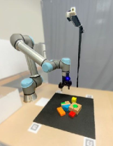
(a)

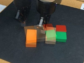
(b)

\begin{overpic}[width=433.62pt]{figures/system-architecture.pdf} \footnotesize\put(24.5,38.0){State observation} \put(14.5,13.0){\makebox(0.0,0.0)[]{Deep Interaction}} \put(14.5,9.0){\makebox(0.0,0.0)[]{Prediction Network}} \put(14.5,4.5){\makebox(0.0,0.0)[]{({DIPN})}} \put(50.0,4.0){\makebox(0.0,0.0)[]{Predicted states after push}} \put(85.25,35.0){\makebox(0.0,0.0)[]{Deep}} \put(85.25,31.0){\makebox(0.0,0.0)[]{Grasp Network}} \put(85.25,26.5){\makebox(0.0,0.0)[]{({GN})}} \put(85.25,9.5){\makebox(0.0,0.0)[]{Grasp or push}} \put(85.25,6.0){\makebox(0.0,0.0)[]{action}} \end{overpic}

(c)

Figure 1: (a) The system setup includes a workspace with objects to remove, a Universal Robots UR-5e manipulator with a Robotiq 2F-85 two-finger gripper, and an Intel RealSense D435 RGB-D camera. (b) An example push action and superimposed images of scenes before and after the push. (c) System architecture of our pipeline, and one predicted image that DIPN can generate for the push shown in (b). Notice the similarity between the predicted synthetic image and the real image resulting from the push action.

Our extensive evaluation demonstrates that DIPN can accurately predict objects’ poses after a push action with collisions, resulting in less than $10\%$ average single object pose error in terms of IoU (Intersection-over-Union), a significant improvement over the compared baselines. Push prediction by DIPN generates clear synthetic images that can be used by GN to evaluate grasp actions in future states. Together with GN, our entire pipeline achieves $34\%$ higher completion rate, $20.9\%$ higher grasp success rate, and $30.4\%$ higher action efficiency in comparison to [1] on challenging clutter removal scenarios. Moreover, experiments suggest that DIPN can learn from randomly generated scenarios with the learned policy maintaining high levels of performance on challenging tasks involving previously unseen objects. Remarkably, DIPN+GN achieves an even better performance on real robotic hardware than it does in simulation, within which it was developed.

II Related Work

Prehensile (e.g., grasping) and non-prehensile (e.g., pushing) manipulation techniques are typically studied separately in robotics [2, 3, 4, 5, 6, 7, 8, 9, 10, 11, 12, 13, 14, 15, 16, 17, 18, 19, 20, 21, 22, 23, 24, 25, 26, 27, 28, 29, 30, 31, 32, 33, 34, 35, 36, 37, 38, 39, 40]. Seeking to reap the benefit from the apparent synergy between push and grasp, recent years have seen increasing interests in using both to tackle challenging manipulation problems, including pre-grasp push [41, 42, 43, 44, 45] and more recently push-assisted grasping [1].

Grasping: Robotic grasping techniques can generally be categorized in two main categories: analytical and data-driven [2]. Until the last decade, the majority of grasping techniques required precise analytical and 3D models of objects in order to predict the stability of force-closure or form-closure grasps [3, 4, 5]. However, building accurate models of new objects is a challenging task that requires thoroughly scanning all the objects in advance. Moreover, important material properties such as mass and friction coefficients are generally unknown. Statistical learning of grasp actions is an alternative data-driven approach that has received increased attention in the recent years. Most data-driven methods focused on isolated objects [46, 6, 7, 8, 9, 10]. Learning to grasp in cluttered scenes was explored in recent works [47, 11, 12, 13, 14, 15]. For example, a convolutional neural network was trained in the popular work [11] to detect 6D grasping poses in point clouds. Such an approach suffers when multiple objects are mistaken for a single object. Another drawback is that using only grasp actions may be insufficient for handling dense clutter, making pre-grasp push actions necessary.

Pushing: Pushing is an example of non-prehensile actions that robots can apply on objects. As with grasping, there are two main categories of methods that predict the effect of a push action [16]. Analytical methods rely on mechanical and geometric models of the objects and utilize physics simulations to predict the motion of an object [17, 18, 19, 20, 21, 22]. Notably, Mason [18] derived the voting theorem to predict the rotation and translation of an object pushed by a point contact. A stable pushing technique when objects remain in contact was also proposed in [19]. These methods often make strong assumptions such as quasi-static motion and uniform friction coefficients and mass distributions. To deal with non-uniform frictions, a regression method was proposed in [48] for identifying the support points of a pushed object by dividing the support surface into a grid. The limit surface plays a crucial role in the mechanical models of pushing. It is a convex set of all friction forces and torques that can be applied on an object in quasi-static pushing. The limit surface is often approximated as an ellipsoid [23], or a higher-order convex polynomial [24, 25, 26]. An ellipsoid approximation was also used to simulate the motion of a pushed object to perform a push-grasp [28]. To overcome the rigid assumptions of analytical methods, statistical learning techniques predict how new objects behave under various pushing forces by generalizing observed motions in training examples. For example, a Gaussian process was used to solve this problem in [29], but was limited to isolated single objects. Most recent push prediction techniques rely on deep learning [30, 31, 32], which can capture a wider range of physical interactions from vision. Deep RL was also used for learning pushing strategies from images [35, 36, 37, 38]. Our approach differs from the previous ones in two important aspects. First, our approach learns to predict the simultaneous motions of multiple objects that collide with each other. Second, the push predictions are used to plan pushing directions that improve the performance of a clutter removal system.

Push-grasping: A pre-grasp sliding manipulation technique that was recently developed [49, 41, 50, 51, 52] performs a sequence of non-prehensile actions such as side-pushing and top-sliding to facilitate grasping. Most existing methods for pre-grasp push require the existence of predefined geometric and mechanical models of the target object [42, 43, 44, 45]. In contrast to these techniques, our approach does not require models of the objects. The present work improves upon the closely related Visual Pushing and Grasping (VPG) technique [1] notably by explicitly learning to predict how pushed objects move, and replacing model-free estimates of the Q-values of pushing actions with one-step lookaheads.

III Problem Formulation

We denote the clutter removal problem (Fig. 1a) as Pushing Assisted Grasping (PaG). In a PaG, the workspace of the manipulator is a square region containing multiple objects and the volume directly above it. A camera is placed on top of the workspace for state observation. Given camera images, all objects must be removed using two basic motion primitives, grasp, and push, with a minimum number of actions.

In our experimental setup, the workspace has a uniform background color and the objects have different shapes, sizes, and colors. The end-effector is a 2-finger gripper with a narrow stroke that is slightly larger than the smallest dimension of individual objects. Objects are removed one by one, which requires a sequence of push and grasp actions. When deciding on the next action, a state observation is given as an RGB-D image, re-projected orthographically, cropped to the workspace’s boundary, and down-sampled to $224\times 224$.

From the down-sampled image, a large set of candidate actions is generated by considering each pixel in the image as a potential center of a grasp action or initial contact point of a push action. A grasp action $a^{\text{grasp}}=(x,y,\theta)$ is a vertical top-down grasp centered at pixel position $(x,y)$ with the end-effector rotation set to $\theta$ around the vertical axis of the workspace; a grasped object is subsequently transferred outside of the workspace and removed from the scene. Similarly, a push action $a^{\text{push}}=(x,y,\theta)$ is a horizontal sweep motion that starts at $(x,y)$ and proceeds along $\theta$ direction for a constant distance. The orientation $\theta$ can be one of $16$ values evenly distributed between $0$ and $360$ degrees. That is, the entire action space includes $2\times 224\times 224\times 16$ different grasp/push actions.

The problem studied in this paper is defined as:

Problem 1.

Pushing Assisted Grasping (PaG). Given objects in clutter and under the described system setup, choose a sequence of push and grasp actions for removing all the objects, based only on images of the workspace, while minimizing the number of actions taken.

IV Methodology

We describe the Deep Interaction Prediction Network (DIPN), the Grasp Network (GN), and the integrated pipeline for solving PaG challenges.

IV-A Deep Interaction Prediction Network (DIPN)

The architecture of our proposed DIPN is outlined in Fig. 2. At a high level, given an image and a candidate push action as inputs, DIPN segments the image and then predicts 2D transformations (translations and rotations) for all objects, and particularly for those affected by the push action, directly or indirectly through a cascade of object-object interactions. A predicted image of the post-push scene is synthesized by applying the predicted transformations on the segments. We opted against an end-to-end, pixel-to-pixel method as such methods (e.g., [30]) often lead to blurry or fragmented images, which are not conducive to predicting the quality of a potential future grasp action.

\begin{overpic}[width=433.62pt]{figures/push-prediction-flowchart.pdf} \scriptsize\put(0.0,29.5){Input image $I$} \put(0.0,28.0){$224\times 224\times 3$} \put(17.0,19.0){Segmentation} \put(17.0,17.5){$224\times 224\times 1$} \put(89.5,18.0){Output image $\hat{I}$} \put(89.5,16.5){$224\times 224\times 4$} \put(47.5,27.5){Binary push action image $M_{p}$} \put(54.5,26.0){$224{\times}224{\times}\{0{,}1\}$} \put(90.0,27.5){Binary image $M_{I}$} \put(73.5,29.5){{\color[rgb]{1,.5,0}{$M_{p}$}}} \put(86.5,29.5){{\color[rgb]{1,.5,0}{$M_{I}$}}} \put(90.0,26.0){$224{\times}224{\times}{\{}0{,}1{\}}$} \put(22.3,28.5){\makebox(0.0,0.0)[]{Push action $p$}} \put(22.3,26.25){\makebox(0.0,0.0)[]{\scriptsize$(83,140,22.5^{\circ})$}} \put(7.0,10.0){Mask R-CNN} \put(33.5,21.5){\makebox(0.0,0.0)[]{\parbox{72.26999pt}{\centering Mask image$\{M_{i}\}$, \\ $60{\times}60{\times}\{0{,}1\}$, \\ center position $\{c_{i}\}$\@add@centering}}} \put(33.5,14.4){\makebox(0.0,0.0)[]{\scriptsize$(54,69)$}} \put(33.5,8.4){\makebox(0.0,0.0)[]{\scriptsize$(67,90)$}} \put(33.5,2.4){\makebox(0.0,0.0)[]{\scriptsize$(73,112)$}} \put(35.2,15.8){{\color[rgb]{1,.5,0}{$M_{1}$}}} \put(35.2,9.6){{\color[rgb]{1,.5,0}{$M_{2}$}}} \put(35.2,3.8){{\color[rgb]{1,.5,0}{$M_{3}$}}} \put(36.0,17.5){\scriptsize ResNet\textsubscript{2}} \put(41.0,26.0){\scriptsize MLP\textsubscript{1}} \put(38.5,14.5){\scriptsize MLP\textsubscript{2}} \put(52.5,24.4){\scriptsize MLP\textsubscript{3}} \put(52.5,18.4){\scriptsize MLP\textsubscript{4}} \put(52.5,12.4){\scriptsize MLP\textsubscript{4}} \put(42.7,22.0){Encoded} \put(42.7,16.0){Encoded} \put(42.7,10.1){Encoded} \put(42.7,4.1){Encoded} \put(59.8,22.2){\makebox(0.0,0.0)[]{\parbox{72.26999pt}{\scriptsize\centering Direct \\ transformation\@add@centering}}} \put(59.8,16.2){\makebox(0.0,0.0)[]{\parbox{72.26999pt}{\scriptsize\centering Interactive \\ transformation\@add@centering}}} \put(59.8,10.2){\makebox(0.0,0.0)[]{\parbox{72.26999pt}{\scriptsize\centering Interactive \\ transformation\@add@centering}}} \put(66.0,13.5){\scriptsize Add} \put(73.7,19.5){\makebox(0.0,0.0)[]{\scriptsize ResNet\textsubscript{1}}} \put(69.5,16.2){\scriptsize MLP\textsubscript{5}} \put(79.3,16.7){\makebox(0.0,0.0)[]{\scriptsize Transformation}} \put(79.3,14.5){\makebox(0.0,0.0)[]{\scriptsize$(0,0,0^{\circ})$}} \put(79.3,10.7){\makebox(0.0,0.0)[]{\scriptsize Transformation}} \put(79.3,8.5){\makebox(0.0,0.0)[]{\scriptsize$(18,-3,6^{\circ})$}} \put(79.3,4.7){\makebox(0.0,0.0)[]{\scriptsize Transformation}} \put(79.3,2.5){\makebox(0.0,0.0)[]{\scriptsize$(15,1,-3^{\circ})$}} \end{overpic}

Figure 2: DIPN flow with an example. The network components dedicated to an object are colored with the same as the object. We only show the full network for the blue triangle object; the instance-specific structures for the other objects share the same weights and are simplified as dashed lines. Components inside the orange dot line are the core of the DIPN. The output image is synthesized by applying the predicted transformations to the segments.

Segmentation. DIPN employs Mask R-CNN [53] for object segmentation (instance level only, without semantic segmentation). The resulting binary masks ($m_{i}$) and their centers ($c_{i}$), one per object, serve as the input to the push prediction module of DIPN. Our Mask R-CNN setup has two classes, one for the background and one for the objects. The network is trained from scratch in a self-supervised manner without any human intervention: objects are randomly dropped into the workspace, and data is automatically collected. Images that can be easily segmented into separate instances based on color/depth information (distinct color blobs) are automatically labeled by the system as single instances for training the Mask R-CNN. The self-trained Mask R-CNN can then accurately find edges in images of tightly packed scenes and even in scenes with novel objects. Note that the data used for training the segmentation module are also counted in our evaluation of the data efficiency of our technique and the comparisons to alternative techniques.

Push sampling. Based on foreground segmentation, candidate push actions are generated by uniformly sampling push contact locations on the contour of object bundles (see the figure to the right). Push directions point to the centers of the objects. Pushes that cannot be performed physically, e.g., from the inside of an object bundle or in narrow spaces between objects, are filtered out based on the masks returned by R-CNN. In the figure, for example, samples between the two object bundles are deleted. A sampled push is defined as $p=(x,y,\theta)\in SE(2)$ where $x$, $y$ are the start location of the push and $\theta$ indicates the horizontal push direction. The push distance is fixed.

Input to push prediction. The initial scene image $I$, scene object masks and centers $(m_{i},c_{i})$, and a sampled push action $p=(x,y,\theta)$ are the main inputs to the push prediction module. To reduce redundancy, we transform all inputs using a 2D homogeneous transformation matrix $T$ such that $pT=(40,112,0)$. The position of the push is normalized for easier learning such that a push will always go from left to right in the middle of the left side of the workspace. From here, it is understood that all inputs are with respect to this updated coordinate frame defined by $T$, i.e., $p\leftarrow pT,c_{i}\leftarrow c_{i}T$, and so on. Apart from the inputs mentioned so far, we also generate: (1) one binary push action image $M_{p}$ with all pixels black except in a small square with top-left corner $(40,100)$ and bottom-right corner $(65,124)$ which is the finger movement space, (2) one $224\times 224$ binary image $M_{I}$ with the foreground of $I$ set to white, and (3) one $60\times 60$ binary mask image $M_{i}$ for each object mask $m_{i}$, centered at $c_{i}$. Despite being constant relative to the image transformed by $T$, push image $M_{p}$ is used as an input because we noticed from our experiments that it helps the network focus more on the pushing area.

Push prediction. With global (binary images $M_{p},M_{I}$) and local (mask image $M_{i}$ and the center $c_{i}$ of each object) information, DIPN proceeds to predict objects’ transformations. To start, a Multi-Layer Perceptron (MLP) and a ResNet [54] (with no pre-training) are used to encode the push action and the global information, respectively:

$$e_{p}=\text{MLP}_{\text{1}}(p),\quad e_{AB}=\text{ResNet}_{\text{1}}(M_{p},M_{I}).$$

A similar procedure is applied to individual objects. For each object $o_{i}$, its center $c_{i}$ and mask image $M_{i}$ are encoded using ResNet (again, with no pre-training) and MLP as:

$$e_{i}=(\text{ResNet}_{\text{2}}(M_{i}),\text{MLP}_{\text{2}}(c_{i})).$$

Adopting the design philosophy from [32], the encoded information is then passed to a direct transformation (DT) MLP module (blocks in Fig. 2 with orange background) and multiple interactive transformation (IT) MLP modules (blocks in Fig. 2 with cyan background):

$$\forall 1\leq i\leq n:\ \text{DT}_{i}=\text{MLP}_{\text{3}}(e_{p},e_{i}),$$

$$\forall 1\leq i,j\leq n,j\neq i:\ \text{IT}_{ij}=\text{MLP}_{\text{4}}(e_{p},e_{i},e_{j}).$$

Here, the direct transformation modules capture the effect of the robot directly touching the objects (if any), while the interactive transformation modules consider collision between an object and every other object (if any). Then, all aforementioned encoding is put together to a decoding MLP to derive the output 2D transformation for each object $o_{i}$ in the push action’s frame: $\forall 1{\leq}i{\leq}n$,

$$(\hat{x}_{i},\hat{y}_{i},\hat{\theta}_{i})=\text{MLP}_{\text{5}}(e_{AB},\text{DT}_{i}+\sum_{1\leq j\leq n,j\neq i}\text{IT}_{ij}),$$

which can be mapped back to the original coordinate frame via $T^{-1}$. This yields predicted poses of objects. From these, an “imagined” push prediction image is readily generated.

In our implementation, both ResNet₁ and ResNet₂ are ResNet-50. MLP₁ and MLP₂, encoding the push action and single object position, both have two (hidden) layers with sizes 8 and 16. MLP₃, connecting encoded and direct transformations, has two layers of a uniform size 128. MLP₄, connecting encoded and interactive transformations, has three layers with a size of 128 each. The final decoder MLP₅ has five layers with sizes [256, 64, 32, 16, 3]. The number of objects $n$ is not fixed and generally varies across scenes. The network can nevertheless handle varying and unbounded numbers of objects because the same networks MLP₂, MLP₃, MLP₄, MLP₅, and ResNet₂ are used for all the objects.

Training. For training in simulation and for real experiments, objects are randomly dropped onto the workspace. The robot then executes random pushes to collect training data. SmoothL1Loss (Huber Loss) is used as the loss function. Given each object’s true post-push transformation $(x_{i},y_{i},\theta_{i})$ and the predicted $(\hat{x}_{i},\hat{y}_{i},\hat{\theta}_{i})$, the loss is computed as the sum of coordinate-wise SmoothL1Loss between the two. DIPN performs well on unseen objects and can be completely trained in simulation and transferred to the real-world (Sim-to-Real). It is also robust with respect to changes in objects’ physical properties, e.g., variations in mass and friction coefficients.

IV-B The Grasp Network (GN)

We briefly describe GN, which shares a similar architecture to the DQN used in [1]. Given an observed image and candidate grasp actions as described in Section III, GN finds the optimal policy for maximizing a single-step grasp reward, defined as $1$ for a successful grasp and $0$ otherwise. GN focuses its attention on local regions that are relevant to each single grasp and uses image-based self-supervised pre-training to achieve a good initialization of network parameters.

The proposed modified network’s architecture is illustrated in Fig. 3. It takes an input image and outputs a score for each candidate grasp centered at each pixel. The input image is rotated to align it with the end-effector frame (see the left image in Fig. 3). ResNet-50 FPN [54] is used as the backbone; we replace the last layer with our own customized head structure shown in Fig. 3. We observe that our structure leads to faster training and inference time without loss of accuracy. Given that the network computes pixel-wise values in favor of a local grasp region, at the end of the network, we place two convolutional layers with kernel size $11\times 57$, which was determined based on the clearance of the gripper.

\begin{overpic}[width=433.62pt]{figures/grasp-network.pdf} \scriptsize\put(8.0,18.0){\makebox(0.0,0.0)[]{{\color[rgb]{0.0600000000000001,0.46,1}$320{\times}320{\times}4$}}} \put(29.0,18.0){\makebox(0.0,0.0)[]{{\color[rgb]{1,0,0.87}$256$}-{\color[rgb]{0.0600000000000001,0.46,1}$80{\times}80$}}} \put(50.0,18.0){\makebox(0.0,0.0)[]{{\color[rgb]{1,0,0.87}$64$}-{\color[rgb]{0.0600000000000001,0.46,1}$160{\times}160$}}} \put(70.0,18.0){\makebox(0.0,0.0)[]{{\color[rgb]{1,0,0.87}$1$}-{\color[rgb]{0.0600000000000001,0.46,1}$320{\times}320$}}} \put(91.5,18.0){\makebox(0.0,0.0)[]{{\color[rgb]{0.0600000000000001,0.46,1}$320{\times}320{\times}1$}}} \put(18.0,-1.5){\makebox(0.0,0.0)[]{ResNet-50}} \put(18.0,-4.0){\makebox(0.0,0.0)[]{FPN P2}} \put(37.0,-1.5){\makebox(0.0,0.0)[]{Conv {\color[rgb]{1,0,0.87}128}, {\color[rgb]{0,0.88,0}3$\times$3}}} \@add@centering\put(37.0,-6.5){\makebox(0.0,0.0)[]{\centering ReLU}} \put(37.0,-4.0){\makebox(0.0,0.0)[]{Batchnorm2d({\color[rgb]{1,0,0.87}128})}} \put(37.0,-9.0){\makebox(0.0,0.0)[]{Conv {\color[rgb]{1,0,0.87}128}, {\color[rgb]{0,0.88,0}3$\times$3}}} \put(37.0,-11.5){\makebox(0.0,0.0)[]{Batchnorm2d({\color[rgb]{1,0,0.87}128})}} \@add@centering\put(37.0,-14.0){\makebox(0.0,0.0)[]{\centering ReLU}} \@add@centering\put(37.0,-16.5){\makebox(0.0,0.0)[]{\centering Interpolate 2$\times$}} \put(61.0,-1.5){\makebox(0.0,0.0)[]{Conv {\color[rgb]{1,0,0.87}32}, {\color[rgb]{0,0.88,0}3$\times$3}}} \put(61.0,-4.0){\makebox(0.0,0.0)[]{Batchnorm2d({\color[rgb]{1,0,0.87}32})}} \@add@centering\put(61.0,-6.5){\makebox(0.0,0.0)[]{\centering ReLU}} \@add@centering\put(61.0,-9.0){\makebox(0.0,0.0)[]{\centering Dropout(0.1)}} \put(61.0,-11.5){\makebox(0.0,0.0)[]{Conv {\color[rgb]{1,0,0.87}1}, {\color[rgb]{0,0.88,0}3$\times$3}}} \@add@centering\put(61.0,-14.0){\makebox(0.0,0.0)[]{\centering Interpolate 2$\times$}} \put(83.0,-1.5){\makebox(0.0,0.0)[]{Conv {\color[rgb]{1,0,0.87}1}, {\color[rgb]{0,0.88,0}11$\times$57}}} \put(83.0,-4.0){\makebox(0.0,0.0)[]{ReLU}} \put(83.0,-6.5){\makebox(0.0,0.0)[]{Conv {\color[rgb]{1,0,0.87}1}, {\color[rgb]{0,0.88,0}11$\times$57}}} \end{overpic}

Figure 3: Architecture of GN. Pink, blue, and green text are used for channel count, image size, and kernel size, respectively.

In training GN, image-based pre-training [55] was employed. The pre-training process treats pixel-wise grasping as a vision task to obtain a quality network initialization. The process automatically labels with $0$ or $1$ all the pixels in a small set of arbitrary images, depending on whether grasps centered at each pixel would lead to a finger collision with an object, based only on color/depth and without actually simulating or executing the grasps physically. The pre-training data set does not include objects used for testing.

These design choices render GN sample efficient and fairly accurate, as shown in Section V.

IV-C The Complete Algorithmic Pipeline

The training process of DIPN+GN is outlined in Alg. 1. In line 1, an image data set is collected for training Mask R-CNN (i.e., for push prediction segmentation) and initializing (i.e., pre-training) GN. Note that training data for Mask R-CNN and pre-training data for GN are essentially free, with no physics involved. After pre-training, the training process for push (line 1) and grasp (line 1) predictions can be executed on PaG scenes in any order.

Output: trained DIPN+GN.

1 GN, Mask R-CNN${\leftarrow}$GetImageDataSetAndPre-Train $()$

2 DIPN $\leftarrow$ TrainOnPaGPushOnly $($Mask R-CNN$)$

3 GN $\leftarrow$ TrainOnPaGGraspOnly $($GN$)$

Algorithm 1 Training DIPN+GN

The high-level workflow of our framework on PaG is described in Alg. 2. When working on an instance, at every decision-making step $t$, an image $M_{t}$ is first obtained (line 2). Then, the image $M_{t}$, along with sampled push actions $A^{\text{push}}$, are sent to the trained DIPN to generate predicted synthetic images $\hat{M}_{t+1}$ after each imagined push $a$ (line 2-2). With $A^{\text{grasp}}$ denoting the set of all grasp actions, their discounted average reward on the predicted next image $\hat{M}_{t+1}$ is then compared with the average of grasping rewards in the current image (line 2): recall that GN takes an image and a grasp action as input, and outputs a scalar grasp reward value. If there exists a push action with a higher expected average grasping reward in the predicted next image, the best push action is then selected and executed (line 2); otherwise, the best grasp action is selected and executed (line 2). Because it is desirable to have a single push action that simultaneously renders multiple objects graspable, the average grasp reward is used instead of only the maximum.

Input: trained GN and DIPN, discount factor $\gamma$

1 while there are objects in workspace do

2       $A^{\text{push}}\leftarrow\varnothing$, $M_{t}\leftarrow$ GetImage $()$;

3       for $a$ in SamplePushActions $(M_{t})$ do

4             $A^{\text{push}}\leftarrow A^{\text{push}}\cup\{a\}$; $\hat{M}_{t+1}\leftarrow$ DIPN $(M_{t},a)$;

5             $Q(M_{t},a)=\frac{\gamma}{|A^{\text{grasp}}|}\sum_{a^{\prime}\in A^{\text{grasp}}}\text{{GN}}(\hat{M}_{t+1},a^{\prime})$;

6      if $\max_{a\in A^{\text{push}}}Q(M_{t},a)>\frac{1}{|A^{\text{grasp}}|}\sum\limits_{a^{\prime}\in A^{\text{grasp}}}\text{{GN}}(M_{t},a^{\prime})$ then

7             Execute $\operatorname*{arg\,max}_{a\in A^{\text{push}}}Q(M_{t},a)$;

8      else  Execute $\operatorname*{arg\,max}_{a\in A^{\text{grasp}}}\text{{GN}}(M_{t},a)$;

9      

Algorithm 2 Executing DIPN+GN

The framework contains two hyperparameters. The first one, $\gamma$, is the discount factor of the Markov Decision Process. For a push action to be selected, the estimated discounted grasp reward after a push must be larger than grasping without a push, since the push and then grasp takes two actions. In our implementation, we set $\gamma$ to be $0.9$. The other optional hyperparameter is used for accelerating inference: if the maximum grasp reward is higher than a threshold, we directly execute the grasp action without calling the push prediction. This hyperparameter requires tuning. In our implementation, the threshold value is set to be $0.7$. Note that the maximum reward for a single grasp is $1$.

V Experimental Evaluation

We first evaluate GN and DIPN separately and then compare the full system’s performance with the state-of-the-art model-free RL technique presented in [1], which is the closest work to ours. Apart from evaluating our approach on a real robotic system, we also did extensive evaluations in the CoppeliaSim [56] simulator. We use an Nvidia GeForce RTX 2080 Ti graphics card to train and test the algorithms. All simulation experiments are repeated $30$ times; all real experiments are repeated for $5$ times to get the mean metrics.

V-A Deep Interaction Prediction Network (DIPN)

To evaluate how accurately DIPN can predict the next image after a push action, DIPN is first trained on randomly generated PaG instances in simulation. At the start of each episode, randomly generated objects with random colors and shapes are randomly dropped from mid-air to construct the scene. Up to $7$ objects are generated per scene. We calculate the prediction accuracy by measuring the Intersection-over-Union (IoU) between a predicted image and the corresponding ground-truth after pushing. The IoU calculation is performed at the object level and then averaged.

DIPN is compared with two baselines: the first one, called static, assumes that all objects stay still. The second one, called trans, always assumes that only the pushed object moves, and that it moves exactly by the push distance along the push direction. Both baselines are engineered methods that do not require training. The push prediction errors ($1-\text{IoU}$) are illustrated in Fig. 4 as learning curves in simulation. Mask R-CNN is trained (i.e., Alg. 1, line 1) using an additional $100$ images, which is why Fig. 4 starts from $100$. We observe, for different push distances, that DIPN outperforms the baselines with a large margin after sufficient training. After convergence, the prediction error for DIPN is less than $0.1$ for a $5$cm push, which indicates that the predicted pose of an object overlaps $90\%+$ with the ground truth. As expected, DIPN is more accurate and more sample efficient with a shorter push distance. On the other hand, longer push distances generally result in better overall performance for PaG challenges even though push predictions become less accurate, since larger actions are more effective in terms of changing the scene.

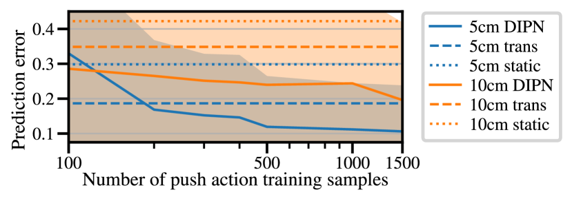
Figure 4: DIPN learning curve with standard deviation visualized as colored areas. The $x$-axis is the number of pushes for training DIPN. The $y$-axis is the prediction error: $1-\text{IoU}$. The dotted and dashed lines are baselines.

Fig. 5 shows typical predictions by DIPN. The network is learned in simulation with randomly shaped and colored objects, and directly transferred to the real system. We observe that DIPN can accurately predict the state after a push, with good accuracy on object orientation and translation.

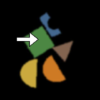
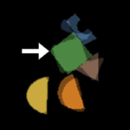
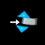
Figure 5: Typical DIPN results. The figures from left to right are: original and predicted images in simulation, and original and predicted images in a real experiment. The ground truth images after a push are overlaid on the predicted images with transparency. The arrows visualize the push actions.

Figure 6: Manually generated hard instances largely similar to the ones in [1]. The cases are used in both simulation and real experiment.

V-B Grasp Network (GN)

We train and evaluate GN as a standalone module and compare it with the state-of-the-art DQN-based method known as Visual Pushing and Grasping (VPG) [1], which learns both grasp and push at the same time. Since GN is only trained on grasp actions, and for a fair comparison, we also tested a third method that learns both grasp and push actions: this method, denoted by DQN+GN, uses GN for learning grasp actions and the DQN structure of [1] to learn push actions. The algorithms are compared using the grasp success rate metric, i.e., the number of objects removed divided by the total number of grasps. We train all algorithms directly on randomly generated PaG instances with $10$ objects.

The learning curve in simulation is provided in Fig. 7. The pre-training process (Alg. 1, line 1, which is also self-supervised) for GN takes $100$ offline images that are not reported in the plot. Comparing DQN+GN which reaches $>90\%$ success rate with less than $300$ (grasp and push) samples, and baseline VPG, which converges at $~{}82\%$ success rate with more than $2000$ (grasp and push) samples, it is clear that GN has significantly higher grasp success rate and sample efficiency than the baseline VPG. As shown by the comparison between GN and DQN+GN, when training using only grasp actions, GN can be more sample efficient without sacrificing success rate. The result also indicates that for randomly generated PaG, pushing is mostly unnecessary.

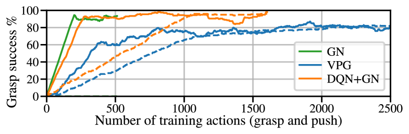
Figure 7: Grasp learning curves of algorithms for PaG in simulation. The $x$-axis is the total number of training steps, i.e., number of actions taken, including push and grasp. The $y$-axis is the grasp success rate. The dashed lines denote the success rate for a grasp right after a push action.

V-C Evaluation of the Complete Pipeline

We evaluate the learned policies on PaG with up to $30$ objects, first in a simulation, then on a real system. Four algorithms are tested: VPG [1], DQN+GN, REA+DIPN, and DIPN+GN (our full pipeline). Here, REA+DIPN follows Alg. 2 but uses the reactive grasp network from [1] instead of GN for grasp reward estimation. We use three metrics for comparison: (i) Completion, calculated as the number of PaG instances where all objects got removed divided by the total number of instances; incomplete tasks are normally due to pushing objects out of the workspace, or cannot finish a task within a number of actions less than three times the number of objects. (ii) Grasp success, calculated as the total number of objects grasped divided by the the total number of grasp actions. (iii) Action efficiency, calculated as the total number of objects removed divided by the total number of actions (grasp and push). For grasp success rate and action efficiency, we use two formulations: one does not count incomplete tasks (reported in gray text), which is the same as the one used in [1], and the other one counts incomplete tasks, which we believe is more reflective. The robot could grasp more than one object at a time. We consider it as a successful grasp, as the goal is to clear all objects from the table.

Table. I reports simulation results on $30$ randomly generated PaG instances and $10$ manually placed hard instances (illustrated in Fig. 6) where push actions are necessary. The algorithms do not see the hard instances in training. The number of training samples for each algorithm are: $2500$ actions (grasp and push) for VPG [1], $1500$ grasp actions and $2000$ push actions for REA+DIPN, $1500$ actions (grasp and push) for DQN+GN, and $500$ grasp actions and $1500$ push actions for DIPN+GN (our full pipeline). The results show that DIPN and GN both are sample efficient in comparison with the baseline and provide significant improvement in PaG metrics; when combined, DIPN+GN reaches the highest performance on all metrics.

TABLE I: Simulation, random and hard instances (mean $\%$)

	Method	Completion	Grasp success		Action efficiency
Rand	VPG[1]	20.0	69.0	52.6	66.3	52.6
	REA[1]+DIPN	83.3	79.5	77.9	77.4	76.3
	DQN[1]+GN	46.7	85.2	83.9	83.4	81.7
	DIPN+GN	83.3	86.7	85.2	84.4	83.3
Hard	VPG[1]	77.7	67.4	60.0	60.8	57.6
	REA[1]+DIPN	90.3	81.5	76.6	64.7	62.6
	DQN[1]+GN	86.0	91.1	87.1	70.2	67.9
	DIPN+GN	100.0	93.3	93.3	74.4	74.4

We repeated the evaluation on a real system (see Fig. 1a). Each random instance contains $10$ randomly selected objects; the hard instances are shown in Fig. 6. Fig. 8 shows grasp learning curve. We compare VPG [1] (trained with $2000$ grasp and push actions) and the proposed DIPN+GN pipeline (pre-trained with $100$ unlabeled RGB-D images for segmentation, trained GN with $500$ grasp actions and DIPN with $1500$ simulated push actions). The evaluation result is reported in Table. II. Remarkably, our networks, while being developed using only simulation based training, perform even better when trained/evaluated only on real hardware.

Figure 8: Grasp learning curves for PaG in real experiment. Solid lines indicate grasp success rate and dotted lines indicate push-then-grasp success rates over training steps. The GN is trained in a grasp only manner.

TABLE II: Real system, random and hard instances (mean $\%$)

	Method	Completion	Grasp success		Action efficiency
Rand	VPG[1]	80.0	85.5	79	75.3	67.9
	DIPN+GN	100.0	94.0	94.0	98.2	98.2
Hard	VPG[1]	64.0	75.1	69.0	51.9	47.8
	DIPN+GN	98.0	89.9	89.9	77.6	78.2

With DIPN and GN outperforming the corresponding components from VPG [1], it is unsurprising that DIPN+GN does much better. In particular, DIPN architecture allows it to learn intelligent, graded push behavior efficiently. In contrast, VPG [1] has a fixed $0.5$ push reward, which sometimes negatively impacts the performance: VPG could push unnecessarily for many times without a grasp when it is not confident enough to grasp. It also risks pushing objects outside of the workspace. Similar to [1], we also tested DIPN+GN with unseen objects, including soapboxes and plastic bottles. Our method obtained similar performance as reported in Table II.

VI Conclusion

In this work, we have developed a Deep Interaction Prediction Network (DIPN) for learning to predict the complex interactions that occur as a robot manipulator pushes objects in clutter. Unlike most existing end-to-end techniques, DIPN is capable of generating accurate predictions in the form of clearly legible synthetic images that can be fed as inputs to a deep Grasp Network (GN), which can then predict successes of future grasps. We demonstrated that DIPN, GN, and DIPN+GN all have excellent sample efficiency and significantly outperform the previous state-of-the-art learning-based method for PaG challenges, while using only a fraction of the interaction data used by the alternative. Our networks are trained in a fully self-supervised manner, without any manual labeling or human inputs, and exhibit high levels of generalizability. The proposed system was initially developed for a simulator, but it surprisingly performed better when trained directly on real hardware and objects. DIPN+GN is also highly robust with respect to changes in objects’ physical properties, such as shape, size, color, and friction. In a future work, we will consider more complex manipulation actions, such as non-horizontal push actions and non-vertical grasps with arbitrary 6D end-effector poses, which are necessary for manipulating everyday objects in clutter.

References

- [1] A. Zeng, S. Song, S. Welker, J. Lee, A. Rodriguez, and T. Funkhouser, “Learning synergies between pushing and grasping with self-supervised deep reinforcement learning,” in 2018 IEEE/RSJ International Conference on Intelligent Robots and Systems (IROS). IEEE, 2018, pp. 4238–4245.
- [2] J. Bohg, A. Morales, T. Asfour, and D. Kragic, “Data-driven grasp synthesis—a survey,” Trans. Rob., vol. 30, no. 2, p. 289–309, Apr. 2014.
- [3] A. Bicchi and V. Kumar, “Robotic grasping and contact: A review.” Proceedings - IEEE International Conference on Robotics and Automation 1, 2000.
- [4] H. Liang, X. Ma, S. Li, M. Görner, S. Tang, B. Fang, F. Sun, and J. Zhang, “PointNetGPD: Detecting grasp configurations from point sets,” in IEEE International Conference on Robotics and Automation (ICRA), 2019.
- [5] A. Rodriguez, M. T. Mason, and S. Ferry, “From caging to grasping,” The International Journal of Robotics Research, vol. 31, no. 7, pp. 886–900, 2012.
- [6] R. Detry, C. H. Ek, M. Madry, and D. Kragic, “Learning a dictionary of prototypical grasp-predicting parts from grasping experience,” 05 2013.
- [7] I. Lenz, H. Lee, and A. Saxena, “Deep learning for detecting robotic grasps,” International Journal of Robotics Research, vol. 34, 01 2013.
- [8] D. Kappler, J. Bohg, and S. Schaal, “Leveraging big data for grasp planning,” in 2015 IEEE International Conference on Robotics and Automation (ICRA), 2015, pp. 4304–4311.
- [9] X. Yan, J. Hsu, M. Khansari, Y. Bai, A. Pathak, A. Gupta, J. Davidson, and H. Lee, “Learning 6-dof grasping interaction via deep 3d geometry-aware representations,” in Proceedings of IEEE International Conference on Robotics and Automation (ICRA 2018), May 2018.
- [10] A. Mousavian, C. Eppner, and D. Fox, “6-dof graspnet: Variational grasp generation for object manipulation,” in 2019 IEEE/CVF International Conference on Computer Vision, ICCV 2019, Seoul, Korea (South), October 27 - November 2, 2019. IEEE, 2019, pp. 2901–2910. [Online]. Available: https://doi.org/10.1109/ICCV.2019.00299
- [11] A. T. Pas and R. Platt, “Using geometry to detect grasp poses in 3d point clouds,” in ISRR, 2015.
- [12] L. Pinto and A. Gupta, “Supersizing self-supervision: Learning to grasp from 50k tries and 700 robot hours,” in 2016 IEEE International Conference on Robotics and Automation, ICRA 2016, Stockholm, Sweden, May 16-21, 2016, D. Kragic, A. Bicchi, and A. D. Luca, Eds. IEEE, 2016, pp. 3406–3413. [Online]. Available: https://doi.org/10.1109/ICRA.2016.7487517
- [13] J. Mahler and K. Goldberg, “Learning deep policies for robot bin picking by simulating robust grasping sequences,” ser. Proceedings of Machine Learning Research, S. Levine, V. Vanhoucke, and K. Goldberg, Eds., vol. 78. PMLR, 13–15 Nov 2017, pp. 515–524.
- [14] J. Mahler, J. Liang, S. Niyaz, M. Laskey, R. Doan, X. Liu, J. A. Ojea, and K. Goldberg, “Dex-net 2.0: Deep learning to plan robust grasps with synthetic point clouds and analytic grasp metrics,” 2017.
- [15] D. Kalashnikov, A. Irpan, P. Pastor, J. Ibarz, A. Herzog, E. Jang, D. Quillen, E. Holly, M. Kalakrishnan, V. Vanhoucke, and S. Levine, “Qt-opt: Scalable deep reinforcement learning for vision-based robotic manipulation,” 2018.
- [16] J. Stüber, C. Zito, and R. Stolkin, “Let’s push things forward: A survey on robot pushing,” Frontiers in Robotics and AI, vol. 7, p. 8, 2020.
- [17] K. Lynch, “Estimating the friction parameters of pushed objects,” in Proceedings of (IROS) IEEE/RSJ International Conference on Intelligent Robots and Systems, vol. 1, July 1993, pp. 186 – 193.
- [18] M. T. Mason, “Mechanics and planning of manipulator pushing operations,” The International Journal of Robotics Research, vol. 5, no. 3, pp. 53–71, 1986.
- [19] K. M. Lynch and M. T. Mason, “Stable pushing: Mechanics, controllability, and planning,” The International Journal of Robotics Research, vol. 15, no. 6, pp. 533–556, 1996.
- [20] ——, “Dynamic nonprehensile manipulation: Controllability, planning, and experiments,” The International Journal of Robotics Research, vol. 18, no. 1, pp. 64–92, 1999.
- [21] S. Akella and M. T. Mason, “Posing polygonal objects in the plane by pushing,” The International Journal of Robotics Research, vol. 17, no. 1, pp. 70–88, 1998.
- [22] M. T. Mason, “On the scope of quasi-static pushing,” in Proceedings of 3rd International Symposium on Robotics Research. Cambridge, Mass: MIT Press, October 1985, pp. 229–233.
- [23] R. D. Howe and M. R. Cutkosky, “Practical force-motion models for sliding manipulation,” The International Journal of Robotics Research, vol. 15, no. 6, pp. 557–572, 1996.
- [24] J. Zhou, R. Paolini, J. A. Bagnell, and M. T. Mason, “A Convex Polynomial Force-Motion Model for Planar Sliding: Identification and Application,” 2 2016. [Online]. Available: https://kilthub.cmu.edu/articles/journal˙contribution/A˙Convex˙Polynomial˙Force-Motion˙Model˙for˙Planar˙Sliding˙Identification˙and˙Application/6550115
- [25] J. Zhou, M. T. Mason, R. Paolini, and D. Bagnell, “A convex polynomial model for planar sliding mechanics: theory, application, and experimental validation,” The International Journal of Robotics Research, vol. 37, no. 2-3, pp. 249–265, 2018.
- [26] J. Zhou, Y. Hou, and M. T. Mason, “Pushing revisited: Differential flatness, trajectory planning, and stabilization,” I. J. Robotics Res., vol. 38, no. 12-13, 2019.
- [27] S. D. Han, N. M. Stiffler, A. Krontiris, K. E. Bekris, and J. Yu, “Complexity results and fast methods for optimal tabletop rearrangement with overhand grasps,” The International Journal of Robotics Research, vol. 37, no. 13-14, pp. 1775–1795, 2018.
- [28] M. R. Dogar and S. S. Srinivasa, “A framework for push-grasping in clutter,” in Robotics: Science and Systems VII, University of Southern California, Los Angeles, CA, USA, June 27-30, 2011, H. F. Durrant-Whyte, N. Roy, and P. Abbeel, Eds., 2011. [Online]. Available: http://www.roboticsproceedings.org/rss07/p09.html
- [29] M. Bauzá and A. Rodriguez, “A probabilistic data-driven model for planar pushing,” in 2017 IEEE International Conference on Robotics and Automation, ICRA 2017, Singapore, Singapore, May 29 - June 3, 2017. IEEE, 2017, pp. 3008–3015.
- [30] C. Finn, I. Goodfellow, and S. Levine, “Unsupervised learning for physical interaction through video prediction,” in Advances in neural information processing systems, 2016, pp. 64–72.
- [31] A. Byravan and D. Fox, “Se3-nets: Learning rigid body motion using deep neural networks,” in 2017 IEEE International Conference on Robotics and Automation (ICRA), 2017, pp. 173–180.
- [32] N. Watters, D. Zoran, T. Weber, P. Battaglia, R. Pascanu, and A. Tacchetti, “Visual interaction networks: Learning a physics simulator from video,” in Advances in neural information processing systems, 2017, pp. 4539–4547.
- [33] M. Szegedy and J. Yu, “On rearrangement of items stored in stacks,” arXiv preprint arXiv:2002.04979, 2020.
- [34] R. Shome, K. Solovey, J. Yu, K. Bekris, and D. Halperin, “Fast, high-quality two-arm rearrangement in synchronous, monotone tabletop setups,” IEEE Transactions on Automation Science and Engineering, 2021.
- [35] L. Sergey, N. Wagener, and P. Abbeel, “Learning contact-rich manipulation skills with guided policy search,” in Proceedings of the 2015 IEEE International Conference on Robotics and Automation (ICRA), Seattle, WA, USA, 2015, pp. 26–30.
- [36] S. Levine, C. Finn, T. Darrell, and P. Abbeel, “End-to-end training of deep visuomotor policies,” J. Mach. Learn. Res., vol. 17, no. 1, p. 1334–1373, Jan. 2016.
- [37] C. Finn and S. Levine, “Deep visual foresight for planning robot motion,” in 2017 IEEE International Conference on Robotics and Automation, ICRA 2017, Singapore, Singapore, May 29 - June 3, 2017. IEEE, 2017, pp. 2786–2793. [Online]. Available: https://doi.org/10.1109/ICRA.2017.7989324
- [38] A. Ghadirzadeh, A. Maki, D. Kragic, and M. Björkman, “Deep predictive policy training using reinforcement learning,” CoRR, vol. abs/1703.00727, 2017. [Online]. Available: http://arxiv.org/abs/1703.00727
- [39] C. Song and A. Boularias, “Object rearrangement with nested nonprehensile manipulation actions,” in IEEE International Conference on Intelligent Robots and Systems, IROS, Macau, China, 2019.
- [40] R. Shome, W. Tang, C. Song, C. Mitash, C. Kourtev, J. Yu, A. Boularias, and K. Bekris, “Towards robust product packing with a minimalistic end-effector,” in IEEE International Conference on Robotics and Automation, ICRA 2019, Montreal, Canada, May 2019, 2019.
- [41] K. Hang, A. Morgan, and A. Dollar, “Pre-grasp sliding manipulation of thin objects using soft, compliant, or underactuated hands,” IEEE Robotics and Automation Letters, vol. PP, pp. 1–1, 01 2019.
- [42] M. R. Dogar and S. S. Srinivasa, “Push-grasping with dexterous hands: Mechanics and a method,” 2010 IEEE/RSJ International Conference on Intelligent Robots and Systems, pp. 2123–2130, 2010.
- [43] M. R. Dogar, M. C. Koval, A. Tallavajhula, and S. S. Srinivasa, “Object search by manipulation,” in 2013 IEEE International Conference on Robotics and Automation, May 2013, pp. 4973–4980.
- [44] M. Dogar, K. Hsiao, M. Ciocarlie, and S. Srinivasa, “Physics-Based Grasp Planning Through Clutter,” in R:SS, July 2012.
- [45] J. E. King, M. Klingensmith, C. M. Dellin, M. R. Dogar, P. Velagapudi, N. S. Pollard, and S. S. Srinivasa, “Pregrasp manipulation as trajectory optimization,” in Robotics: Science and Systems, 2013.
- [46] A. Boularias, O. Kroemer, and J. Peters, “Learning robot grasping from 3-d images with markov random fields,” in 2011 IEEE/RSJ International Conference on Intelligent Robots and Systems, IROS 2011, San Francisco, CA, USA, September 25-30, 2011, 2011, pp. 1548–1553. [Online]. Available: http://dx.doi.org/10.1109/IROS.2011.6094888
- [47] A. Boularias, J. A. Bagnell, and A. Stentz, “Efficient optimization for autonomous robotic manipulation of natural objects,” in Proceedings of the Twenty-Eighth AAAI Conference on Artificial Intelligence, July 27 -31, 2014, Québec City, Québec, Canada., 2014, pp. 2520–2526. [Online]. Available: http://www.aaai.org/ocs/index.php/AAAI/AAAI14/paper/view/8414
- [48] T. Yoshikawa and M. Kurisu, “Indentification of the center of friction from pushing an object by a mobile robot,” Proceedings IROS ’91:IEEE/RSJ International Workshop on Intelligent Robots and Systems ’91, pp. 449–454 vol.2, 1991.
- [49] C. Song and A. Boularias, “Learning to slide unknown objects with differentiable physics simulations,” in Proceedings of Robotics: Science and Systems (RSS) , Corvallis, Oregon, 2020, 2020.
- [50] ——, “A probabilistic model for planar sliding of objects with unknown material properties: Identification and robust planning,” in IEEE/RSJ International Conference on Intelligent Robots and Systems, IROS 2020, Las Vegas, NV, USA, October 24, 2020 - January 24, 2021. IEEE, 2020, pp. 5311–5318. [Online]. Available: https://doi.org/10.1109/IROS45743.2020.9341468
- [51] ——, “Identifying mechanical models of unknown objects with differentiable physics simulations,” in Proceedings of the 2020 Learning for Dynamics and Control Conference (L4DC), Berkeley, California, 2020, 2020.
- [52] A. Boularias, J. A. Bagnell, and A. Stentz, “Learning to manipulate unknown objects in clutter by reinforcement,” in Proceedings of the Twenty-Ninth AAAI Conference on Artificial Intelligence, January 25-30, 2015, Austin, Texas, USA., 2015, pp. 1336–1342. [Online]. Available: http://www.aaai.org/ocs/index.php/AAAI/AAAI15/paper/view/9360
- [53] K. He, G. Gkioxari, P. Dollár, and R. Girshick, “Mask r-cnn,” in Proceedings of the IEEE international conference on computer vision, 2017, pp. 2961–2969.
- [54] T. Lin, P. Dollár, R. B. Girshick, K. He, B. Hariharan, and S. J. Belongie, “Feature pyramid networks for object detection,” CoRR, vol. abs/1612.03144, 2016. [Online]. Available: http://arxiv.org/abs/1612.03144
- [55] L. Yen-Chen, A. Zeng, S. Song, P. Isola, and T.-Y. Lin, “Learning to see before learning to act: Visual pre-training for manipulation,” in 2020 IEEE International Conference on Robotics and Automation (ICRA). IEEE, 2020, pp. 7286–7293.
- [56] E. Rohmer, S. P. Singh, and M. Freese, “V-rep: A versatile and scalable robot simulation framework,” in 2013 IEEE/RSJ International Conference on Intelligent Robots and Systems. IEEE, 2013, pp. 1321–1326.