Abstract

We consider optimal control of an unknown multi-agent linear quadratic (LQ) system where the dynamics and the cost are coupled across the agents through the mean-field (i.e., empirical mean) of the states and controls. Directly using single-agent LQ learning algorithms in such models results in regret which increases polynomially with the number of agents. We propose a new Thompson sampling based learning algorithm which exploits the structure of the system model and show that the expected Bayesian regret of our proposed algorithm for a system with agents of $|M|$ different types at time horizon $T$ is $\tilde{\mathcal{O}}\big{(}|M|^{1.5}\sqrt{T}\big{)}$ irrespective of the total number of agents, where the $\tilde{\mathcal{O}}$ notation hides logarithmic factors in $T$. We present detailed numerical experiments to illustrate the salient features of the proposed algorithm.

1 Introduction

Linear dynamical systems with a quadratic cost (henceforth referred to as LQ systems) are one of the most commonly used modeling framework in robotics, aerospace, electrical circuits, mechanical systems, thermodynamical systems, and chemical and industrial plants. Part of the appeal of LQ models is that the optimal control action in such models is a linear or affine function of the state; therefore, the optimal policy is easy to identify and easy to implement.

Broadly speaking, three classes of learning algorithms have been proposed for LQ systems: Optimism in the face of uncertainty (OFU) based algorithms, certainty equivalence (CE) based algorithms, and Thompson sampling (TS) based algorithms.

OFU-based algorithms are inspired by the OFU principle for multi-armed bandits (Auer et al., 2002). Starting with the work of (Campi and Kumar, 1998; Abbasi-Yadkori and Szepesvári, 2011), most of the papers following this approach (Faradonbeh et al., 2017; Cohen et al., 2019; Abeille and Lazaric, 2020) provide a high probability bound on regret. As an illustrative example, it is shown in (Abeille and Lazaric, 2020) that, with high probability, the regret of a OFU-based learning algorithm is $\tilde{\mathcal{O}}(d_{x}^{0.5}(d_{x}+d_{u})\sqrt{T})$, where $d_{x}$ is the dimension of the state, $d_{u}$ is the dimension of the controls, $T$ is the time horizon, and the $\tilde{\mathcal{O}}(\cdot)$ notation hides logarithmic terms in $T$.

Certainty equivalence (CE) is a classical adaptive control algorithm in Systems and Control (Astrom and Wittenmark, 1994). Most papers following this approach (Dean et al., 2018; Mania et al., 2019; Faradonbeh et al., 2020; Simchowitz and Foster, 2020) also provide a high probability bound on regret. As an illustrative example, it is shown in (Simchowitz and Foster, 2020) that, with high probability, the regret of a CE-based algorithm is $\tilde{\mathcal{O}}(d_{x}^{0.5}d_{u}\sqrt{T}+d_{x}^{2})$.

Thompson sampling (TS) based algorithms are inspired by TS algorithm for multi-armed bandits (Agrawal and Goyal, 2012). Most papers following this approach (Ouyang et al., 2017, 2019; Abeille and Lazaric, 2018) establish a bound on the expected Bayesian regret. As an illustrative example, (Ouyang et al., 2019) shows that the regret of a TS-based algorithm is $\tilde{\mathcal{O}}(d_{x}^{0.5}(d_{x}+d_{u})\sqrt{T})$.

Two aspects of these regret bounds are important: the dependence on the time horizon $T$ and the dependence on the dimensions $(d_{x},d_{u})$ of the state and the controls. For all classes of algorithms mentioned above, the dependence on the time horizon is $\tilde{\mathcal{O}}(\sqrt{T})$. Moreover, there are multiple papers which show that, under different assumptions, the regret is lower bounded by $\Omega(\sqrt{T})$ (Cassel et al., 2020; Simchowitz and Foster, 2020). So, the time dependence in the available regret bounds is nearly order optimal. Similarly, even though the dependence of the regret bound on the dimensions of the state and the control varies slightly for each class of algorithms, Simchowitz and Foster (2020) recently showed that the regret is lower bounded by $\tilde{\Omega}(d_{x}^{0.5}d_{u}\sqrt{T})$. So, there is only a small scope of improvement in the dimension dependence in the regret bounds.

The dependence of the regret bounds on the dimensions of the state and controls is critical for applications such as formation control of robotic swarms and demand response in power grids which have large numbers of agents (which can be of the order of $10^{3}$ to $10^{5}$). In such systems, the effective dimension of the state and the controls is $nd_{x}$ and $nd_{u}$, where $n$ is the number of agents and $d_{x}$ and $d_{u}$ are the dimensions of the state and controls of each agent. Therefore, if we take the regret bound of, say, the OFU algorithm proposed in Abeille and Lazaric (2020), the regret is $\tilde{\mathcal{O}}(n^{1.5}d_{x}^{0.5}({d_{x}+d_{u}})\sqrt{T})$. Similar scaling with $n$ holds for CE- and TS-based algorithms. The polynomial dependence on the number of agents is prohibitive and, because of it, the standard regret bounds are of limited value for large-scale systems.

There are many papers in the planning literature on the design of large-scale systems which exploit some structural property of the system to develop low-complexity design algorithms (Lunze, 1986; Sundareshan and Elbanna, 1991; Yang and Zhang, 1995; Hamilton and Broucke, 2012; Arabneydi and Mahajan, 2015, 2016). However, there has been very little investigation on the role of such structural properties in developing and analyzing learning algorithms.

Our main contribution is to show that by carefully exploiting the structure of the model, it is possible to design learning algorithms for large-scale LQ systems where the regret does not grow polynomially in the number of agents. In particular, we investigate mean-field coupled control systems, which have gained considerable importance in the last 10–15 years (Lasry and Lions, 2007; Huang et al., 2007, 2012; Weintraub et al., 2005, 2008). There is a large literature on different variations of such models and we refer the reader to Gomes et al. (2014) for a survey. There has been considerable interest in reinforcement learning for such models (Yang et al., 2018; Subramanian and Mahajan, 2019; Tiwari et al., 2019; Guo et al., 2019; Subramanian et al., 2020; Zhang et al., 2020), but all of these papers focus on identifying asymptotically optimal policies and do not characterize regret.

Our main contribution is to design a TS-based algorithm for mean-field teams (which is a specific mean-field model proposed in Arabneydi and Mahajan (2015, 2016)) and show that (for a system with homogeneous agents) the regret scales as $\tilde{\mathcal{O}}(|M|^{1.5}d_{x}^{0.5}(d_{x}+d_{u})\sqrt{T})$, where $|M|$ is the number of types.

We would like to highlight that although we focus on a TS-based algorithm in the paper, it will be clear from the derivation that it is possible to develop OFU- and CE-based algorithms with similar regret bounds. Thus, the main takeaway message of our paper is that there is significant value in developing learning algorithms which exploit the structure of the model.

2 Background on mean-field teams

2.1 Mean-field teams model

We start by describing a slight generalization of the basic model of mean-field teams proposed in Arabneydi and Mahajan (2015, 2016).

Consider a system with a large population of agents. The agents are heterogeneous and have multiple types. Let $M=\{1,\dots,\lvert M\rvert\}$ denote the set of types of agents, $N^{m}$, $m\in M$, denote the set of all agents of type $m$, and $N=\bigcup_{m\in M}N^{m}$ denote the set of all agents.

States, actions, and their mean-fields:

Agents of the same type have the same state and action spaces. In particular, the state and control action of agents of type $m$ take values in $\mathds{R}^{d^{m}_{x}}$ and $\mathds{R}^{d^{m}_{u}}$, respectively. For any generic agent $i\in N^{m}$ of type $m$, we use $x^{i}_{t}\in\mathds{R}^{d^{m}_{x}}$ and $u^{i}_{t}\in\mathds{R}^{d^{m}_{u}}$ to denote its state and control action at time $t$. We use $\bm{x}_{t}=\operatorname{vec}((x^{i}_{t})_{i\in N})$ and $\bm{u}_{t}=\operatorname{vec}((u^{i}_{t})_{i\in N})$ to denote the global state and control actions of the system at time $t$.

The empirical mean-field $(\bar{x}^{m}_{t},\bar{u}^{m}_{t})$ of agents of type $m$, $m\in M$, is defined as the empirical mean of the states and actions of all agents of that type, i.e.,

$$\bar{x}^{m}_{t}=\frac{1}{\lvert N^{m}\rvert}\sum_{i\in N^{m}}x^{i}_{t}\quad\text{and}\quad\bar{u}^{m}_{t}=\frac{1}{\lvert N^{m}\rvert}\sum_{i\in N^{m}}u^{i}_{t}.$$

The empirical mean-field $(\bm{\bar{x}}_{t},\bm{\bar{u}}_{t})$ of the entire population is given by

$$\bm{\bar{x}}_{t}=\operatorname{vec}(\bar{x}_{t}^{1},\dots,\bar{x}_{t}^{|M|})\quad\text{and}\quad\bm{\bar{u}}_{t}=\operatorname{vec}(\bar{u}_{t}^{1},\dots,\bar{u}_{t}^{|M|}).$$

As an example, consider the temperature control of a multi-storied office building. In this case, $N$ represents the set of rooms, $M$ represents the set of floors, $N^{m}$ represents all rooms in floor $m$, $x^{i}_{t}$ represents the temperature in room $i$, $\bar{x}^{m}_{t}$ represents the average temperature in floor $m$, and $\bm{\bar{x}}_{t}$ represents the collection of average temperature in each floor. Similarly, $u^{i}_{t}$ represents the heat exchanged by the air-conditioner in room $i$, $\bar{u}^{m}_{t}$ represents the average heat exchanged by the air-conditioners in floor $m$, and $\bm{\bar{u}}_{t}$ represents the collection of average heat exchanged in each floor of the building.

System dynamics and per-step cost:

The system starts at a random initial state $x_{1}=(x^{i}_{1})_{i\in N}$, whose components are independent across agents. For agent $i$ of type $m$, the initial state $x^{i}_{1}\sim\mathcal{N}(0,\mathsf{X}^{i}_{1})$, and at time $t\geq 1$, the state evolves according to

$$x^{i}_{t+1}=\mathsf{A}^{m}x^{i}_{t}+\mathsf{B}^{m}u^{i}_{t}+\mathsf{D}^{m}\bm{\bar{x}}_{t}+\mathsf{E}^{m}\bm{\bar{u}}_{t}+w^{i}_{t}+v^{m}_{t}+\mathsf{F}^{m}v^{0}_{t},$$ (1)

where $\mathsf{A}^{m}$, $\mathsf{B}^{m}$, $\mathsf{D}^{m}$, $\mathsf{E}^{m}$, $\mathsf{F}^{m}$ are matrices of appropriate dimensions, $\{w^{i}_{t}\}_{t\geq 1}$, $\{v^{m}_{t}\}_{t\geq 1}$, and $\{v^{0}_{t}\}_{t\geq 1}$ are i.i.d. zero-mean Gaussian processes which are independent of each other and the initial state. In particular, $w^{i}_{t}\in\mathds{R}^{d^{m}_{x}}$, $v^{m}_{t}\in\mathds{R}^{d^{m}_{x}}$, and $v^{0}_{t}\in\mathds{R}^{d^{0}_{v}}$, and $w^{i}_{t}\sim\mathcal{N}(0,\mathsf{W}^{i})$, $v^{m}_{t}\sim\mathcal{N}(0,\mathsf{V}^{m})$, and $v^{0}_{t}\sim\mathcal{N}(0,\mathsf{V}^{0})$.

Eq. (1) implies that all agents of type $m$ have similar dynamical couplings. The next state of agent $i$ of type $m$ depends on its current local state and control action, the current mean-field of the states and control actions of the system, and is influenced by three independent noise processes: a local noise process $\{w^{i}_{t}\}_{t\geq 1}$, a noise process $\{v^{m}_{t}\}_{t\geq 1}$ which is common to all agents of type $m$, and a global noise process $\{v^{0}_{t}\}_{t\geq 1}$ which is common to all agents.

At each time-step, the system incurs a quadratic cost $c(\bm{x}_{t},\bm{u}_{t})$ given by

$$c(\bm{x}_{t},\bm{u}_{t})=\bm{\bar{x}}_{t}^{\mathchoice{\raisebox{0.0pt}{$\displaystyle\intercal$}}{\raisebox{0.0pt}{$\textstyle\intercal$}}{\raisebox{0.0pt}{$\scriptstyle\intercal$}}{\raisebox{0.0pt}{$\scriptscriptstyle\intercal$}}}\bar{\mathsf{Q}}\bm{\bar{x}}_{t}+\bm{\bar{u}}_{t}^{\mathchoice{\raisebox{0.0pt}{$\displaystyle\intercal$}}{\raisebox{0.0pt}{$\textstyle\intercal$}}{\raisebox{0.0pt}{$\scriptstyle\intercal$}}{\raisebox{0.0pt}{$\scriptscriptstyle\intercal$}}}\bar{\mathsf{R}}\bm{\bar{u}}_{t}\\ +\sum_{m\in M}\frac{1}{\lvert N^{m}\rvert}\sum_{i\in N^{m}}\bigl{[}(x^{i}_{t})^{\mathchoice{\raisebox{0.0pt}{$\displaystyle\intercal$}}{\raisebox{0.0pt}{$\textstyle\intercal$}}{\raisebox{0.0pt}{$\scriptstyle\intercal$}}{\raisebox{0.0pt}{$\scriptscriptstyle\intercal$}}}\mathsf{Q}^{m}x^{i}_{t}+(u^{i}_{t})^{\mathchoice{\raisebox{0.0pt}{$\displaystyle\intercal$}}{\raisebox{0.0pt}{$\textstyle\intercal$}}{\raisebox{0.0pt}{$\scriptstyle\intercal$}}{\raisebox{0.0pt}{$\scriptscriptstyle\intercal$}}}\mathsf{R}^{m}u^{i}_{t}\bigr{]}.$$ (2)

Thus, there is a weak coupling in the cost of the agents through the mean-field.

Admissible policies and performance criterion:

There is a system operator who has access to the states of all agents and control actions and chooses the control action according to a deterministic or randomized policy

$$\bm{u}_{t}=\pi_{t}(\bm{x}_{1:t},\bm{u}_{1:t-1}).$$ (3)

Let $\bm{\theta}=(\theta^{m})_{m\in M}$, where $(\theta^{m})^{\mathchoice{\raisebox{0.0pt}{$\displaystyle\intercal$}}{\raisebox{0.0pt}{$\textstyle\intercal$}}{\raisebox{0.0pt}{$\scriptstyle\intercal$}}{\raisebox{0.0pt}{$\scriptscriptstyle\intercal$}}}=[\mathsf{A}^{m},\mathsf{B}^{m},\mathsf{D}^{m},\mathsf{E}^{m},\mathsf{F}^{m}]$, denotes the parameters of the system dynamics. The performance of any policy $\pi=(\pi_{1},\pi_{2},\dots)$ is given by

$$J(\pi;\bm{\theta})=\limsup_{T\to\infty}\frac{1}{T}\mathbb{E}\Bigl{[}\sum_{t=1}^{T}c(\bm{x}_{t},\bm{u}_{t})\Bigr{]}.$$ (4)

Let $J(\bm{\theta})$ to denote the minimum of $J(\pi;\bm{\theta})$ over all policies.

We are interested in the setup where the system dynamics $\bm{\theta}$ are unknown and there is a prior $p$ on $\bm{\theta}$. The Bayesian regret of a policy $\pi$ operating for a horizon $T$ is defined as

$$R(T;\pi)\coloneqq\mathbb{E}^{\pi}\biggl{[}\sum_{t=1}^{T}c(\bm{x}_{t},\bm{u}_{t})-TJ(\bm{\theta})\biggr{]}$$ (5)

where the expectation is with respect to the prior on $\theta$, the noise processes, the initial conditions, and the potential randomizations done by the policy $\pi$.

2.2 Planning solution for mean-field teams

In this section, we summarize the planning solution of mean-field teams presented in Arabneydi and Mahajan (2015, 2016) for a known system model.

Define the following matrices:

$$\bar{\mathsf{A}} =\operatorname{diag}(\mathsf{A}^{1},\dots,\mathsf{A}^{|M|})+\operatorname{rows}(\mathsf{D}^{1},\dots,\mathsf{D}^{|M|}),$$

$$\bar{\mathsf{B}} =\operatorname{diag}(\mathsf{B}^{1},\dots,\mathsf{B}^{|M|})+\operatorname{rows}(\mathsf{E}^{1},\dots,\mathsf{E}^{|M|}),$$

and let $\bar{\bar{\mathsf{Q}}}=\operatorname{diag}(\mathsf{Q}^{1},\dots,\mathsf{Q}^{|M|})+\bar{\mathsf{Q}}$ and $\bar{\bar{\mathsf{R}}}=\operatorname{diag}(\mathsf{R}^{1},\dots,\mathsf{R}^{|M|})+\bar{\mathsf{R}}$.

It is assumed that the system satisfies the following:

(A1)

$\bar{\bar{\mathsf{Q}}}>0$ and $\bar{\bar{\mathsf{R}}}>0$. Moreover, for every $m\in M$, $\mathsf{Q}^{m}>0$ and $\mathsf{R}^{m}>0$.

(A2)

The system $(\bar{\mathsf{A}},\bar{\mathsf{B}})$ is stabilizable. Moreover, for every $m\in M$, the system $(\mathsf{A}^{m},\mathsf{B}^{m})$ is stabilizable.

Now, consider the following $|M|+1$ discrete time algebraic Riccati equations (DARE):

$$\breve{\mathsf{S}}^{m} =\operatorname{DARE}(\mathsf{A}^{m},\mathsf{B}^{m}\mathsf{Q}^{m},\mathsf{R}^{m}),\quad m\in M,$$ (6a)

$$\bar{\mathsf{S}} =\operatorname{DARE}(\bar{\mathsf{A}},\bar{\mathsf{B}},\bar{\bar{\mathsf{Q}}},\bar{\bar{\mathsf{R}}}).$$ (6b)

Moreover, define

$$\breve{\mathsf{L}}^{m} =-\bigl{(}(\mathsf{B}^{m})^{\mathchoice{\raisebox{0.0pt}{$\displaystyle\intercal$}}{\raisebox{0.0pt}{$\textstyle\intercal$}}{\raisebox{0.0pt}{$\scriptstyle\intercal$}}{\raisebox{0.0pt}{$\scriptscriptstyle\intercal$}}}\breve{\mathsf{S}}^{m}\mathsf{B}^{m}+\mathsf{R}^{m}\bigr{)}^{-1}(\mathsf{B}^{m})^{\mathchoice{\raisebox{0.0pt}{$\displaystyle\intercal$}}{\raisebox{0.0pt}{$\textstyle\intercal$}}{\raisebox{0.0pt}{$\scriptstyle\intercal$}}{\raisebox{0.0pt}{$\scriptscriptstyle\intercal$}}}\breve{\mathsf{S}}^{m}\mathsf{A}^{m},\quad m\in M,$$ (7a)

$$\bar{\mathsf{L}} =-\bigl{(}\bar{\mathsf{B}}^{\mathchoice{\raisebox{0.0pt}{$\displaystyle\intercal$}}{\raisebox{0.0pt}{$\textstyle\intercal$}}{\raisebox{0.0pt}{$\scriptstyle\intercal$}}{\raisebox{0.0pt}{$\scriptscriptstyle\intercal$}}}\bar{\mathsf{S}}\bar{\mathsf{B}}+\bar{\bar{\mathsf{R}}}\bigr{)}^{-1}\bar{\mathsf{B}}^{\mathchoice{\raisebox{0.0pt}{$\displaystyle\intercal$}}{\raisebox{0.0pt}{$\textstyle\intercal$}}{\raisebox{0.0pt}{$\scriptstyle\intercal$}}{\raisebox{0.0pt}{$\scriptscriptstyle\intercal$}}}\bar{\mathsf{S}}\bar{\mathsf{A}},$$ (7b)

and let $\operatorname{rows}(\bar{\mathsf{L}}^{1},\dots,\bar{\mathsf{L}}^{|M|})=\bar{\mathsf{L}}$.

Finally, define $\bar{w}^{m}_{t}=\frac{1}{\lvert N^{m}\rvert}\sum_{i\in N^{m}}w^{i}_{t}$, $\bm{\bar{w}}_{t}=\operatorname{vec}(\bar{w}_{t}^{1},\dots,\bar{w}_{t}^{|M|})$ and $\bm{\bar{v}}_{t}=\operatorname{vec}(v_{t}^{1},\dots,v_{t}^{|M|})$. Let $\breve{\mathsf{W}}^{m}=\frac{1}{\lvert N^{m}\rvert}\sum_{i\in N^{m}}\operatorname{var}(w^{i}_{t}-\bar{w}^{m}_{t})$ and $\bar{\mathsf{W}}=\operatorname{var}(\bm{\bar{w}}_{t})+\operatorname{diag}(\mathsf{V}^{1},\dots,\mathsf{V}^{|M|})+\operatorname{diag}(\mathsf{F}^{1}\mathsf{V}^{0},\dots,\mathsf{F}^{|M|}\mathsf{V}^{0}).$ Note that since the noise processes are i.i.d., these covariances do not depend on time.

Now, split the state $x^{i}_{t}$ of agent $i$ of type $m$ into two parts: the mean-field state $\bar{x}^{m}_{t}$ and the relative state $\breve{x}^{i}_{t}=x^{i}_{t}-\bar{x}^{m}_{t}$. Do a similar split of the controls: $u^{i}_{t}=\bar{u}^{m}_{t}+\breve{u}^{i}_{t}$. Since $\sum_{i\in N^{m}}\breve{x}^{i}_{t}=0$ and $\sum_{i\in N^{m}}\breve{u}^{i}_{t}=0$, the per-step cost (2) can be written as

$$c(\bm{x}_{t},\bm{u}_{t})=\bar{c}(\bm{\bar{x}}_{t},\bm{\bar{u}}_{t})+\sum_{m\in M}\frac{1}{\lvert N^{m}\rvert}\sum_{i\in N^{m}}\breve{c}^{m}(\breve{x}^{i}_{t},\breve{u}^{i}_{t})$$ (8)

where $\bar{c}(\bm{\bar{x}}_{t},\bm{\bar{u}}_{t})=\bm{\bar{x}}_{t}^{\mathchoice{\raisebox{0.0pt}{$\displaystyle\intercal$}}{\raisebox{0.0pt}{$\textstyle\intercal$}}{\raisebox{0.0pt}{$\scriptstyle\intercal$}}{\raisebox{0.0pt}{$\scriptscriptstyle\intercal$}}}\bar{\bar{\mathsf{Q}}}\bm{\bar{x}}_{t}+\bm{\bar{u}}_{t}^{\mathchoice{\raisebox{0.0pt}{$\displaystyle\intercal$}}{\raisebox{0.0pt}{$\textstyle\intercal$}}{\raisebox{0.0pt}{$\scriptstyle\intercal$}}{\raisebox{0.0pt}{$\scriptscriptstyle\intercal$}}}\bar{\bar{\mathsf{R}}}\bm{\bar{u}}_{t}$ and $\breve{c}^{m}(\breve{x}^{i}_{t},\breve{u}^{i}_{t})=(\breve{x}^{i}_{t})^{\mathchoice{\raisebox{0.0pt}{$\displaystyle\intercal$}}{\raisebox{0.0pt}{$\textstyle\intercal$}}{\raisebox{0.0pt}{$\scriptstyle\intercal$}}{\raisebox{0.0pt}{$\scriptscriptstyle\intercal$}}}\mathsf{Q}^{m}\breve{x}^{i}_{t}+(\breve{u}^{i}_{t})^{\mathchoice{\raisebox{0.0pt}{$\displaystyle\intercal$}}{\raisebox{0.0pt}{$\textstyle\intercal$}}{\raisebox{0.0pt}{$\scriptstyle\intercal$}}{\raisebox{0.0pt}{$\scriptscriptstyle\intercal$}}}\mathsf{R}^{m}\breve{u}^{i}_{t}$. Moreover, the dynamics of mean-field and the relative components of the state are:

$$\bm{\bar{x}}_{t+1}=\bar{\mathsf{A}}\bm{\bar{x}}_{t}+\bar{\mathsf{B}}\bm{\bar{u}}_{t}+\bm{\bar{w}}_{t}+\bm{\bar{v}}_{t}+\bar{\mathsf{F}}v^{0}_{t}$$ (9)

where $\bar{\mathsf{F}}=\operatorname{diag}(\mathsf{F}^{1},\dots,\mathsf{F}^{|M|})$ and for any agent $i$ of type $m$,

$$\breve{x}^{i}_{t}=\mathsf{A}^{m}_{t}\breve{x}^{i}_{t}+\mathsf{B}^{m}\breve{u}^{i}_{t}+\breve{w}^{i}_{t},$$ (10)

where $\breve{w}^{i}_{t}=w^{i}_{t}-\bar{w}^{m}_{t}$.

The result below follows from (Arabneydi and Mahajan, 2016, Theorem 6): Under assumptions (A1) and (A2), the optimal policy for minimizing the cost (4) is given by

$$u^{i}_{t}=\breve{\mathsf{L}}^{m}\breve{x}^{i}_{t}+\bar{\mathsf{L}}^{m}\bm{\bar{x}}_{t}.$$ (11)

Furthermore, the optimal performance is given by

$$J(\bm{\theta})=\sum_{m\in M}\operatorname{Tr}(\breve{\mathsf{W}}^{m}\breve{\mathsf{S}}^{m})+\operatorname{Tr}(\bar{\mathsf{W}}\bar{\mathsf{S}}).$$ (12)

Interpretation of the planning solution:

Note that $\bm{\bar{u}}_{t}=\bar{\mathsf{L}}_{t}\bm{\bar{x}}_{t}$ is the optimal control for the mean-field system with dynamics (9) and per-step cost $\bar{c}(\bm{\bar{x}}_{t},\bm{\bar{u}}_{t})$. Moreover, for agent $i$ of type $m$, $\breve{u}^{i}_{t}=\breve{\mathsf{L}}^{m}_{t}\breve{x}^{i}_{t}$ is the optimal control for the relative system with dynamics (10) and per-step cost $\breve{c}^{m}(\breve{x}^{i}_{t},\breve{u}^{i}_{t})$. Theorem 2.2 shows that at every agent $i$ of type $m$, we can consider the two decoupled systems—the mean-field system and the relative system— solve them separately, and then simply add their respective controls—$\bar{u}^{m}_{t}$ and $\breve{u}^{i}_{t}$—to obtain the optimal control action at agent $i$ in the original mean-field team system. We will exploit this feature of the planning solution in order to develop a learning algorithm for mean-field teams.

3 Learning for mean-field teams

For the ease of exposition, we describe the algorithm for the special case when all types are of the same dimension (i.e., $d^{m}_{x}=d_{x}$ and $d^{m}_{u}=d_{u}$ for all $m\in M$) and the same number of agents (i.e., $|N^{m}|=n$ for all $m\in M$). We further assume that $d^{0}_{v}=d_{x}$ and $\mathsf{F}^{m}=I$. Moreover, we assume noise covariances are given as $\mathsf{W}^{i}=\sigma_{w}^{2}I$, $i\in N$, $\mathsf{V}^{m}=\sigma_{v}^{2}I$, $m\in M$, and $\mathsf{V}^{0}=\sigma_{v^{0}}^{2}I$.

The above assumptions are not strictly needed for the analysis but we impose them because, under these assumptions, the covariance matrices $\bar{\Sigma}$ and $\breve{\Sigma}^{m}$ are scaled identity matrices. In particular, for any $m\in M$, $\breve{\Sigma}^{m}=(1-\frac{1}{n})\sigma_{w}^{2}I\eqqcolon\breve{\sigma}^{2}I$ and $\bar{\Sigma}=(\frac{\sigma_{w}^{2}}{n}+\sigma_{v}^{2}+\sigma_{v^{0}}^{2})I\eqqcolon\bar{\sigma}^{2}I$. This simpler form of the covariance matrices simplifies the description of the algorithm and the regret bounds.

Following the decomposition presented in Sec. 2.2, we define $\bar{\theta}^{\mathchoice{\raisebox{0.0pt}{$\displaystyle\intercal$}}{\raisebox{0.0pt}{$\textstyle\intercal$}}{\raisebox{0.0pt}{$\scriptstyle\intercal$}}{\raisebox{0.0pt}{$\scriptscriptstyle\intercal$}}}=[\bar{\mathsf{A}},\bar{\mathsf{B}}]$ to be the parameters of the mean-field dynamics (9) and $(\breve{\theta}^{m})^{\mathchoice{\raisebox{0.0pt}{$\displaystyle\intercal$}}{\raisebox{0.0pt}{$\textstyle\intercal$}}{\raisebox{0.0pt}{$\scriptstyle\intercal$}}{\raisebox{0.0pt}{$\scriptscriptstyle\intercal$}}}=[\mathsf{A}^{m},\mathsf{B}^{m}]$ to be the parameters of the relative dynamics (10). We let $\breve{\mathsf{S}}^{m}(\breve{\theta}^{m})$ and $\bar{\mathsf{S}}(\bar{\theta})$ denote the solution to the Riccati equations (6) and $\breve{\mathsf{L}}^{m}(\breve{\theta}^{m})$ and $\bar{\mathsf{L}}(\bar{\theta})$ denote the corresponding gains (7). Let $\breve{J}^{m}(\breve{\theta}^{m})=\breve{\sigma}^{2}\operatorname{Tr}(\breve{\mathsf{S}}(\breve{\theta}^{m}))$ and $\bar{J}(\bar{\theta})=\bar{\sigma}^{2}\operatorname{Tr}(\bar{\mathsf{S}}(\bar{\theta}))$ denote the performance of the $m$-th relative system and the mean-field system, respectively. As shown in Theorem 2.2,

$$J(\bm{\theta})=\sum_{m\in M}\breve{J}^{m}(\breve{\theta}^{m})+\bar{J}(\bar{\theta}).$$ (13)

Prior and posterior beliefs:

We assume that the unknown parameters $\breve{\theta}^{m}$, $m\in M$, lie in compact subsets $\breve{\Theta}^{m}$ of $\mathds{R}^{(d_{x}+d_{u})\times d_{x}}$. Similarly, $\bar{\theta}$ lies in a compact subset $\bar{\Theta}$ of $\mathds{R}^{|M|(d_{x}+d_{u})\times|M|d_{x}}$. Let $\breve{\theta}^{m}(\ell)$ denote the $\ell$-th column of $\breve{\theta}^{m}$. Thus $\breve{\theta}^{m}=\operatorname{cols}(\breve{\theta}^{m}(1),\dots,\breve{\theta}^{m}(d_{x}))$. Similarly, let $\bar{\theta}(\ell)$ denote the $\ell$-th column of $\bar{\theta}$. Thus, $\bar{\theta}=\operatorname{cols}(\bar{\theta}(1),\dots,\bar{\theta}(|M|d_{x}))$.

We use $\mathcal{N}(\mu,\Sigma)$ to denotes the Gaussian distribution with mean $\mu$ and covariance $\Sigma$ and $p\bigr{|}_{\Theta}$ to denote the projection of probability distribution $p$ on the set $\Theta$.

We assume that the priors $\bar{p}_{1}$ and $\breve{p}_{1}^{m},m\in M,$ on $\bar{\theta}$ and $\breve{\theta}^{m},m\in M$, respectively, satisfy the following:

(A3)

$\bar{p}_{1}$ is given as:

$$\bar{p}_{1}(\bar{\theta})=\big{[}\prod_{\ell=1}^{|M|d_{x}}\bar{\lambda}_{1}^{\ell}(\bar{\theta}(\ell))\big{]}\Bigr{|}_{\bar{\Theta}}$$

where for $\ell\in\{1,\dots,|M|d_{x}\}$, $\bar{\lambda}_{1}^{\ell}=\mathcal{N}(\bar{\mu}_{1}(\ell),\bar{\Sigma}_{1})$, $\bar{\mu}_{1}(\ell)\in\mathds{R}^{|M|(d_{x}+d_{u})}$, and $\bar{\Sigma}_{1}\in\mathds{R}^{|M|(d_{x}+d_{u})\times|M|(d_{x}+d_{u})}$ is a positive definite matrix.

(A4)

$\breve{p}^{m}_{1}$ is given as:

$$\breve{p}^{m}_{1}(\breve{\theta}^{m})=\big{[}\prod_{\ell=1}^{d_{x}}\breve{\lambda}^{m,\ell}_{1}(\breve{\theta}^{m}(\ell))\big{]}\Bigr{|}_{\breve{\Theta}^{m}}$$

where for $\ell\in\{1,\dots,d_{x}\}$, $\breve{\lambda}_{1}^{m,\ell}=\mathcal{N}(\breve{\mu}^{m}_{1}(\ell),\breve{\Sigma}^{m}_{1}),$ $\breve{\mu}^{m}_{1}(\ell)\in\mathds{R}^{d_{x}+d_{u}}$, and $\breve{\Sigma}^{m}_{1}\in\mathds{R}^{(d_{x}+d_{u})\times(d_{x}+d_{u})}$ is a positive definite matrix.

These assumptions are similar to the assumptions on the prior in the recent literature on TS for LQ systems (Ouyang et al., 2017, 2019).

Following the discussion after Theorem 2.2, we maintain separate posterior distributions on $\bar{\theta}$ and $\breve{\theta}^{m}$, $m\in M$. In particular, we maintain a posterior distribution $\bar{p}_{t}$ on $\bar{\theta}$ based on the mean-field state and action history as follows: for any Borel subset $B$ of $\mathds{R}^{|M|(d_{x}+d_{u})\times|M|d_{x}}$,

$$\bar{p}_{t}(B)=\mathds{P}(\bar{\theta}\in B\mid\bm{\bar{x}}_{1:t},\bm{\bar{u}}_{1:t-1}).$$ (14)

For every $m\in M$, we also maintain a separate posterior distribution $\breve{p}^{m}_{t}$ on $\breve{\theta}^{m}$ as follows. At each time $t>1$, we select an agent $j^{m}_{t-1}\in N^{m}$ as $\arg\max_{i\in N^{m}}(\breve{z}^{i}_{t-1})^{\mathchoice{\raisebox{0.0pt}{$\displaystyle\intercal$}}{\raisebox{0.0pt}{$\textstyle\intercal$}}{\raisebox{0.0pt}{$\scriptstyle\intercal$}}{\raisebox{0.0pt}{$\scriptscriptstyle\intercal$}}}\breve{\Sigma}^{m}_{t-1}\breve{z}^{i}_{t-1}t$, where $\breve{\Sigma}^{m}_{t-1}$ is a covariance matrix defined recursively by (18b). Then, for any Borel subset $B$ of $\mathds{R}^{(d_{x}+d_{u})\times d_{x}}$,

$$\breve{p}^{m}_{t}(B)=\mathds{P}(\breve{\theta}^{m}\in B\mid\{\breve{x}^{j^{m}_{s}}_{s},\breve{u}^{j^{m}_{s}}_{s},\breve{x}^{j^{m}_{s}}_{s+1}\}_{1\leq s<t}\}),$$ (15)

See the supplementary file for a discussion on the rule to select $j^{m}_{t-1}$.

For the ease of notation, we use $\bm{\bar{z}}_{t}=\operatorname{vec}(\bar{z}_{t}^{1},\dots,\bar{z}_{t}^{|M|})$, where $\bar{z}^{m}_{t}=\operatorname{vec}(\bar{x}^{m}_{t},\bar{u}^{m}_{t})$, and $\breve{z}^{i}_{t}=\operatorname{vec}(\breve{x}^{i}_{t},\breve{u}^{i}_{t})$. Then, we can write the dynamics (9)–(10) of the mean-field and the relative systems as

$$\bm{\bar{x}}_{t+1} =\bar{\theta}^{\mathchoice{\raisebox{0.0pt}{$\displaystyle\intercal$}}{\raisebox{0.0pt}{$\textstyle\intercal$}}{\raisebox{0.0pt}{$\scriptstyle\intercal$}}{\raisebox{0.0pt}{$\scriptscriptstyle\intercal$}}}\bm{\bar{z}}_{t}+\bm{\bar{w}}_{t}+\bm{\bar{v}}_{t}+v^{0}_{t},$$ (16a)

$$\breve{x}_{t+1}^{i} =(\breve{\theta}^{m})^{\mathchoice{\raisebox{0.0pt}{$\displaystyle\intercal$}}{\raisebox{0.0pt}{$\textstyle\intercal$}}{\raisebox{0.0pt}{$\scriptstyle\intercal$}}{\raisebox{0.0pt}{$\scriptscriptstyle\intercal$}}}\breve{z}^{i}_{t}+\breve{w}_{t}^{i},\quad\forall i\in N^{m},m\in M.$$ (16b)

Recall that $\bar{\sigma}^{2}=\sigma_{w}^{2}/n+\sigma_{v}^{2}+\sigma_{v^{0}}^{2}$ and $\breve{\sigma}^{2}=(1-\frac{1}{n})\sigma_{w}^{2}$.

The posterior distributions are as follows:

1. The posterior on $\bar{\theta}$ is

   $$\bar{p}_{t}=\big{[}\prod_{\ell=1}^{|M|d_{x}}\bar{\lambda}_{t}^{\ell}(\bar{\theta}(\ell))\big{]}\Bigr{|}_{\bar{\Theta}},$$

   where for $\ell\in\{1,\dots,|M|d_{x}\}$, $\bar{\lambda}_{t}^{\ell}=\mathcal{N}(\bar{\mu}_{t}(\ell),\bar{\Sigma}_{t})$, and

   $$\bar{\mu}_{t+1}(\ell) =\bar{\mu}_{t}(\ell)+\frac{\bar{\Sigma}_{t}\bm{\bar{z}}_{t}\bigl{(}\bm{\bar{x}}_{t+1}(\ell)-\bar{\mu}_{t}(\ell)^{\mathchoice{\raisebox{0.0pt}{$\displaystyle\intercal$}}{\raisebox{0.0pt}{$\textstyle\intercal$}}{\raisebox{0.0pt}{$\scriptstyle\intercal$}}{\raisebox{0.0pt}{$\scriptscriptstyle\intercal$}}}\bm{\bar{z}}_{t}\bigr{)}}{\bar{\sigma}^{2}+(\bm{\bar{z}}_{t})^{\mathchoice{\raisebox{0.0pt}{$\displaystyle\intercal$}}{\raisebox{0.0pt}{$\textstyle\intercal$}}{\raisebox{0.0pt}{$\scriptstyle\intercal$}}{\raisebox{0.0pt}{$\scriptscriptstyle\intercal$}}}\bar{\Sigma}_{t}\bm{\bar{z}}_{t}},$$ (17a)

   $$\bar{\Sigma}_{t+1}^{-1} =\bar{\Sigma}_{t}^{-1}+\frac{1}{\bar{\sigma}^{2}}\bm{\bar{z}}_{t}\bm{\bar{z}}_{t}^{\mathchoice{\raisebox{0.0pt}{$\displaystyle\intercal$}}{\raisebox{0.0pt}{$\textstyle\intercal$}}{\raisebox{0.0pt}{$\scriptstyle\intercal$}}{\raisebox{0.0pt}{$\scriptscriptstyle\intercal$}}}.$$ (17b)

2. The posterior on $\breve{\theta}^{m}$, $m\in M$, at time $t$ is

   $$\breve{p}^{m}_{t}(\breve{\theta}^{m})=\big{[}\prod_{\ell=1}^{d_{x}}\breve{\lambda}^{m,\ell}_{t}(\breve{\theta}^{m}(\ell))\big{]}\Bigr{|}_{\breve{\Theta}^{m}},$$

   where for $\ell\in\{1,\dots,d_{x}\}$, $\breve{\lambda}^{m,\ell}_{t}=\mathcal{N}(\breve{\mu}^{m}_{t}(\ell),\breve{\Sigma}^{m}_{t})$, and

   $$\breve{\mu}^{m}_{t+1}(\ell) =\breve{\mu}^{m}_{t}(\ell)+\frac{\breve{\Sigma}^{m}_{t}\breve{z}^{j^{m}_{t}}_{t}\bigl{(}\breve{x}^{j^{m}_{t}}_{t+1}(\ell)-\breve{\mu}^{m}_{t}(\ell)^{\mathchoice{\raisebox{0.0pt}{$\displaystyle\intercal$}}{\raisebox{0.0pt}{$\textstyle\intercal$}}{\raisebox{0.0pt}{$\scriptstyle\intercal$}}{\raisebox{0.0pt}{$\scriptscriptstyle\intercal$}}}\breve{z}^{j^{m}_{t}}_{t}\bigr{)}}{\breve{\sigma}^{2}+(\breve{z}^{j^{m}_{t}}_{t})^{\mathchoice{\raisebox{0.0pt}{$\displaystyle\intercal$}}{\raisebox{0.0pt}{$\textstyle\intercal$}}{\raisebox{0.0pt}{$\scriptstyle\intercal$}}{\raisebox{0.0pt}{$\scriptscriptstyle\intercal$}}}\breve{\Sigma}^{m}_{t}\breve{z}^{j^{m}_{t}}_{t}},$$ (18a)

   $$(\breve{\Sigma}^{m}_{t+1})^{-1} =(\breve{\Sigma}^{m}_{t})^{-1}+\frac{1}{\breve{\sigma}^{2}}\breve{z}^{j^{m}_{t}}_{t}(\breve{z}^{j^{m}_{t}}_{t})^{\mathchoice{\raisebox{0.0pt}{$\displaystyle\intercal$}}{\raisebox{0.0pt}{$\textstyle\intercal$}}{\raisebox{0.0pt}{$\scriptstyle\intercal$}}{\raisebox{0.0pt}{$\scriptscriptstyle\intercal$}}}.$$ (18b)

   Proof.

   Note that the dynamics of $\bm{\bar{x}}_{t}$ and $\breve{x}^{i}_{t}$ in (16) are linear and the noises $\bm{\bar{w}}_{t}+\bm{\bar{v}}_{t}+v^{0}_{t}$ and $\breve{w}^{i}_{t}$ are Gaussian. Therefore, the result follows from standard results in Gaussian linear regression (Sternby, 1977).

   The Thompson sampling algorithm:

   We propose a Thompson sampling algorithm referred to as TSDE-MF which is inspired by the TSDE (Thompson sampling with dynamic episodes) algorithm proposed in Ouyang et al. (2017, 2019) and the structure of the optimal planning solution for the mean-field teams described in Sec. 2.2.

   The TSDE-MF algorithm consists of a coordinator $\mathcal{C}$ and $|M|+1$ actors: a mean-field actor $\bar{\mathcal{A}}$ and a relative actor $\breve{\mathcal{A}}^{m}$, for each $m\in M$. These actors are described below while the whole algorithm is presented in Algorithm 1.

   • At each time, the coordinator $\mathcal{C}$ observes the current global state $(x^{i}_{t})_{i\in N}$, computes the mean-field state $\bm{\bar{x}}_{t}$ and the relative states $(\breve{x}^{i}_{t})_{i\in N}$, and sends the mean-field state $\bm{\bar{x}}_{t}$ to be the mean-field actor $\bar{\mathcal{A}}$ and the relative states $\bm{\breve{x}}^{m}_{t}=(\breve{x}^{i}_{t})_{i\in N^{m}}$ of the all the agents of type $m$ to the relative actor $\breve{\mathcal{A}}^{m}$. The mean-field actor $\bar{\mathcal{A}}$ computes the mean-field control $\bm{\bar{u}}_{t}$ and the relative actor $\breve{\mathcal{A}}^{m}$ computes the relative control $\bm{\breve{u}}^{m}_{t}=(\breve{u}^{i}_{t})_{i\in N^{m}}$ (as per the details presented below) and sends it back to the coordinator $\mathcal{C}$. The coordinator then computes and executes the control action $u^{i}_{t}=\bar{u}^{m}_{t}+\breve{u}^{i}_{t}$ for each agent $i$ of type $m$.

   • The mean-field actor $\bar{\mathcal{A}}$ maintains the posterior $\bar{p}_{t}$ on $\bar{\theta}$ according to (17). The actor works in episodes of dynamic length. Let $\bar{t}_{k}$ and $\bar{T}_{k}$ denote the start and the length of episode $k$, respectively. Episode $k$ ends if the determinant of covariance $\bar{\Sigma}_{t}$ falls below half of its value at the beginning of the episode (i.e., $\det(\bar{\Sigma}_{t})<0.5\det(\bar{\Sigma}_{\bar{t}_{k}})$) or if the length of the episode is one more than the length of the previous episode (i.e., $t-\bar{t}_{k}>\bar{T}_{k-1}$). Thus,

     $$\bar{t}_{k+1}=\min\bigl{\{}t>t_{k}:\det(\bar{\Sigma}_{t})<0.5\det(\bar{\Sigma}_{t_{k}})\\ \text{or }t-\bar{t}_{k}>\bar{T}_{k-1}\bigr{\}}.$$ (19)

     At the beginning of episode $k$, the mean-field actor $\bar{\mathcal{A}}$ samples a parameter $\bar{\theta}_{k}$ from the posterior distribution $\bar{p}_{t}$. During episode $k$, the mean-field actor $\bar{\mathcal{A}}$ generates the mean-field controls using the samples $\bar{\theta}_{k}$, i.e., $\bm{\bar{u}}_{t}=\bar{\mathsf{L}}(\bar{\theta}_{k})\bm{\bar{x}}_{t}$.

   • Each relative actor $\breve{\mathcal{A}}^{m}$ is similar to the mean-field actor. Actor $\breve{\mathcal{A}}^{m}$ maintains the posterior $\breve{p}^{m}$ on $\breve{\theta}^{m}$ according to (18). The actor works in episodes of dynamic length. The episodes of each relative actor $\breve{\mathcal{A}}^{m}$ and the mean-field actor $\bar{\mathcal{A}}$ are separate from each other. Let $\breve{t}^{m}_{k}$ and $\breve{T}^{m}_{k}$ denote the start and length of episode $k$, respectively. The termination condition for each episode is similar to that of the mean-field actor $\bar{\mathcal{A}}$. In particular,

     $$\breve{t}^{m}_{k+1}=\min\bigl{\{}t>t^{m}_{k}:\det(\breve{\Sigma}^{m}_{t})<0.5\det(\breve{\Sigma}^{m}_{t^{m}_{k}})\\ \text{or }t-\breve{t}^{m}_{k}>\breve{T}^{m}_{k-1}\bigr{\}}.$$ (20)

     At the beginning of episode $k$, the relative actor $\breve{\mathcal{A}}^{m}$ samples a parameter $\breve{\theta}^{m}_{k}$ from the posterior distribution $\breve{p}^{m}_{t}$. During episode $k$, the relative actor $\breve{\mathcal{A}}^{m}$ generates the relative controls using the sample $\breve{\theta}^{m}_{k}$, i.e., $\bm{\breve{u}}^{m}_{t}=(\breve{\mathsf{L}}^{m}(\breve{\theta}^{m}_{k})\breve{x}^{i}_{t})_{i\in N^{m}}$.

   Algorithm 1 TSDE-MF

   1:initialize mean-field actor: $\bar{\Theta}$, $(\bar{\mu}_{1},\bar{\Sigma}_{1})$, $\bar{t}_{0}=0$, $\bar{T}_{-1}=0$, $k=0$

   2:initialize relative-actor-$m$: $\breve{\Theta}^{m}$, $(\breve{\mu}^{m}_{1},\breve{\Sigma}^{m}_{1})$, $\breve{t}^{m}_{0}=0$, $\breve{T}^{m}_{-1}=0$, $k=0$

   3:for $t=1,2,\dots$ do

   4:   observe $(x^{i}_{t})_{i\in N}$

   5:   compute $\bm{\bar{x}}_{t}$, $(\bm{\breve{x}}^{m}_{t})_{m\in M}$

   6:   $\bm{\bar{u}}_{t}\leftarrow\textsc{mean-field-actor}(\bm{\bar{x}}_{t})$

   7:   for $m\in M$ do

   8:      $\bm{\breve{u}}^{m}_{t}\leftarrow\textsc{relative-actor-$m$}(\bm{\breve{x}}^{m}_{t})$

   9:      for $i\in N^{m}$ do

   10:         agent $i$ applies control $u^{i}_{t}=\bar{u}^{m}_{t}+\breve{u}^{i}_{t}$

   11:      end for

   12:   end for

   13:end for

   1:function mean-field-actor($\bm{\bar{x}}_{t}$)

   2:   global var $t$

   3:   Update $\bar{p}_{t}$ according (17)

   4:   if $t-\bar{t}_{k}>\bar{T}_{k-1}$ or $\det(\bar{\Sigma}_{t})<0.5\det(\bar{\Sigma}_{k})$ then

   5:      $T_{k}\leftarrow t-\bar{t}_{k}$, $k\leftarrow k+1$, $\bar{t}_{k}\leftarrow t$

   6:      sample $\bar{\theta}_{k}\sim\bar{p}_{t}$

   7:      $\bar{\mathsf{L}}\leftarrow\bar{\mathsf{L}}(\bar{\theta}_{k})$

   8:   end if

   9:   return $\bar{\mathsf{L}}\bm{\bar{x}}_{t}$

   10:end function

   1:function relative-actor-$m$($(\breve{x}^{i}_{t})_{i\in N^{m}}$)

   2:   global var $t$

   3:   Update $\breve{p}^{m}_{t}$ according (18)

   4:   if $t-\breve{t}^{m}_{k}>\breve{T}^{m}_{k-1}$ or $\det(\breve{\Sigma}^{m}_{t})<0.5\det(\breve{\Sigma}^{m}_{k})$ then

   5:      $T^{m}_{k}\leftarrow t-\breve{t}^{m}_{k}$, $k\leftarrow k+1$, $\breve{t}^{m}_{k}\leftarrow t$

   6:      sample $\breve{\theta}^{m}_{k}\sim\breve{p}^{m}_{t}$

   7:      $\breve{\mathsf{L}}^{m}\leftarrow\breve{\mathsf{L}}^{m}(\breve{\theta}^{m}_{k})$

   8:   end if

   9:   return $(\breve{\mathsf{L}}^{m}\breve{x}^{i}_{t})_{i\in N^{m}}$

   10:end function

   Note that the algorithm does not depend on the horizon $T$. A partially distributed version of the algorithm is presented in the conclusion.

   Regret bounds:

   We make the following assumption to ensure that the closed loop dynamics of the mean field state and the relative states of each agent are stable. We use the notation $\|\cdot\|$ to denote the induced norm of a matrix.

   (A5)

   There exists $\delta\in(0,1)$ such that

   • for any $\bar{\theta},\bar{\phi}\in\bar{\Theta}$ where $\bar{\theta}^{\mathchoice{\raisebox{0.0pt}{$\displaystyle\intercal$}}{\raisebox{0.0pt}{$\textstyle\intercal$}}{\raisebox{0.0pt}{$\scriptstyle\intercal$}}{\raisebox{0.0pt}{$\scriptscriptstyle\intercal$}}}=[\bar{\mathsf{A}}_{\bar{\theta}},\bar{\mathsf{B}}_{\bar{\theta}}]$, we have $\|{\bar{\mathsf{A}}_{\bar{\theta}}+\bar{\mathsf{B}}_{\bar{\theta}}\bar{\mathsf{L}}(\bar{\phi})}\|\leq\delta.$

   • for any $m\in M$, $\breve{\theta}^{m},\breve{\phi}^{m}\in\breve{\Theta}^{m}$, where $(\breve{\theta}^{m})^{\mathchoice{\raisebox{0.0pt}{$\displaystyle\intercal$}}{\raisebox{0.0pt}{$\textstyle\intercal$}}{\raisebox{0.0pt}{$\scriptstyle\intercal$}}{\raisebox{0.0pt}{$\scriptscriptstyle\intercal$}}}=[\mathsf{A}_{\breve{\theta}^{m}},\mathsf{B}_{\breve{\theta}^{m}}]$, we have $\|\mathsf{A}_{\breve{\theta}^{m}}+\mathsf{B}_{\breve{\theta}^{m}}\breve{\mathsf{L}}(\breve{\phi}^{m})\|\leq\delta.$

   This assumption is similar to an assumption imposed in the literature on TS for LQ systems (Ouyang et al., 2019). According to Theorem 11 in Simchowitz and Foster (2020), the assumption is satisfied if

   $$\bar{\Theta} =\{(\bar{\mathsf{A}},\bar{\mathsf{B}}):\|\bar{\mathsf{A}}-\bar{\mathsf{A}}_{0}\|\leq\bar{\epsilon},\|\bar{\mathsf{B}}-\bar{\mathsf{B}}_{0}\|\leq\bar{\epsilon}\}$$

   $$\breve{\mathsf{\Theta}}^{m} =\{(\breve{\mathsf{A}}^{m},\breve{\mathsf{B}}^{m}):||\breve{\mathsf{A}}^{m}-\breve{\mathsf{A}}^{m}_{0}||\leq\breve{\epsilon}^{m},\|\breve{\mathsf{B}}^{m}-\breve{\mathsf{B}}^{m}_{0}\|\leq\breve{\epsilon}^{m}\}$$

   for stabilizable $(\bar{\mathsf{A}}^{m}_{0},\bar{\mathsf{B}}^{m}_{0})$ and $(\breve{\mathsf{A}}^{m}_{0},\breve{\mathsf{B}}^{m}_{0})$, and small constants $\bar{\epsilon}$ $\breve{\epsilon}^{m}$ depending on the choice of $(\bar{A}^{m}_{0},\bar{B}^{m}_{0})$ and $(\breve{\mathsf{A}}^{m}_{0},\breve{\mathsf{B}}^{m}_{0})$. In other words, the assumption holds when the true system is in a small neighborhood of a known nominal system, and the small neighborhood can be learned with high probability by running some stabilizing procedure (Simchowitz and Foster, 2020).

   The following result provides an upper bound on the regret of the proposed algorithm. Under (A1)–(A5), the regret of TSDE-MF is upper bounded as follows:

   $$R(T;\textup{{TSDE-MF}})\leq\tilde{\mathcal{O}}\bigl{(}(\bar{\sigma}^{2}|M|^{1.5}+\breve{\sigma}^{2}|M|)d_{x}^{0.5}(d_{x}+d_{u})\sqrt{T}\bigr{)}.$$

   Recall that $\bar{\sigma}^{2}=\sigma_{w}^{2}/n+\sigma_{v}^{2}+\sigma_{v^{0}}^{2}$ and $\breve{\sigma}^{2}=(1-\frac{1}{n})\sigma_{w}^{2}$. So, we can say that $R(T;\texttt{TDSE-MF})\leq\tilde{\mathcal{O}}(\bar{\sigma}^{2}|M|^{1.5}d_{x}^{0.5}(d_{x}+d_{u})\sqrt{T})$. Compared with the original TSDE regret $\tilde{\mathcal{O}}(n^{1.5}|M|^{1.5}\sqrt{T})$ which scales superlinear with the number of agents, the regret of the proposed algorithm is bounded by $\tilde{\mathcal{O}}(|M|^{1.5}\sqrt{T})$ irrespective of the total number of agents.

   The following special cases are of interest:

   • In the absence of common noises (i.e., $\sigma_{v}^{2}=\sigma_{v^{0}}^{2}=0$), and when $n\gg|M|$, $R(T;\texttt{TDSE-MF})\leq\tilde{\mathcal{O}}(\breve{\sigma}^{2}|M|d_{x}^{0.5}(d_{x}+d_{u})\sqrt{T})$.

   • For homogeneous systems (i.e., $|M|=1$), we have $R(T;\texttt{TDSE-MF})\leq\tilde{\mathcal{O}}((\bar{\sigma}^{2}+\breve{\sigma}^{2})d_{x}^{0.5}(d_{x}+d_{u})\sqrt{T})$. Thus, the scaling with the number of agents is $\tilde{\mathcal{O}}((1+\frac{1}{n})\sqrt{T})$.

   Note that these results show that in mean-field systems with common noise regret scales as $\mathcal{O}(|M|^{1.5})$ in the number of types, while in mean-field systems without common noise, the regret scales as $\mathcal{O}(|M|)$. Thus, the presence of common noise fundamentally changes the scaling of the learning algorithm.

   4 Regret analysis

   For the ease of notation, we simply use $R(T)$ instead of $R(T;\texttt{TSDE-MF})$ in this section. Eq. (13) and (8) imply that the regret may be decomposed as

   $$R(T)=\bar{R}(T)+\sum_{m\in M}\frac{1}{n}\sum_{i\in N^{m}}\breve{R}^{i,m}(T)$$ (21)

   where

   $$\bar{R}(T) :=\mathbb{E}\biggl{[}\sum_{t=1}^{T}\bar{c}(\bm{\bar{x}}_{t},\bm{\bar{u}}_{t})-T\bar{J}(\bar{\theta})\biggr{]},$$

   $$\breve{R}^{i,m}(T) :=\mathbb{E}\biggl{[}\sum_{t=1}^{T}\breve{c}^{m}(\breve{x}_{t}^{i},\breve{u}_{t}^{i})-T\breve{J}(\breve{\theta^{m}})\biggr{]}.$$

   Note that $\bar{R}(T)$ is the regret associated with the mean-field system and $\breve{R}^{i,m}(T)$ is the regret of the $i$-th relative system of type $m$. Observe that for the mean-field actor in our algorithm is essentially implementing the TSDE algorithm of Ouyang et al. (2017, 2019) for the mean-field system with dynamics (9) and per-step cost $\bar{c}(\bm{\bar{x}}_{t},\bm{\bar{u}}_{t})$. This is because:

   1. As mentioned in the discussion after Theorem 2.2, we can view $\bm{\bar{u}}_{t}=\bar{\mathsf{L}}(\bar{\theta})\bm{\bar{x}}_{t}$ as the optimal control action of the mean-field system.

   2. The posterior distribution $\bar{p}_{t}$ on $\bar{\theta}$ depends only on $(\bm{\bar{x}}_{1:t},\bm{\bar{u}}_{1:t-1})$.

   Thus, $\bar{R}(T)$ is precisely the regret of the TSDE algorithm analyzed in Ouyang et al. (2019). Therefore, we have the following. For the mean-field system,

   $$\bar{R}(T)\leq\mathcal{\tilde{O}}\bigl{(}\bar{\sigma}^{2}|M|^{1.5}d_{x}^{0.5}(d_{x}+d_{u})\sqrt{T}\bigr{)}.$$ (22)

   Unfortunately, we cannot use the same argument to bound $\breve{R}^{i,m}(T)$. Even though we can view $\breve{u}^{i}_{t}=\bar{\mathsf{L}}^{m}(\breve{\theta}^{m})\breve{x}^{i}_{t}$ as the optimal control action of the LQ system with dynamics (10), the posterior $\breve{p}^{m}_{t}$ on $\breve{\theta}^{m}$ depends on terms other than $(\breve{x}^{i}_{1:t},\breve{u}^{i}_{1:t-1})$. Therefore, we cannot directly use the results of Ouyang et al. (2019) to bound $\breve{R}^{i,m}(T)$. In the rest of this section, we present a bound on $\breve{R}^{i,m}(T)$.

   For the ease of notation, for any episode $k$, we use $\breve{\mathsf{L}}^{m}_{k}$ and $\breve{\mathsf{S}}^{m}_{k}$ to denote $\breve{\mathsf{L}}^{m}(\breve{\theta}^{m}_{k})$ and $\breve{\mathsf{S}}^{m}(\breve{\theta}^{m}_{k})$. Recall that the relative value function for average cost LQ problem is $x^{\mathchoice{\raisebox{0.0pt}{$\displaystyle\intercal$}}{\raisebox{0.0pt}{$\textstyle\intercal$}}{\raisebox{0.0pt}{$\scriptstyle\intercal$}}{\raisebox{0.0pt}{$\scriptscriptstyle\intercal$}}}\mathsf{S}x$, where $\mathsf{S}$ is the solution to DARE. Therefore, at any time $t$, episode $k$, agent $i$ of type $m$, and state $\breve{x}^{i}_{t}\in\mathds{R}^{d_{x}}$, with $\breve{u}^{i}_{t}=\breve{\mathsf{L}}^{m}_{k}\breve{x}^{i}_{t}$ and $\breve{z}^{i}_{t}=\operatorname{vec}(\breve{x}^{i}_{1},\breve{u}^{i}_{t})$, the average cost Bellman equation is

   $$\breve{J}^{m}(\breve{\theta}^{m}_{k})+(\breve{x}^{i}_{t})^{\mathchoice{\raisebox{0.0pt}{$\displaystyle\intercal$}}{\raisebox{0.0pt}{$\textstyle\intercal$}}{\raisebox{0.0pt}{$\scriptstyle\intercal$}}{\raisebox{0.0pt}{$\scriptscriptstyle\intercal$}}}\breve{\mathsf{S}}^{m}_{k}\breve{x}^{i}_{t}=\breve{c}^{m}(\breve{x}^{i}_{t},\breve{u}^{i}_{t})\\ +\mathbb{E}\bigl{[}\bigl{(}(\breve{\theta}^{m}_{k})^{\mathchoice{\raisebox{0.0pt}{$\displaystyle\intercal$}}{\raisebox{0.0pt}{$\textstyle\intercal$}}{\raisebox{0.0pt}{$\scriptstyle\intercal$}}{\raisebox{0.0pt}{$\scriptscriptstyle\intercal$}}}\breve{z}^{i}_{t}+\breve{w}^{i}_{t}\bigr{)}^{\mathchoice{\raisebox{0.0pt}{$\displaystyle\intercal$}}{\raisebox{0.0pt}{$\textstyle\intercal$}}{\raisebox{0.0pt}{$\scriptstyle\intercal$}}{\raisebox{0.0pt}{$\scriptscriptstyle\intercal$}}}\breve{\mathsf{S}}^{m}_{k}\bigl{(}(\breve{\theta}^{m}_{k})^{\mathchoice{\raisebox{0.0pt}{$\displaystyle\intercal$}}{\raisebox{0.0pt}{$\textstyle\intercal$}}{\raisebox{0.0pt}{$\scriptstyle\intercal$}}{\raisebox{0.0pt}{$\scriptscriptstyle\intercal$}}}\breve{z}^{i}_{t}+\breve{w}^{i}_{t}\bigr{)}\bigr{]}.$$

   Adding and subtracting $\mathbb{E}[(\breve{x}^{i}_{t+1})^{\mathchoice{\raisebox{0.0pt}{$\displaystyle\intercal$}}{\raisebox{0.0pt}{$\textstyle\intercal$}}{\raisebox{0.0pt}{$\scriptstyle\intercal$}}{\raisebox{0.0pt}{$\scriptscriptstyle\intercal$}}}\breve{\mathsf{S}}^{m}_{k}\breve{x}^{i}_{t+1}\mid\breve{z}^{i}_{t}]$ and noting that $\breve{x}^{i}_{t+1}=(\breve{\theta}^{m})^{\mathchoice{\raisebox{0.0pt}{$\displaystyle\intercal$}}{\raisebox{0.0pt}{$\textstyle\intercal$}}{\raisebox{0.0pt}{$\scriptstyle\intercal$}}{\raisebox{0.0pt}{$\scriptscriptstyle\intercal$}}}\breve{z}^{i}_{t}+\breve{w}^{i}_{t}$, we get that

   $$\breve{c}^{m} (\breve{x}^{i}_{t},\breve{u}^{i}_{t})=\breve{J}^{m}(\breve{\theta}^{m}_{k})+(\breve{x}^{i}_{t})^{\mathchoice{\raisebox{0.0pt}{$\displaystyle\intercal$}}{\raisebox{0.0pt}{$\textstyle\intercal$}}{\raisebox{0.0pt}{$\scriptstyle\intercal$}}{\raisebox{0.0pt}{$\scriptscriptstyle\intercal$}}}\breve{\mathsf{S}}^{m}_{k}\breve{x}^{i}_{t}-\mathbb{E}[(\breve{x}^{i}_{t+1})^{\mathchoice{\raisebox{0.0pt}{$\displaystyle\intercal$}}{\raisebox{0.0pt}{$\textstyle\intercal$}}{\raisebox{0.0pt}{$\scriptstyle\intercal$}}{\raisebox{0.0pt}{$\scriptscriptstyle\intercal$}}}\breve{\mathsf{S}}^{m}_{k}\breve{x}^{i}_{t+1}|\breve{z}^{i}_{t}]$$

   $$+((\breve{\theta}^{m})^{\mathchoice{\raisebox{0.0pt}{$\displaystyle\intercal$}}{\raisebox{0.0pt}{$\textstyle\intercal$}}{\raisebox{0.0pt}{$\scriptstyle\intercal$}}{\raisebox{0.0pt}{$\scriptscriptstyle\intercal$}}}\breve{z}^{i}_{t})^{\mathchoice{\raisebox{0.0pt}{$\displaystyle\intercal$}}{\raisebox{0.0pt}{$\textstyle\intercal$}}{\raisebox{0.0pt}{$\scriptstyle\intercal$}}{\raisebox{0.0pt}{$\scriptscriptstyle\intercal$}}}\breve{\mathsf{S}}^{m}_{k}((\breve{\theta}^{m})^{\mathchoice{\raisebox{0.0pt}{$\displaystyle\intercal$}}{\raisebox{0.0pt}{$\textstyle\intercal$}}{\raisebox{0.0pt}{$\scriptstyle\intercal$}}{\raisebox{0.0pt}{$\scriptscriptstyle\intercal$}}}\breve{z}^{i}_{t})-((\breve{\theta}^{m}_{k})^{\mathchoice{\raisebox{0.0pt}{$\displaystyle\intercal$}}{\raisebox{0.0pt}{$\textstyle\intercal$}}{\raisebox{0.0pt}{$\scriptstyle\intercal$}}{\raisebox{0.0pt}{$\scriptscriptstyle\intercal$}}}\breve{z}^{i}_{t})^{\mathchoice{\raisebox{0.0pt}{$\displaystyle\intercal$}}{\raisebox{0.0pt}{$\textstyle\intercal$}}{\raisebox{0.0pt}{$\scriptstyle\intercal$}}{\raisebox{0.0pt}{$\scriptscriptstyle\intercal$}}}\breve{\mathsf{S}}^{m}_{k}((\breve{\theta}^{m}_{k})^{\mathchoice{\raisebox{0.0pt}{$\displaystyle\intercal$}}{\raisebox{0.0pt}{$\textstyle\intercal$}}{\raisebox{0.0pt}{$\scriptstyle\intercal$}}{\raisebox{0.0pt}{$\scriptscriptstyle\intercal$}}}\breve{z}^{i}_{t}).$$ (23)

   Let $\breve{K}^{m}_{T}$ denote the number of episodes of the relative systems of type $m$ until the horizon $T$. For each $k>\breve{K}^{m}_{T}$, we define $\breve{t}^{m}_{k}$ to be $T+1$. Then, using (23), we have that for any agent $i$ of type $m$,

   $$\breve{R}^{i,m} (T)=\underbrace{\mathbb{E}\biggl{[}\sum_{k=1}^{\breve{K}^{m}_{T}}\breve{T}^{m}_{k}\breve{J}^{m}(\breve{\theta}^{m}_{k})-T\breve{J}^{m}(\breve{\theta}^{m})\biggr{]}}_{\text{regret due to sampling error\,}\eqqcolon\breve{R}^{i,m}_{0}(T)}$$

   $$+\underbrace{\mathbb{E}\biggl{[}\sum_{k=1}^{\breve{K}^{m}_{T}}\sum_{t=\breve{t}^{m}_{k}}^{\breve{t}^{m}_{k+1}-1}\bigl{[}(\breve{x}^{i}_{t})^{\mathchoice{\raisebox{0.0pt}{$\displaystyle\intercal$}}{\raisebox{0.0pt}{$\textstyle\intercal$}}{\raisebox{0.0pt}{$\scriptstyle\intercal$}}{\raisebox{0.0pt}{$\scriptscriptstyle\intercal$}}}\breve{\mathsf{S}}^{m}_{k}\breve{x}^{i}_{t}-(\breve{x}^{i}_{t+1})^{\mathchoice{\raisebox{0.0pt}{$\displaystyle\intercal$}}{\raisebox{0.0pt}{$\textstyle\intercal$}}{\raisebox{0.0pt}{$\scriptstyle\intercal$}}{\raisebox{0.0pt}{$\scriptscriptstyle\intercal$}}}\breve{\mathsf{S}}^{m}_{k}\breve{x}^{i}_{t+1}\bigr{]}\biggr{]}}_{\text{regret due to time-varying controller\,}\eqqcolon\breve{R}^{i,m}_{1}(T)}$$

   $$+\underbrace{\begin{aligned} \mathbb{E}\biggl{[}\sum_{k=1}^{\breve{K}^{m}_{T}}\sum_{t=\breve{t}^{m}_{k}}^{\breve{t}^{m}_{k+1}-1}\bigl{[}((\breve{\theta}^{m})^{\mathchoice{\raisebox{0.0pt}{$\displaystyle\intercal$}}{\raisebox{0.0pt}{$\textstyle\intercal$}}{\raisebox{0.0pt}{$\scriptstyle\intercal$}}{\raisebox{0.0pt}{$\scriptscriptstyle\intercal$}}}\breve{z}^{i}_{t})^{\mathchoice{\raisebox{0.0pt}{$\displaystyle\intercal$}}{\raisebox{0.0pt}{$\textstyle\intercal$}}{\raisebox{0.0pt}{$\scriptstyle\intercal$}}{\raisebox{0.0pt}{$\scriptscriptstyle\intercal$}}}&\breve{\mathsf{S}}^{m}_{k}((\breve{\theta}^{m})^{\mathchoice{\raisebox{0.0pt}{$\displaystyle\intercal$}}{\raisebox{0.0pt}{$\textstyle\intercal$}}{\raisebox{0.0pt}{$\scriptstyle\intercal$}}{\raisebox{0.0pt}{$\scriptscriptstyle\intercal$}}}\breve{z}^{i}_{t})\\[-15.0pt] -&((\breve{\theta}^{m}_{k})^{\mathchoice{\raisebox{0.0pt}{$\displaystyle\intercal$}}{\raisebox{0.0pt}{$\textstyle\intercal$}}{\raisebox{0.0pt}{$\scriptstyle\intercal$}}{\raisebox{0.0pt}{$\scriptscriptstyle\intercal$}}}\breve{z}^{i}_{t})^{\mathchoice{\raisebox{0.0pt}{$\displaystyle\intercal$}}{\raisebox{0.0pt}{$\textstyle\intercal$}}{\raisebox{0.0pt}{$\scriptstyle\intercal$}}{\raisebox{0.0pt}{$\scriptscriptstyle\intercal$}}}\breve{\mathsf{S}}^{m}_{k}((\breve{\theta}^{m}_{k})^{\mathchoice{\raisebox{0.0pt}{$\displaystyle\intercal$}}{\raisebox{0.0pt}{$\textstyle\intercal$}}{\raisebox{0.0pt}{$\scriptstyle\intercal$}}{\raisebox{0.0pt}{$\scriptscriptstyle\intercal$}}}\breve{z}^{i}_{t})\bigr{]}\biggr{]}.\end{aligned}}_{\text{regret due to model mismatch\,}\eqqcolon\breve{R}^{i,m}_{2}(T)}$$ (24)

   The terms in (24) are bounded as follows:

   1. $\breve{R}^{i,m}_{0}(T)\leq\tilde{\mathcal{O}}(\breve{\sigma}^{2}\sqrt{(d_{x}+d_{u})T})$.

   2. $\breve{R}^{i,m}_{1}(T)\leq\tilde{\mathcal{O}}(\breve{\sigma}^{2}\sqrt{(d_{x}+d_{u})T})$.

   3. $\breve{R}^{i,m}_{2}(T)\leq\tilde{\mathcal{O}}(\breve{\sigma}^{2}(d_{x}+d_{u})\sqrt{d_{x}T})$.

      

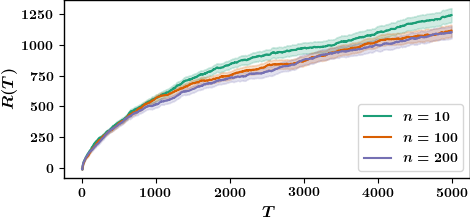
      (a) $R(T)$ vs $T$ for TSDE-MF

      

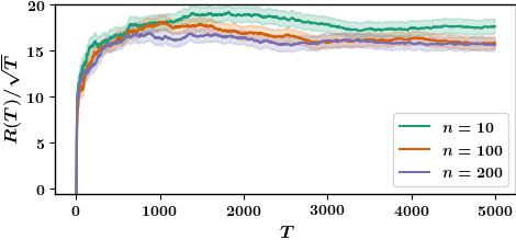
      (b) $R(T)/\sqrt{T}$ vs $T$ for TSDE-MF

      

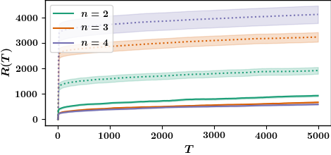
      (c) TSDE-MF (solid) vs TSDE (dashed)

      Figure 1: Expected regret vs time.

      Proof.

      We provide an outline of the proof. See the supplementary file for complete details.

      The first term $\breve{R}^{i,m}_{0}(T)$ can be bounded using the basic property of Thompson sampling: for any measurable function $f$, $\mathbb{E}[f(\breve{\theta}^{m}_{k})]=\mathbb{E}[f(\breve{\theta}^{m})]$ because $\breve{\theta}^{m}_{k}$ is a sample from the posterior distribution on $\breve{\theta}^{m}$.

      Note that the second term $\breve{R}^{i,m}_{1}(T)$ is a telescopic sum, which we can simplify to establish

      $$\breve{R}^{i,m}_{1}(T)\leq\mathcal{O}\bigl{(}\mathbb{E}[\breve{K}^{m}_{T}(\breve{X}^{i}_{T})^{2}]\bigr{)},$$

      where $\breve{X}^{i}_{t}=\max_{1\leq t\leq T}\|\breve{x}^{i}_{t}\|$ is the maximum norm of the relative state along the entire trajectory. The final bound on $\breve{R}^{i,m}_{1}(T)$ can be obtained by bounding $\breve{K}^{m}_{T}$ and $\mathbb{E}[(\breve{X}^{i}_{T})^{2}]$.

      Using the sampling condition for $\breve{p}^{m}_{t}$ and an existing bound in the literature, we first establish that

      $$\breve{R}_{2}^{i}(T)\leq\sqrt{\textstyle\mathbb{E}\big{[}(\breve{X}_{T}^{i})^{2}\sum_{t=1}^{T}(\breve{z}_{t}^{i})^{\intercal}\breve{\Sigma}^{m}_{t}\breve{z}_{t}^{i}\big{]}}\times\tilde{\mathcal{O}}(\sqrt{T})$$

      Then, we upper bound $(\breve{z}_{t}^{i})^{\intercal}\breve{\Sigma}^{m}_{t}\breve{z}_{t}^{i}$ by $(\breve{z}_{t}^{j^{m}_{t}})^{\intercal}\breve{\Sigma}^{m}_{t}\breve{z}_{t}^{j^{m}_{t}}$ which follows from the definition of $j^{m}_{t}$. Finally, we show that $\mathbb{E}[(\breve{X}_{T}^{i})^{2}\sum_{t}(\breve{z}_{t}^{j^{m}_{t}})^{\intercal}\breve{\Sigma}^{m}_{t}\breve{z}_{t}^{j^{m}_{t}}]$ is $\tilde{\mathcal{O}}(1)$ using the fact that $(\breve{\Sigma}^{m}_{t})^{-1}$ is obtained by linearly combining $\bigl{\{}\breve{z}_{s}^{j^{m}_{s}}\bigl{(}\breve{z}_{s}^{j^{m}_{s}}\bigr{)}^{\mathchoice{\raisebox{0.0pt}{$\displaystyle\intercal$}}{\raisebox{0.0pt}{$\textstyle\intercal$}}{\raisebox{0.0pt}{$\scriptstyle\intercal$}}{\raisebox{0.0pt}{$\scriptscriptstyle\intercal$}}}\bigr{\}}_{1\leq s<t}$ as in (18b).

      Combining the three bounds in Lemma 4, we get that

      $$\breve{R}^{i,m}(T)\leq\tilde{\mathcal{O}}(\breve{\sigma}^{2}d_{x}^{0.5}(d_{x}+d_{u})\sqrt{T}).$$ (25)

      By subsituting (22) and (25) in (21), we get the result of Theorem 2.

      5 Numerical Experiments

      In this section, we illustrate the performance of TSDE-MF for a homogeneous (i.e., $|M|=1$) mean-field LQ system for different values of the number $n$ of agents. See supplementary file for the choice of parameters.

      Empirical evaluation of regret:

      We run the system for $500$ different sample paths and plot the mean and standard deviation of the expected regret $R(T)$ for $T=5000$. The regret for different values of $n$ is shown in 1(a)–1(b). As seen from the plots, the regret reduces with the number of agents and $R(T)/\sqrt{T}$ converges to a constant. Thus, the empirical regret matches the upper bound of $\tilde{\mathcal{O}}((1+\frac{1}{n})\sqrt{T})$ obtained in Theorem 2.

      Comparison with naive TSDE algorithm:

      We compare the performance of TSDE-MF with that of directly using the TSDE algorithm presented in Ouyang et al. (2017, 2019) for different values of $n$. The results are shown in Fig. 1(c). As seen from the plots, the regret of TSDE-MF is smaller than TSDE but more importantly, the regret of TSDE-MF reduces with $n$ while that of TSDE increases with $n$. This matches their respective upper bounds of $\tilde{\mathcal{O}}((1+\frac{1}{n})\sqrt{T})$ and $\tilde{\mathcal{O}}(n^{1.5}\sqrt{T})$. These plots clearly illustrate the significance of our results even for small values of $n$.

      6 Conclusion

      We consider the problem of controlling an unknown LQ mean-field team. The planning solution (i.e., when the model is known) for mean-field teams is obtained by solving the mean-field system and the relative systems separately. Inspired by this feature, we propose a TS-based learning algorithm TSDE-MF which separately tracks the parameters $\bar{\theta}$ and $\breve{\theta}^{m}$ of the mean-field and the relative systems, respectively. The part of the TSDE-MF algorithm that learns the mean-field system is similar to the TSDE algorithm for single agent LQ systems proposed in Ouyang et al. (2017, 2019) and its regret can be bounded using the results of Ouyang et al. (2017, 2019). However, the part of the TSDE-MF algorithm that learns the relative component is different and we cannot directly use the results of Ouyang et al. (2017, 2019) to bound its regret. Our main technical contribution is to provide a bound on the regret on the relative system, which allows us to bound the total regret under TSDE-MF.

      Distributed implementation of the algorithm:

      It is possible to implement Algorithm 1 in a distributed manner as follows. Instead of a centralized coordinator which collects all the observations and computes all the controls, we can consider an alternative implementation in which there is an actor $\mathcal{A}^{m}$ associated with type $m$ and a mean-field actor $\bar{\mathcal{A}}$. Each agent observes its local state and action. The actor $\mathcal{A}^{m}$ for type $m$ computes $(j^{m}_{t},\bar{x}^{m}_{t})$ using a distributed algorithm, sends $\bar{x}^{m}_{t}$ to the mean-field actor, and locally computes $\breve{\mathsf{L}}^{m}(\breve{\theta}_{k})$. The mean-field actor computes $\bar{\mathsf{L}}(\bar{\theta}_{k})$ and sends the $m$-th block column $\bar{\mathsf{L}}^{m}(\bar{\theta}_{k})$ to actors $\mathcal{A}^{m}$. Each actor $\mathcal{A}^{m}$ then sends $(\bar{x}^{m}_{t},\bar{\mathsf{L}}^{m}(\bar{\theta}_{k}),\breve{\mathsf{L}}^{m}(\breve{\theta}_{k}))$ to each agent of type $m$ using a distributed algorithm. Each agent then applies the control law (11).

      Acknowledgments

      The work of AM was supported in part by the Innovation for Defence Excellence and Security (IDEaS) Program of the Canadian Department of National Defence through grant CFPMN2-30.

      Appendix A Appendix: Regret Analysis

      A.1 Preliminary Results

      The analysis does not depend on the type $m$ of the agent. So for simplicity, we will omit the superscript $m$ in all the proofs in the appendix.

      Since $\breve{S}(\cdot)$ and $\breve{L}(\cdot)$ are continuous functions on a compact set $\breve{\Theta}$, there exist finite constants $\breve{M}_{J},\breve{M}_{\breve{\theta}},\breve{M}_{S},\breve{M}_{L}$ such that $\operatorname{Tr}(\breve{S}(\breve{\theta}))\leq\breve{M}_{J},\|\breve{\theta}\|\leq\breve{M}_{\breve{\theta}},\|\breve{S}(\breve{\theta})\|\leq\breve{M}_{S}$ and $\|[I,\breve{L}(\breve{\theta})^{\mathchoice{\raisebox{0.0pt}{$\displaystyle\intercal$}}{\raisebox{0.0pt}{$\textstyle\intercal$}}{\raisebox{0.0pt}{$\scriptstyle\intercal$}}{\raisebox{0.0pt}{$\scriptscriptstyle\intercal$}}}]\|\leq\breve{M}_{L}$ for all $\breve{\theta}\in\breve{\Theta}$ where $\|\cdot\|$ is the induced matrix norm.

      Let $\breve{X}^{i}_{T}=\max_{1\leq t\leq T}\|\breve{x}^{i}_{t}\|$ be the maximum norm of the relative state along the entire trajectory. The next bound follows from Ouyang et al. (2019)[Lemma 2].

      For any $q\geq 1$ and any $T$ we have

      $$\mathbb{E}\Big{[}(\breve{X}_{T}^{i})^{q}\Big{]} \leq\breve{\sigma}^{q}\mathcal{O}\Big{(}\log(T)(1-\delta)^{-q}\Big{)}$$

      where $\delta$ is as defined in (A5).

      The following lemma gives an almost sure upper bound on the number of episodes $\breve{K}_{T}$.

      The number of episodes $\breve{K}_{T}$ is bounded as follows:

      $$\breve{K}_{T} \leq\mathcal{O}\left(\sqrt{(d_{x}+d_{u})T\log\left(\frac{1}{\breve{\sigma}^{2}}\sum_{t}(\breve{X}_{T}^{j_{t}})^{2}\right)}\right)$$

      Proof.

      We can follow the same sketch as in proof of Lemma 3 in Ouyang et al. (2019). Let $\breve{\eta}-1$ be the number of times the second stopping criterion is triggered for $\breve{p}_{t}$. Using the analysis in the proof of Lemma 3 in Ouyang et al. (2019), we can get the following

      $$\breve{K}_{T}\leq\sqrt{2\breve{\eta}T}.$$ (26)

      Since the second stopping criterion is triggered whenever the determinant of sample covariance is halved, we have

      $$\det(\breve{\Sigma}^{-1}_{T})\geq 2^{\breve{\eta}-1}\det(\breve{\Sigma}^{-1}_{1})$$

      Let $d=d_{x}+d_{u}$. Since $(\frac{1}{d}\operatorname{Tr}(\breve{\Sigma}_{T}^{-1}))^{d}\geq\det(\breve{\Sigma}_{T}^{-1})$, we have

      $$\operatorname{Tr}(\breve{\Sigma}_{T}^{-1}) \geq d(\det(\breve{\Sigma}_{T}^{-1}))^{1/d}\geq d\times 2^{(\breve{\eta}-1)/d}(\det(\breve{\Sigma}^{-1}_{1}))^{1/d}$$

      $$\geq d\times 2^{(\breve{\eta}-1)/d}\breve{\lambda}_{min}$$

      where $\breve{\lambda}_{min}$ is the minimum eigenvalue of $\breve{\Sigma}^{-1}_{1}$.

      Using (18b) we have,

      $$\breve{\Sigma}_{T}^{-1}=\breve{\Sigma}_{1}^{-1}+\sum_{t=1}^{T-1}\frac{1}{\breve{\sigma}^{2}}\breve{z}_{t}^{j_{t}}(\breve{z}_{t}^{j_{t}})^{\intercal}.$$

      Therefore $\operatorname{Tr}(\breve{\Sigma}_{T}^{-1})=\operatorname{Tr}(\breve{\Sigma}_{1}^{-1})+\sum_{t=1}^{T-1}\frac{1}{\breve{\sigma}^{2}}\operatorname{Tr}(\breve{z}_{t}^{j_{t}}(\breve{z}_{t}^{j_{t}})^{\intercal})$. Note that $\operatorname{Tr}(\breve{z}_{t}^{j_{t}}(\breve{z}_{t}^{j_{t}})^{\intercal})=\operatorname{Tr}((\breve{z}_{t}^{j_{t}})^{\intercal}\breve{z}_{t}^{j_{t}})=\|\breve{z}_{t}^{j_{t}}\|^{2}$. Thus,

      $$d\times 2^{(\breve{\eta}-1)/d}\breve{\lambda}_{min} \leq\operatorname{Tr}(\breve{\Sigma}_{1}^{-1})+\sum_{t=1}^{T-1}\frac{1}{\breve{\sigma}^{2}}||\breve{z}_{t}^{j_{t}}||^{2}$$

      Then,

      $$\breve{\eta}\leq 1+\frac{d}{\log 2}\log\left(\frac{1}{d\breve{\lambda}_{min}}\left(\operatorname{Tr}(\breve{\Sigma}_{1}^{-1}+\sum_{t=1}^{T-1}\frac{1}{\breve{\sigma}^{2}}||\breve{z}_{t}^{j_{t}}||^{2}\right)\right)$$

      $$=\mathcal{O}\left(d\log\left(\frac{1}{\breve{\sigma}^{2}}\sum_{t=1}^{T-1}||\breve{z}_{t}^{j_{t}}||^{2}\right)\right).$$

      Note that, $||\breve{z}_{t}^{j_{t}}||=||[I,L(\breve{\theta})^{\intercal}]^{\intercal}\breve{x}_{t}^{j_{t}}||\leq\breve{M}_{L}||\breve{x}_{t}^{j_{t}}||\leq\breve{M}_{L}\breve{X}_{T}^{j_{t}}$. Consequently,

      $$\breve{\eta}\leq \mathcal{O}\Big{(}d\log\Big{(}\frac{1}{\breve{\sigma}^{2}}\sum_{t=1}^{T-1}(\breve{X}_{T}^{j_{t}})^{2}\Big{)}\Big{)}$$

      Therefore, combining the above inequality with (26) we get,

      $$\breve{K}_{T}\leq\mathcal{O}\left(\sqrt{(d_{x}+d_{u})T\log\Big{(}\frac{1}{\breve{\sigma}^{2}}\sum_{t=1}^{T-1}(\breve{X}_{T}^{j_{t}})^{2}\Big{)}}\right)$$ (27)

      A.2 Proof of Lemma 4

      Proof.

      We will bound each part separately.

      1) Bounding $\breve{R}^{i}_{0}(T)$: From monotone convergence theorem, we have

      $$\breve{R}^{i}_{0}(T)= \mathbb{E}\Big{[}\sum_{k=1}^{\infty}\mathds{1}_{\{\breve{t}_{k}\leq T\}}\breve{T}_{k}\breve{J}(\breve{\theta}_{k})\Big{]}-T\mathbb{E}\Big{[}\breve{J}(\breve{\theta})\Big{]}$$

      $$= \sum_{k=1}^{\infty}\mathbb{E}\Big{[}\mathds{1}_{\{\breve{t}_{k}\leq T\}}\breve{T}_{k}\breve{J}(\breve{\theta}_{k})\Big{]}-T\mathbb{E}\Big{[}\breve{J}(\breve{\theta})\Big{]}.$$

      Note that the first stopping criterion of TSDE-MF ensures that $\breve{T}_{k}\leq\breve{T}_{k-1}+1$ for all $k$. Since $\breve{J}(\breve{\theta}_{k})\geq 0$, each term in the first summation satisfies,

      $$\mathbb{E}\Big{[}\mathds{1}_{\{\breve{t}_{k}\leq T\}}\breve{T}_{k}\breve{J}(\breve{\theta}_{k})\Big{]}\leq \mathbb{E}\Big{[}\mathds{1}_{\{\breve{t}_{k}\leq T\}}(\breve{T}_{k-1}+1)\breve{J}(\breve{\theta}_{k})\Big{]}.$$

      Note that $\mathds{1}_{\{\breve{t}_{k}\leq T\}}(\breve{T}_{k-1}+1)$ is measurable with respect to $\sigma(\{\breve{x}_{s}^{j_{s}},\breve{u}_{s}^{j_{s}},\breve{x}_{s+1}^{j_{s}}\}_{1\leq s<\breve{t}_{k}})$. Then, Lemma 4 of Ouyang et al. (2019) gives

      $$\mathbb{E}\Big{[}\mathds{1}_{\{\breve{t}_{k}\leq T\}}(\breve{T}_{k-1}+1)\breve{J}(\breve{\theta}_{k})\Big{]}=\mathbb{E}\Big{[}\mathds{1}_{\{\breve{t}_{k}\leq T\}}(\breve{T}_{k-1}+1)\breve{J}(\breve{\theta})\Big{]}.$$

      Combining the above equations, we get

      $$\breve{R}^{i}_{0}(T)\leq \sum_{k=1}^{\infty}\mathbb{E}\Big{[}\mathds{1}_{\{\breve{t}_{k}\leq T\}}(\breve{T}_{k-1}+1)\breve{J}(\breve{\theta})\Big{]}-T\mathbb{E}\Big{[}\breve{J}(\breve{\theta})\Big{]}$$

      $$= \mathbb{E}\Big{[}\sum_{k=1}^{\breve{K}_{T}}(\breve{T}_{k-1}+1)\breve{J}(\breve{\theta})\Big{]}-T\mathbb{E}\Big{[}\breve{J}(\breve{\theta})\Big{]}$$

      $$= \mathbb{E}\Big{[}\breve{K}_{T}\breve{J}(\breve{\theta})\Big{]}+\mathbb{E}\Big{[}\Big{(}\sum_{k=1}^{\breve{K}_{T}}\breve{T}_{k-1}-T\Big{)}\breve{J}(\breve{\theta})\Big{]}$$

      $$\leq \breve{M}_{J}\breve{\sigma}^{2}\mathbb{E}\Big{[}\breve{K}_{T}\Big{]}$$

      where the last equality holds because $\breve{J}(\breve{\theta})=\breve{\sigma}^{2}\operatorname{Tr}(\breve{S}(\breve{\theta}))\leq\breve{\sigma}^{2}\breve{M}_{J}$ and $\sum_{k=1}^{\breve{K}_{T}}\breve{T}_{k-1}\leq T$.

      2) Bounding $\breve{R}^{i}_{1}(T)$:

      $$\breve{R}^{i}_{1}(T)= \mathbb{E}\Big{[}\sum_{k=1}^{\breve{K}_{T}}\sum_{t=\breve{t}_{k}}^{\breve{t}_{k+1}-1}\Big{[}(\breve{x}_{t}^{i})^{\intercal}\breve{S}(\breve{\theta}_{k})\breve{x}_{t}^{i}-(\breve{x}_{t+1}^{i})^{\intercal}\breve{S}(\breve{\theta}_{k})\breve{x}_{t+1}^{i}\Big{]}\Big{]}$$

      $$= \mathbb{E}\Big{[}\sum_{k=1}^{\breve{K}_{T}}\Big{[}(\breve{x}^{i}_{\breve{t}_{k}})^{\intercal}\breve{S}(\breve{\theta}_{k})\breve{x}_{\breve{t}_{k}}^{i}-(\breve{x}_{\breve{t}_{k+1}}^{i})^{\intercal}\breve{S}(\breve{\theta}_{k})\breve{x}_{\breve{t}_{k+1}}^{i}\Big{]}\Big{]}$$

      $$\leq \mathbb{E}\Big{[}\sum_{k=1}^{\breve{K}_{T}}(\breve{x}^{i}_{\breve{t}_{k}})^{\intercal}\breve{S}(\breve{\theta}_{k})\breve{x}_{\breve{t}_{k}}^{i}\Big{]}.$$

      Since $||\breve{S}(\breve{\theta}_{k})||\leq\breve{M}_{S}$, we obtain

      $$\breve{R}^{i}_{1}(T)\leq \mathbb{E}\Big{[}\sum_{k=1}^{\breve{K}_{T}}\breve{M}_{S}\|\breve{x}_{\breve{t}_{k}}^{i}\|^{2}\Big{]}\leq\breve{M}_{S}\mathbb{E}\Big{[}\breve{K}_{T}(\breve{X}_{T}^{i})^{2}\Big{]}.$$

      Now, from Lemma A.1, $\breve{K}_{T}\leq\mathcal{O}(\sqrt{T\log(\frac{\sum_{t=1}^{T}(\breve{X}_{T}^{j_{t}})^{2}}{\breve{\sigma}^{2}}))}$. Thus, we have $\breve{R}^{i}_{1}(T)\leq\mathcal{O}\left(\sqrt{T}\mathbb{E}\Big{[}(\breve{X}_{T}^{i})^{2}\sqrt{\log\left(\frac{\sum_{t=1}^{T}(\breve{X}_{T}^{j_{t}})^{2}}{\breve{\sigma}^{2}}\right)}\Big{]}\right)$. Then, using Cauchy-Schwarz we have,

      $$\mathbb{E}\left[(\breve{X}_{T}^{i})^{2}\sqrt{\log\left(\frac{\sum_{t=1}^{T}(\breve{X}_{T}^{j_{t}})^{2}}{\breve{\sigma}^{2}}\right)}\right] \leq\sqrt{\mathbb{E}\Big{[}(\breve{X}_{T}^{i})^{4}\Big{]}~{}~{}\mathbb{E}\Big{[}\log\left(\frac{\sum_{t=1}^{T}(\breve{X}_{T}^{j_{t}})^{2}}{\breve{\sigma}^{2}}\right)\Big{]}}$$

      $$\leq\sqrt{\mathbb{E}\Big{[}(\breve{X}_{T}^{i})^{4}\Big{]}\log\left(\sum_{t=1}^{T}\frac{\mathbb{E}(\breve{X}_{T}^{j_{t}})^{2}}{\breve{\sigma}^{2}}\right)}\leq\tilde{\mathcal{O}}(\breve{\sigma}^{2})$$

      where the last inequality follows from Lemma A.1. Therefore, we have $\breve{R}^{i}_{1}(T)\leq\tilde{\mathcal{O}}\left(\breve{\sigma}^{2}~{}\sqrt{T}\right)$.

      3) Bounding $\breve{R}^{i}_{2}(T)$: Each term inside the expectation of $\breve{R}^{i}_{2}$ is equal to

      $$\|\breve{S}^{0.5}(\breve{\theta}_{k})\breve{\theta}^{\intercal}\breve{z}_{t}^{i}\|^{2}-\|\breve{S}^{0.5}(\breve{\theta}_{k})\breve{\theta}_{k}^{\intercal}\breve{z}_{t}^{i}\|^{2}\leq \left(\|\breve{S}^{0.5}(\breve{\theta}_{k})\breve{\theta}^{\intercal}\breve{z}_{t}^{i}\|+\|\breve{S}^{0.5}(\breve{\theta}_{k})\breve{\theta}_{k}^{\intercal}\breve{z}_{t}^{i}\|\right)||\breve{S}^{0.5}(\breve{\theta}_{k})(\breve{\theta}-\breve{\theta}_{k})^{\intercal}\breve{z}_{t}^{i}||$$

      $$\leq 2\breve{M}_{S}\breve{M}_{\theta}\breve{M}_{L}\breve{X}_{T}^{i}||(\breve{\theta}-\breve{\theta}_{k})^{\intercal}\breve{z}_{t}^{i}||$$

      since $\|\breve{S}^{0.5}(\breve{\theta}_{k})\breve{\phi}^{\intercal}\breve{z}_{t}^{i}\|\leq\breve{M}_{S}^{0.5}\breve{M}_{\theta}\breve{M}_{L}\breve{X}_{T}^{i}$ for $\breve{\phi}=\breve{\theta}$ or $\breve{\phi}=\breve{\theta}_{k}$. Therefore,

      $$\breve{R}^{i}_{2}(T)\leq 2\breve{M}_{S}\breve{M}_{\theta}\breve{M}_{L}\mathbb{E}\Big{[}\breve{X}_{T}^{i}\sum_{k=1}^{\breve{K}_{T}}\sum_{t=\breve{t}_{k}}^{\breve{t}_{k+1}-1}\|(\breve{\theta}-\breve{\theta}_{k})^{\intercal}\breve{z}_{t}^{i}\|\Big{]}.$$ (28)

      From Cauchy-Schwarz inequality, we have

      $$\mathbb{E}\Big{[}\breve{X}_{T}^{i}\sum_{k=1}^{\breve{K}_{T}}\sum_{t=\breve{t}_{k}}^{\breve{t}_{k+1}-1}\|(\breve{\theta}-\breve{\theta}_{k})^{\intercal}\breve{z}_{t}^{i}\|\Big{]} =\mathbb{E}\Big{[}\breve{X}_{T}^{i}\sum_{k=1}^{\breve{K}_{T}}\sum_{t=\breve{t}_{k}}^{\breve{t}_{k+1}-1}\|(\breve{\Sigma}^{-0.5}_{t}(\breve{\theta}-\breve{\theta}_{k}))^{\intercal}\breve{\Sigma}^{0.5}_{t}\breve{z}_{t}^{i}\|\Big{]}$$

      $$\leq\mathbb{E}\Big{[}\sum_{k=1}^{\breve{K}_{T}}\sum_{t=\breve{t}_{k}}^{\breve{t}_{k+1}-1}\|\breve{\Sigma}^{-0.5}_{t}(\breve{\theta}-\breve{\theta}_{k})\|\times\breve{X}_{T}^{i}\|\breve{\Sigma}^{0.5}_{t}\breve{z}_{t}^{i}\|\Big{]}$$

      $$\leq\sqrt{\mathbb{E}\Big{[}\sum_{k=1}^{\breve{K}_{T}}\sum_{t=\breve{t}_{k}}^{\breve{t}_{k+1}-1}\|\breve{\Sigma}^{-0.5}_{t}(\breve{\theta}-\breve{\theta}_{k})\|^{2}\Big{]}}\sqrt{\mathbb{E}\Big{[}\sum_{k=1}^{\breve{K}_{T}}\sum_{t=\breve{t}_{k}}^{\breve{t}_{k+1}-1}(\breve{X}_{T}^{i})^{2}\|\breve{\Sigma}^{0.5}_{t}\breve{z}_{t}^{i}\|^{2}\Big{]}}$$ (29)

      From Lemma 10 in Ouyang et al. (2019), the first part of (29) is bounded by

      $$\mathbb{E}\Big{[}\sum_{k=1}^{\breve{K}_{T}}\sum_{t=\breve{t}_{k}}^{\breve{t}_{k+1}-1}\|\breve{\Sigma}^{-0.5}_{t}(\breve{\theta}-\breve{\theta}_{k})\|^{2}\Big{]}\leq 4d_{x}d(T+\mathbb{E}[\breve{K}_{T}]).$$ (30)

      For the second part of the bound in (29), we note that

      $$\sum_{t}||\breve{\Sigma}^{0.5}_{t}\breve{z}_{t}^{i}||^{2} =\sum_{t=1}^{T}(\breve{z}_{t}^{i})^{\intercal}\breve{\Sigma}_{t}\breve{z}_{t}^{i}$$

      $$\leq\sum_{t=1}^{T}\max\left(1,\frac{\breve{M}_{L}^{2}(\breve{X}_{T}^{i})^{2}}{\breve{\lambda}_{min}}\right)\min(1,(\breve{z}_{t}^{i})^{\intercal}\breve{\Sigma}_{t}\breve{z}_{t}^{i})$$

      $$\leq\sum_{t=1}^{T}\left(1+\frac{\breve{M}_{L}^{2}(\breve{X}_{T}^{i})^{2}}{\breve{\lambda}_{min}}\right)\min(1,(\breve{z}_{t}^{j_{t}})^{\intercal}\breve{\Sigma}_{t}\breve{z}_{t}^{j_{t}})$$ (31)

      where the last inequality follows from the definition of $j_{t}$. Using Lemma 8 of Abbasi-Yadkori and Szepesvári (2015) we have

      $$\sum_{t=1}^{T}\min(1,(\breve{z}_{t}^{j_{t}})^{\intercal}\breve{\Sigma}_{t}\breve{z}_{t}^{j_{t}})\leq 2d\log\left(\frac{\operatorname{Tr}(\breve{\Sigma}_{1}^{-1})+\breve{M}_{L}^{2}\sum_{t=1}^{T}(X_{T}^{j_{t}})^{2}}{d}\right)$$ (32)

      Combining (31) and (32), we can bound the second part of (29) to the following

      $$\mathbb{E}\Big{[}\sum_{t}(\breve{X}_{T}^{i})^{2}||\breve{\Sigma}^{0.5}_{t}\breve{z}_{t}^{i}||^{2}\Big{]}\leq\mathcal{O}\Big{(}\mathbb{E}\Big{[}(\breve{X}_{T}^{i})^{4}\log(\sum_{t=1}^{T}(\breve{X}_{T}^{j_{t}})^{2})\Big{]}+\mathbb{E}\Big{[}(\breve{X}_{T}^{i})^{2}\log(\sum_{t=1}^{T}(\breve{X}_{T}^{j_{t}})^{2})\Big{]}\Big{)}.$$ (33)

      The bound on $\breve{R}^{i}_{2}(T)$ in Lemma 4 then follows by combining (28)-(33) with the bound on $\mathbb{E}\Big{[}(\breve{X}_{T}^{i})^{q}\log(\sum_{t=1}^{T}(\breve{X}_{T}^{j_{t}})^{2})\Big{]}$ for $q=2,4$ in Lemma A.2 in the appendix.

      For any $q\geq 1$, we have

      $$\mathbb{E}\left[(\breve{X}_{T}^{i})^{q}\log(\sum_{t}(\breve{X}_{T}^{j_{t}})^{2})\right] \leq\left(\breve{\sigma}\right)^{q}\tilde{\mathcal{O}}(1)$$ (34)

      Proof.

      $$\mathbb{E}\left[(\breve{X}_{T}^{i})^{q}\log(\sum_{t}(\breve{X}_{T}^{j_{t}})^{2})\right] \leq\mathbb{E}\left[(\breve{X}_{T}^{i})^{q}\log(\max(e,\sum_{t}(\breve{X}_{T}^{j_{t}})^{2}))\right]$$

      $$\leq\sqrt{\mathbb{E}[(\breve{X}_{T}^{i})^{2q}]~{}~{}\mathbb{E}[\log^{2}\big{(}\max(e,\sum_{t}\breve{X}_{T}^{j_{t}})^{2})\big{)}]}$$

      where the second inequality follows from the Cauchy-Schwarz inequality. Now, $\log^{2}(x)$ is a concave function for $x\geq e$. Therefore, using Jensen’s inequality we can write,

      $$\mathbb{E}\log^{2}\big{(}\max(e,\sum_{t}\breve{X}_{T}^{j_{t}})^{2})\big{)} \leq\log^{2}(\mathbb{E}\max(e,\sum_{t}\breve{X}_{T}^{j_{t}})^{2}))$$

      $$\leq\log^{2}\left(e+\mathbb{E}(\sum_{t}\breve{X}_{T}^{j_{t}})^{2})\right)$$

      $$\leq\log^{2}\left(e+T\mathcal{O}(\breve{\sigma}^{2}~{}\log T)\right)$$

      $$=\tilde{\mathcal{O}}(1)$$

      where we used Lemma 4 in the last inequality. Similarly, $\mathbb{E}[(\breve{X}_{T}^{i})^{2q}]\leq\left(\breve{\sigma}\right)^{2q}\mathcal{O}(\log T)$. Therefore, combining the above inequalities we have the following:

      $$\mathbb{E}\left[(\breve{X}_{T}^{i})^{q}\log(\sum_{t}(\breve{X}_{T}^{j_{t}})^{2})\right] \leq\sqrt{\mathbb{E}[(\breve{X}_{T}^{i})^{2q}]~{}~{}\mathbb{E}\Big{[}\log^{2}\left(\max(e,\sum_{t}\breve{X}_{T}^{j_{t}})^{2})\right)\Big{]}}$$

      $$\leq\breve{\sigma}^{q}\tilde{\mathcal{O}}(1)$$

      Appendix B Simulation Details

      We consider homogeneous scalar system ($\lvert K\rvert=1$) with $\mathsf{A}=1,\mathsf{B}=0.3,\mathsf{D}=0.5,\mathsf{E}=0.2,\mathsf{Q}=1,\bar{\mathsf{Q}}=1,\mathsf{R}=1$,and $\bar{\mathsf{R}}=0.5$. We set the local noise variance $\sigma_{w}^{2}=1$.

      For the regret plots in Figure 1(a),1(b), we set the common noise variance to $\sigma_{v}^{2}+\sigma_{v^{0}}^{2}=1$. The prior distribution used in the simulation are set according to (A3) and (A4) with $\breve{\mu}(\ell)=[1,1]$, $\bar{\mu}(\ell)=[1,1]$, $\bar{\Sigma}_{1}=I$, and $\breve{\Sigma}_{1}=I$, $\breve{\Theta}=\{\breve{\theta}:\mathsf{A}+\mathsf{B}\breve{\mathsf{L}}(\breve{\theta})\leq\delta\}$, $\bar{\Theta}=\{\bar{\theta}:\mathsf{A}+\mathsf{D}+(\mathsf{B}+\mathsf{E})\bar{\mathsf{L}}(\bar{\theta})\leq\delta\}$ and $\delta=0.99$.

      In the comparison of TSDE-MF method with TSDE in Figure 1(c), we consider the same dynamics and cost parameters as above but without common noise (i.e. $\sigma_{v}^{2}+\sigma_{v^{0}}^{2}=0$). We set the prior distribution parameters to $\breve{\mu}(\ell)=[0,0]$, $\bar{\mu}(\ell)=[0,0]$, $\bar{\Sigma}_{1}=I$, and $\breve{\Sigma}_{1}=I$ and $\delta=2.3$ in the definition of $\bar{\Theta},\breve{\Theta}$. Note that even though $\delta=2.3$ does not satisfy (A5), the results show that TSDE-MF continues to have good performance in practice.

      Appendix C Comparison with other agent selection schemes

      In TSDE-MF, we update the posterior probability $\breve{p}_{t}$ on $\breve{\theta}$ using $\{x^{i^{*}_{s}}_{s},u^{i^{*}_{s}}_{s},x^{i^{*}_{s}}_{s+1}\}_{1\leq s<t}$, where $i^{*}_{s}=\arg\max_{i\in N}(\breve{z}^{i}_{s})^{\mathchoice{\raisebox{0.0pt}{$\displaystyle\intercal$}}{\raisebox{0.0pt}{$\textstyle\intercal$}}{\raisebox{0.0pt}{$\scriptstyle\intercal$}}{\raisebox{0.0pt}{$\scriptscriptstyle\intercal$}}}\breve{\Sigma}_{s}\breve{z}^{i}_{s}$. This particular choice of the agent selection rule implies that while deriving a bound on $\breve{R}^{i}_{2}(T)$, we can upper bound $\sum_{t=1}^{T}(\breve{z}^{i}_{t})^{\mathchoice{\raisebox{0.0pt}{$\displaystyle\intercal$}}{\raisebox{0.0pt}{$\textstyle\intercal$}}{\raisebox{0.0pt}{$\scriptstyle\intercal$}}{\raisebox{0.0pt}{$\scriptscriptstyle\intercal$}}}\breve{\Sigma}_{t}\breve{z}^{i}_{t}$ by $\sum_{t=1}^{T}(\breve{z}^{i^{*}_{t}}_{t})^{\mathchoice{\raisebox{0.0pt}{$\displaystyle\intercal$}}{\raisebox{0.0pt}{$\textstyle\intercal$}}{\raisebox{0.0pt}{$\scriptstyle\intercal$}}{\raisebox{0.0pt}{$\scriptscriptstyle\intercal$}}}\breve{\Sigma}_{t}\breve{z}^{i^{*}_{t}}_{t}$. This, in turn, allows us to bound the regret of $\breve{R}^{i}_{2}(T)$ in terms of $\mathbb{E}[\log^{2}(\sum_{t=1}^{T}(X^{i^{*}_{t}}_{T})^{2})]$, which we show is $\tilde{O}(1)$.

      There are three other choices for the agent selection rule: (i) picking a specific agent, or (ii) picking an agent at random, or (iii) using the entire trajectory $(\bm{\breve{x}}_{1:t},\bm{\breve{u}}_{1:t-1})$, where $\bm{\breve{x}}_{t}=(\breve{x}^{i}_{t})_{i\in N}$ and $\bm{\breve{u}}_{t}=(\breve{u}^{i}_{t})_{i\in N}$.

      

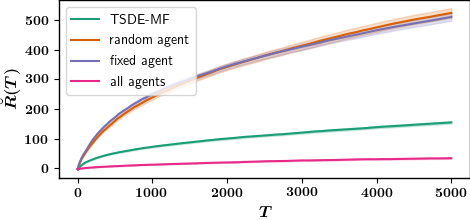
      (a) $\breve{R}(T)$ vs $T$

      

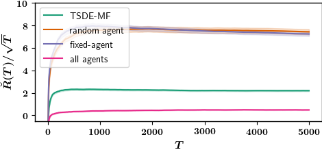
      (b) $\breve{R}(T)/\sqrt{T}$ vs $T$

      Figure 2: Impact of different agent selection schemes on expected regret.

      If we follow approach (i) and arbitrarily pick an agent, say $j$, and update the posterior distribution $\breve{p}_{t}$ on $\breve{\theta}$ using $(x^{j}_{1:t},u^{j}_{1:t-1})$. This would mean that we can directly use the result of Ouyang et al. (2017, 2019) to bound the regret of $\breve{R}^{j}(T)$. However, we would still need to bound $\breve{R}^{i}(T)$ for $i\neq j$. In this case, we can follow the argument similar to one presented in the supplementary file to bound $\breve{R}^{i}_{0}(T)$ and $\breve{R}^{i}_{1}(T)$, but the bound on $\breve{R}^{i}_{2}(T)$ does not work because we are not able to bound $\sum_{t=1}^{T}(\breve{z}^{i}_{t})^{\mathchoice{\raisebox{0.0pt}{$\displaystyle\intercal$}}{\raisebox{0.0pt}{$\textstyle\intercal$}}{\raisebox{0.0pt}{$\scriptstyle\intercal$}}{\raisebox{0.0pt}{$\scriptscriptstyle\intercal$}}}\breve{\Sigma}_{t}\breve{z}^{i}_{t}$ in terms of an expression involving $X^{j}_{T}$. Similar limitations hold for alternative (ii).

      We conducted numerical experiments to check if these alternatives perform better in practice, which are presented in Fig. 2, where we show $\breve{R}(T)=\frac{1}{n}\sum_{i=1}^{n}\breve{R}^{i}(T)$ for the system model analyzed in Sec. 5. For alternatives (i) and (ii), their regret orders appear to be bounded by $\tilde{\mathcal{O}}(\sqrt{T})$, but they clearly perform worse than the proposed method. For alternative (iii), the regret is slightly better than the proposed method. However, implementing alternative (iii) requires complete trajectory sharing among all agents. The extra computation and communication cost of alternative (iii) could hinder its application to systems with a large number of agents.

References

• Auer et al. (2002) P. Auer, N. Cesa-Bianchi, and P. Fischer. Finite-time analysis of the multiarmed bandit problem. Machine learning, 47(2-3):235–256, 2002.
• Campi and Kumar (1998) M. C. Campi and P. Kumar. Adaptive linear quadratic gaussian control: the cost-biased approach revisited. SIAM Journal on Control and Optimization, 36(6):1890–1907, 1998.
• Abbasi-Yadkori and Szepesvári (2011) Y. Abbasi-Yadkori and C. Szepesvári. Regret bounds for the adaptive control of linear quadratic systems. In Proceedings of the 24th Annual Conference on Learning Theory, pages 1–26, 2011.
• Faradonbeh et al. (2017) M. K. S. Faradonbeh, A. Tewari, and G. Michailidis. Finite time analysis of optimal adaptive policies for linear-quadratic systems. arXiv preprint arXiv:1711.07230, 2017.
• Cohen et al. (2019) A. Cohen, T. Koren, and Y. Mansour. Learning linear-quadratic regulators efficiently with only $\sqrt{T}$ regret. arXiv preprint arXiv:1902.06223, 2019.
• Abeille and Lazaric (2020) M. Abeille and A. Lazaric. Efficient optimistic exploration in linear-quadratic regulators via lagrangian relaxation. arXiv preprint arXiv:2007.06482, 2020.
• Astrom and Wittenmark (1994) K. J. Astrom and B. Wittenmark. Adaptive Control. Addison-Wesley Longman Publishing Co., Inc., 1994.
• Dean et al. (2018) S. Dean, H. Mania, N. Matni, B. Recht, and S. Tu. Regret bounds for robust adaptive control of the linear quadratic regulator. In Advances in Neural Information Processing Systems, pages 4192–4201, 2018.
• Mania et al. (2019) H. Mania, S. Tu, and B. Recht. Certainty equivalent control of LQR is efficient. preprint arXiv:1902.07826, 2019.
• Faradonbeh et al. (2020) M. K. S. Faradonbeh, A. Tewari, and G. Michailidis. Input perturbations for adaptive control and learning. Automatica, 117:108950, 2020.
• Simchowitz and Foster (2020) M. Simchowitz and D. J. Foster. Naive exploration is optimal for online lqr. arXiv preprint arXiv:2001.09576, 2020.
• Agrawal and Goyal (2012) S. Agrawal and N. Goyal. Analysis of thompson sampling for the multi-armed bandit problem. In Conference on Learning Theory, 2012.
• Ouyang et al. (2017) Y. Ouyang, M. Gagrani, and R. Jain. Control of unknown linear systems with thompson sampling. In 55th Annual Allerton Conference on Communication, Control, and Computing, pages 1198–1205, 2017.
• Ouyang et al. (2019) Y. Ouyang, M. Gagrani, and R. Jain. Posterior sampling-based reinforcement learning for control of unknown linear systems. IEEE Transactions on Automatic Control, 2019.
• Abeille and Lazaric (2018) M. Abeille and A. Lazaric. Improved regret bounds for thompson sampling in linear quadratic control problems. In International Conference on Machine Learning, pages 1–9, 2018.
• Cassel et al. (2020) A. Cassel, A. Cohen, and T. Koren. Logarithmic regret for learning linear quadratic regulators efficiently. arXiv preprint arXiv:2002.08095, 2020.
• Lunze (1986) J. Lunze. Dynamics of strongly coupled symmetric composite systems. International Journal of Control, 44(6):1617–1640, 1986.
• Sundareshan and Elbanna (1991) M. K. Sundareshan and R. M. Elbanna. Qualitative analysis and decentralized controller synthesis for a class of large-scale systems with symmetrically interconnected subsystems. Automatica, 27(2):383–388, 1991.
• Yang and Zhang (1995) G.-H. Yang and S.-Y. Zhang. Structural properties of large-scale systems possessing similar structures. Automatica, 31(7):1011–1017, 1995.
• Hamilton and Broucke (2012) S. C. Hamilton and M. E. Broucke. Patterned linear systems. Automatica, 48(2):263–272, 2012.
• Arabneydi and Mahajan (2015) J. Arabneydi and A. Mahajan. Team-optimal solution of finite number of mean-field coupled lqg subsystems. In Proc. 54rd IEEE Conf. Decision and Control, Kyoto, Japan, Dec. 2015.
• Arabneydi and Mahajan (2016) J. Arabneydi and A. Mahajan. Linear Quadratic Mean Field Teams: Optimal and Approximately Optimal Decentralized Solutions, 2016. arXiv:1609.00056.
• Lasry and Lions (2007) J.-M. Lasry and P.-L. Lions. Mean field games. Japanese Journal of Mathematics, 2(1):229–260, 2007.
• Huang et al. (2007) M. Huang, P. E. Caines, and R. P. Malhamé. Large-population cost-coupled LQG problems with nonuniform agents: individual-mass behavior and decentralized epsilon-Nash equilibria. IEEE Transactions on Automatic Control, 52(9):1560–1571, 2007.
• Huang et al. (2012) M. Huang, P. E. Caines, and R. P. Malhamé. Social optima in mean field LQG control: centralized and decentralized strategies. IEEE Transactions on Automatic Control, 57(7):1736–1751, 2012.
• Weintraub et al. (2005) G. Y. Weintraub, C. L. Benkard, and B. V. Roy. Oblivious Equilibrium: A Mean Field Approximation for Large-Scale Dynamic Games. In Advances in Neural Information Processing Systems, pages 1489–1496, Dec. 2005.
• Weintraub et al. (2008) G. Y. Weintraub, C. L. Benkard, and B. Van Roy. Markov perfect industry dynamics with many firms. Econometrica, 76(6):1375–1411, 2008.
• Gomes et al. (2014) D. A. Gomes et al. Mean field games models—a brief survey. Dynamic Games and Applications, 4(2):110–154, 2014.
• Yang et al. (2018) Y. Yang, R. Luo, M. Li, M. Zhou, W. Zhang, and J. Wang. Mean field multi-agent reinforcement learning. In J. Dy and A. Krause, editors, Proceedings of the 35th International Conference on Machine Learning, volume 80 of Proceedings of Machine Learning Research, pages 5567–5576, Stockholmsmässan, Stockholm Sweden, 10–15 Jul 2018. PMLR.
• Subramanian and Mahajan (2019) J. Subramanian and A. Mahajan. Reinforcement learning in stationary mean-field games. In Proceedings of the 18th International Conference on Autonomous Agents and MultiAgent Systems, pages 251–259, 2019.
• Tiwari et al. (2019) N. Tiwari, A. Ghosh, and V. Aggarwal. Reinforcement learning for mean field game. arXiv preprint arXiv:1905.13357, 2019.
• Guo et al. (2019) X. Guo, A. Hu, R. Xu, and J. Zhang. Learning mean-field games. In Advances in Neural Information Processing Systems, pages 4966–4976, 2019.
• Subramanian et al. (2020) S. G. Subramanian, P. Poupart, M. E. Taylor, and N. Hegde. Multi type mean field reinforcement learning. arXiv preprint arXiv:2002.02513, 2020.
• Zhang et al. (2020) K. Zhang, E. Miehling, et al. Reinforcement learning in non-stationary discrete-time linear-quadratic mean-field games. arXiv preprint arXiv:2009.04350, 2020.
• Sternby (1977) J. Sternby. On consistency for the method of least squares using martingale theory. IEEE T. on Automatic Control, 22(3):346–352, 1977.
• Abbasi-Yadkori and Szepesvári (2015) Y. Abbasi-Yadkori and C. Szepesvári. Bayesian optimal control of smoothly parameterized systems. In UAI, 2015.