Seeing-limited imaging sky surveys – small vs. large telescopes

Abstract

Typically large telescope construction and operation costs scale up faster than their collecting area. This slows scientific progress, making it expensive and complicated to increase telescope size. We review the argument that a metric that represents the capability of an imaging survey telescopes, and that captures a wide range of science objectives, is the telescope grasp - the amount of volume of space in which a standard candle is detectable per unit time. We show that in a homogeneous Euclidean universe, and in the background-noise dominated limit, the grasp is: $\mathcal{G}\propto\Omega A_{\rm eff}^{3/4}\sigma^{-3/2}t_{\rm E}^{3/4}/(t_{\rm E}+t_{D})$, where $\Omega$ is the telescope field of view, $A_{\rm eff}$ is the effective collecting area of the telescope, $\sigma$ is the instrumental or atmospheric seeing or the pixel-size, whichever dominates, $t_{\rm E}$ is the exposure time, and $t_{\rm D}$ is the dead time. In this case, the optimal exposure time is three times the dead time. We also introduce a related metric we call the information-content grasp, which summarizes the variance of all sources observed by the telescope per unit time. We show that, in the background-noise dominated regime, the information-content grasp scales like the grasp. For seeing-dominated sky surveys, in terms of grasp, étendue, or collecting-area optimization, recent technological advancements make it more cost effective to construct multiple small telescopes rather than a single large telescope with a similar grasp or étendue. Among these key advancements are the availability of large-format back-side illuminated CMOS detectors with $\mathrel{\raise 1.29167pt\hbox{$<$}\mkern-14.0mu\lower 2.58334pt\hbox{$\sim$}}4\,\mu$m pixels, well suited to sample standard seeing conditions given typical focal lengths of small fast telescopes.

We also discuss the possible use of multiple small telescopes for spectroscopy and intensity interferometers. We argue that if all the obstacles to implementing cost-effective wide-field imaging and multi-object spectrographs using multiple small telescopes are removed, then the motivation to build new single large-aperture ($\mathrel{\raise 1.29167pt\hbox{$>$}\mkern-14.0mu\lower 2.58334pt\hbox{$\sim$}}1$ m) visible-light telescopes which are seeing-dominated, will be weakened. These ideas have led to the concept of the, currently under construction, Large-Array Survey Telescope (LAST).

1. Introduction

Some astronomical studies depend on maximizing the number of sources (of some kind) that a telescope can observe per unit time, or maximizing the signal-to-noise square (i.e., the variance or information content) of all sources observed per unit time. Alternatively, we may be interested in specific objects, resolution or depth, and in this case, either maximizing the resolution, or/and the collecting area is required. The first approach may be regarded as a survey telescope, and it is likely that most astronomical telescopes on Earth are used for this purpose (even if they are observing one target at a time). The second approach is applied, typically, by large collecting area telescopes – e.g., with adaptive-optics systems, or other unique instrumentation.

Benefiting from technological advancement (e.g., large format CCDs), numerous new wide field imaging survey telescopes were recently constructed, and new machines are being built. Examples include, the Palomar Transient Factory (Law et al. 2009), the Pan-STARRS survey (Chambers et al. 2016), MASTER global robotic network (Gorbovskoy et al. 2013), the All-Sky Automated Survey for Supernovae (ASAS-SN; Kochanek et al. 2017), The Gravitational wave Optical Transient Observatory (GOTO; Dyer et al. 2018), the Zwicky Transient Facility (Bellm et al. 2019a), and the Large Synoptic Survey Telescope (LSST; Tyson et al. 2001). However, there is wide room for expanding and diversifying the global array of survey telescopes. One reason is that some science cases require systems that are capable of accessing the entire sky at any given moment, while a typical ground-based observatory can access only $\approx 6$% of the sky, with airmass below 2, at any given time. Among such science cases are gravitational wave events (e.g., Abbott et al. 2017), fast transients (e.g., Cenko et al. 2013), and exoplanets (e.g., Charbonneau et al. 2000, Nutzman and Charbonneau 2008, Swift et al. 2015). These, and other science cases, call for around-the-globe, wide-field, high-cadence survey telescopes. Therefore, it may be beneficial to inspect observing systems design in light of recent technological advancements.

Comparing the discovery potential of survey telescopes can guide us in the design of new survey telescopes. A common comparison metric used in the literature is the étendue, which is proportional to the amount of flux a single telescope receives from all sources. The étendue is given by $A\Omega$, where $A$ is the collecting area and $\Omega$ is the field of view (e.g., Tyson et al. 2001). Tonry (2011) suggested another metric which he called the survey capability and is proportional to $\sum_{i}{(S/N)_{i}^{2}}$, where $(S/N)_{i}$ is the sources signal-to noise. This definition, with some minor differences, is similar to the information-content grasp we introduce in §2.7. Here we derive the information-content grasp analytically as a function of the telescope parameters, and we also show that the information content grasp is equivalent to the grasp.”

Djorgovski et al. (2012) suggested a figure of merit which is based on the inverse of the telescope limiting flux (see Eq. 2). Pepper et al. (2002) and Bellm (2016) advocated the use of a volumetric rate metric (for which we adopt the name grasp), which is equivalent to counting the number of sources, with a constant space density in an Euclidean universe, that a telescope can observe per unit time.

Pepper et al. (2002) analyzed the following problem: Given a single telescope with a fixed focal ratio and detector size, what is the optimal aperture size for conducting a survey for hot-Jupiter transiting planets. They concluded that in order to maximize the number of detected hot-Jupiter transiting planets around bright stars, it is best to use a $1$-inch diameter telescope. This paper likely inspired the design and construction of some successful surveys based on small telescopes aimed at detecting and characterizing transiting planets (e.g., HAT, Bakos et al. 2004; WASP, Pollacco et al. 2006). In fact, the approach of multiple small telescopes for sky surveys is becoming very popular. Such telescopes are used for multiple objectives, including transiting planets (e.g., EvryScope, Law et al. 2015; Next Generation Transit Survey [NGTS], Wheatley et al. 2018); transients (e.g., ASAS-SN, Kochanek et al. 2017; GOTO, Dyer et al. 2018; ATLAS, Heinze et al. 2018; MASTER, Gorbovskoy et al. 2013), low-surface brightness galaxies (DragonFly, Abraham and van Dokkum 2014; Danieli et al. 2018), and asteroids (e.g., Heinze et al. 2018).

Bellm (2016) clearly identified the volumetric rate as useful for comparing survey telescopes, and calculated it from the limiting magnitude for various sky surveys. Furthermore, Bellm et al. (2019b) used the volumetric rate to optimize the Zwicky Transient Facility observing schedule.

It is likely too simplistic to describe different science cases with a single metric like the grasp. For example, sometimes we care about cadence, and not only the volume of space probed. This, however, can be addressed by assuming that we are running out of sky after some fixed amount of time (see e.g., §2.3). Other complications include the geometry of the universe, and the nonconstant space density of sources (see e.g., §2.5). In some cases, we may be interested in the information content (i.e., variance) of all the observable sources – for that reason, we also introduce the information-content grasp (see §2.7). Such details should be taken into account when comparing survey performances. Nevertheless, we argue that the grasp is an informative metric, as it gives us a rough scaling of the number of sources a survey telescope can detect per unit time.

Here we derive the volumetric-rate (grasp or survey speed) formula and the information-content-grasp formula. We derive an analytic expression for the optimal integration time, given the dead time, and we extend the grasp formula to diffraction-limited telescopes. We explore several variants of these scaling relations, including the limit where the survey is running out of sky and the effects of a non-Euclidean universe. We mainly deal with the simplest form of the grasp and how it scales with the various system parameters. We define the cost-effectiveness of a survey telescope as its grasp per unit construction cost (and alternatively, maintenance cost). We argue that due to the recent availability of large format CMOS detectors with small pixels well suited to sample standard seeing conditions at focal lengths of $\mathcal{O}(10^{3})$ mm. it is possible that (arrays of) small telescopes are becoming considerably (about an order of magnitude) more cost effective compared to most existing and planned wide-field imaging telescopes.

In §2, we derive the grasp formula analytically, along with several variants including the information-content grasp. In §3, we define the survey cost-effectiveness, with practical considerations discussed in §4. In §5, we briefly discuss the possibility of using multiple small telescopes for spectroscopy and interferometry, and we conclude in §6.

2. The grasp

The grasp of a telescope system is proportional to the volume the telescope can probe per unit time. The actual volume depends on the intrinsic luminosity of the sources, but if we care about comparing two optical systems, or analyzing the grasp scaling with various parameters, the intrinsic luminosity or the shape of the luminosity function becomes irrelevant.

The grasp formula can be derived by inspecting the signal-to-noise ($S/N$) ratio formula. For source detection or, alternatively, at the limit of a background-dominated noise, the $S/N$ of a circularly symmetric Gaussian point spread function (PSF) is given by:

$$\Big{(}\frac{S}{N}\Big{)}=\sqrt{\int_{0}^{\infty}{2\pi rdr\frac{F^{2}A_{\rm eff}^{2}t_{\rm E}^{2}}{BA_{\rm eff}t_{\rm E}}\frac{e^{-r^{2}/(\sigma^{2})}}{4\pi^{2}\sigma^{4}}}}$$

$$=\frac{FA_{\rm eff}t_{\rm E}}{\sqrt{4\pi\sigma^{2}BA_{\rm eff}t_{\rm E}}}.$$ (1)

Here, $S/N$ is the signal-to-noise ratio required for source detection or for some measurement in the background-noise dominated regime, $F$ is the flux of the source in units of number of photons per unit time per unit area, $A_{\rm eff}$ is the aperture effective collecting area, $t_{\rm E}$ is the integration time, $B$ is the sky background in units of number of photons, per unit area, per unit time, per unit solid angle of the sky, and $\sigma$ is the width of the Gaussian PSF (e.g., imposed by the atmospheric seeing, optical abberations, the detector, or the angular size of the object of interest). We note that for a measurement process (rather than detection) in the source-noise-dominated limit (e.g., exoplanet searches), or the read-noise dominated limit, Equation 1 is no longer correct (see general formula and derivation in Zackay and Ofek 2017a). The source-noise dominated case is discussed in §2.6.

Next, we can isolate $F$ to find the limiting flux of the system:

$$F_{\rm lim}=\sqrt{4\pi}\Big{(}\frac{S}{N}\Big{)}B^{1/2}\sigma(A_{\rm eff}t_{\rm E})^{-1/2}.$$ (2)

Since $d\propto F^{-1/2}$, where $d$ is the distance to the source, the distance to which we can detect a standard candle is

$$d\propto\Big{(}\frac{S}{N}\Big{)}^{-1/2}B^{-1/4}\sigma^{-1/2}(A_{\rm eff}t_{\rm E})^{1/4},$$ (3)

and the volume in which we can detect sources is

$$V\propto\Omega\Big{(}\frac{S}{N}\Big{)}^{-3/2}B^{-3/4}\sigma^{-3/2}(A_{\rm eff}t_{\rm E})^{3/4}.$$ (4)

Here, $\Omega$ is the field of view of the telescope.

Next, we are interested in the volume per unit time (i.e., the grasp; $\mathcal{G}=V/(t_{\rm E}+t_{\rm D})$), where $t_{\rm D}$ is the dead time (e.g., slew time, readout time), which is given by

$$\mathcal{G}\propto\Omega\Big{(}\frac{S}{N}\Big{)}^{-3/2}A_{\rm eff}^{3/4}B^{-3/4}\sigma^{-3/2}\frac{t_{\rm E}^{3/4}}{t_{\rm E}+t_{\rm D}}.$$ (5)

Hereafter, we will refer to this as the Grasp Equation.

It is important to note that the Grasp Equation is valid under the assumptions mentioned earlier. For example, for a system of small telescope with small enough dead time (and hence short optimal exposure), the telescope may not be able to detect even the brightest target of some class (e.g., supernova). Since telescopes which are large enough to be seeing dominated, have aperture area ranging over 2–3 orders of magnitude, in order to compare the smallest telescope to the largest telescope, our assumptions about the continuity of the luminosity function, source homogeneity, and Euclidean space must be valid over the appropriate range. In some of the next subsections, we consider more complicated cases.

2.1. The optimal ratio between the exposure time and the dead time

In the case that we are interested in observing the sky at some cadence, and assuming we are not running out of sky (e.g., §2.3) and given a dead time $t_{\rm D}$, the Grasp Equation has a maximum in respect to the exposure time $t_{\rm E}$.

Given Equation 5, with an arbitrary power-law of $(A_{\rm eff}t_{\rm E})^{\alpha}$, we can calculate the optimal exposure time (to maximize the grasp) in units of the dead time. Since

$$\frac{d}{dt_{\rm E}}\Big{(}\frac{t_{\rm E}^{\alpha}}{t_{\rm E}+t_{\rm D}}\Big{)}=\frac{t_{\rm E}^{\alpha-1}(\alpha t_{\rm D}-t_{\rm E}[1-\alpha])}{(t_{\rm D}+t_{\rm E})^{2}},$$ (6)

the optimum integration time that maximizes the observed volume per unit time is (for $1>\alpha>0$)

$$t_{\rm E,optimal}=\frac{\alpha t_{\rm D}}{1-\alpha},$$ (7)

and in the special case of $\alpha=3/4$, we get

$$t_{\rm E,optimal}=3t_{\rm D}.$$ (8)

For $\alpha$ approaching 1, $t_{\rm E,optimal}/t_{\rm D}$ approach infinity, see section $2.6$ discussing Non-Euclidean geometries.

2.2. The diffraction-limited case

In the diffraction-limited case, where the collecting aperture is circularly symmetric (see, however, Nir et al. 2019), $\sigma\propto A^{-1/2}$ and we get

$$\mathcal{G}\propto\Omega A_{\rm eff}^{3/2}B^{-3/4}\frac{t_{\rm E}^{3/4}}{t_{\rm E}+t_{\rm D}}.$$ (9)

Therefore, a diffraction-limited sky survey grasp grows considerably faster than $A$. The reason is that while the background contribution to the source increases with $A$, the background area contributing to the source decreases with $A$. We note that not every telescope that provides diffraction-limited imaging will have a grasp scaling like $A_{\rm eff}^{3/2}$. For example, speckle-interferometry-like methods (Labeyrie 1970; Bates 1982; Zackay and Ofek 2017b) effectively combine the light from multiple speckles, but also combine the background from these speckles.

2.3. Running out of sky

There are two ways to increase the volume probed by multiple ($N$) small telescopes. They can either observe the same field of view, in which case the grasp will increase like $N^{3/4}$, or they can observe different fields, in which case the grasp will increase like $N$.

If we choose to maximize the grasp, we will need to cover more sky area. However, at some point, a system of small telescopes will run out of sky, and in this case, the efficiency will transition from being proportional to $N$ to being proportional to $N^{3/4}$.

For a system in which $\Omega_{1}$ is the field of view of a single telescope, $N$ is the number of telescopes, and we observe different fields until we run out of sky ($\Omega_{\rm sky}$), we can write:

$$\mathcal{G}\propto\Big{(}\frac{A_{\rm eff}}{B\sigma^{2}}\Big{)}^{3/4}\frac{t_{\rm E}^{3/4}}{t_{\rm E}+t_{\rm D}}\times\begin{cases*}N\Omega_{1}&{\rm if}~{}$N\Omega_{1}<\Omega_{\rm sky}$\\ \Omega_{\rm sky}\Big{(}\frac{N\Omega_{1}}{\Omega_{\rm sky}}\Big{)}^{3/4}&{\rm otherwise}.\end{cases*}$$ (10)

For some systems (e.g., EvryScope; Law et al. 2015; Ratzloff et al. 2019) the transition will happen very quickly.

2.4. Source density function

So far, we assumed the sources have a uniform density with distance. Next, we assume that the source density has some power-law distribution with distance:

$$\rho(d)=\rho_{0}(d/d_{0})^{\beta},$$ (11)

where $\rho_{0}$ and $d_{0}$ are the density and distance normalization, and $\beta$ is the power-law index of the density distribution.

Integrating over $d$, for $\beta>-3$ (for a smaller $\beta$, the density diverges), the grasp is given by

$$\mathcal{G}\propto\Omega\frac{1}{3+\beta}\Big{(}\frac{S}{N}\Big{)}^{-(3+\beta)/2}(B^{-1}A_{\rm eff}t_{\rm E})^{(3+\beta)/4}\frac{1}{t_{\rm E}+t_{\rm D}}.$$ (12)

We see that, in an Euclidean universe, for $\beta>1$, the power-law dependence on $A_{\rm eff}$ becomes steeper than the power-law dependence on $\Omega$ (i.e., $+1$).

2.5. Non-Euclidean universe

All the scaling relations we derived so far assume a Universe with an Euclidean geometry and no time-dilation. However, these assumptions break down quickly when the redshift $z$ of the sources we are interested in is large. In addition, some cosmological sources have a density function with a steep dependency on redshift (e.g., the star formation rate; Cucciati et al. 2012). To parameterize the effect of cosmology, we approximate the power-law dependence of the grasp on the collecting area using a power-law with index $\alpha$ – i.e,

$$\mathcal{G}\propto\Omega A_{\rm eff}^{\alpha}\frac{t_{\rm E}^{\alpha}}{t_{\rm E}+t_{\rm D}},$$ (13)

where $\alpha$ is the power-law index of $(A_{\rm eff}t_{\rm E})$. In Figure 1 we show a numerical estimation of $\alpha$ as a function of redshift. The solid line shows $\alpha$ assuming a constant source density (and no luminosity evolution), while the dashed line assumes the source density follows the star formation rate (e.g., Cucciati et al. 2012) but disregards any evolution in the luminosity function. We stress that the power-law representation over a wide range of telescope sizes, is only a rough approximation. In addition, for some redshift ranges $\alpha<0$ and our approximation breaks.

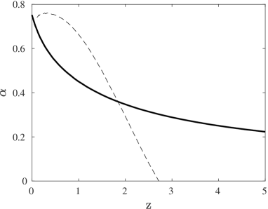
Figure 1.— $\alpha$ (the power-law index of $A_{\rm eff}t_{\rm E}$) as a function of redshift (solid line), assuming Planck cosmological parameters (Planck Collaboration et al. 2016). The solid line represents $\alpha$ in the case of sources with a uniform number per comoving volume, while the dashed line is the approximate $\alpha$ when we introduce the measured evolution in the star formation rate (Cucciati et al. 2012). This plot ignores the evolution in the luminosity function, redshift of the spectrum, and time dilation. For example, the time dilation may be important for transient sources.

We have to be careful not to over interpret this plot. In reality, there are several additional complications. For example, for transient sources (e.g., supernovae), the rate of events further decreases like $1/(1+z)$, due to the time dilation of the transient rate. Moreover, this plot ignores the fact that the luminosity function of sources may change with redshift.

2.6. The source-noise dominated case

So far we have discussed the background-noise dominated regime. For bright sources (e.g., exoplanet transit detection around FGK stars), the source noise is the dominating noise term. The criterion for this case is given by comparing the numerator and the square of the denominator in Equation 1:

$$F_{\rm t}\mathrel{\raise 1.29167pt\hbox{$>$}\mkern-14.0mu\lower 2.58334pt\hbox{$\sim$}}4\pi B\sigma^{2},$$ (14)

where $F_{\rm t}$ is the flux above which the transition from background-noise to source-noise occurs. For example, for $\sigma\approx 0.28^{\prime\prime}$, $1^{\prime\prime}$, $2^{\prime\prime}$, $10^{\prime\prime}$, the transition between background-noise dominated and source-noise dominated occurs at about 0, 2.7, 4.2, and 7.7 magnitudes below the sky surface magnitude (in units of magnitude per square arcseconds), respectively.

In the source-noise-dominated case:

$$\Big{(}\frac{S}{N}\Big{)}=\sqrt{FA_{\rm eff}t_{\rm E}}.$$ (15)

Repeating the steps in §2 with Equation 15 we find

$$\mathcal{G}\propto\Omega\Big{(}\frac{S}{N}\Big{)}^{-3}A_{\rm eff}^{3/2}t_{\rm E}^{3/2}\frac{1}{t_{\rm E}+t_{\rm D}}.$$ (16)

This suggests that deep in the source-noise-dominated case, and for constant $S/N$, larger telescopes are preferable, while the seeing is not important.

2.7. The information-content grasp

For some applications we care about measuring some properties like the flux (e.g., exoplanets search), first moment (e.g., astrometry), or shape (e.g., weak lensing), as precisely as possible. Assuming that we are limited by Poisson noise, we can define the information-content grasp, as the sum of variances of all sources in the field of view.

For sources with a flux density function of the form

$$\frac{dN}{dF}\propto F^{-\zeta},$$ (17)

where $N$ is the number of sources, $F$ is the flux, and $\zeta$ is a power-law index, the volumetric information content integrated between the flux limit ($F_{\rm lim}$) and some upper-flux bound ($F_{\rm max}$; e.g., saturation limit) is

$$V_{\rm I}\propto\Omega\int_{F_{\rm lim}}^{F_{\rm max}}{\Big{(}\frac{S}{N}\Big{)}_{\rm m}^{2}F^{-\zeta}dF}.$$ (18)

Here $(S/N)_{\rm m}^{2}$ is the variance of a measurement process (see general formula in Zackay and Ofek 2017a). For simplicity we will treat only the background dominated case, in which

$$(S/N)_{\rm m}^{2}=\frac{F^{2}}{4\pi\sigma^{2}B}A_{\rm eff}t_{\rm E}.$$ (19)

Note that in the background-noise dominated case, the $S/N$ for detection and measurement are the same. Plugging Equation 19 into Equation 18, setting $x\equiv F_{\rm max}/F_{\rm lim}$, and integrating, we get (for $\zeta\neq 3$) the information-content volume

$$V_{\rm I}=\Omega\frac{(x^{3-\zeta}-1)}{4\pi(\zeta-3)}\frac{A_{\rm eff}t_{\rm E}}{\sigma^{2}B}F_{\rm lim}^{3-\zeta}.$$ (20)

Here $x$ can be regarded as the dynamic range of the observations, and we assume that we are in the background-noise dominated regime in the entire dynamic range. To get the information-content grasp , we plug Equation 2 into Equation 20 and divide by the exposure time plus the dead time.

$$\mathcal{G}_{\rm I}\propto\Omega\frac{(x^{3-\zeta}-1)}{4\pi(\zeta-3)}\Big{(}\frac{S}{N}\Big{)}^{3-\zeta}\sigma^{1-\zeta}\Big{(}\frac{A_{\rm eff}}{B}\Big{)}^{(\zeta-1)/2}\frac{t_{\rm E}^{(\zeta-1)/2}}{t_{\rm E}+t_{\rm D}}.$$ (21)

In the case of an Euclidean Universe with a homogeneous source density ($\zeta=5/2$), and in the background-noise dominated limit, the information-content grasp grows like $\sigma^{-3/2}A_{\rm eff}^{3/4}$. I.e., the information-content grasp scales like the grasp.

3. Telescope cost-effectiveness

We define the cost-effectiveness of a survey telescope as the grasp per unit cost. According to van Belle et al. (2004), the cost of telescopes grows like $\sim A^{\gamma}$, with $\gamma\approx 1.15$, but the exact power-law ranges from $\gamma\approx 1$ to $1.5$, and depends on the telescope details. Furthermore, with newer telescope design, segmented mirrors and shorter focal-ratio implemented in new large telescopes, it is possible that $\gamma$ for large telescopes is slightly smaller than 1. Adopting the basic grasp formula, or even the étendue, suggests that for seeing-dominated survey telescopes, multiple small telescopes have the potential to be more cost-effective than one single large telescope with the same grasp (i.e., $N\Omega_{S}A_{S}^{3/4}=\Omega_{L}A_{L}^{3/4}$; subscripts $S$ and $L$ correspond to small and large telescopes, respectively). For such equivalent systems, the cost-effectiveness of a small telescope system, compared to a large telescope with the same grasp, is proportional to $\sim N(\Omega_{S}/\Omega_{L})(A_{S}/A_{L})^{3/4-\gamma}$. This suggest a factor of a few at most between the cost effectivness of small and large telescopes. It is possible, however, that a larger factor in cost effectivness of small vs. large telescopes hides in mass production, and the use of products which are not unique for professional astronomy.

Given the fast development and progress in detector technology, optics manufacturing technology and computing, as well as the large-scale market economy, when designing a new system, it is worthwhile to compare the capabilities of large vs. small telescopes. This comparison depends on the details of our science goals.

Our rough analysis suggests that the cost-effectiveness of some small telescope systems (e.g., GOTO, Dyer et al. 2018; ATLAS, Tonry 2011, Heinze et al. 2018) is probably higher by a factor of about 3 compared to some of the other small or big survey telescopes. An important question is: Can we further improve the cost effectiveness of telescopes? We argue that technological development of the past several years have likely made it possible to increase the grasp-based cost-effectiveness of seeing-limited imaging survey telescopes by about an order of magnitude. One such development is the fast progress made in the quality of CMOS detectors, which are considerably less expensive than CCD-based cameras, and are available with small pixels (see §4).

4. Practical considerations

In order to maximize the cost-effectiveness of seeing-limited survey telescopes, given the strong dependence of the grasp on the image quality, it is desirable that the system will be limited by the seeing. For a 20 cm telescope, the visible-light diffraction limit is about $0.7^{\prime\prime}$, so our first requirement is for telescopes with a diameter $D\mathrel{\raise 1.29167pt\hbox{$>$}\mkern-14.0mu\lower 2.58334pt\hbox{$\sim$}}20$ cm. Next, we require optics that provide an image quality comparable to the seeing and a pixel size that critically samples the PSF.

Since we would like to maximize the field of view, systems with a short focal length are required. This means that in order to critically sample the PSF, we need small pixels. For example, with a 30 cm f/2 telescope, $3$ $\mu$m pixels are required in order to have a pixel scale of $1^{\prime\prime}$/pix. Most importantly, such large-format back-side illuminated CMOS detectors with small pixels have only now become available. Another important point is that CMOS devices are considerably less expensive than equivalent CCDs, and that CMOS technology is maturing fast. Therefore, utilizing CMOS technology has the potential to further increase the cost-effectiveness of survey telescopes. The pixel-size requirement means that fully utilizing the cost-effectiveness of small telescopes has only recently become possible. Another important factor is that small telescopes and cameras have a huge market, and this has an important impact on their availability, and cost-effectiveness.

The multiple-small-telescopes-for-sky-survey approach has several challenges. First, operating and analyzing data from a large number of telescopes requires considerable computing power and data storage. Saving all the raw data from a large ($\mathcal{O}[1000]$) number of telescopes is challenging. However, a possible solution is to process the data and save selected data products. Second, multiplicity usually comes with some complexity (e.g., maintenance). Therefore, we require a proof that the small telescope approach has the potential to increase the cost-effectiveness, of existing and planned sky-survey systems, by an order of magnitude.

5. Comments about spectroscopy and interferometry

So far we have focused on imaging surveys. It is of interest to consider extending the multiple-small telescope approach to spectroscopy and maybe intensity interferometers (Brown and Twiss 1956, 1957, 1958). Applying this approach to spectroscopy was already discussed in the literature (e.g., Eikenberry et al. 2019).

The grasp formula represents a special case in which we are interested in all, or a subset, of objects in a volume of space. However, in spectroscopy we are typically limited to a fixed number of targets per exposure. Therefore, when discussing spectroscopy, we ignore the gras formula. Nevertheless, it is interesting to understand if constructing a telescope for spectroscopy may be more cost-effective using multiple small telescopes compared to a single telescope with the same collecting area.

Spectroscopic observations using multiple small telescopes requires either a spectrograph per telescope, or combining the light from many telescopes into a single spectrograph (e.g., Eikenberry et al. 2019). Furthermore, one may consider a single object spectrograph, or a multi-object spectrograph. For the spectrograph-per-telescope option, since a single efficient spectrograph may be at least an order of magnitude more expensive than a 20 cm-class telescope, the optimum cost-effective system may require a larger telescope (e.g., 0.5–1 m class). The second option, of efficiently combining the light from multiple small telescopes into a single spectrograph, is challenging. Among the possibilities to combine the light from multiple telescopes is using a variant of the optical multiplexer (Zackay and Gal-Yam 2014, Ben-Ami et al. 2014). Another light-combibibg method was suggested for the PolyOculus project (Eikenberry et al. 2019).

6. Summary

We define the grasp as the relative volume of space that can be observed by a telescope system per unit time (i.e., survey speed). We argue that the grasp of a seeing-limited imaging-survey telescope, even in its simplest form, is a good representation of the scientific return from the system. We derive the grasp formula, and discuss it mainly in the limit of seeing-dominated surveys assuming an Euclidean universe with a uniform source density. We also discuss a related quantity we call the information-content grasp that measures the variance of all sources in the field of view, per unit time.

We argue that, given the power-law dependence of the grasp on the telescope collecting area, combined with recent technological developments, it is now likely more cost-effective to build multiple small telescopes than a single large telescope, with the same grasp and even with the same collecting area. Specifically, the availability of high-quality backside illuminated CMOS devices with small pixels, a large format, and a fast readout may be a game-changer in the near future. Furthermore, these CMOS devices are typically a factor of a few less expensive per unit area, have simpler electronics, and consume less power, compared with the CCD technology. Adopting this approach in astronomy, has the potential to increase the cost-effectiveness of seeing-dominated survey telescopes by an order of magnitude, which eventually may enable faster astronomical research progress. We argue that if all the obstacles to implementing cost-effective wide-field imaging and multi-object spectrographs using multiple small telescopes are removed, then the motivation to build new single large-aperture ($\mathrel{\raise 1.29167pt\hbox{$>$}\mkern-14.0mu\lower 2.58334pt\hbox{$\sim$}}1$ m) visible-light telescopes which are seeing-dominated, will be weakened.

In order to test this ideas we are constructing the the Large-Array Survey Telescope (LAST) project (Ben-Ami et al. in prep.). A LAST node will be constructed from 48, 27-cm f/2.2 telescopes. Each telescope, equipped with a back-side illuminated CMOS device, will have a field of view of about 7.4 deg² and pixel scale of $1.2^{\prime\prime}$. So a LAST node is equivalent to a 27 cm telescope with field-of-view of about 355 deg², or a 1.9 m telescope with field-of-view of 7.4 deg². The goal of the LAST project is not only to conduct scientific investigation, but also to provide a proof-of-concept that it is possible to increase the cost-effectiveness of survey telescopes by an order of magnitude, compared to existing and under-construction systems.

References

- Law et al. (2009) N. M. Law, S. R. Kulkarni, R. G. Dekany, E. O. Ofek, R. M. Quimby, P. E. Nugent, J. Surace, C. C. Grillmair, J. S. Bloom, M. M. Kasliwal, L. Bildsten, T. Brown, S. B. Cenko, D. Ciardi, E. Croner, S. G. Djorgovski, J. van Eyken, A. V. Filippenko, D. B. Fox, A. Gal-Yam, D. Hale, N. Hamam, G. Helou, J. Henning, D. A. Howell, J. Jacobsen, R. Laher, S. Mattingly, D. McKenna, A. Pickles, D. Poznanski, G. Rahmer, A. Rau, W. Rosing, M. Shara, R. Smith, D. Starr, M. Sullivan, V. Velur, R. Walters, and J. Zolkower, PASP 121, 1395 (2009), arXiv:0906.5350 [astro-ph.IM] .
- Chambers et al. (2016) K. C. Chambers, E. A. Magnier, N. Metcalfe, H. A. Flewelling, M. E. Huber, C. Z. Waters, L. Denneau, P. W. Draper, D. Farrow, D. P. Finkbeiner, C. Holmberg, J. Koppenhoefer, P. A. Price, A. Rest, R. P. Saglia, E. F. Schlafly, S. J. Smartt, W. Sweeney, R. J. Wainscoat, W. S. Burgett, S. Chastel, T. Grav, J. N. Heasley, K. W. Hodapp, R. Jedicke, N. Kaiser, R. P. Kudritzki, G. A. Luppino, R. H. Lupton, D. G. Monet, J. S. Morgan, P. M. Onaka, B. Shiao, C. W. Stubbs, J. L. Tonry, R. White, E. Bañados, E. F. Bell, R. Bender, E. J. Bernard, M. Boegner, F. Boffi, M. T. Botticella, A. Calamida, S. Casertano, W. P. Chen, X. Chen, S. Cole, N. Deacon, C. Frenk, A. Fitzsimmons, S. Gezari, V. Gibbs, C. Goessl, T. Goggia, R. Gourgue, B. Goldman, P. Grant, E. K. Grebel, N. C. Hambly, G. Hasinger, A. F. Heavens, T. M. Heckman, R. Henderson, T. Henning, M. Holman, U. Hopp, W. H. Ip, S. Isani, M. Jackson, C. D. Keyes, A. M. Koekemoer, R. Kotak, D. Le, D. Liska, K. S. Long, J. R. Lucey, M. Liu, N. F. Martin, G. Masci, B. McLean, E. Mindel, P. Misra, E. Morganson, D. N. A. Murphy, A. Obaika, G. Narayan, M. A. Nieto-Santisteban, P. Norberg, J. A. Peacock, E. A. Pier, M. Postman, N. Primak, C. Rae, A. Rai, A. Riess, A. Riffeser, H. W. Rix, S. Röser, R. Russel, L. Rutz, E. Schilbach, A. S. B. Schultz, D. Scolnic, L. Strolger, A. Szalay, S. Seitz, E. Small, K. W. Smith, D. R. Soderblom, P. Taylor, R. Thomson, A. N. Taylor, A. R. Thakar, J. Thiel, D. Thilker, D. Unger, Y. Urata, J. Valenti, J. Wagner, T. Walder, F. Walter, S. P. Watters, S. Werner, W. M. Wood-Vasey, and R. Wyse, arXiv e-prints , arXiv:1612.05560 (2016), arXiv:1612.05560 [astro-ph.IM] .
- Gorbovskoy et al. (2013) E. S. Gorbovskoy, V. M. Lipunov, V. G. Kornilov, A. A. Belinski, D. A. Kuvshinov, N. V. Tyurina, A. V. Sankovich, A. V. Krylov, N. I. Shatskiy, P. V. Balanutsa, V. V. Chazov, A. S. Kuznetsov, A. S. Zimnukhov, V. P. Shumkov, S. E. Shurpakov, V. A. Senik, D. V. Gareeva, M. V. Pruzhinskaya, A. G. Tlatov, A. V. Parkhomenko, D. V. Dormidontov, V. V. Krushinsky, A. F. Punanova, I. S. Zalozhnyh, A. A. Popov, A. Y. Burdanov, S. A. Yazev, N. M. Budnev, K. I. Ivanov, E. N. Konstantinov, O. A. Gress, O. V. Chuvalaev, V. V. Yurkov, Y. P. Sergienko, I. V. Kudelina, E. V. Sinyakov, I. D. Karachentsev, A. V. Moiseev, and T. A. Fatkhullin, Astronomy Reports 57, 233 (2013), arXiv:1305.1620 [astro-ph.HE] .
- Kochanek et al. (2017) C. S. Kochanek, B. J. Shappee, K. Z. Stanek, T. W. S. Holoien, T. A. Thompson, J. L. Prieto, S. Dong, J. V. Shields, D. Will, C. Britt, D. Perzanowski, and G. Pojmański, PASP 129, 104502 (2017), arXiv:1706.07060 [astro-ph.SR] .
- Dyer et al. (2018) M. J. Dyer, V. S. Dhillon, S. Littlefair, D. Steeghs, K. Ulaczyk, P. Chote, D. Galloway, and E. Rol, in Proc. SPIE, Society of Photo-Optical Instrumentation Engineers (SPIE) Conference Series, Vol. 10704 (2018) p. 107040C, arXiv:1807.01614 [astro-ph.IM] .
- Bellm et al. (2019a) E. C. Bellm, S. R. Kulkarni, M. J. Graham, R. Dekany, R. M. Smith, R. Riddle, F. J. Masci, G. Helou, T. A. Prince, and S. M. Adams, PASP 131, 018002 (2019a), arXiv:1902.01932 [astro-ph.IM] .
- Tyson et al. (2001) J. A. Tyson, D. M. Wittman, and J. R. P. Angel, in Gravitational Lensing: Recent Progress and Future Go, Astronomical Society of the Pacific Conference Series, Vol. 237, edited by T. G. Brainerd and C. S. Kochanek (2001) p. 417, arXiv:astro-ph/0005381 [astro-ph] .
- Abbott et al. (2017) B. P. Abbott, R. Abbott, T. D. Abbott, F. Acernese, K. Ackley, C. Adams, T. Adams, P. Addesso, R. X. Adhikari, and V. B. Adya, Phys. Rev. Lett. 119, 161101 (2017), arXiv:1710.05832 [gr-qc] .
- Cenko et al. (2013) S. B. Cenko, S. R. Kulkarni, A. Horesh, A. Corsi, D. B. Fox, J. Carpenter, D. A. Frail, P. E. Nugent, D. A. Perley, and D. Gruber, ApJ 769, 130 (2013), arXiv:1304.4236 [astro-ph.CO] .
- Charbonneau et al. (2000) D. Charbonneau, T. M. Brown, D. W. Latham, and M. Mayor, ApJ 529, L45 (2000), arXiv:astro-ph/9911436 [astro-ph] .
- Nutzman and Charbonneau (2008) P. Nutzman and D. Charbonneau, PASP 120, 317 (2008), arXiv:0709.2879 [astro-ph] .
- Swift et al. (2015) J. J. Swift, M. Bottom, J. A. Johnson, J. T. Wright, N. McCrady, R. A. Wittenmyer, P. Plavchan, R. Riddle, P. S. Muirhead, E. Herzig, J. Myles, C. H. Blake, J. Eastman, T. G. Beatty, S. I. Barnes, S. R. Gibson, B. Lin, M. Zhao, P. Gardner, E. Falco, S. Criswell, C. Nava, C. Robinson, D. H. Sliski, R. Hedrick, K. Ivarsen, A. Hjelstrom, J. de Vera, and A. Szentgyorgyi, Journal of Astronomical Telescopes, Instruments, and Systems 1, 027002 (2015), arXiv:1411.3724 [astro-ph.IM] .
- Tonry (2011) J. L. Tonry, PASP 123, 58 (2011), arXiv:1011.1028 [astro-ph.IM] .
- Djorgovski et al. (2012) S. G. Djorgovski, A. A. Mahabal, A. J. Drake, M. J. Graham, C. Donalek, and R. Williams, in New Horizons in Time Domain Astronomy, IAU Symposium, Vol. 285, edited by E. Griffin, R. Hanisch, and R. Seaman (2012) pp. 141–146, arXiv:1111.2078 [astro-ph.IM] .
- Pepper et al. (2002) J. Pepper, A. Gould, and D. L. DePoy, arXiv e-prints , astro-ph/0209310 (2002), arXiv:astro-ph/0209310 [astro-ph] .
- Bellm (2016) E. C. Bellm, PASP 128, 084501 (2016), arXiv:1605.02081 [astro-ph.IM] .
- Bakos et al. (2004) G. Bakos, R. W. Noyes, G. Kovács, K. Z. Stanek, D. D. Sasselov, and I. Domsa, PASP 116, 266 (2004), arXiv:astro-ph/0401219 [astro-ph] .
- Pollacco et al. (2006) D. L. Pollacco, I. Skillen, A. Collier Cameron, D. J. Christian, C. Hellier, J. Irwin, T. A. Lister, R. A. Street, R. G. West, D. R. Anderson, W. I. Clarkson, H. Deeg, B. Enoch, A. Evans, A. Fitzsimmons, C. A. Haswell, S. Hodgkin, K. Horne, S. R. Kane, F. P. Keenan, P. F. L. Maxted, A. J. Norton, J. Osborne, N. R. Parley, R. S. I. Ryans, B. Smalley, P. J. Wheatley, and D. M. Wilson, PASP 118, 1407 (2006), arXiv:astro-ph/0608454 [astro-ph] .
- Law et al. (2015) N. M. Law, O. Fors, J. Ratzloff, P. Wulfken, D. Kavanaugh, D. J. Sitar, Z. Pruett, M. N. Birchard, B. N. Barlow, K. Cannon, S. B. Cenko, B. Dunlap, A. Kraus, and T. J. Maccarone, PASP 127, 234 (2015), arXiv:1501.03162 [astro-ph.IM] .
- Wheatley et al. (2018) P. J. Wheatley, R. G. West, M. R. Goad, J. S. Jenkins, D. L. Pollacco, D. Queloz, H. Rauer, S. Udry, C. A. Watson, B. Chazelas, P. Eigmüller, G. Lambert, L. Genolet, J. McCormac, S. Walker, D. J. Armstrong, D. Bayliss, J. Bento, F. Bouchy, M. R. Burleigh, J. Cabrera, S. L. Casewell, A. Chaushev, P. Chote, S. Csizmadia, A. Erikson, F. Faedi, E. Foxell, B. T. Gänsicke, E. Gillen, A. Grange, M. N. Günther, S. T. Hodgkin, J. Jackman, A. Jordán, T. Louden, L. Metrailler, M. Moyano, L. D. Nielsen, H. P. Osborn, K. Poppenhaeger, R. Raddi, L. Raynard, A. M. S. Smith, M. Soto, and R. Titz-Weider, MNRAS 475, 4476 (2018), arXiv:1710.11100 [astro-ph.EP] .
- Heinze et al. (2018) A. N. Heinze, J. L. Tonry, L. Denneau, H. Flewelling, B. Stalder, A. Rest, K. W. Smith, S. J. Smartt, and H. Weiland, AJ 156, 241 (2018), arXiv:1804.02132 [astro-ph.SR] .
- Abraham and van Dokkum (2014) R. G. Abraham and P. G. van Dokkum, PASP 126, 55 (2014), arXiv:1401.5473 [astro-ph.IM] .
- Danieli et al. (2018) S. Danieli, P. van Dokkum, and C. Conroy, ApJ 856, 69 (2018), arXiv:1711.00860 [astro-ph.GA] .
- Bellm et al. (2019b) E. C. Bellm, S. R. Kulkarni, T. Barlow, U. Feindt, M. J. Graham, A. Goobar, T. Kupfer, C.-C. Ngeow, P. Nugent, and E. Ofek, PASP 131, 068003 (2019b), arXiv:1905.02209 [astro-ph.IM] .
- Zackay and Ofek (2017a) B. Zackay and E. O. Ofek, ApJ 836, 187 (2017a), arXiv:1512.06872 [astro-ph.IM] .
- Nir et al. (2019) G. Nir, B. Zackay, and E. O. Ofek, AJ 158, 70 (2019), arXiv:1809.09933 [astro-ph.IM] .
- Labeyrie (1970) A. Labeyrie, A&A 6, 85 (1970).
- Bates (1982) R. H. T. Bates, Phys. Rep. 90, 203 (1982).
- Zackay and Ofek (2017b) B. Zackay and E. O. Ofek, ApJ 836, 188 (2017b), arXiv:1512.06879 [astro-ph.IM] .
- Ratzloff et al. (2019) J. K. Ratzloff, N. M. Law, O. Fors, H. T. Corbett, W. S. Howard, D. del Ser, and J. Haislip, PASP 131, 075001 (2019), arXiv:1904.11991 [astro-ph.IM] .
- Cucciati et al. (2012) O. Cucciati, L. Tresse, O. Ilbert, O. Le Fèvre, B. Garilli, V. Le Brun, P. Cassata, P. Franzetti, D. Maccagni, M. Scodeggio, E. Zucca, G. Zamorani, S. Bardelli, M. Bolzonella, R. M. Bielby, H. J. McCracken, A. Zanichelli, and D. Vergani, A&A 539, A31 (2012), arXiv:1109.1005 [astro-ph.CO] .
- Planck Collaboration et al. (2016) Planck Collaboration, P. A. R. Ade, N. Aghanim, M. Arnaud, M. Ashdown, J. Aumont, C. Baccigalupi, A. J. Banday, R. B. Barreiro, J. G. Bartlett, N. Bartolo, E. Battaner, R. Battye, K. Benabed, A. Benoît, A. Benoit-Lévy, J. P. Bernard, M. Bersanelli, P. Bielewicz, J. J. Bock, A. Bonaldi, L. Bonavera, J. R. Bond, J. Borrill, F. R. Bouchet, F. Boulanger, M. Bucher, C. Burigana, R. C. Butler, E. Calabrese, J. F. Cardoso, A. Catalano, A. Challinor, A. Chamballu, R. R. Chary, H. C. Chiang, J. Chluba, P. R. Christensen, S. Church, D. L. Clements, S. Colombi, L. P. L. Colombo, C. Combet, A. Coulais, B. P. Crill, A. Curto, F. Cuttaia, L. Danese, R. D. Davies, R. J. Davis, P. de Bernardis, A. de Rosa, G. de Zotti, J. Delabrouille, F. X. Désert, E. Di Valentino, C. Dickinson, J. M. Diego, K. Dolag, H. Dole, S. Donzelli, O. Doré, M. Douspis, A. Ducout, J. Dunkley, X. Dupac, G. Efstathiou, F. Elsner, T. A. Enßlin, H. K. Eriksen, M. Farhang, J. Fergusson, F. Finelli, O. Forni, M. Frailis, A. A. Fraisse, E. Franceschi, A. Frejsel, S. Galeotta, S. Galli, K. Ganga, C. Gauthier, M. Gerbino, T. Ghosh, M. Giard, Y. Giraud-Héraud, E. Giusarma, E. Gjerløw, J. González-Nuevo, K. M. Górski, S. Gratton, A. Gregorio, A. Gruppuso, J. E. Gudmundsson, J. Hamann, F. K. Hansen, D. Hanson, D. L. Harrison, G. Helou, S. Henrot-Versillé, C. Hernández-Monteagudo, D. Herranz, S. R. Hildebrand t, E. Hivon, M. Hobson, W. A. Holmes, A. Hornstrup, W. Hovest, Z. Huang, K. M. Huffenberger, G. Hurier, A. H. Jaffe, T. R. Jaffe, W. C. Jones, M. Juvela, E. Keihänen, R. Keskitalo, T. S. Kisner, R. Kneissl, J. Knoche, L. Knox, M. Kunz, H. Kurki-Suonio, G. Lagache, A. Lähteenmäki, J. M. Lamarre, A. Lasenby, M. Lattanzi, C. R. Lawrence, J. P. Leahy, R. Leonardi, J. Lesgourgues, F. Levrier, A. Lewis, M. Liguori, P. B. Lilje, M. Linden-Vørnle, M. López-Caniego, P. M. Lubin, J. F. Macías-Pérez, G. Maggio, D. Maino, N. Mandolesi, A. Mangilli, A. Marchini, M. Maris, P. G. Martin, M. Martinelli, E. Martínez-González, S. Masi, S. Matarrese, P. McGehee, P. R. Meinhold, A. Melchiorri, J. B. Melin, L. Mendes, A. Mennella, M. Migliaccio, M. Millea, S. Mitra, M. A. Miville-Deschênes, A. Moneti, L. Montier, G. Morgante, D. Mortlock, A. Moss, D. Munshi, J. A. Murphy, P. Naselsky, F. Nati, P. Natoli, C. B. Netterfield, H. U. Nørgaard-Nielsen, F. Noviello, D. Novikov, I. Novikov, C. A. Oxborrow, F. Paci, L. Pagano, F. Pajot, R. Paladini, D. Paoletti, B. Partridge, F. Pasian, G. Patanchon, T. J. Pearson, O. Perdereau, L. Perotto, F. Perrotta, V. Pettorino, F. Piacentini, M. Piat, E. Pierpaoli, D. Pietrobon, S. Plaszczynski, E. Pointecouteau, G. Polenta, L. Popa, G. W. Pratt, G. Prézeau, S. Prunet, J. L. Puget, J. P. Rachen, W. T. Reach, R. Rebolo, M. Reinecke, M. Remazeilles, C. Renault, A. Renzi, I. Ristorcelli, G. Rocha, C. Rosset, M. Rossetti, G. Roudier, B. Rouillé d’Orfeuil, M. Rowan-Robinson, J. A. Rubiño-Martín, B. Rusholme, N. Said, V. Salvatelli, L. Salvati, M. Sandri, D. Santos, M. Savelainen, G. Savini, D. Scott, M. D. Seiffert, P. Serra, E. P. S. Shellard, L. D. Spencer, M. Spinelli, V. Stolyarov, R. Stompor, R. Sudiwala, R. Sunyaev, D. Sutton, A. S. Suur-Uski, J. F. Sygnet, J. A. Tauber, L. Terenzi, L. Toffolatti, M. Tomasi, M. Tristram, T. Trombetti, M. Tucci, J. Tuovinen, M. Türler, G. Umana, L. Valenziano, J. Valiviita, F. Van Tent, P. Vielva, F. Villa, L. A. Wade, B. D. Wandelt, I. K. Wehus, M. White, S. D. M. White, A. Wilkinson, D. Yvon, A. Zacchei, and A. Zonca, A&A 594, A13 (2016), arXiv:1502.01589 [astro-ph.CO] .
- van Belle et al. (2004) G. T. van Belle, A. B. Meinel, and M. P. Meinel, in Proc. SPIE, Society of Photo-Optical Instrumentation Engineers (SPIE) Conference Series, Vol. 5489, edited by J. Oschmann, Jacobus M. (2004) pp. 563–570.
- Martinez et al. (2010) P. Martinez, J. Kolb, M. Sarazin, and A. Tokovinin, The Messenger 141, 5 (2010).
- Ofek (2019) E. O. Ofek, PASP 131, 054504 (2019), arXiv:1903.02015 [astro-ph.IM] .
- Brown and Twiss (1956) R. H. Brown and R. Q. Twiss, Nature 177, 27 (1956).
- Brown and Twiss (1957) R. H. Brown and R. Q. Twiss, Proceedings of the Royal Society of London Series A 242, 300 (1957).
- Brown and Twiss (1958) R. H. Brown and R. Q. Twiss, Proceedings of the Royal Society of London Series A 248, 199 (1958).
- Eikenberry et al. (2019) S. S. Eikenberry, M. Bentz, A. Gonzalez, J. Harrington, S. Jeram, N. Law, T. Maccarone, R. Quimby, and A. Townsend, arXiv e-prints , arXiv:1907.08273 (2019), arXiv:1907.08273 [astro-ph.IM] .
- Zackay and Gal-Yam (2014) B. Zackay and A. Gal-Yam, PASP 126, 148 (2014), arXiv:1310.3714 [astro-ph.IM] .
- Ben-Ami et al. (2014) S. Ben-Ami, B. Zackay, A. Rubin, I. Sagiv, A. Gal-Yam, and E. O. Ofek, in Proc. SPIE, Society of Photo-Optical Instrumentation Engineers (SPIE) Conference Series, Vol. 9147 (2014) p. 91475U.