C³ - Cluster Clustering Cosmology
II. First detection of the BAO peak in the three-point correlation function of galaxy clusters

Abstract

Third-order statistics of the cosmic density field provides a powerful cosmological probe containing synergistic information to the more commonly explored second-order statistics. Here, we exploit a spectroscopic catalog of 72,563 clusters of galaxies extracted from the Sloan Digital Sky Survey, providing the first detection of the baryon acoustic oscillations (BAO) peak in the three-point correlation function (3PCF) of galaxy clusters. We measure and analyze both the connected and the reduced 3PCF of SDSS clusters from intermediate ($r\sim 10$ Mpc/h) up to large ($r\sim 140$ Mpc/h) scales, exploring a variety of different configurations. From the analysis of reduced 3PCF at intermediate scales, in combination with the analysis of the two-point correlation function, we constrain both the cluster linear and non-linear bias parameters, $b_{1}=2.75\pm 0.03$ and $b_{2}=1.2\pm 0.5$. We analyze the measurements of the 3PCF at larger scales, comparing them with theoretical models. The data show clear evidence of the BAO peak in different configurations, which appears more visible in the reduced 3PCF rather than in the connected one. From the comparison between theoretical models considering or not the BAO peak, we obtain a quantitative estimate of this evidence, with a $\Delta\chi^{2}$ between 2 and 75, depending on the considered configuration. Finally, we set up a generic framework to estimate the expected signal-to-noise ratio of the BAO peak in the 3PCF exploring different possible definitions, that can be used to forecast the most favorable configurations to be explored also in different future surveys, and applied it to the case of the Euclid mission.

1 Introduction

Since the discovery of the accelerated expansion of the Universe (Riess et al., 1998; Perlmutter et al., 1999), two main issues have been the focus of modern cosmology: what are the main components of our Universe, and how the Universe evolves. These questions involve the understanding of both the geometry of our Universe and its evolution. To address these issues many different cosmological probes have been introduced and studied in the last twenty years; for a complete review, we refer to the recent work by Huterer & Shafer (2018).

In recent years, the study of the clustering of large scale structures has rapidly become one of the main cosmological probes, because it retains cosmological information of the primordial Universe in the form of peculiar matter overdensities that appear around 100 $h^{-1}$ Mpc, as initially predicted in the seminal works of Sunyaev & Zeldovich (1970) and Peebles & Yu (1970). These features are called baryon acoustic oscillations (BAO), and can be used as standard rulers to constrain the expansion history of the Universe. In Fourier space, they appear as wiggles in the power spectrum, $P(k)$, while in configuration space as a distinctive peak around $r\sim$ 100 $h^{-1}$ Mpc in the two-point correlation function (2PCF).

After the first BAO measurements by Eisenstein et al. (2005) and Cole et al. (2005), several works followed, exploring in detail the cosmological constraining power of BAO (Percival et al., 2007; Blake et al., 2011; Beutler et al., 2011; Padmanabhan et al., 2012; Anderson et al., 2014; Ross et al., 2015; Alam et al., 2017; Bautista et al., 2020; Gil-Marín et al., 2020), leading to several surveys and space missions that are currently being developed aiming at pushing the accuracy of this probe down to the percentage level, like Euclid (Laureijs et al., 2011), the Vera C. Rubin Observatory LSST (Ivezić et al., 2019), and the Nancy Grace Roman Space Telescope (Spergel et al., 2015).

As a parallel effort to the study of two-point statistics, increasingly more attention is being given to higher-order correlation functions, and in particular to the three-point statistics, namely the three-point correlation function (3PCF) in configuration space, and its analogous in Fourier space, the bispectrum $B(k)$. Pioneering studies on the 3PCF can be traced back to the late seventies (Peebles & Groth, 1975; Groth & Peebles, 1977). Historically, the 3PCF has been mainly exploited to characterize extra-galactic samples in terms of their spatial distribution as a function of properties such as luminosity or stellar mass (Fry, 1994; Frieman & Gaztanaga, 1994; Jing et al., 1995; Jing & Börner, 1998, 2004; Kayo et al., 2004; Gaztañaga & Scoccimarro, 2005; Nichol et al., 2006; Kulkarni et al., 2007; McBride et al., 2011; Marín, 2011; Guo et al., 2014, 2015, 2016; Moresco et al., 2017), while in recent years it has been used also to place constraints on the evolution of some parameters, such as the sample bias or the matter power spectrum normalization, $\sigma_{8}$, as a function of redshift (Marín et al., 2013; Moresco et al., 2014; Hoffmann et al., 2015). For more extensive reviews on the topic, we refer to Bernardeau et al. (2002), Takada & Jain (2003), and Desjacques et al. (2018).

Studies on the exploitation of the 3PCF for cosmological purposes, and in particular to detect and constrain BAO, are, instead, scarcer. The first detection of the BAO peak in the 3PCF is provided by Gaztañaga et al. (2009) from the analysis of Sloan Digital Sky Survey (SDSS) Data Release 7 (DR7) Luminous Red Galaxies. More recently, Slepian et al. (2017a, b) obtained a clear detection of the BAO feature in the 3PCF of SDSS-DR12 CMASS sample, while de Carvalho et al. (2020) measured the BAO feature in the angular 3PCF of SDSS-DR12 quasars.

In this work, we present the first significant detection of the BAO peak in the 3PCF of galaxy clusters. Clusters of galaxies represent the most massive virialized systems in our Universe, with masses $\log(M/M_{\odot})\gtrsim 14$, and comprising up to thousands of galaxies. These systems are extremely important laboratories both from astrophysical and cosmological points of view; in this latter context, they have been used to study the properties of dark energy, since their number density can directly provide constraints on the underlying cosmology (e.g. Vikhlinin et al., 2009; Pacaud et al., 2018; Costanzi et al., 2019; Lesci et al., in prep.). This topic has been extensively studied both in simulations and observations, so that the cluster number counts currently represent a key additional cosmological probe (for a detailed review on this topic, we refer to Allen et al., 2011). The properties of galaxy clusters make them ideal to be studied also from a clustering perspective. Being extremely massive systems, they are characterized by a large bias, and therefore the clustering signal is stronger compared to a galaxy sample with comparable, or also larger densities. Moreover, the effects of non-linear dynamics have a smaller impact on cluster than on field galaxies, with a resulting smaller systematic effect due to redshift-space distortions (RSD) (Valageas & Clerc, 2012; Marulli et al., 2017). For these reasons, galaxy clusters have been extensively analyzed in terms of two-point statistics (e.g. Estrada et al., 2009; Hütsi, 2010; Hong et al., 2012; Veropalumbo et al., 2014, 2016; Sereno et al., 2015; Hong et al., 2016; Marulli et al., 2018, 2020; Nanni et al., in prep.), while the analyses on higher-orders are significantly less developed.

This work is part of a project called “Cluster Clustering Cosmology ($C^{3}$)” where we exploit the constraining power of cluster clustering. In Paper I (Marulli et al., 2020) we analyze the RSD of galaxy clusters, providing a new strong constraint on the product between the linear growth rate of cosmic structures $f$ and the amplitude of linear matter density fluctuations quantified at 8 $h^{-1}\,\mbox{Mpc}$ $\sigma_{8}$ at an effective redshift $z\sim 0.3$, $f\sigma_{8}=0.46\pm 0.03$. In Paper III (Veropalumbo et al., in prep.), we explore the combination of 2PCF and 3PCF in a joint analysis of RSD and BAO.

This paper is organized as follows. In Sect. 2 we give an overview of the methods adopted in this analysis, presenting the estimators used to measure the 3PCF, the models considered, and the code developed to perform the measurements and the statistical analysis. In Sect. 3 we present the cluster catalog used in this analysis. In Sect. 4 we discuss the 3PCF measurements performed, how they have been analyzed to extract information on the bias parameters of the sample, and the advantage of using clusters as opposed to normal galaxies as tracers. Then in Sect. 5 we focus on the BAO peak in the measured 3PCF, quantifying the statistical level of the detection. In Sect. 6 we introduce a framework to forecast the expected signal-to-noise ratio (SNR) of the BAO peak in the 3PCF, focusing on two possible methods, one model-dependent and one model-independent, to identify the peak, and apply them to provide forecasts for the Euclid mission, discussing the constraining potential of the 3PCF as a function of methods and configurations. Finally, in Sect. 7, we draw our conclusions.

Throughout this paper, we assume a Planck18 cosmology (Planck Collaboration et al., 2018) when otherwise explicitly stated, with $\Omega_{\rm m}=0.3153$, $\Omega_{\rm DE}=0.684607$, and $\rm H_{0}=67.36$ km/s/Mpc.

2 Methods

2.1 Definitions

Given a generic spatial distribution of objects, the 3PCF is defined as the statistical function that provides the probability of finding triplets of objects at corresponding comoving separations $r_{12}$, $r_{13}$, and $r_{23}$ (Peebles, 1980). Specifically, the 3PCF $\zeta$ can be defined implicitly as follows:

$$d{\rm P}=\bar{n}^{3}[1+\xi(r_{12})+\xi(r_{13})+\xi(r_{23})+\zeta(r_{12},r_{13},r_{23})]\\ dV_{1}dV_{2}dV_{3}\,,$$ (1)

where $\bar{n}$ is the average density of the objects, $V_{i}$ the comoving volumes at $\overrightarrow{r_{i}}$, and $\xi$ is the 2PCF of the sample at comoving separations ${r_{ij}}$.

While several estimators have been proposed to compute the 2PCF (e.g. Peebles & Hauser, 1974; Hewett, 1982; Davis & Peebles, 1983; Landy & Szalay, 1993; Hamilton, 1993; Keihänen et al., 2019), fewer studies have been performed so far for the 3PCF (e.g., Jing & Börner, 1998; Szapudi & Szalay, 1998; Sosa Nuñez & Niz, 2020). Here we will exploit the widely used formulation proposed by Szapudi & Szalay (1998), that provides an unbiased and with minimal variance estimator based on the counting of triplets between the input catalog (that we will label as data catalog, $D$), and a corresponding random catalog (that we will label as $R$), constructed to reproduce the geometric distribution of the input catalog, but with zero clustering. Specifically, the Szapudi & Szalay (1998) estimator is constructed as follows:

$$\zeta(r_{12},r_{13},r_{23})=\frac{DDD-3DDR+3DRR-RRR}{RRR}\,,$$ (2)

where $DDD$, $RRR$, $DDR$, and $DRR$ are the triplets having comoving separations $(r_{12},r_{13},r_{23})$ in the data catalog, in the random catalog, and in the mixed data-random catalogs, normalized by $N^{3}_{D}/6$, $N^{3}_{R}/6$, $N^{2}_{D}N_{R}/2$, and $N_{D}N^{2}_{R}/2$, respectively.

With a similar approach, Landy & Szalay (1993) have defined an estimator for the 2PCF, $\xi(r)$, based on pair counting in the data and random catalogs:

$$\xi(r)=\frac{DD-2DR+RR}{RR}\,,$$ (3)

where $DD$, $RR$, and $DR$ are the pairs having a comoving separation $r$ in the data catalog, in the random catalog, and in the mixed one, normalized by $N^{2}_{D}/2$, $N^{2}_{R}/2$, and $N_{D}N_{R}$, respectively.

Since it can be demonstrated that in hierarchical scenarios the connected 3PCF, $\zeta$, is proportional to $\xi^{2}$ (Peebles & Groth, 1975), a natural quantity that can be derived is the reduced 3PCF, $Q$ (Groth & Peebles, 1977), defined as:

$$Q(r_{12},r_{13},r_{23})\equiv\frac{\zeta(r_{12},r_{13},r_{23})}{\xi(r_{12})\xi(r_{13})+\xi(r_{13})\xi(r_{23})+\xi(r_{23})\xi(r_{13})}\,.$$ (4)

This new quantity is particularly convenient because it is characterized by a smaller variation of its values as a function of scales. Its values are, by definition, close to unity at all scales, differently from $\zeta$ that may vary by over three orders of magnitude from small to intermediate scales. A further advantage is that it does not depend on $\sigma_{8}$ (unlike the 2PCF or the connected 3PCF), but only on the bias parameters (see Sect. 2.2).

Several parameterizations of triangle shapes have been proposed in the literature to study the 3PCF. Usually, they involve the definition of two sides of the triangle, exploring the dependence of the 3PCF on the third side (Jing et al., 1995; Gaztañaga & Scoccimarro, 2005; Nichol et al., 2006; Kulkarni et al., 2007; Guo et al., 2014). Alternatively, it might be convenient to fix all sides of the triangles (typically in an equilateral configuration) and to analyze the 3PCF at increasing scales (see e.g. Wang et al., 2004; Fosalba et al., 2005; Marín et al., 2008), or to follow an approach similar to the one adopted for the bispectrum and to study the 3PCF at all scales (see e.g. Veropalumbo et al., in prep.). Here, we follow the parameterization proposed by Marín (2011), in which the first two sides of the triangle are fixed, one as a function of the other $r_{13}=u\times r_{12}$, and the 3PCF is calculated either as a function of the third side, or of the angle $\theta$ between the two sides:

$$\left\{\begin{array}[]{l}r_{12}\\ r_{13}=u\cdot r_{12}\\ r_{23}\equiv r_{12}\cdot\sqrt{1+u^{2}-2\cdot u\cdot\cos\theta}\,.\end{array}\right.$$

In this approach, configurations with either $\theta\sim 0$ or $\theta\sim\pi$ will represent the elongated configurations, while the ones with $\theta\sim\pi/2$ represent the isosceles configurations.

2.2 The models

The real-space overdensity of galaxy clusters, $\delta_{c}$, can be expressed with a perturbative expansion as a function of the dark-matter one, $\delta_{m}$, as follows (Fry & Gaztanaga, 1993):

$$\delta_{c}\approx b_{1}\delta_{m}+\frac{b_{2}}{2}\left(\delta^{2}_{m}-<\delta^{2}_{m}>\right)\,.$$ (5)

This equation, known as the local bias approximation, relates the clusters and dark matter overdensities as a function of two parameters, the linear bias $b_{1}$ and the non-linear bias $b_{2}$, neglecting a possible tidal tensor bias contribution.

Using this approximation, it is possible to express also the 2PCF and the 3PCF of clusters as a function of the dark-matter one as follows:

$$\xi_{c} = \left(\frac{\sigma_{8}}{\sigma_{8,fid}}\right)^{2}b_{1}\xi_{m}$$

$$\zeta_{c} = \left(\frac{\sigma_{8}}{\sigma_{8,fid}}\right)^{4}\left[b_{1}^{3}\zeta_{m}+b_{2}b_{1}^{2}\left(\xi_{m}(r_{12})\xi_{m}(r_{12})\right)+perm\right]$$

$$Q_{c} = \frac{1}{b_{1}}\left(Q_{m}+\frac{b_{1}}{b_{2}}\right)\,,$$ (6)

where $\sigma_{8,fid}$ is the amplitude of linear matter density fluctuations quantified at 8 $h^{-1}\,\mbox{Mpc}$ for the fiducial model.

As it can be inferred from the previous equations, the effect of the bias parameters in both $\xi$ and $\zeta$ is degenerate with $\sigma_{8}$, differently from the reduced 3PCF case. More recently, Bel et al. (2015) proposed also an extension of Eq. (6) which includes also the tidal tensor bias $g_{2}$:

$$Q_{c}=\frac{1}{b_{1}}\left(Q_{m}+\frac{b_{1}}{b_{2}}+g_{2}\;Q_{non-loc}\right)\,,$$ (7)

where $Q_{non-loc}$ is the non-local contribution to the 3PCF.

2.3 The code

The theoretical and observational data computed in this analysis have been obtained using the CosmoBolognaLib suite (hereafter CBL, Marulli et al., 2016), which is a public C++ and Python library for cosmological measurements. Originally, the CBL library provided the basic functions to perform measurements of the 2PCF and 3PCF in a variety of possible configurations, to model the 2PCF and perform cosmological computations. The core function of the library, which allows to significantly reduce the computation time for both of the correlation functions, is a chain-mesh (also known as linked-list) approach, which indicizes the particles depending on their spatial position, then looping only on the particles that actually contribute to the counts of pairs and triplets for the considered separations.

Since then, the library has been significantly expanded with additional functionalities. Among them, e.g., significant work on void detection and modelization has been done, including new functions to detect, count, and model cosmic void statistics (Ronconi & Marulli, 2017; Contarini et al., 2019; Ronconi et al., 2019). Moreover, new modules have been added for improved 2PCF modeling (García-Farieta et al., 2020).

For the purpose of this analysis, the CBL library has been significantly updated, with respect to the previous releases, to include new features related to both the analysis and theoretical modelization of the 3PCF. In particular, the chain-mesh approach has been improved with a new method to save triplets during their counting that allows a fast computation of errors based on either jack-knife (JK) or bootstrap (BS) approaches. More recently, Slepian & Eisenstein (2015) proposed an alternative method to calculate the 3PCF, based on a spherical harmonics expansion that skips the direct estimation of the number of triplets in a given configuration, thus significantly reducing the computational time, at the price of a smaller accuracy for the isosceles configurations. This method has been added also in the CBL library, so that the user can choose if estimating the 3PCF either with the direct-counting method or with the spherical-harmonics-decomposition approach.

Two different 3PCF theoretical models have been also implemented, both for connected and reduced 3PCFs, taken from Barriga & Gaztañaga (2002) and Slepian & Eisenstein (2015). These models are obtained as the anti-Fourier transform of the real-space tree-level halo bispectrum. For symmetry reasons, this transformation reduces to a combination of 1D integrals of the linear power spectrum. Slepian et al. (2017b) used a similar approach to derive the three-point correlation function model from the tree-level redshift-space bispectrum. A theoretical estimate of the covariance matrix for $\zeta$, which assumes a Gaussian Random Field density and a boundary-free survey, has also been added to the library, as proposed by Slepian & Eisenstein (2015). Finally, different models to estimate bias parameters have also been included (see Sect. 4). All these new functions are fully documented in the official web-page of the project.

3 Data

The galaxy cluster sample used in this analysis has been obtained with the same procedure discussed by Veropalumbo et al. (2016), that is from a cross-correlation between the photometric cluster catalog provided by Wen et al. (2012) and the spectroscopic redshifts available from the SDSS Data Release 12 (DR12), considering both the Main Galaxy Sample (MGS) and BOSS surveys.

The parent catalog comprises 132,684 clusters extracted from SDSS-III between $0.05\leq z<0.8$; these clusters have been selected from the photometric galaxy catalog, over $\sim 14,000$ square degrees of the SDSS, with an improved version of the Friend-of-Friend algorithm (Huchra & Geller, 1982). The obtained sample is characterized by a richness $R_{L*}>12$, and more than eight member candidates within $r_{200}$, with typical masses larger than $M_{200}/M_{\odot}>6\times 10^{13}$, where $r_{200}$ and $M_{200}$ are, respectively, the radius within which the mean density of the cluster is 200 times larger than the critical density of the Universe at the cluster redshift, and the mass enclosed within $r_{200}$.

This catalog has been cross-correlated with the spectroscopic redshift information available in SDSS-DR12 (Dawson et al., 2013; Alam et al., 2015, 2017), with a significantly increased accuracy in the determination of the position of the galaxies with respect to the photometric ones ($\sigma_{z}/z\sim 0.001$ instead of $\sigma_{z}/z\sim 0.03$), which is proven to be fundamental for clustering measurements. This procedure assigns to each cluster the spectroscopic redshift of its brightest central galaxy (BCG), when available.

The final sample comprises 72,563 galaxy clusters in the redshift range $0.1<z<0.7$. The mean redshift is $<z>=0.38$. Their angular position and redshift distributions are shown in Fig. 1.

An associated random catalog has been built following the same approach used in the BOSS collaboration (Reid et al., 2016). The MANGLE code (Swanson et al., 2008) has been used to track the coordinates of our sample following the spectroscopic tiles of the survey. A Gaussian kernel of $\sigma_{z}=0.02$ has then been used to smooth the redshift distribution. We verified that this assumption does not have a significant impact on the final results. The random catalog has been extracted with a number of objects $N_{R}=50\times N_{D}$, to significantly reduce the shot-noise contribution to the final error budget. For more details, we refer to Veropalumbo et al. (2016) and Marulli et al. (2020).

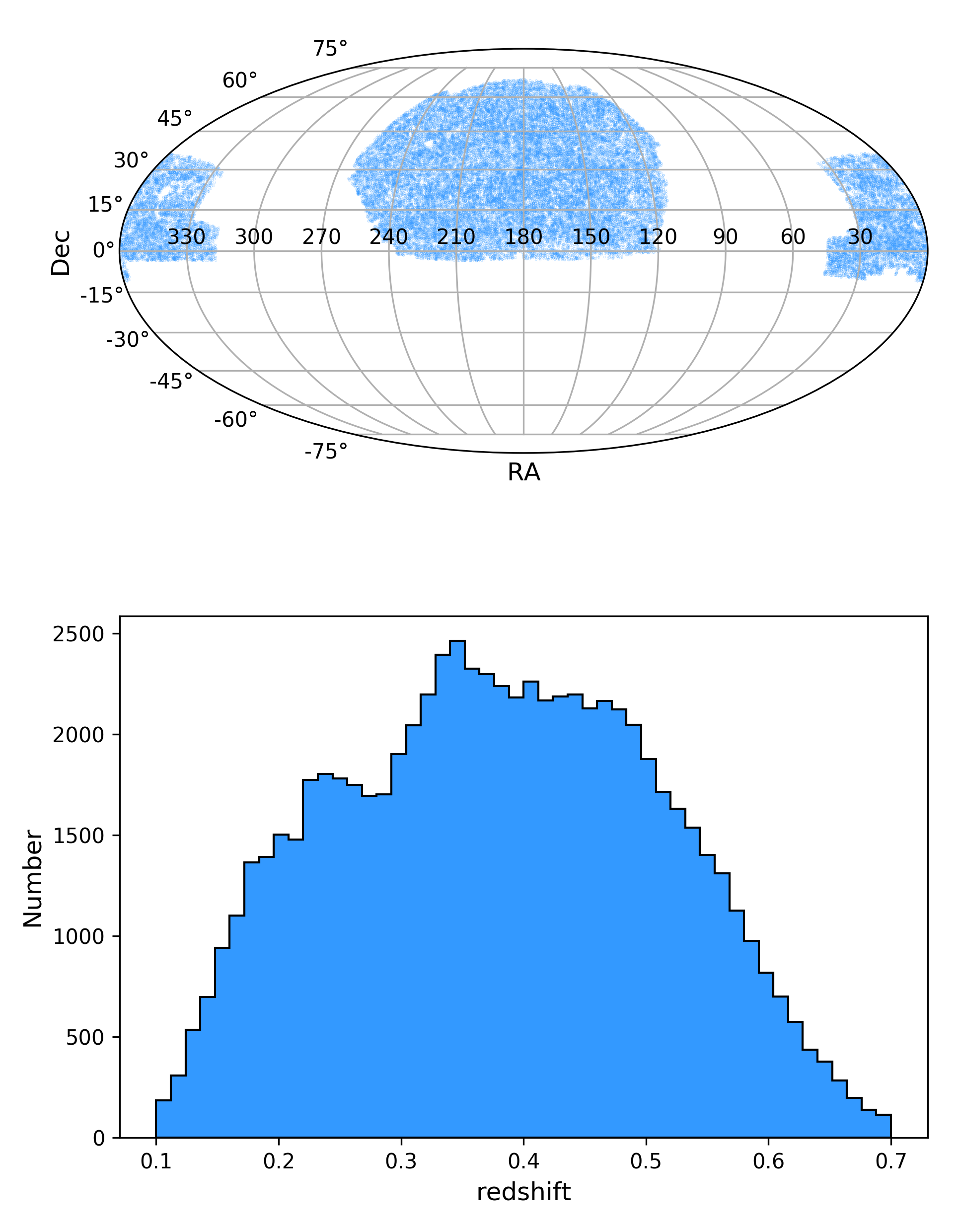
Figure 1: Angular position and redshift distribution of the galaxy cluster sample.

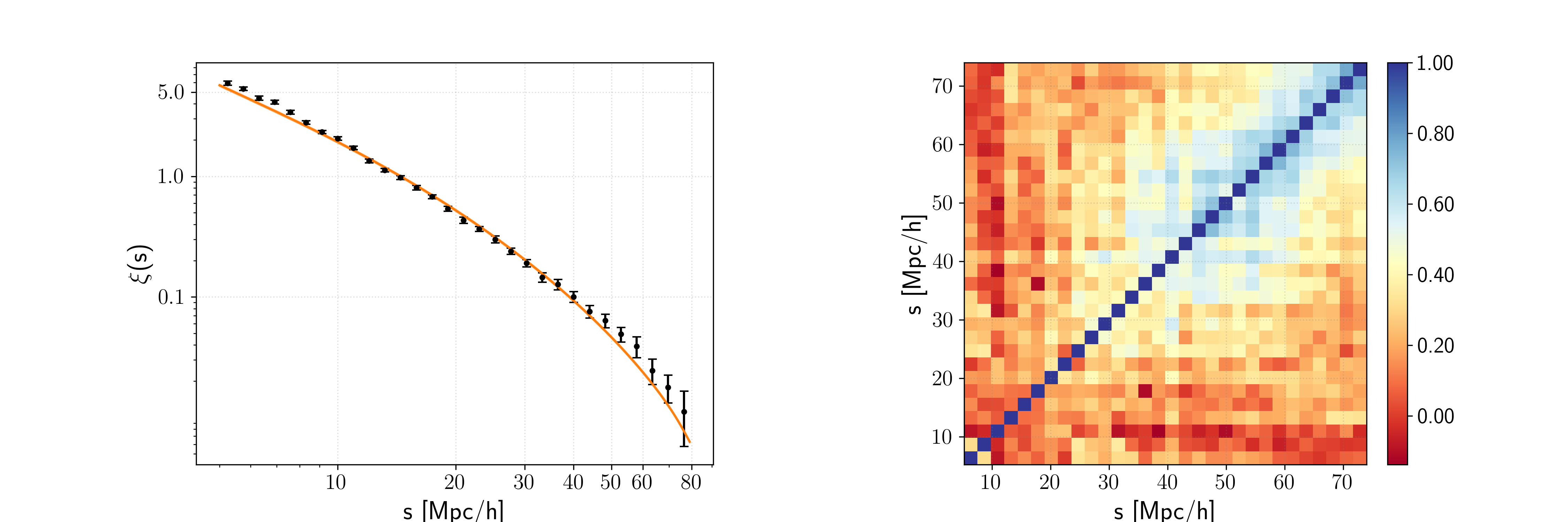
Figure 2: Monopole of the 2PCF. Left panel: the measurements compared to the best-fit model (orange line and shaded area indicating the 68% confidence level). Right panel: the corresponding correlation matrix.

4 Analysis

In this Section, we present the analysis performed to measure the 3PCF of galaxy clusters, the constraints obtained on the bias parameters, and a comparison with results obtained in the literature.

4.1 The measurements

For the purpose of our analysis, we measure the 3PCF at several different scales, and in different configurations.

As a first step, we assess the bias of the population, thus estimating the 3PCF at intermediate scales. We do not consider the small scales ($r<$10 $h^{-1}$ Mpc) that are not accurately reproduced by models due to the non-linear dynamics. In this first analysis, we do not consider the BAO scales as well, so that our results will not be affected by the BAO model considered. We choose three different configurations, with $r_{12}=10$ $h^{-1}$ Mpc and $r_{13}=$ 30, 50, and 70 $h^{-1}$ Mpc, respectively. For each case, we consider 15 angular bins in $\theta$, defining a third side of the triangle spanning $20<r_{23}<40$ $h^{-1}$ Mpc, $40<r_{23}<60$ $h^{-1}$ Mpc, and $60<r_{23}<80$ $h^{-1}$ Mpc, respectively. In this way, we consider three configurations with a non-overlapping third side, and adopt a 5% tolerance on the $r_{12}$ and $r_{13}$ sides of the triangle, namely $\Delta r_{ij}/r_{ij}=0.05$. With these settings, we measure both the connected, $\zeta$, and the reduced, $Q$, 3PCFs. We explored also other different configurations (not shown here), finding that the main results of the analysis do not change appreciably.

Then to detect the BAO peak, we focus on three different configurations where the BAO peak is included in the third triangle side $r_{23}$, namely $(r_{12},r_{13})=$ (20, 105), (40, 100), and (50, 90) $h^{-1}$ Mpc. The reason behind the choice of these configurations is that they are representative of different regimes at which we expect the BAO signal to be statistically significant, as will be discussed in Sect. 5. Also in this case, we measure both $\zeta$ and $Q$.

The error covariance matrices have been estimated with a JK approach, considering 100 sub-volumes. We verified that changing this value to a higher sampling has a negligible impact on the resulting errors. Therefore, in the following analysis, we will adopt this choice which allows us a fast enough numerical computation.

Finally, we also measure the monopole of the 2PCF on the same catalog. We use the Landy & Szalay (1993) given by Eq. (3), with 30 logarithmically-spaced bins in the range $5<r$[$h^{-1}$ Mpc]$<80$. These data will be helpful to provide further additional information on the bias of our sample in our analysis, as discussed in Sect. 4.2.

The measurements for the 2PCF and the 3PCF are presented in Figs. 2 and 3. All of them have been performed assuming a Planck18 cosmology to convert observed coordinates into comoving ones. We also tested the results assuming a Planck15 (Planck Collaboration et al., 2016) cosmology, finding differences smaller than 1-$\sigma$.

4.2 Estimating the bias

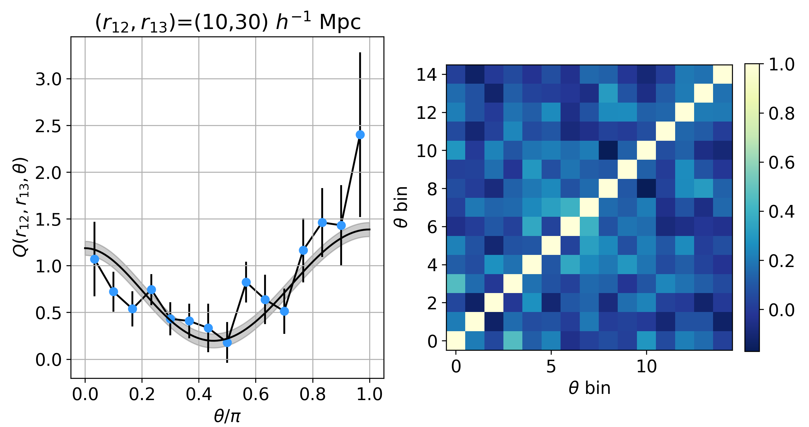
Figure 3: 3PCF measurements for SDSS galaxy clusters at intermediate scales. The considered configurations have been chosen to have the first side $r_{12}=10$ $h^{-1}$ Mpc and the second side $r_{13}=$ 30, 50, and 70 $h^{-1}$ Mpc, from top to bottom. As a result, the third side spans the ranges $20<r_{23}$[$h^{-1}$ Mpc]$<40$, $40<r_{23}$[$h^{-1}$ Mpc]$<60$, and $60<r_{23}$[$h^{-1}$ Mpc]$<80$, respectively. The left panels show the reduced 3PCF $Q$, while the right ones the corresponding correlation matrices. The best-fit 3PCF models are shown as a black curve in the left panels, with their associated 1-$\sigma$ uncertainties as shaded grey area.

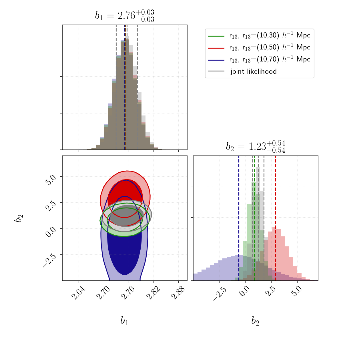
Figure 4: Constraints on $b_{1}$ and $b_{2}$ from the configurations shown in Fig. 3 (shown in different colors) and from the joint analysis of all scales (in gray).

To constrain the bias parameters of the selected galaxy cluster sample, we fit the reduced 3PCF, $Q(\theta)$, which provides the advantages discussed in Sect. 2.2, that is to break the degeneracy between bias parameters and $\sigma_{8}$ (see e.g. Kayo et al., 2004; Zheng, 2004; Guo & Jing, 2009; Marín, 2011; McBride et al., 2011; Guo et al., 2014, 2016).

As presented above, different models can be explored to fit the 3PCF, including bias parameters at different levels. We investigated the possibility of fitting our data with both Eqs. (6) and (7). Due to the statistics of the current sample, we verified that the SNR is too low for a 3-parameters fit. Therefore we excluded the possibility of constraining the tidal parameter $g_{2}$, and in the following analysis we will consider only the model provided by Eq. (6).

Unfortunately, the degeneracy between $b_{1}$ and $b_{2}$ in the fit of the reduced 3PCF does not allow us to obtain constraints enough stringent, even with two parameters only. We, therefore, decided to include in the analysis the additional information coming from the 2PCF, to constrain the bias parameter $b_{1}$. Specifically, we model the monopole of the 2PCF in redshift space, $\xi(s)$, as follows (Kaiser, 1987; Hamilton, 1992):

$$\xi(s)=\left[(b_{1}\sigma_{8})^{2}+\frac{2}{3}f\sigma_{8}\cdot b_{1}\sigma_{8}+\frac{1}{5}(f\sigma_{8})^{2}\right]\frac{\xi_{\rm DM}(r)}{\sigma_{8}^{2}}\;,$$ (8)

where $f\simeq\Omega_{\rm M}^{0.545}(z)$ is the linear growth rate of cosmic structures, and $\xi_{\rm DM}(r,z)$ is the real-space dark matter 2PCF estimated by Fourier transforming the linear matter power spectrum, computed with CAMB (Lewis & Bridle, 2002). We fit the 2PCF in the range $10<s$[$h^{-1}$ Mpc]$<60$, considering its associated covariance matrix, and assuming a flat prior on $b_{1}$ between $0$ and $4$. We limited our analysis in this range because, while the correlation matrix is almost diagonal below 60 $h^{-1}$ Mpc, it presents a significant correlation between different bins above, as can be seen in Fig. 2. However, we checked that changing $s_{min}$ down to 5 $h^{-1}$ Mpc and $s_{max}$ up to 80 $h^{-1}$ Mpc, the obtained constraints on the bias show a negligible variation, below the 1% level. From the fit of the 2PCF monopole, we obtain $b_{1}=2.75\pm 0.03$. Veropalumbo et al. (2016) measured and modeled the 2PCF of this same sample, but splitting it into three subsamples depending on the survey they were belonging to (SDSS-MGS, BOSS-LOWZ, and BOSS-CMASS). We find that our result is fully compatible with theirs once averaged, with a difference smaller than 1-$\sigma$ (taking into account the different cosmological model assumed). In this analysis, we decided not to divide our sample into smaller sub-samples since we verified that it would lower the statistics, increasing the shot-noise excessively.

We use this bias measurement as a Gaussian prior in our 3PCF analysis, when exploiting the model given by Eq. (6) to place constraints on the non-linear bias parameter, $b_{2}$, for which we assume a flat prior in the range $-20\leq b_{2}\leq 20$.

Table 1: Bias parameter estimates for the SDSS galaxy cluster catalog. The linear bias is estimated from the 2PCF (assuming Planck18 cosmology), while the non-linear bias from the 3PCF (assuming Planck18 cosmology and a Gaussian prior on $b_{1}$ from the 2PCF). The constraints for the non-linear bias are shown at different scales. The last line shows the result from the combined fit at all scales.

method	scales [$h^{-1}$ Mpc]	$\rm b_{1}$	$\rm b_{2}$	$\chi^{2}$/d.o.f
2PCF	$10<s<60$	$2.75\pm 0.03$	–	1.3
3PCF	$20<r_{23}<40$	–	$0.9\pm 0.6$	1.1
3PCF	$40<r_{23}<60$	–	$2.9\pm 1.2$	1.2
3PCF	$60<r_{23}<80$	–	$-0.6\pm 2.6$	0.7
3PCF	joint scales	–	$1.2\pm 0.5$

We fit $Q(r_{12},r_{13},\theta)$ at the different scales presented in Sect. 4.1, considering the associated covariances. The results are shown in Figs. 3 and 4, and summarized in Tab.1. We find an increasing precision on the $b_{2}$ constraint with decreasing scale, that can be expected as the errors on $Q$ are smaller at smaller scales, due to the higher number of triplets that can be found in these configurations. In all cases, the best-fit model well reproduces the data, except in the intermediate bin, with ($r_{12},r_{13})$=(10,50) $h^{-1}$ Mpc, where a larger discrepancy is observed. This effect is due to the fact that the prior on $b_{1}$ fixes the shape of the model, while the parameter $b_{2}$ (left free in the fit) controls its normalization (see Eq. 6). In all cases, however, the reduced $\chi^{2}$ is between 0.7 and 1.2. Given that we chose non-overlapping configurations in $r_{23}$, we also performed a joint fit to the three scales. The results are presented in Fig. 4, showing the 68% and 95% confidence contours for $b_{1}-b_{2}$, and their marginalized distribution. The combined analysis has been performed using the emcee software (Foreman-Mackey et al., 2013), which is a Python code that provides a Markov Chain Monte Carlo (MCMC) implementation of the affine-invariant ensemble sampler of Goodman & Weare (2010). The final value we obtain from the analysis of the combined scale is $b_{2}=1.2\pm 0.5$.

4.3 The advantage of cluster as tracers

We compare our results both with independent estimates and with theoretical forecasts. Lazeyras et al. (2016) provided a theoretical relation between the expected values of $b_{1}$ and $b_{2}$ from N-body simulations. Using the constraints on $b_{1}$ we obtained from the analysis of the 2PCF and their Eq. 5.2, we obtain $b_{2}=1.70\pm 0.08$, consistent with our measurement. Comparing our constraints with other analyses of real galaxy catalogs in the same redshift range, we find instead some differences, which are, however, mostly ascribable to a difference in the tracers analyzed. Slepian et al. (2017a), from the analysis of the 3PCF of SDSS-DR12 CMASS galaxies, found $b_{2}(z=0.565)=0.3\pm 0.7$; Marín et al. (2013) measured the 3PCF of the WiggleZ Dark Energy Survey in three redshift bins, finding $b_{2}(z=0.35)=-0.36^{+0.11}_{-0.08}$, $b_{2}(z=0.55)=-0.41^{+0.09}_{-0.08}$, and $b_{2}(z=0.68)=-0.48^{+0.14}_{-0.12}$. These discrepancies in the non-linear bias can be explained by taking into account that in Slepian et al. (2017a) the sample consisted in very massive galaxies (log$(M/M_{\odot}\sim$11.3) at $z\sim 0.5$ (Maraston et al., 2013) but still less biased than our tracers, while the WiggleZ survey was mostly focused in selecting star-forming galaxies at $z\sim 0.5$ (Marín et al., 2013). The linear bias is $b_{1}=2.23\pm 0.06$, $0.72\pm 0.14$, $0.99^{+0.10}_{-0.09}$, and $1.06^{+0.16}_{-0.18}$, respectively, significantly lower than the one of our clusters. If we consider the previously discussed $b_{2}(b_{1})$ relation, we find that this difference in linear bias compensates for the differences in the non-linear bias results.

It is interesting to notice that while this analysis, given the current number of galaxy clusters available, is shot-noise dominated, it already shows clearly the advantage of a galaxy cluster sample with respect to a sample with a smaller bias. On one side, selecting objects in the peak of matter over-densities significantly reduces the effects due to non-linear dynamics, as also found by Marulli et al. (2020). On the other side, to assess more quantitatively the improvement of using such a sample we also perform a complementary analysis. We use the publicly available SDSS-BOSS galaxy and random catalogs, and extract from these a sample with the exact same statistics and redshift distribution of our cluster sample. In this way, the only differences that we will find in the results can be attributed to the different tracers. We analyze this catalog with the same method described in Sect. 4.1, and as a first result we confirm that this sample is characterized by a smaller bias, $b_{1}=1.95\pm 0.02$. We then compare the percentage errors associated to the measured reduced 3PCF, and find that the cluster catalog has an error on average $\sim$20% smaller than the galaxy catalog. This results in a constraint on $b_{2}$ from the fit of the reduced 3PCF with errors $\sim$20% smaller. This highlights the gain in using more biased tracers in the analysis.

5 Detecting the BAO peak in the 3PCF of galaxy clusters

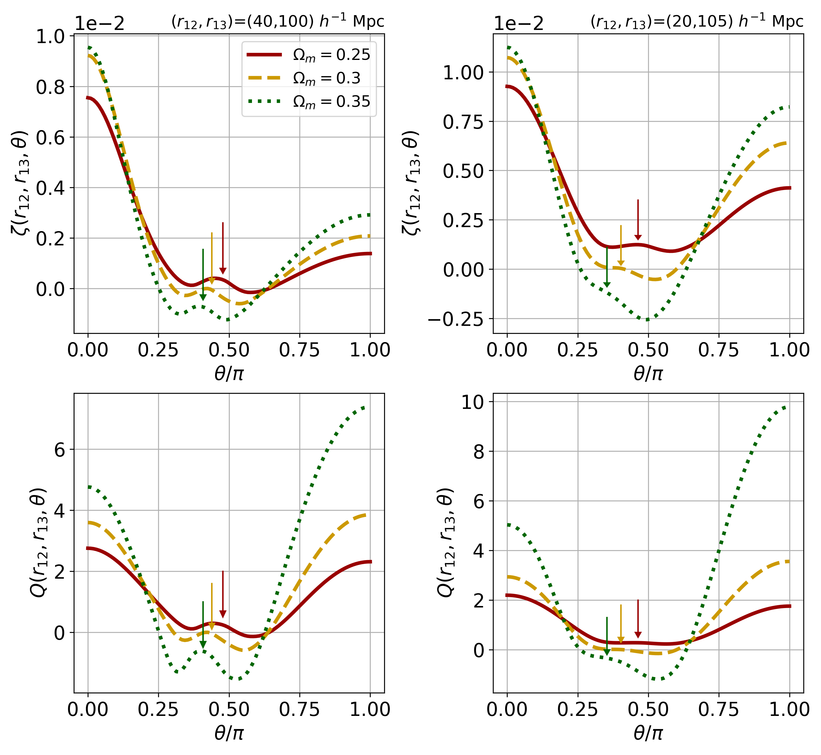
Figure 5: Examples of the BAO detectability in the 3PCF as a function of $\Omega_{m}$ (represented by different line colors, as shown in the legend) for the connected 3PCF (upper panels) and for the reduced 3PCF (lower panels). Different scale configurations are shown, $(r_{12},r_{13})=$ (40,100) $h^{-1}$ Mpc (left panels) and (20,105) $h^{-1}$ Mpc (right panels). In each panel, a colored arrow show the position of the BAO peak for each model.

The BAO feature appears as a clear peak around 100 $h^{-1}$ Mpc in the 2PCF. The peculiar shape of the 3PCF, however, makes a bit more difficult to clearly detect this peak, since both $\zeta(\theta)$ and $Q(\theta)$ are characterized by a U- or V-shape, with a sharp dip around $\theta\sim\pi/2$ (see, e.g., Fig. 3). Therefore, when probing BAO scales, the shape of the 3PCF will show a complex behavior, with different features depending on the relative depth and height of the dip and peak.

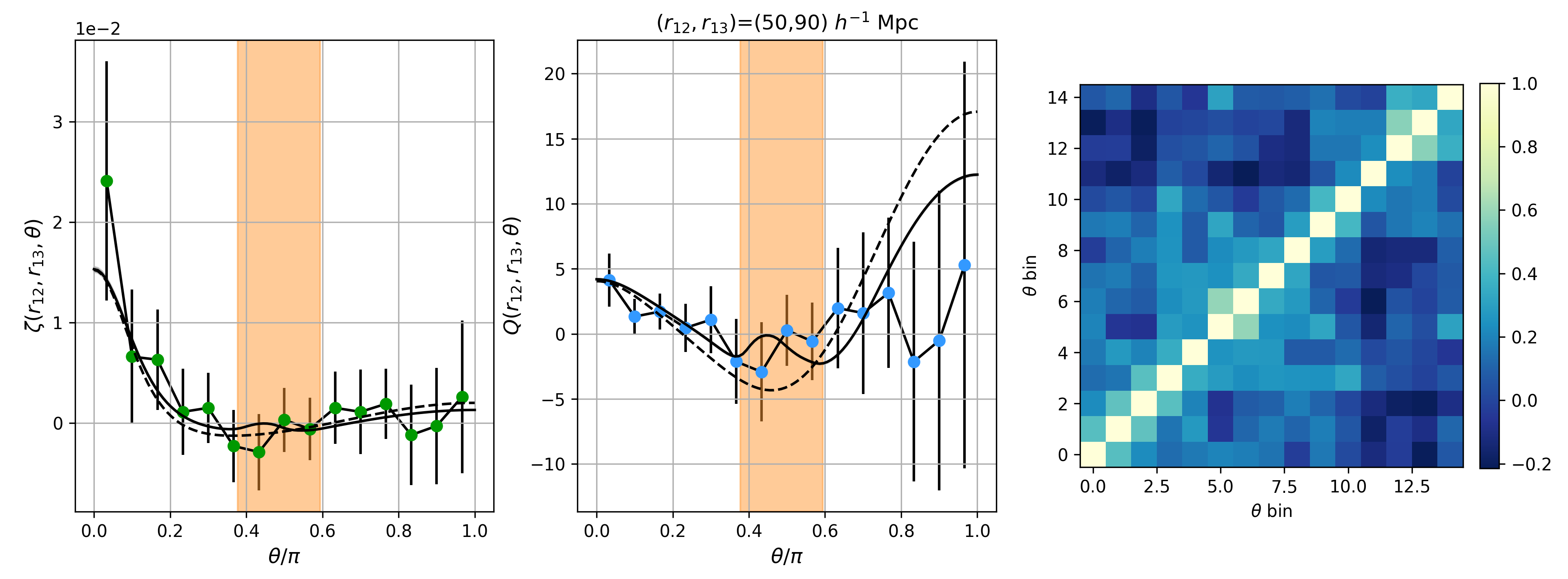
Figure 6: 3PCF measurements for SDSS galaxy clusters at BAO scales. Left panels: the connected 3PCF; central panels: the reduced 3PCF; right panels: the correlation matrices of the reduced 3PCF. The configurations chosen are, from top to bottom, $(r_{12},r_{13})=$ (20, 105), (40,100), and (50, 90) $h^{-1}$ Mpc, respectively. The orange shaded area shows the region $85\leq r_{23}$[$h^{-1}$ Mpc]$\leq 115$, to highlight the expected position of the BAO peak. The black lines show the model at the best-fit parameters obtained by fitting 3PCF as smaller scales (Sect. 4.2), while the dashed line is a model assuming the same parameters, but without the BAO peak. The BAO peak can be detected in the reduced 3PCF with a clearer evidence from top to bottom panels as the difference between the two models.

In Fig. 5, we show an example of how the results may appear in different configurations, for both the connected and reduced 3PCFs, for different values of $\Omega_{m}$ (keeping fixed all other cosmological parameters, including the power spectrum normalization). We used CBL to produce 3PCF models, focusing in particular on the two configurations$(r_{12},r_{13})=$ (40,100) and (20,105) $h^{-1}$ Mpc, representing two typical behaviors of the 3PCF. We find that, at fixed configuration, the BAO peak is sharper and more detectable in the reduced 3PCF rather than in the connected 3PCF. Cosmological parameters have also an impact on the BAO visibility, with a higher peak corresponding to a higher value of $\Omega_{m}$. As for the dependence on the configuration, we find that the dip of the 3PCF and the BAO peak can combine themselves in two ways: they can be of the same order of magnitude, thus canceling out each other, and giving a flat 3PCF shape for $\theta\sim\pi/2$ (as can be seen e.g. in the case $(r_{12},r_{13})=$ (40,100) $h^{-1}$ Mpc), or the BAO peak can dominate, resulting in a small peak embedded in the dip (as e.g. for the case $(r_{12},r_{13})=$ (20,105) $h^{-1}$ Mpc). This effect is due to the fact that it is possible to choose configurations that concentrate the BAO signal on a smaller or on a wider $\theta$ range: in the case of $(r_{12},r_{13})=$ (20,105) $h^{-1}$ Mpc, the third side, $r_{23}$, ranges between 85 and 125 $h^{-1}$ Mpc, and the BAO peak is spread approximately on the entire $\theta$ range, while for $(r_{12},r_{13})=$ (40,100) $h^{-1}$ Mpc the BAO signal is concentrated in $0.3\leq\theta\leq 0.5$, with higher visibility.

For the above reasons, we decided to focus on the three configurations discussed in Sect. 4.1, in order to exploit different possibilities to detect the BAO peak. The results are shown in Fig. 6 for configurations progressively concentrating the BAO signal on a smaller range of angles. First, we recover that the less concentrated the BAO peak is, the flatter the resulting 3PCF spread over a smaller number of bins is that the final signal-to-noise ratio of the measurement is smaller, and the evidence of a peak less clear. We compare the measurements of the 3PCF with theoretical models assuming the best-fit parameters estimated in the previous analysis of Sect. 4.2 (solid lines). Here, we remind that we decided to fit $Q(\theta)$ rather than $\zeta(\theta)$, therefore some discrepancies between models and data in the connected 3PCF are expected. We find that the obtained models well reproduce the measured reduced 3PCF, with a reduced $\chi^{2}$ between 0.3 and 0.7; the small values of the reduced $\chi^{2}$ are caused by the large errors associated to the 3PCF especially at the largest angles, due to the smaller number of triplets at the largest probed scales.

Figure 6 presents also the models obtained with the same parameters, but from a no wiggle power spectrum that does not include the BAO peak obtained with the CBL from the prescriptions of Eisenstein & Hu (1998). We notice that while in the connected 3PCF the differences between the two models are only at BAO scales, as expected, in the reduced 3PCF a significant deviation appears also for $\theta>0.7$. This effect is due to the fact that $Q(\theta)$ is defined as the connected 3PCF normalized by a combination of $\xi^{2}(r)$ (see Eq. (4)). At the large scales where this deviation is detected ($r>110$ $h^{-1}$ Mpc), the 2PCF becomes smaller and smaller (see Fig. 2), and eventually close to zero due to random fluctuations caused by Poisson noise. This produces the large variations that are observed in $Q(\theta)$, but not in $\zeta(\theta)$.

To quantify the detectability of the BAO peak, we use the same approach adopted in Slepian et al. (2017a), estimating the difference in $\chi^{2}$ between the best-fit models including or not the BAO, $\rm\Delta\chi^{2}_{noBAO-BAO}$. To avoid being biased by the previously discussed fluctuations in the 2PCF, we restrict our $\chi^{2}$ estimate to the angles corresponding to $85\leq r$[$h^{-1}$ Mpc]$\leq 105$ (as also highlighted by the orange shaded area in Fig. 6), that is close to the position of the BAO peak. The results are reported in Tab. 2.

We find that for all the configurations probed, the model including the BAO reproduces the observed reduced 3PCF better than the one without the BAO, with a difference $\rm\Delta\chi^{2}_{noBAO-BAO}$ between $\sim$2 and $\sim$75. The configuration that shows the largest evidence for the presence of the BAO peak is $(r_{12},r_{13})$ = (25,105) $h^{-1}$ Mpc, where the BAO signal is spread over a larger number of bins. In the other configurations, the BAO feature is squeezed in a smaller number of bins and, as expected from previous considerations, it shows some hints of a peak both in the connected and in the reduced 3PCF. These configurations, however, also show a larger error, and therefore the resulting evidence is lower, but still preferring the presence of a BAO peak.

These data represent the first detection of the BAO signal in the 3PCF of galaxy clusters. Moreover, they also pave the way to select the best configurations to detect the BAO signal in the 3PCF, showing that it has a stronger signal in the reduced than in the connected 3PCF, and that the configurations maximizing the signals are the ones for which the BAO peak is sampled on a larger number of bins. To further systematize these results, in the next section we will discuss a theoretical framework to estimate the SNR of the BAO peak in the 3PCF as a function of the configuration probed.

Table 2: Differences in $\chi^{2}$ between models with and without BAO (assuming Planck18 cosmology). The $\Delta\chi^{2}$ have been estimated in the range of separations interested by the BAO feature, corresponding to the orange band in Fig. 6.

scales	$\rm\Delta\chi^{2}_{noBAO-BAO}$
$r_{12}=25$ $h^{-1}$ Mpc, $r_{13}=105$ $h^{-1}$ Mpc	74.9
$r_{12}=40$ $h^{-1}$ Mpc, $r_{13}=100$ $h^{-1}$ Mpc	21.6
$r_{12}=50$ $h^{-1}$ Mpc, $r_{13}=90$ $h^{-1}$ Mpc	2.1

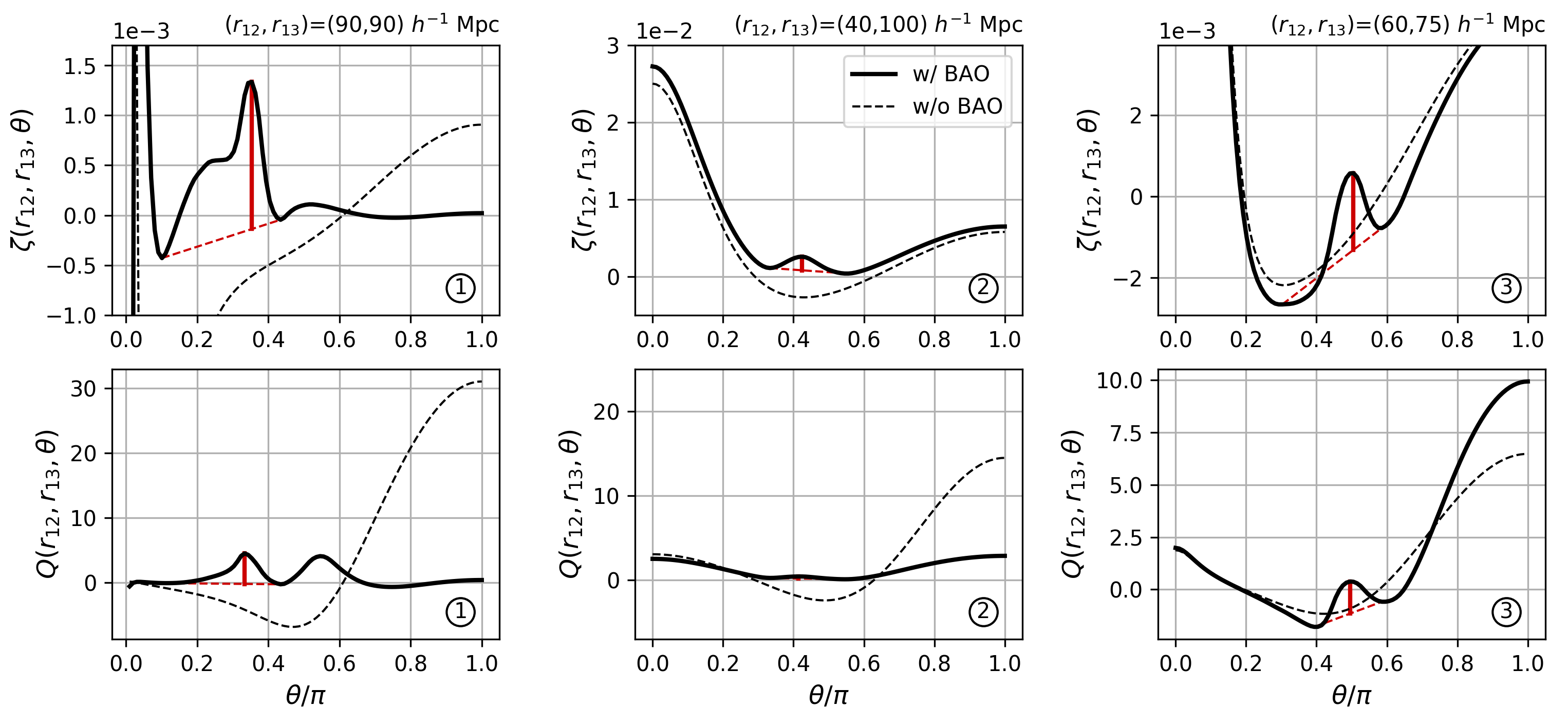
Figure 7: Examples of theoretical 3PCF estimates. The top panels show the connected 3PCF at three scales, namely $(r_{12},r_{13})$=(90,90), (40,100), and (60,75) $h^{-1}$ Mpc (panels from left to right), while the lower panels show the associated reduced 3PCFs. In all panels, black solid lines show the model including the BAO, while the dashed lines the model without the BAO. The red lines show the estimated BAO contrast, as discussed in Sect. 6.1. Each panel is also labelled with a number, showing the position of the configuration in the following Figs. 8 and 9.

6 BAO detectability in the 3PCF of Euclid clusters

As previously discussed, one of the main results of this work is that the BAO peak in the 3PCF can be more or less evident depending on the considered configuration. For this reason, in Sect. 4 we analyzed three different configurations of scales. In this Section, we provide a framework in order to forecast which are the most favorable configurations to detect the BAO peak in the 3PCF, both for the connected and the reduced 3PCFs, and apply it to the case of the Euclid mission as an example of a future wide survey of galaxy clusters.

For this purpose, we need three ingredients: (i) a theoretical estimate of the BAO signal in the 3PCF at various scales, (ii) a theoretical estimate of the expected corresponding error, and (iii) an estimate of the associated SNR.

6.1 The BAO signal in the 3PCF

As a first step, we used the CBL to compute theoretical 3PCF models following Barriga & Gaztañaga (2002). To provide forecasts on the detectability of the BAO peak with Euclid clusters, we base our analysis on the expected number density and mass for these objects estimated in the work of Sartoris et al. (2016). We assume a Euclid-like survey that will detect approximatively 2$\times 10^{5}$ clusters with S/N>3 in the Euclid photometric survey (Laureijs et al., 2011) in the range $0.2<z<2$, with masses log$(M/M_{\odot}\gtrsim$13.9 and a mean redshift $<z>\sim 1$; the effective bias $b_{1}$ has been estimated from the scale relation by Tinker et al. (2010) ($b_{1}=5.4$), and the non-linear bias parameter $b_{2}$ from the relation by Lazeyras et al. (2016) ($b_{2}=17.4$), assuming a Planck18 cosmology.

The models have been created considering every possible closed triangle configurations with $r_{12}$ and $r_{13}$ between 30 and 115 $h^{-1}$ Mpc, with a binning of 5 $h^{-1}$ Mpc. The third side $r_{23}$ spans all the possible allowed values between $r_{min}=r_{13}-r_{12}$ and $r_{max}=r_{13}+r_{12}$; therefore, by definition for some combinations the BAO peak will not be visible in $\zeta(\theta)$ and $Q(\theta)$, but in the majority it will.

To measure the BAO signal in the 3PCF, two approaches have been considered.

• BAO from model comparison. The first approach, similar to the one considered in Sect. 5, is to measure the difference between 3PCF models with and without the inclusion of the BAO signal. In this case, we average the values of the 3PCF in the range of $\theta$ such as $85<r_{23}$[$h^{-1}$ Mpc]$<115$, i.e. the scales for which the BAO peak is observed at these redshifts, for both models, and estimate the difference between these two values. We define this value as BAO difference. This has been done for both the connected and the reduced 3PCFs.

• BAO contrast. In the second approach, to be less model dependent, we only consider the model including BAO, and measure if it is possible to detect the presence of a peak in the 3PCF. As previously discussed, this is not a trivial task, since given the shape of the 3PCF it means to detect a secondary peak between two larger peaks in the 3PCF that usually are at $\theta\sim 0$ and $\theta\sim\pi$. To do this, we use the modules argrelmin and argrelmax of the scipy.signal Python library (Virtanen et al., 2020), specifically designed to detect relative maxima and minima in a function. To define a peak, and, most importantly, its height, we therefore use these functions to detect a relative maximum between $0<\theta<\pi$, and its adjacent relative minima. These relative minima are used to define a baseline for the peak by linearly interpolating between them, and the height of the peak is then measured as the distance between the relative maximum and the baseline. We define this value as the BAO contrast. As for the previous approach, this has been estimated both on $\zeta(\theta)$ and $Q(\theta)$.

For illustrative purposes, in Fig. 7 we show some examples of the generated 3PCFs, including both the models with and without the BAO signal, and a visual representation of the BAO contrast.

6.2 A theoretical estimate of the 3PCF covariance

To estimate the errors, we consider the theoretical covariance as defined by Slepian & Eisenstein (2015) (see their Sect. 6.2, and Eq. 51), and included in the CBL. This formula provides an analytical estimate of the covariance depending on two main parameters: the number of objects and the volume of the survey. We consider the volume that will be covered by the Euclid mission with its 15,000 square degrees between $0.2<z<2$, and 2$\times 10^{5}$ clusters as obtained from the forecasts of Sartoris et al. (2016).

The covariance matrices have been calculated for all the simulated configurations (as discussed in Sect. 6.1), and they have been used to estimate the expected errors at the BAO scale, by averaging the errors in the same range used to estimate the BAO signal.

Finally, we estimate the SNR of the BAO signal by dividing the estimated value, either the BAO difference or the BAO contrast, and the estimated error. In this way, we obtain the six maps that are shown in Figs. 8 and 9, one for the signal, one for the error and one for the SNR, for both the connected and the reduced 3PCFs. These maps can be used to forecast which are the preferable configurations that maximize the BAO peak in the 3PCF.

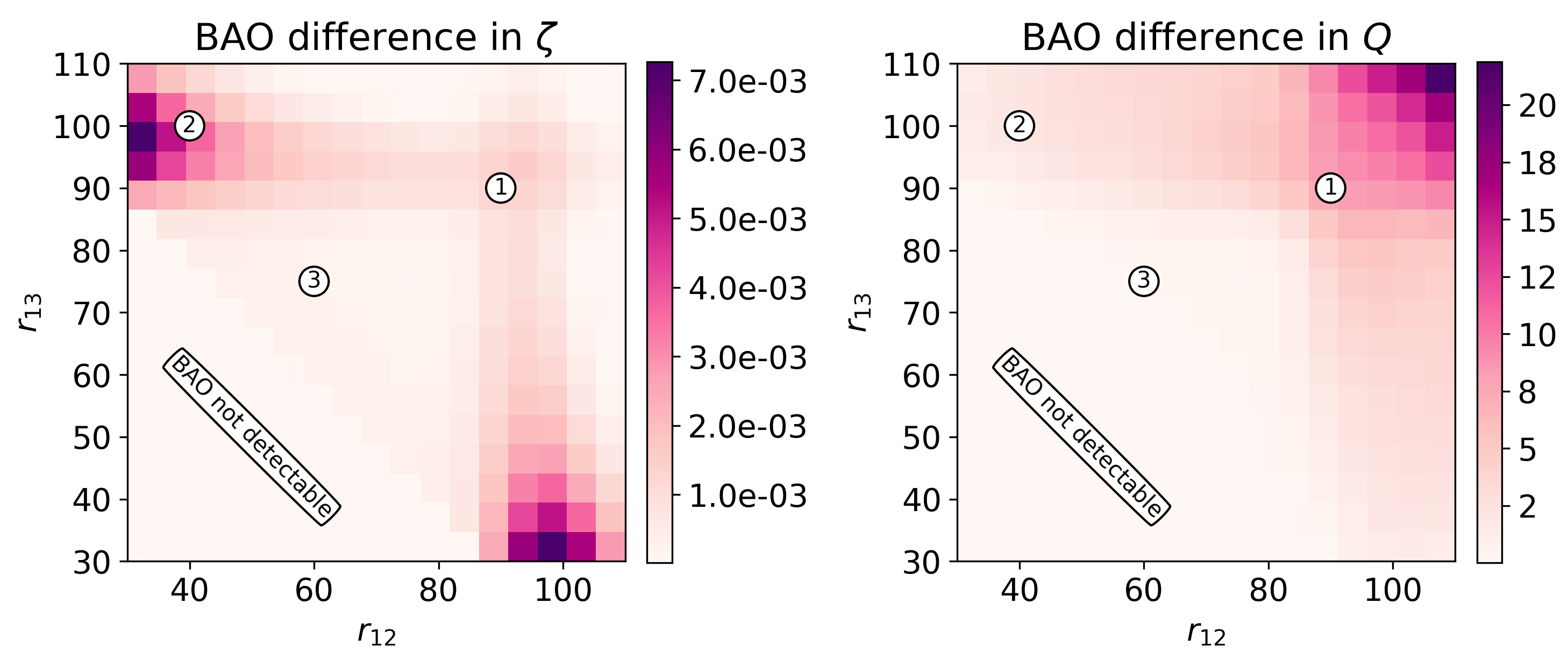
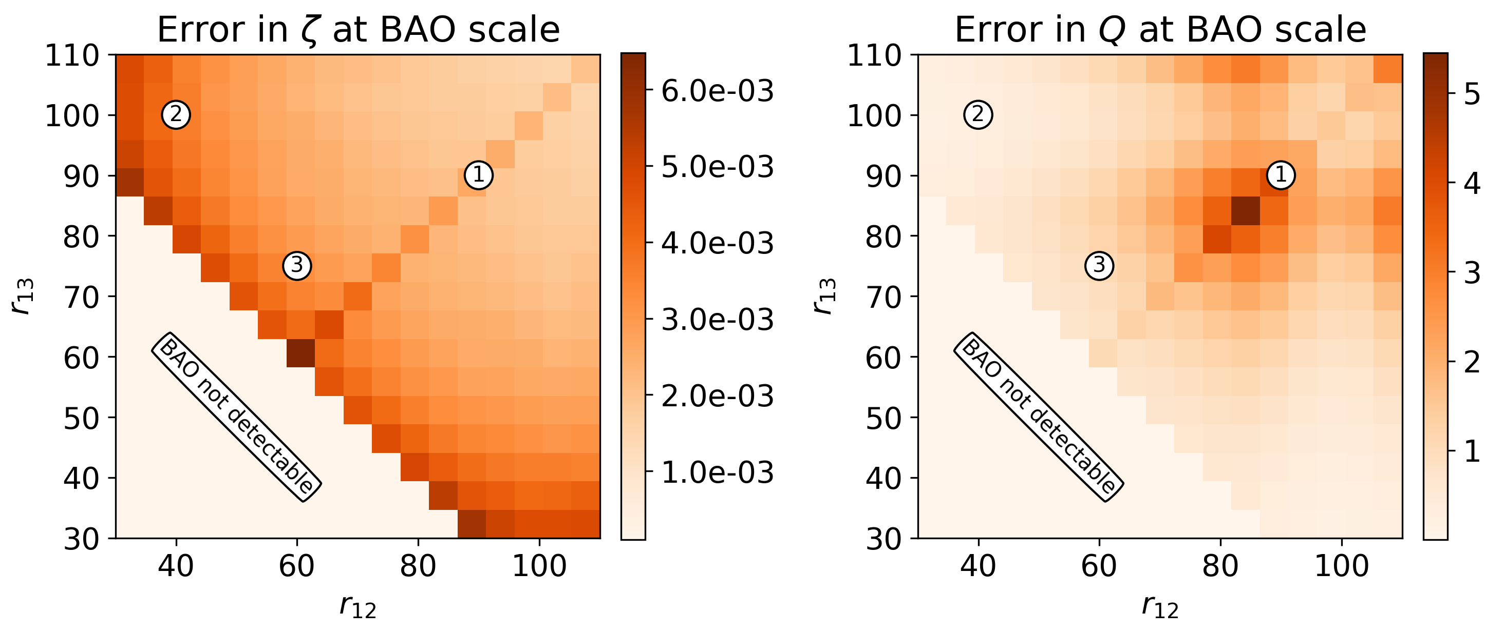
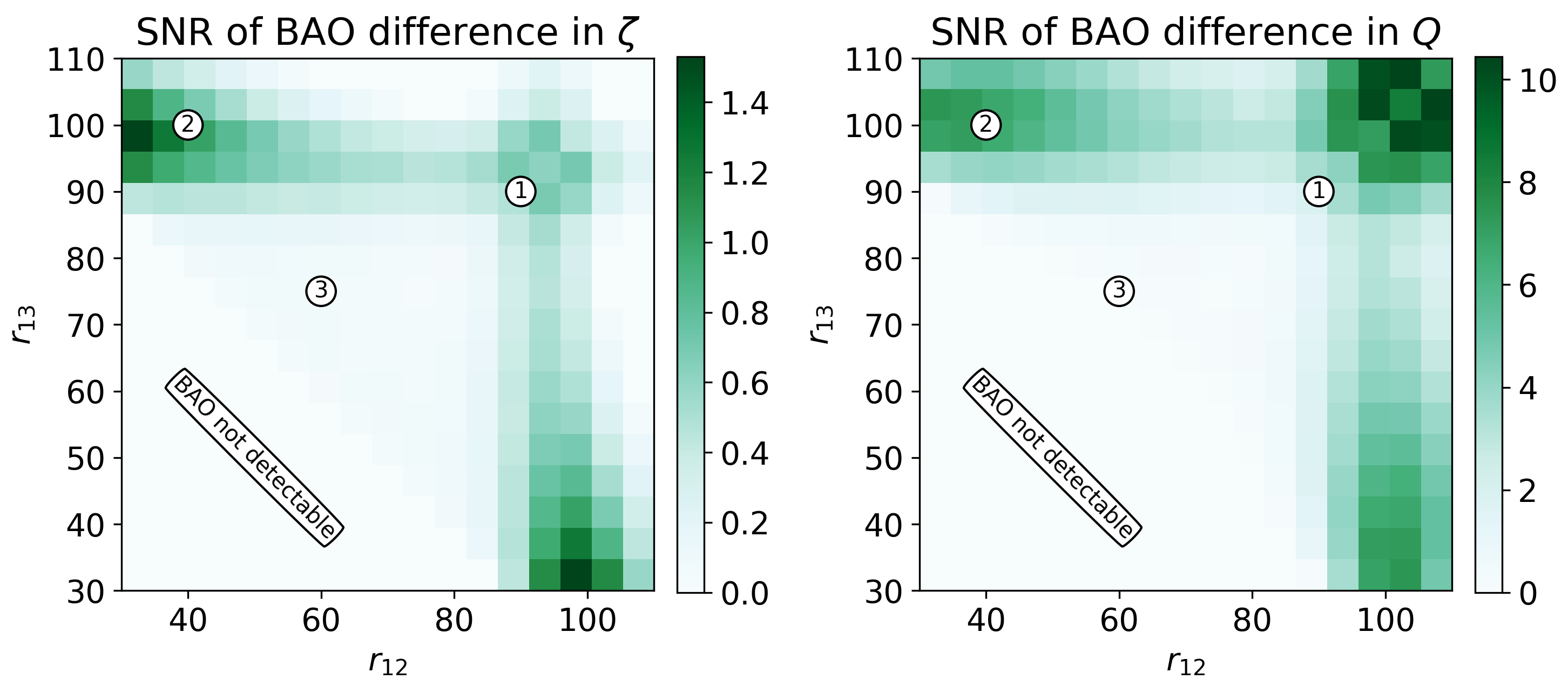
Figure 8: BAO detectability in the 3PCF for the BAO difference case for both the connected and reduced 3PCFs (left and right panels, respectively). From top to bottom, the different panels show: the detectability BAO signature, estimated as the difference between models with and without BAO; the expected errors (as described in Sect. 6.2); the SNR of the BAO peak. The region where the BAO peak is not visible is shown in the bottom-left part of each panel. We indicate with labels the position of the configurations shown in Fig. 7.

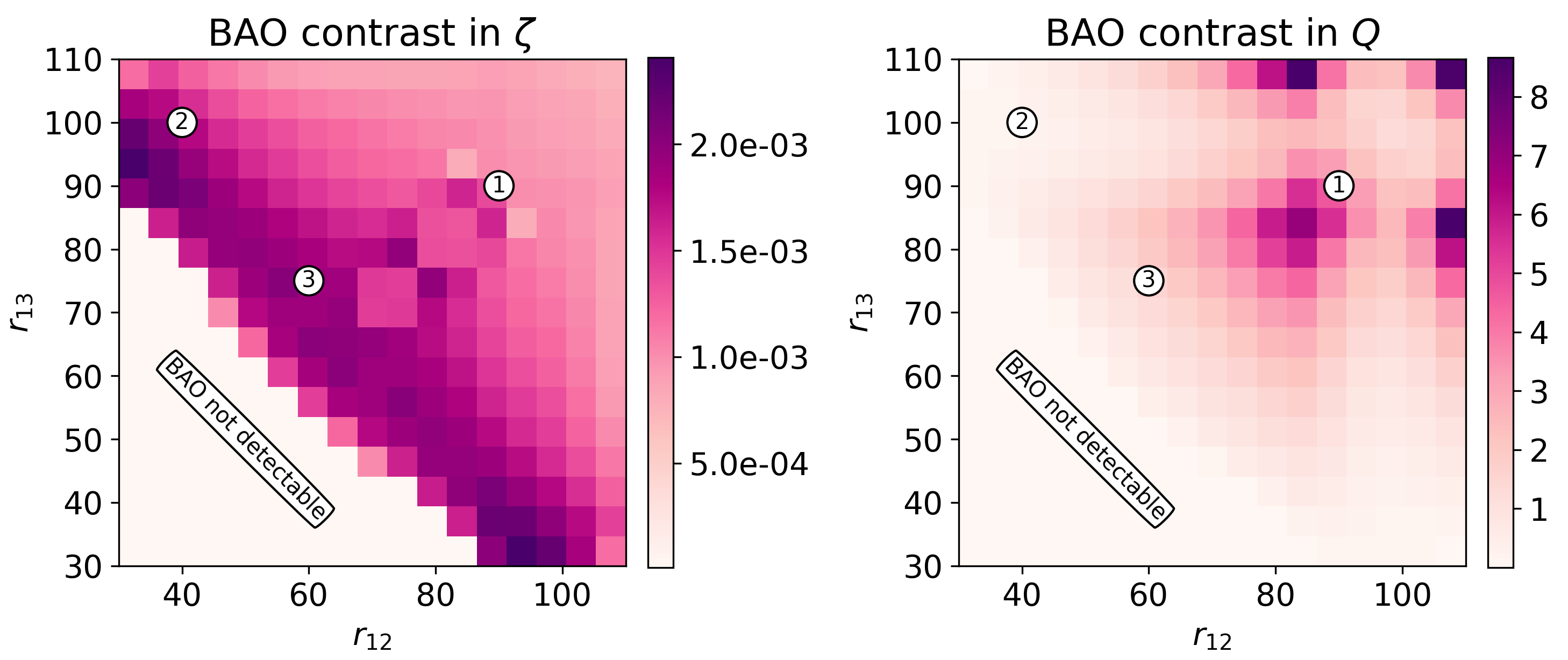
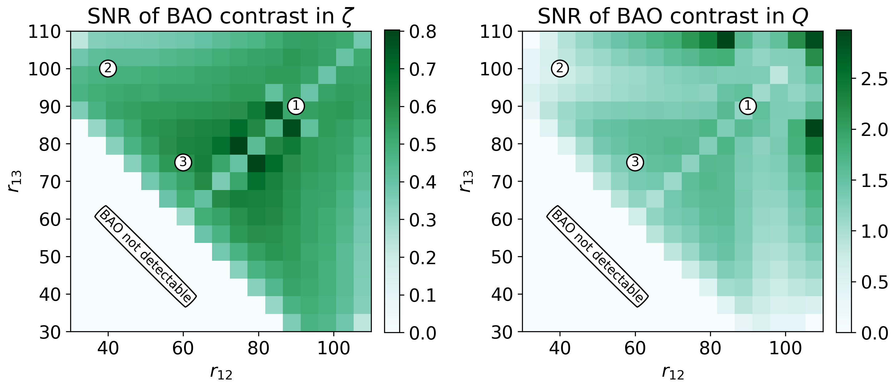
Figure 9: Same as Fig. 8, but showing the detectability of the BAO peak as its contrast with respect to the overall shape of the 3PCF. This measurement would allow a determination of BAO position.

6.3 Discussion

Figure 8 reports the results for the BAO difference case. As can be seen, even for the signal itself, the result is quite different in the connected and reduced 3PCF cases, the former one being maximal for configurations close to $(r_{12},r_{13})$=(40,100) $h^{-1}$ Mpc, while the second one being higher for the equilateral configuration where all three sides are closer to the BAO scale. The errors, however, follow a different distribution, being larger for isosceles configurations with a smaller size in $\zeta(\theta)$, while presenting a peak around $(r_{12},r_{13})$=(80,80) in $Q(\theta)$. As a result, the distribution of the expected SNR is very different between the connected and reduced 3PCF. In the first case, we find that it is maximum for configurations close to $(r_{12},r_{13})$=(40,100) or (90,90) $h^{-1}$ Mpc, but with smaller values of the SNR, SNR$\sim 1.5$ at maximum. On the other hand, the results obtained for the reduced 3PCF are more promising, with high SNR for configurations $(r_{12},r_{13})$=(40,100) and (90,90) $h^{-1}$ Mpc, and values of the order of SNR$\sim 6-10$. This reflects also the results found from the analysis of the data shown in Fig. 6, where it is evident that the difference between the models with and without the BAO is very small for $\zeta(\theta)$, but much more significant for $Q(\theta)$. This effect highlights even more the advantage of using the reduced 3PCF.

The results obtained from the analysis of the BAO contrast of Fig. 9 show, on average, a smaller predicted value of the SNR, with values of the order of 0.8-2.5 for $\zeta(\theta)$ and $Q(\theta)$ respectively. This is a direct consequence of the fact that the measured BAO contrast is for all configurations smaller than the BAO difference. It is interesting to notice, however, that the configurations where the SNR is maximized is significantly different in the two approaches. The configurations explored in our analysis (discussed in Sect. 6) have been explicitly chosen to capture this variety. While having a smaller probability of detection, we think that the BAO contrast approach is nevertheless promising being less model-dependent, especially for future surveys with which the expected error will be significantly smaller due to the much larger statistics.

7 Conclusions

In this paper, we explored for the first time the possibility of detecting the BAO signal in the 3PCF of galaxy clusters.

We analyze the catalog of galaxy clusters obtained cross-correlating the photometric cluster catalog by Wen et al. (2012) with the spectroscopic information from SDSS-DR12. In this way, we end up obtaining information on the BCGs of each cluster with an accurate estimate of its redshift, fundamental for clustering studies. The final catalog comprises 72,563 objects in the redshift range $0.1<z<0.7$, with a mean redshift $<z>=0.38$. We measure the 3PCF of this sample to provide constraints on the properties of this sample in terms of bias and of the detectability of the BAO peak signal.

Our main results can be summarized as follows:

• We measured both the connected 3PCF, $\zeta(\theta)$, and the reduced 3PCF, $Q(\theta)$, for a variety of configurations, spanning from intermediate scales ($r_{23}=20$ $h^{-1}$ Mpc) up to very large scales ($r_{23}=80$ $h^{-1}$ Mpc). We also measured for the same sample the monopole of the 2PCF $\xi(s)$ in the range $10<s$[$h^{-1}$ Mpc]$<80$.

• We analyzed the 2PCF to get an estimate of the linear bias of the sample, obtaining $b_{1}=2.75\pm 0.03$.

• We used the reduced 3PCF measurements at intermediate scales to place constraints on the non-linear bias of the galaxy clusters in the sample. We considered a two-parameter model from Eq. (6) including $b_{1}$ and $b_{2}$, since we verified that it was not feasible to set constraints on the additional tidal bias $g_{2}$. From the 3PCF modeling, combined with the information on the linear bias from the 2PCF, we obtained a constraint on the non-linear bias $b_{2}=1.2\pm 0.5$, considering a joint fit to the scales $20<r_{23}$[$h^{-1}$ Mpc]$<80$.

• Considering the obtained best-fit values $b_{1}$ and $b_{2}$, we analyzed the reduced 3PCF at large scales, exploring different configurations for which the BAO peak is present in $Q(\theta)$. We compared theoretical models of the 3PCF including or not the BAO feature, finding a significant detection of the BAO peak, with the models considering BAO always having a better $\chi^{2}$, with a difference $\Delta\chi^{2}$ between 2 and 75, depending on the configuration.

• To demonstrate the advantage of using galaxy clusters as tracers, we used publicly available SDSS-BOSS galaxies and random catalogs to select a catalog with the same properties in terms of numbers ad redshift distribution of the cluster one, and measured the 3PCF on this catalog. We found that on average the percentage errors on $Q$ is 20% smaller for the cluster catalog, having, as a consequence, 20% better constraints on bias parameters. We discussed how this effect is a combination of the higher bias and of the smaller impact of non-linear dynamics on the cluster sample.

• We developed a framework to theoretically calculate the expected SNR of the BAO feature in the 3PCF of a generic population, and applied it to provide a forecast for clusters detected with the future Euclid mission. We introduced two possible parameterizations to define the presence of the BAO peak, based (i) on the comparison between models with and without the BAO, and (ii) on the direct detection of a peak in the 3PCF. We calibrated a theoretical covariance on the expected performance to detect clusters that have been forecasted for the Euclid survey, and estimated the expected SNR for both the connected and the reduced 3PCF for a variety of configurations, to find those maximizing its value.

• From this framework, we find that the expected SNR of the BAO feature is systematically higher in the reduced 3PCF, $Q(\theta)$, than in the connected 3PCF, $\zeta(\theta)$. We also provide the configurations that optimize the detection of the BAO signal for a Euclid-like cluster sample.

This paper, the second of the $C^{3}$ project, demonstrates that galaxy clusters are very interesting tracers to be analyzed also with higher- order correlation functions, providing the first significant detection of the BAO peak in the 3PCF of galaxy clusters and indicating that this population can provide a cleaner and stronger signal than normal galaxies (under the same conditions of number of objects and distribution). In Paper III Veropalumbo et al. (in prep.) we will combine all the information that we got from 2PCF and 3PCF exploited in previous papers, and show how the combination of the two can provide tighter constraints on cosmological parameters, breaking degeneracies between them and showing the potential of the 3PCF probe as a complementary analysis to measure the BAO signal with respect to the more widely used 2-point statistics.

While the analysis is currently shot-noise dominated due to the available statistics, future surveys will significantly increase current-day statistics, also expanding the redshift coverage. As a few examples, the Dark Energy Survey (DES) has already collected $\sim 7\times 10^{3}$ galaxy clusters (Abbott et al., 2020) and is expected to provide $\sim 1.7\times 10^{5}$ up to $z\sim 1.5$ with the final release; Euclid is expected to detect $\sim 2\times 10^{5}$ galaxy clusters across the entire redshift range, of which $\sim 4\times 10^{4}$ at $z>1$ (Sartoris et al., 2016); and eROSITA (Pillepich et al., 2012) will detect $\sim 9.3\times 10^{4}$ clusters at $z<1$.

Finally, the framework introduced in Sect. 6 can be useful not only to provide forecasts on the expected SNR of the BAO in the 3PCF for incoming future surveys like Euclid (Laureijs et al., 2011), the Vera C. Rubin Observatory LSST (Ivezić et al., 2019), and the Nancy Grace Roman Space Telescope (Spergel et al., 2015), but also to significantly focus the efforts in the search of BAO signal in the 3PCF, at the same time maximizing the scientific return while helping in minimizing the computational costs.

References

- Abbott et al. (2020) Abbott, T. M. C., Aguena, M., Alarcon, A., et al. 2020, Phys. Rev. D, 102, 023509, doi: 10.1103/PhysRevD.102.023509
- Alam et al. (2015) Alam, S., Albareti, F. D., Allende Prieto, C., et al. 2015, Astrophys. J. Suppl., 219, 12, doi: 10.1088/0067-0049/219/1/12
- Alam et al. (2017) Alam, S., Ata, M., Bailey, S., et al. 2017, Mon. Not. R. Astron. Soc., 470, 2617, doi: 10.1093/mnras/stx721
- Allen et al. (2011) Allen, S. W., Evrard, A. E., & Mantz, A. B. 2011, Annu. Rev. Astron. Astrophys., 49, 409, doi: 10.1146/annurev-astro-081710-102514
- Anderson et al. (2014) Anderson, L., Aubourg, É., Bailey, S., et al. 2014, Mon. Not. R. Astron. Soc., 441, 24, doi: 10.1093/mnras/stu523
- Barriga & Gaztañaga (2002) Barriga, J., & Gaztañaga, E. 2002, Mon. Not. R. Astron. Soc., 333, 443, doi: 10.1046/j.1365-8711.2002.05431.x
- Bautista et al. (2020) Bautista, J. E., Paviot, R., Magaña, M. V., et al. 2020, Mon. Not. R. Astron. Soc., doi: 10.1093/mnras/staa2800
- Bel et al. (2015) Bel, J., Hoffmann, K., & Gaztañaga, E. 2015, Mon. Not. R. Astron. Soc., 453, 259, doi: 10.1093/mnras/stv1600
- Bernardeau et al. (2002) Bernardeau, F., Colombi, S., Gaztañaga, E., & Scoccimarro, R. 2002, Phys. Rept., 367, 1, doi: 10.1016/S0370-1573(02)00135-7
- Beutler et al. (2011) Beutler, F., Blake, C., Colless, M., et al. 2011, Mon. Not. R. Astron. Soc., 416, 3017, doi: 10.1111/j.1365-2966.2011.19250.x
- Blake et al. (2011) Blake, C., Kazin, E. A., Beutler, F., et al. 2011, Mon. Not. R. Astron. Soc., 418, 1707, doi: 10.1111/j.1365-2966.2011.19592.x
- Cole et al. (2005) Cole, S., Percival, W. J., Peacock, J. A., et al. 2005, Mon. Not. R. Astron. Soc., 362, 505, doi: 10.1111/j.1365-2966.2005.09318.x
- Contarini et al. (2019) Contarini, S., Ronconi, T., Marulli, F., et al. 2019, Mon. Not. R. Astron. Soc., 488, 3526, doi: 10.1093/mnras/stz1989
- Costanzi et al. (2019) Costanzi, M., Rozo, E., Simet, M., et al. 2019, Mon. Not. R. Astron. Soc., 488, 4779, doi: 10.1093/mnras/stz1949
- Davis & Peebles (1983) Davis, M., & Peebles, P. J. E. 1983, Astrophys. J., 267, 465, doi: 10.1086/160884
- Dawson et al. (2013) Dawson, K. S., Schlegel, D. J., Ahn, C. P., et al. 2013, Astron. J., 145, 10, doi: 10.1088/0004-6256/145/1/10
- de Carvalho et al. (2020) de Carvalho, E., Bernui, A., Xavier, H. S., & Novaes, C. P. 2020, Mon. Not. R. Astron. Soc., 492, 4469, doi: 10.1093/mnras/staa119
- Desjacques et al. (2018) Desjacques, V., Jeong, D., & Schmidt, F. 2018, Phys. Rept., 733, 1, doi: 10.1016/j.physrep.2017.12.002
- Eisenstein & Hu (1998) Eisenstein, D. J., & Hu, W. 1998, Astrophys. J., 496, 605, doi: 10.1086/305424
- Eisenstein et al. (2005) Eisenstein, D. J., Zehavi, I., Hogg, D. W., et al. 2005, Astrophys. J., 633, 560, doi: 10.1086/466512
- Estrada et al. (2009) Estrada, J., Sefusatti, E., & Frieman, J. A. 2009, Astrophys. J., 692, 265, doi: 10.1088/0004-637X/692/1/265
- Foreman-Mackey et al. (2013) Foreman-Mackey, D., Hogg, D. W., Lang, D., & Goodman, J. 2013, Publ. Astron. Soc. Pac., 125, 306, doi: 10.1086/670067
- Fosalba et al. (2005) Fosalba, P., Pan, J., & Szapudi, I. 2005, Astrophys. J., 632, 29, doi: 10.1086/432906
- Frieman & Gaztanaga (1994) Frieman, J. A., & Gaztanaga, E. 1994, Astrophys. J., 425, 392, doi: 10.1086/173995
- Fry (1994) Fry, J. N. 1994, Physical Review Letters, 73, 215, doi: 10.1103/PhysRevLett.73.215
- Fry & Gaztanaga (1993) Fry, J. N., & Gaztanaga, E. 1993, Astrophys. J., 413, 447, doi: 10.1086/173015
- García-Farieta et al. (2020) García-Farieta, J. E., Marulli, F., Moscardini, L., Veropalumbo, A., & Casas-Mirand a, R. A. 2020, Mon. Not. R. Astron. Soc., 494, 1658, doi: 10.1093/mnras/staa791
- Gaztañaga et al. (2009) Gaztañaga, E., Cabré, A., Castand er, F., Crocce, M., & Fosalba, P. 2009, Mon. Not. R. Astron. Soc., 399, 801, doi: 10.1111/j.1365-2966.2009.15313.x
- Gaztañaga & Scoccimarro (2005) Gaztañaga, E., & Scoccimarro, R. 2005, Mon. Not. R. Astron. Soc., 361, 824, doi: 10.1111/j.1365-2966.2005.09234.x
- Gil-Marín et al. (2020) Gil-Marín, H., Bautista, J. E., Paviot, R., et al. 2020, arXiv e-prints, arXiv:2007.08994. https://arxiv.org/abs/2007.08994
- Goodman & Weare (2010) Goodman, J., & Weare, J. 2010, Communications in Applied Mathematics and Computational Science, 5, 65, doi: 10.2140/camcos.2010.5.65
- Groth & Peebles (1977) Groth, E. J., & Peebles, P. J. E. 1977, Astrophys. J., 217, 385, doi: 10.1086/155588
- Guo & Jing (2009) Guo, H., & Jing, Y. P. 2009, Astrophys. J., 702, 425, doi: 10.1088/0004-637X/702/1/425
- Guo et al. (2014) Guo, H., Li, C., Jing, Y. P., & Börner, G. 2014, Astrophys. J., 780, 139, doi: 10.1088/0004-637X/780/2/139
- Guo et al. (2015) Guo, H., Zheng, Z., Jing, Y. P., et al. 2015, Mon. Not. R. Astron. Soc., 449, L95, doi: 10.1093/mnrasl/slv020
- Guo et al. (2016) Guo, H., Zheng, Z., Behroozi, P. S., et al. 2016, Astrophys. J., 831, 3, doi: 10.3847/0004-637X/831/1/3
- Hamilton (1992) Hamilton, A. J. S. 1992, Astrophys. J. Lett., 385, L5, doi: 10.1086/186264
- Hamilton (1993) —. 1993, Astrophys. J., 417, 19, doi: 10.1086/173288
- Hewett (1982) Hewett, P. C. 1982, Mon. Not. R. Astron. Soc., 201, 867, doi: 10.1093/mnras/201.4.867
- Hoffmann et al. (2015) Hoffmann, K., Bel, J., Gaztañaga, E., et al. 2015, Mon. Not. R. Astron. Soc., 447, 1724, doi: 10.1093/mnras/stu2492
- Hong et al. (2016) Hong, T., Han, J. L., & Wen, Z. L. 2016, Astrophys. J., 826, 154, doi: 10.3847/0004-637X/826/2/154
- Hong et al. (2012) Hong, T., Han, J. L., Wen, Z. L., Sun, L., & Zhan, H. 2012, Astrophys. J., 749, 81, doi: 10.1088/0004-637X/749/1/81
- Huchra & Geller (1982) Huchra, J. P., & Geller, M. J. 1982, Astrophys. J., 257, 423, doi: 10.1086/160000
- Hunter (2007) Hunter, J. D. 2007, Computing in Science and Engineering, 9, 90, doi: 10.1109/MCSE.2007.55
- Huterer & Shafer (2018) Huterer, D., & Shafer, D. L. 2018, Reports on Progress in Physics, 81, 016901, doi: 10.1088/1361-6633/aa997e
- Hütsi (2010) Hütsi, G. 2010, Mon. Not. R. Astron. Soc., 401, 2477, doi: 10.1111/j.1365-2966.2009.15824.x
- Ivezić et al. (2019) Ivezić, Ž., Kahn, S. M., Tyson, J. A., et al. 2019, Astrophys. J., 873, 111, doi: 10.3847/1538-4357/ab042c
- Jing & Börner (1998) Jing, Y. P., & Börner, G. 1998, Astrophys. J., 503, 37, doi: 10.1086/305997
- Jing & Börner (2004) —. 2004, Astrophys. J., 607, 140, doi: 10.1086/383343
- Jing et al. (1995) Jing, Y. P., Borner, G., & Valdarnini, R. 1995, Mon. Not. R. Astron. Soc., 277, 630
- Kaiser (1987) Kaiser, N. 1987, Mon. Not. R. Astron. Soc., 227, 1
- Kayo et al. (2004) Kayo, I., Suto, Y., Nichol, R. C., et al. 2004, Publ. Astron. Soc. Japan, 56, 415, doi: 10.1093/pasj/56.3.415
- Keihänen et al. (2019) Keihänen, E., Kurki-Suonio, H., Lindholm, V., et al. 2019, Astron. Astrophys., 631, A73, doi: 10.1051/0004-6361/201935828
- Kulkarni et al. (2007) Kulkarni, G. V., Nichol, R. C., Sheth, R. K., et al. 2007, Mon. Not. R. Astron. Soc., 378, 1196, doi: 10.1111/j.1365-2966.2007.11872.x
- Landy & Szalay (1993) Landy, S. D., & Szalay, A. S. 1993, Astrophys. J., 412, 64, doi: 10.1086/172900
- Laureijs et al. (2011) Laureijs, R., Amiaux, J., Arduini, S., et al. 2011, ArXiv e-prints. https://arxiv.org/abs/1110.3193
- Lazeyras et al. (2016) Lazeyras, T., Wagner, C., Baldauf, T., & Schmidt, F. 2016, J. Cosm. Astro-Particle Phys., 2016, 018, doi: 10.1088/1475-7516/2016/02/018
- Lesci et al. (in prep.) Lesci, G., et al. in prep.
- Lewis & Bridle (2002) Lewis, A., & Bridle, S. 2002, Phys. Rev. D, 66, 103511, doi: 10.1103/PhysRevD.66.103511
- Lewis et al. (2000) Lewis, A., Challinor, A., & Lasenby, A. 2000, Astrophys. J., 538, 473, doi: 10.1086/309179
- Maraston et al. (2013) Maraston, C., Pforr, J., Henriques, B. M., et al. 2013, Mon. Not. R. Astron. Soc., 435, 2764, doi: 10.1093/mnras/stt1424
- Marín (2011) Marín, F. 2011, Astrophys. J., 737, 97, doi: 10.1088/0004-637X/737/2/97
- Marín et al. (2008) Marín, F. A., Wechsler, R. H., Frieman, J. A., & Nichol, R. C. 2008, Astrophys. J., 672, 849, doi: 10.1086/523628
- Marín et al. (2013) Marín, F. A., Blake, C., Poole, G. B., et al. 2013, Mon. Not. R. Astron. Soc., 432, 2654, doi: 10.1093/mnras/stt520
- Marulli et al. (2020) Marulli, F., Veropalumbo, A., García-Farieta, J. E., et al. 2020, arXiv e-prints, arXiv:2010.11206. https://arxiv.org/abs/2010.11206
- Marulli et al. (2016) Marulli, F., Veropalumbo, A., & Moresco, M. 2016, Astronomy and Computing, 14, 35, doi: 10.1016/j.ascom.2016.01.005
- Marulli et al. (2017) Marulli, F., Veropalumbo, A., Moscardini, L., Cimatti, A., & Dolag, K. 2017, Astron. Astrophys., 599, A106, doi: 10.1051/0004-6361/201526885
- Marulli et al. (2018) Marulli, F., Veropalumbo, A., Sereno, M., et al. 2018, Astron. Astrophys., 620, A1, doi: 10.1051/0004-6361/201833238
- McBride et al. (2011) McBride, C. K., Connolly, A. J., Gardner, J. P., et al. 2011, Astrophys. J., 739, 85, doi: 10.1088/0004-637X/739/2/85
- Moresco et al. (2014) Moresco, M., Marulli, F., Baldi, M., Moscardini, L., & Cimatti, A. 2014, Mon. Not. R. Astron. Soc., 443, 2874, doi: 10.1093/mnras/stu1359
- Moresco et al. (2017) Moresco, M., Marulli, F., Moscardini, L., et al. 2017, Astron. Astrophys., 604, A133, doi: 10.1051/0004-6361/201628589
- Nanni et al. (in prep.) Nanni, L., et al. in prep.
- Nichol et al. (2006) Nichol, R. C., Sheth, R. K., Suto, Y., et al. 2006, Mon. Not. R. Astron. Soc., 368, 1507, doi: 10.1111/j.1365-2966.2006.10239.x
- Pacaud et al. (2018) Pacaud, F., Pierre, M., Melin, J. B., et al. 2018, Astron. Astrophys., 620, A10, doi: 10.1051/0004-6361/201834022
- Padmanabhan et al. (2012) Padmanabhan, N., Xu, X., Eisenstein, D. J., et al. 2012, Mon. Not. R. Astron. Soc., 427, 2132, doi: 10.1111/j.1365-2966.2012.21888.x
- Peebles (1980) Peebles, P. J. E. 1980, The large-scale structure of the universe
- Peebles & Groth (1975) Peebles, P. J. E., & Groth, E. J. 1975, Astrophys. J., 196, 1, doi: 10.1086/153390
- Peebles & Hauser (1974) Peebles, P. J. E., & Hauser, M. G. 1974, Astrophys. J. Suppl., 28, 19, doi: 10.1086/190308
- Peebles & Yu (1970) Peebles, P. J. E., & Yu, J. T. 1970, Astrophys. J., 162, 815, doi: 10.1086/150713
- Percival et al. (2007) Percival, W. J., Cole, S., Eisenstein, D. J., et al. 2007, Mon. Not. R. Astron. Soc., 381, 1053, doi: 10.1111/j.1365-2966.2007.12268.x
- Perlmutter et al. (1999) Perlmutter, S., Aldering, G., Goldhaber, G., et al. 1999, Astrophys. J., 517, 565, doi: 10.1086/307221
- Pillepich et al. (2012) Pillepich, A., Porciani, C., & Reiprich, T. H. 2012, Mon. Not. R. Astron. Soc., 422, 44, doi: 10.1111/j.1365-2966.2012.20443.x
- Planck Collaboration et al. (2016) Planck Collaboration, Ade, P. A. R., Aghanim, N., et al. 2016, Astron. Astrophys., 594, A13, doi: 10.1051/0004-6361/201525830
- Planck Collaboration et al. (2018) Planck Collaboration, Aghanim, N., Akrami, Y., et al. 2018, arXiv e-prints, arXiv:1807.06209. https://arxiv.org/abs/1807.06209
- Reid et al. (2016) Reid, B., Ho, S., Padmanabhan, N., et al. 2016, Mon. Not. R. Astron. Soc., 455, 1553, doi: 10.1093/mnras/stv2382
- Riess et al. (1998) Riess, A. G., Filippenko, A. V., Challis, P., et al. 1998, Astron. J., 116, 1009, doi: 10.1086/300499
- Ronconi et al. (2019) Ronconi, T., Contarini, S., Marulli, F., Baldi, M., & Moscardini, L. 2019, Mon. Not. R. Astron. Soc., 488, 5075, doi: 10.1093/mnras/stz2115
- Ronconi & Marulli (2017) Ronconi, T., & Marulli, F. 2017, Astron. Astrophys., 607, A24, doi: 10.1051/0004-6361/201730852
- Ross et al. (2015) Ross, A. J., Samushia, L., Howlett, C., et al. 2015, Mon. Not. R. Astron. Soc., 449, 835, doi: 10.1093/mnras/stv154
- Sartoris et al. (2016) Sartoris, B., Biviano, A., Fedeli, C., et al. 2016, Mon. Not. R. Astron. Soc., 459, 1764, doi: 10.1093/mnras/stw630
- Sereno et al. (2015) Sereno, M., Veropalumbo, A., Marulli, F., et al. 2015, Mon. Not. R. Astron. Soc., 449, 4147, doi: 10.1093/mnras/stv280
- Slepian & Eisenstein (2015) Slepian, Z., & Eisenstein, D. J. 2015, Mon. Not. R. Astron. Soc., 454, 4142, doi: 10.1093/mnras/stv2119
- Slepian et al. (2017a) Slepian, Z., Eisenstein, D. J., Beutler, F., et al. 2017a, Mon. Not. R. Astron. Soc., 468, 1070, doi: 10.1093/mnras/stw3234
- Slepian et al. (2017b) Slepian, Z., Eisenstein, D. J., Brownstein, J. R., et al. 2017b, Mon. Not. R. Astron. Soc., 469, 1738, doi: 10.1093/mnras/stx488
- Sosa Nuñez & Niz (2020) Sosa Nuñez, F., & Niz, G. 2020, arXiv e-prints, arXiv:2006.05434. https://arxiv.org/abs/2006.05434
- Spergel et al. (2015) Spergel, D., Gehrels, N., Baltay, C., et al. 2015, arXiv e-prints, arXiv:1503.03757. https://arxiv.org/abs/1503.03757
- Sunyaev & Zeldovich (1970) Sunyaev, R. A., & Zeldovich, Y. B. 1970, Ap&SS, 7, 3, doi: 10.1007/BF00653471
- Swanson et al. (2008) Swanson, M. E. C., Tegmark, M., Hamilton, A. J. S., & Hill, J. C. 2008, Mon. Not. R. Astron. Soc., 387, 1391, doi: 10.1111/j.1365-2966.2008.13296.x
- Szapudi & Szalay (1998) Szapudi, I., & Szalay, A. S. 1998, Astrophys. J. Lett., 494, L41, doi: 10.1086/311146
- Takada & Jain (2003) Takada, M., & Jain, B. 2003, Mon. Not. R. Astron. Soc., 340, 580, doi: 10.1046/j.1365-8711.2003.06321.x
- Tinker et al. (2010) Tinker, J. L., Robertson, B. E., Kravtsov, A. V., et al. 2010, Astrophys. J., 724, 878, doi: 10.1088/0004-637X/724/2/878
- Valageas & Clerc (2012) Valageas, P., & Clerc, N. 2012, Astron. Astrophys., 547, A100, doi: 10.1051/0004-6361/201219646
- Veropalumbo et al. (2014) Veropalumbo, A., Marulli, F., Moscardini, L., Moresco, M., & Cimatti, A. 2014, Mon. Not. R. Astron. Soc., 442, 3275, doi: 10.1093/mnras/stu1050
- Veropalumbo et al. (2016) —. 2016, Mon. Not. R. Astron. Soc., 458, 1909, doi: 10.1093/mnras/stw306
- Veropalumbo et al. (in prep.) Veropalumbo, A., et al. in prep.
- Vikhlinin et al. (2009) Vikhlinin, A., Kravtsov, A. V., Burenin, R. A., et al. 2009, Astrophys. J., 692, 1060, doi: 10.1088/0004-637X/692/2/1060
- Virtanen et al. (2020) Virtanen, P., Gommers, R., Oliphant, T. E., et al. 2020, Nature Methods, 17, 261, doi: https://doi.org/10.1038/s41592-019-0686-2
- Wang et al. (2004) Wang, Y., Yang, X., Mo, H. J., van den Bosch, F. C., & Chu, Y. 2004, Mon. Not. R. Astron. Soc., 353, 287, doi: 10.1111/j.1365-2966.2004.08141.x
- Wen et al. (2012) Wen, Z. L., Han, J. L., & Liu, F. S. 2012, Astrophys. J. Suppl., 199, 34, doi: 10.1088/0067-0049/199/2/34
- Zheng (2004) Zheng, Z. 2004, Astrophys. J., 614, 527, doi: 10.1086/423838